2.1 Base flow field

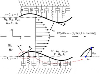
We consider plane pulsatile Poiseuille flow through two compliant walls separated by distance $2L^{\ast }$ , as illustrated by figure 1. We consider as characteristic length scale, $L^{\ast }$ , the half distance of the separation of the compliant walls, as velocity scale the maximum velocity of the steady plane Poiseuille flow, $U_{0}^{\ast }$ , while the forcing angular frequency of the periodic pulsations defines the time scale, $1/\unicode[STIX]{x1D714}_{f}^{\ast }$ (when the forcing frequency tends to zero, a characteristic time scale can be defined through the velocity, $U_{0}^{\ast }$ ). The flow field is then characterized by the Reynolds number, $Re=U_{0}^{\ast }L^{\ast }/\unicode[STIX]{x1D708}_{l}^{\ast }$ , where $\unicode[STIX]{x1D708}_{l}^{\ast }$ is the kinematic viscosity of the fluid, and the Womersley number, $Wo=L^{\ast }(\unicode[STIX]{x1D714}_{f}^{\ast }/\unicode[STIX]{x1D708}_{l}^{\ast })^{1/2}$ , with the Navier–Stokes equations taking the form

(2.1) $$\begin{eqnarray}\displaystyle \frac{Wo^{2}}{Re}\frac{\unicode[STIX]{x2202}\boldsymbol{U}}{\unicode[STIX]{x2202}t}+\boldsymbol{U}\boldsymbol{\cdot }\unicode[STIX]{x1D735}\boldsymbol{U}=-\unicode[STIX]{x1D735}P+\frac{1}{Re}\unicode[STIX]{x1D6FB}^{2}\boldsymbol{U}. & & \displaystyle\end{eqnarray}$$

Figure 1.

Schematic of the system studied.

Here and hereafter, $^{\ast }$ denotes a dimensional quantity. The fluid is assumed to move only in the streamwise direction $x$ due to a mean pressure gradient applied in this direction that changes periodically with a frequency $\unicode[STIX]{x1D714}_{f}^{\ast }$ and amplitude $\unicode[STIX]{x1D6EC}$ ,

(2.2) $$\begin{eqnarray}\displaystyle \frac{\unicode[STIX]{x2202}P_{B}}{\unicode[STIX]{x2202}x}=\frac{\text{d}\overline{P}}{\text{d}x}\left(1+\unicode[STIX]{x1D6EC}\frac{\exp (\text{i}t)+\exp (-\text{i}t)}{2}\right). & & \displaystyle\end{eqnarray}$$

Alternatively, periodic velocity variation with amplitude $\unicode[STIX]{x1D6EC}_{v}$ could be imposed; these relate to the amplitude of the disturbance pressure gradient through $\unicode[STIX]{x1D6EC}_{v}=2\unicode[STIX]{x1D6EC}/Wo^{2}$ . Our choice of $\unicode[STIX]{x1D6EC}$ as the control parameter ensures that finite pumping power is maintained as we vary $Wo$ .

We assume that the mean pressure gradient does not induce vertical displacements of the compliant walls and so in their equilibrium state they rest along $z=\mp 1$ . This assumption extends to the unsteady base flow provided that the vertical wall displacements induced by the fluctuating part of the pressure gradient are small. This is the case for the stiff walls used in the present study, but its effect in yielding a time-varying channel height would need to be incorporated in the calculation of the unsteady base flow when the walls are very flexible. Correspondingly, for the compliant walls that admit axial displacement, we assume that the fluid shear of the base flow is cancelled by the inclusion of pre-tension in the wall.

Decomposing the base velocity field into steady and time-dependent parts, $\boldsymbol{U}_{B}(\boldsymbol{x},t)=\overline{\boldsymbol{U}(\boldsymbol{x})}+\boldsymbol{U}^{\prime }(\boldsymbol{x},t)$ , and taking into account that each part independently satisfies the continuity equation, the fluid momentum equation (2.1), the no-slip boundary conditions on the undeformed compliant walls, we obtain for the steady part,

(2.3a,b ) $$\begin{eqnarray}\displaystyle \overline{U}_{x}=1-z^{2}\quad \text{and}\quad \frac{\text{d}\overline{P}}{\text{d}x}=-\frac{2}{Re}, & & \displaystyle\end{eqnarray}$$

while the time-dependent part of the base flow is given by

(2.4) $$\begin{eqnarray}\displaystyle {U_{x}}^{\prime } & = & \displaystyle q_{-1}\exp (-\text{i}t)+q_{1}\exp (\text{i}t)=\frac{\text{i}\unicode[STIX]{x1D6EC}}{Wo^{2}}\left[1-\frac{\cosh (\text{i}^{3/2}Wo~z)}{\cosh (\text{i}^{3/2}Wo)}\right]\exp (-\text{i}t)\nonumber\\ \displaystyle & & \displaystyle +\frac{\text{i}\unicode[STIX]{x1D6EC}}{Wo^{2}}\left[\frac{\cosh (\text{i}^{1/2}Wo~z)}{\cosh (\text{i}^{1/2}Wo)}-1\right]\exp (\text{i}t),\end{eqnarray}$$

where $z$ is the coordinate normal to the flow direction.

2.2 Perturbation field

2.2.1 Flow field

We proceed by decomposing the velocity field to a base flow field and a field of small-amplitude disturbances which have a spatial exponential form,

(2.5a ) $$\begin{eqnarray}\displaystyle & \displaystyle \boldsymbol{U}(x,y,z,t)=U_{x,B}(z,t)+\unicode[STIX]{x1D716}\boldsymbol{u}(x,y,z,t)=U_{x,B}(z,t)+\unicode[STIX]{x1D716}\hat{\boldsymbol{u}}(z,t)\exp (\text{i}\unicode[STIX]{x1D6FC}x+\text{i}\unicode[STIX]{x1D6FD}y)+\text{c.c.}, & \displaystyle \nonumber\\ \displaystyle & & \displaystyle\end{eqnarray}$$

(2.5b ) $$\begin{eqnarray}\displaystyle & \displaystyle P(x,y,z,t)=P_{B}(x,t)+\unicode[STIX]{x1D716}p(x,y,z,t)=P_{B}(x,t)+\unicode[STIX]{x1D716}\hat{p}(z,t)\exp (\text{i}\unicode[STIX]{x1D6FC}x+\text{i}\unicode[STIX]{x1D6FD}y)+\text{c.c.}, & \displaystyle \nonumber\\ \displaystyle & & \displaystyle\end{eqnarray}$$

where $\unicode[STIX]{x1D716}\ll 1$ , $\unicode[STIX]{x1D6FC},\unicode[STIX]{x1D6FD}$ are the disturbance wavenumbers in the streamwise and spanwise directions, respectively, while the amplitudes of disturbance velocity and pressure, $\hat{\boldsymbol{u}}(z,t)$ , $\hat{p}(z,t)$ depend on time and $\text{c.c.}$ denotes the complex conjugate. Substituting the perturbation forms of (2.5) into the governing equation (2.1) and the continuity equation, and expanding in powers of $\unicode[STIX]{x1D716}$ , we obtain for the $O(\unicode[STIX]{x1D716})$ problem, after subtracting the $O(1)$ problem and eliminating the pressure disturbance,

(2.6) $$\begin{eqnarray}\displaystyle Wo^{2}\frac{\unicode[STIX]{x2202}}{\unicode[STIX]{x2202}t}{\mathcal{L}}\hat{u} _{z}=({\mathcal{L}}-\text{i}\unicode[STIX]{x1D6FC}ReU_{x,B}){\mathcal{L}}\hat{u} _{z}+\text{i}\unicode[STIX]{x1D6FC}Re\frac{\unicode[STIX]{x2202}^{2}U_{x,B}}{\unicode[STIX]{x2202}z^{2}}\hat{u} _{z}, & & \displaystyle\end{eqnarray}$$

where ${\mathcal{L}}=\unicode[STIX]{x2202}^{2}/\unicode[STIX]{x2202}z^{2}-\unicode[STIX]{x1D705}^{2}$ and $\unicode[STIX]{x1D705}^{2}=\unicode[STIX]{x1D6FC}^{2}+\unicode[STIX]{x1D6FD}^{2}$ . Equation (2.6) is recognized as the Orr–Sommerfeld equation for pulsatile flow that supports the well-known flow-based inflectional and Tollmien–Schlichting-wave instabilities and their inter-connectedness that feature in the results that follow.

Using decomposition (2.5), the continuity equation, the streamwise and spanwise part of the Navier–Stokes equations for the $O(\unicode[STIX]{x1D716})$ problem, we can express the pressure disturbance amplitude $\hat{p}(z,t)$ as a function of $\hat{u} _{z}(z,t)$ ,

(2.7) $$\begin{eqnarray}\displaystyle \hat{p}=-\frac{Wo^{2}}{\unicode[STIX]{x1D705}^{2}Re}\frac{\unicode[STIX]{x2202}^{2}\hat{u} _{z}}{\unicode[STIX]{x2202}t\unicode[STIX]{x2202}z}-\frac{\text{i}\unicode[STIX]{x1D6FC}U_{x,B}}{\unicode[STIX]{x1D705}^{2}}\frac{\unicode[STIX]{x2202}\hat{u} _{z}}{\unicode[STIX]{x2202}z}+\frac{\text{i}\unicode[STIX]{x1D6FC}}{\unicode[STIX]{x1D705}^{2}}\frac{\unicode[STIX]{x2202}U_{x,B}}{\unicode[STIX]{x2202}z}\hat{u} _{z}+\frac{1}{\unicode[STIX]{x1D705}^{2}Re}{\mathcal{L}}\frac{\unicode[STIX]{x2202}\hat{u} _{z}}{\unicode[STIX]{x2202}z}. & & \displaystyle\end{eqnarray}$$

2.2.2 Structural model

For the compliant-wall dynamics, we use the two-dimensional isotropic Kirchhoff plate equation with additional terms to account for a dashpot-type damping and a uniformly distributed spring foundation. Combined with the normal force balance on the two compliant walls (Shankar & Kumaran Reference Shankar and Kumaran2002) and keeping only $O(\unicode[STIX]{x1D716})$ terms, we obtain

(2.8) $$\begin{eqnarray}\displaystyle \boldsymbol{n}_{s}\boldsymbol{\cdot }\unicode[STIX]{x1D64F}\boldsymbol{\cdot }\boldsymbol{n}_{s} & = & \displaystyle -p(x,y,z=\mp 1,t)+\frac{2}{Re}\frac{\unicode[STIX]{x2202}u_{z}}{\unicode[STIX]{x2202}z}(x,y,z=\mp 1,t)\mp \frac{2}{Re}\frac{\unicode[STIX]{x2202}U_{x,B}}{\unicode[STIX]{x2202}z}(z=\mp 1,t)\frac{\unicode[STIX]{x2202}\unicode[STIX]{x1D702}_{z,s}}{\unicode[STIX]{x2202}x}\nonumber\\ \displaystyle & = & \displaystyle M_{s}\frac{\unicode[STIX]{x2202}^{2}\unicode[STIX]{x1D702}_{z,s}}{\unicode[STIX]{x2202}t^{2}}+D_{z,s}\frac{\unicode[STIX]{x2202}\unicode[STIX]{x1D702}_{z,s}}{\unicode[STIX]{x2202}t}+K_{s}\unicode[STIX]{x1D702}_{z,s}+B_{s}\left[\frac{\unicode[STIX]{x2202}^{4}\unicode[STIX]{x1D702}_{z,s}}{\unicode[STIX]{x2202}x^{4}}+2\frac{\unicode[STIX]{x2202}^{4}\unicode[STIX]{x1D702}_{z,s}}{\unicode[STIX]{x2202}x^{2}\unicode[STIX]{x2202}y^{2}}+\frac{\unicode[STIX]{x2202}^{4}\unicode[STIX]{x1D702}_{z,s}}{\unicode[STIX]{x2202}y^{4}}\right],\end{eqnarray}$$

where $\boldsymbol{n}_{s}=-(\unicode[STIX]{x2202}\unicode[STIX]{x1D702}_{z,s}/\unicode[STIX]{x2202}x)\boldsymbol{e}_{x}-(\unicode[STIX]{x2202}\unicode[STIX]{x1D702}_{z,s}/\unicode[STIX]{x2202}y)\boldsymbol{e}_{y}\pm \boldsymbol{e}_{z}$ are the linearized unit vectors normal to the two compliant surfaces ( $s=1,2$ lower/upper surfaces) and directed into the fluid domain, $\unicode[STIX]{x1D64F}=-P\unicode[STIX]{x1D644}+(1/Re)[\unicode[STIX]{x1D735}\boldsymbol{U}+(\unicode[STIX]{x1D735}\boldsymbol{U})^{\text{T}}]$ is the total stress tensor of the fluid at the two compliant walls, $\unicode[STIX]{x1D702}_{z,s}(x,y,t)$ , the vertical displacement of the two compliant surfaces, considered positive in the direction of the normal vectors, and $p(x,y,z=\mp 1,t)$ is the non-dimensional pressure disturbance on the compliant walls. The non-dimensional coefficients of compliant-wall inertia, damping, spring-foundation stiffness, flexural rigidity respectively, are defined by

(2.9a-d ) $$\begin{eqnarray}M_{s}=\frac{\unicode[STIX]{x1D70C}_{s}^{\ast }h_{s}^{\ast }\unicode[STIX]{x1D714}_{f}^{\ast 2}L^{\ast }}{\unicode[STIX]{x1D70C}_{l}^{\ast }U_{0}^{\ast 2}},\quad D_{z,s}=\frac{D_{z,s}^{\ast }\unicode[STIX]{x1D714}_{f}^{\ast }L^{\ast }}{\unicode[STIX]{x1D70C}_{l}^{\ast }U_{0}^{\ast 2}},\quad K_{s}=\frac{K_{s}^{\ast }L^{\ast }}{\unicode[STIX]{x1D70C}_{l}^{\ast }U_{0}^{\ast 2}},\quad B_{s}=\frac{B_{s}^{\ast }}{\unicode[STIX]{x1D70C}_{l}^{\ast }U_{0}^{\ast 2}L^{\ast 3}},\end{eqnarray}$$

with $\unicode[STIX]{x1D70C}_{s}^{\ast }$ and $h_{s}^{\ast }$ the material density and thickness, respectively and $B_{s}^{\ast }=E_{s}^{\ast }{h_{s}^{\ast }}^{3}/[12(1-\unicode[STIX]{x1D708}^{2})]$ with $E_{s}^{\ast }$ the elastic modulus and $\unicode[STIX]{x1D708}$ the Poisson ratio (Timoshenko & Woinowsky-Krieger Reference Timoshenko and Woinowsky-Krieger1959), while $\unicode[STIX]{x1D70C}_{l}^{\ast }$ is the fluid density.

2.2.3 Interface conditions

On the compliant surfaces, the perturbation velocity and stresses are each continuous between fluid and solid. Thus, the boundary conditions for the velocity for the $O(\unicode[STIX]{x1D716})$ problem are

(2.10a ) $$\begin{eqnarray}\displaystyle & \displaystyle u_{x}(x,y,z=\mp 1,t)\pm \unicode[STIX]{x1D702}_{z,s}(x,y,t)\frac{\unicode[STIX]{x2202}U_{x,B}}{\unicode[STIX]{x2202}z}(z=\mp 1,t)=0, & \displaystyle\end{eqnarray}$$

(2.10b ) $$\begin{eqnarray}\displaystyle & \displaystyle u_{y}(x,y,z=\mp 1,t)=0, & \displaystyle\end{eqnarray}$$

(2.10c ) $$\begin{eqnarray}\displaystyle & \displaystyle u_{z}(x,y,z=\mp 1,t)=\pm \frac{Wo^{2}}{Re}\frac{\unicode[STIX]{x2202}\unicode[STIX]{x1D702}_{z,s}}{\unicode[STIX]{x2202}t}(x,y,t). & \displaystyle\end{eqnarray}$$

Using the decomposition $\unicode[STIX]{x1D702}_{z,s}(x,y,t)=\hat{\unicode[STIX]{x1D702}}_{z,s}(t)\exp (\text{i}\unicode[STIX]{x1D6FC}x+\text{i}\unicode[STIX]{x1D6FD}y)+\text{c.c.}$ and (2.5) in (2.10) and (2.8), taking into account (2.7) and the continuity equation, we obtain the first boundary condition for the $O(\unicode[STIX]{x1D716})$ problem applied at the compliant surfaces ( $z=\mp 1$ ),

(2.11) $$\begin{eqnarray}\displaystyle & & \displaystyle \pm Wo^{4}\unicode[STIX]{x1D6FC}\frac{\unicode[STIX]{x2202}U_{x,B}}{\unicode[STIX]{x2202}z}\frac{\unicode[STIX]{x2202}^{2}\hat{u} _{z}}{\unicode[STIX]{x2202}t\unicode[STIX]{x2202}z}-\unicode[STIX]{x1D705}^{2}Re^{2}\unicode[STIX]{x1D6FC}\frac{\unicode[STIX]{x2202}U_{x,B}}{\unicode[STIX]{x2202}z}M_{s}\frac{\unicode[STIX]{x2202}\hat{u} _{z}}{\unicode[STIX]{x2202}t}\nonumber\\ \displaystyle & & \displaystyle \qquad =\unicode[STIX]{x1D705}^{2}Re^{2}\unicode[STIX]{x1D6FC}\frac{\unicode[STIX]{x2202}U_{x,B}}{\unicode[STIX]{x2202}z}D_{z,s}\hat{u} _{z}-\text{i}\unicode[STIX]{x1D705}^{2}Wo^{2}Re[B_{s}(\unicode[STIX]{x1D6FC}^{4}+2\unicode[STIX]{x1D6FC}^{2}\unicode[STIX]{x1D6FD}^{2}+\unicode[STIX]{x1D6FD}^{4})+K_{s}]\frac{\unicode[STIX]{x2202}\hat{u} _{z}}{\unicode[STIX]{x2202}z}\nonumber\\ \displaystyle & & \displaystyle \qquad \quad \pm \,\text{i}\unicode[STIX]{x1D6FC}^{2}Wo^{2}Re\frac{\unicode[STIX]{x2202}U_{x,B}}{\unicode[STIX]{x2202}z}\left(\frac{\unicode[STIX]{x2202}U_{x,B}}{\unicode[STIX]{x2202}z}\hat{u} _{z}-U_{x,B}\frac{\unicode[STIX]{x2202}\hat{u} _{z}}{\unicode[STIX]{x2202}z}\right)\nonumber\\ \displaystyle & & \displaystyle \qquad \quad \pm \,Wo^{2}\unicode[STIX]{x1D6FC}\frac{\unicode[STIX]{x2202}U_{x,B}}{\unicode[STIX]{x2202}z}\left(\frac{\unicode[STIX]{x2202}^{3}\hat{u} _{z}}{\unicode[STIX]{x2202}z^{3}}-\unicode[STIX]{x1D705}^{2}\frac{\unicode[STIX]{x2202}\hat{u} _{z}}{\unicode[STIX]{x2202}z}\right),\end{eqnarray}$$

while the enforcement of (2.10c ), taking into account (2.10a ) and the continuity equation, yields the second boundary condition on the compliant surfaces ( $z=\mp 1$ ),

(2.12) $$\begin{eqnarray}\displaystyle \text{i}Wo^{2}\frac{\unicode[STIX]{x2202}U_{x,B}}{\unicode[STIX]{x2202}z}\frac{\unicode[STIX]{x2202}^{2}\hat{u} _{z}}{\unicode[STIX]{x2202}t\unicode[STIX]{x2202}z}=\text{i}Wo^{2}\frac{\unicode[STIX]{x2202}^{2}U_{x,B}}{\unicode[STIX]{x2202}t\unicode[STIX]{x2202}z}\frac{\unicode[STIX]{x2202}\hat{u} _{z}}{\unicode[STIX]{x2202}z}-\unicode[STIX]{x1D6FC}Re\left(\frac{\unicode[STIX]{x2202}U_{x,B}}{\unicode[STIX]{x2202}z}\right)^{2}\hat{u} _{z}. & & \displaystyle\end{eqnarray}$$

2.2.4 Spatial discretization

For spatial discretization in the direction normal to the base flow, $z$ , we use the Chebyshev pseudospectral method. The domain is discretized into $M+1$ collocation points, with their positions given by

(2.13) $$\begin{eqnarray}\displaystyle z(j)=-\cos \left[\frac{(j-1)\unicode[STIX]{x03C0}}{M}\right],\quad \text{for }j=1,M+1, & & \displaystyle\end{eqnarray}$$

and the spatial derivatives of a function at the collocation points are then related to the values of the function there through the Chebyshev differentiation matrices (Canuto et al. Reference Canuto, Hussaini, Quarteroni and Zang1988).

4.1 Floquet analysis through decomposition into a product of exponential growth and sum of harmonics

Following Thomas et al. (Reference Thomas, Bassom, Blennerhassett and Davies2011), the unknown variable $\hat{u} _{z}(z,t)$ is decomposed into a product of exponential growth and a sum of harmonics,

(4.1) $$\begin{eqnarray}\displaystyle \hat{u} _{z}(z,t)=\exp (\unicode[STIX]{x1D707}t)\mathop{\sum }_{n=-N}^{N}\unicode[STIX]{x1D719}_{n}(z)\exp (\text{i}nt), & & \displaystyle\end{eqnarray}$$

where $\unicode[STIX]{x1D707}$ are the Floquet exponents, whose real values define temporal instability(+ve)/stability(-ve) of the system, and $N$ is a large number, typically $N=1000$ , in order to ensure a converged solution. Substituting (4.1) into (2.6) and equating coefficients of harmonics results in

(4.2) $$\begin{eqnarray}\displaystyle \unicode[STIX]{x1D707}Wo^{2}{\mathcal{L}}\unicode[STIX]{x1D719}_{n} & = & \displaystyle -\text{i}\unicode[STIX]{x1D6FC}Re\left(q_{1}{\mathcal{L}}-\frac{\unicode[STIX]{x2202}^{2}q_{1}}{\unicode[STIX]{x2202}z^{2}}\right)\unicode[STIX]{x1D719}_{n-1}\nonumber\\ \displaystyle & & \displaystyle +\,\left({\mathcal{L}}^{2}-\text{i}Wo^{2}n{\mathcal{L}}-\text{i}\unicode[STIX]{x1D6FC}Re\overline{U}_{x,B}{\mathcal{L}}+\text{i}\unicode[STIX]{x1D6FC}Re\frac{\unicode[STIX]{x2202}^{2}\overline{U}_{x,B}}{\unicode[STIX]{x2202}z^{2}}\right)\unicode[STIX]{x1D719}_{n}\nonumber\\ \displaystyle & & \displaystyle -\,\text{i}\unicode[STIX]{x1D6FC}Re\left(q_{-1}{\mathcal{L}}-\frac{\unicode[STIX]{x2202}^{2}q_{-1}}{\unicode[STIX]{x2202}z^{2}}\right)\unicode[STIX]{x1D719}_{n+1}.\end{eqnarray}$$

Relevant expressions for the boundary conditions are obtained by substituting (4.1) into (2.11) and (2.12). The system of equations, comprising (4.2) together with the boundary conditions, is cast as the generalized eigenvalue problem,

(4.3a ) $$\begin{eqnarray}\displaystyle & \displaystyle \unicode[STIX]{x1D63C}\boldsymbol{y}=\unicode[STIX]{x1D707}\unicode[STIX]{x1D63D}\boldsymbol{y}, & \displaystyle\end{eqnarray}$$

(4.3b ) $$\begin{eqnarray}\displaystyle & \displaystyle \boldsymbol{y}=\{\begin{array}{@{}ccccccc@{}}\unicode[STIX]{x1D753}_{-N}^{\text{T}} & \unicode[STIX]{x1D753}_{-N+1}^{\text{T}} & \ldots & \unicode[STIX]{x1D753}_{0}^{\text{T}} & \ldots & \unicode[STIX]{x1D753}_{N-1}^{\text{T}} & \unicode[STIX]{x1D753}_{N}^{\text{T}}\end{array}\}^{\text{T}}, & \displaystyle\end{eqnarray}$$

$\unicode[STIX]{x1D63C}$

$\unicode[STIX]{x1D63D}$

$\unicode[STIX]{x1D753}$

$M+1$

$M=70$

$\unicode[STIX]{x1D707}$

$\boldsymbol{y}$

4.2 Floquet analysis through the monodromy matrix

The system of equations (2.6), with the boundary conditions (2.11) and (2.12) can be written in a similar form to the initial-value problem (3.3),

(4.4a,b ) $$\begin{eqnarray}\displaystyle \frac{\text{d}\hat{\boldsymbol{u}}_{z}}{\text{d}t}=\unicode[STIX]{x1D64C}(t)\hat{\boldsymbol{u}}_{z},\quad \hat{\boldsymbol{u}}_{z}(t=0)=\hat{\boldsymbol{u}}_{z}^{0}, & & \displaystyle\end{eqnarray}$$

where the matrix $\unicode[STIX]{x1D64C}$ is periodic with known period $T$ , due to the imposed periodic base velocity $\boldsymbol{U}_{B}$ . The monodromy matrix $\unicode[STIX]{x1D648}$ is calculated by solving the following initial-value matrix problem (Seydel Reference Seydel1988; Iooss & Joseph Reference Iooss and Joseph1990):

(4.5a,b ) $$\begin{eqnarray}\displaystyle \unicode[STIX]{x1D648}=\unicode[STIX]{x1D64E}(t=T):\quad \frac{\text{d}\unicode[STIX]{x1D64E}}{\text{d}t}=\unicode[STIX]{x1D64C}(t)\unicode[STIX]{x1D64E},\quad \unicode[STIX]{x1D64E}(t=0)=\unicode[STIX]{x1D644}, & & \displaystyle\end{eqnarray}$$

where $\unicode[STIX]{x1D644}$ is the identity matrix, $\unicode[STIX]{x1D64E}(t)=\unicode[STIX]{x1D652}(t)\exp (t\unicode[STIX]{x1D63E})$ , the fundamental matrix, $\unicode[STIX]{x1D652}(t+T)=\unicode[STIX]{x1D652}(t)$ , $T$ -periodic matrix, while the eigenvalues of the monodromy matrix $\unicode[STIX]{x1D648}=\exp (T\unicode[STIX]{x1D63E})=\unicode[STIX]{x1D655}\exp (T\unicode[STIX]{x1D63F})\unicode[STIX]{x1D655}^{-1}$ , called Floquet multipliers $k$ , define the system stability and $\unicode[STIX]{x1D63F}$ the diagonal matrix with components being the Floquet exponents $\unicode[STIX]{x1D707}$ (Schmid Reference Schmid2007); hence $k=\exp (T\unicode[STIX]{x1D707})$ . Finally, the columns of $\unicode[STIX]{x1D655}$ contain the eigenvectors of the matrix $\unicode[STIX]{x1D63E}$ , that correspond to the Floquet exponents. Using a second-order backward-integration scheme for time evolution we obtain at time $n$ ,

(4.6a ) $$\begin{eqnarray}\displaystyle \unicode[STIX]{x1D64E}^{n}=[3\unicode[STIX]{x1D644}-2\unicode[STIX]{x0394}t\unicode[STIX]{x1D64C}^{n}]^{-1}[4\unicode[STIX]{x1D64E}^{n-1}-\unicode[STIX]{x1D64E}^{n-2}], & & \displaystyle\end{eqnarray}$$

(4.6b-d ) $$\begin{eqnarray}\displaystyle \unicode[STIX]{x1D64E}^{0}=\unicode[STIX]{x1D64E}(t=0)=\unicode[STIX]{x1D644},\quad \unicode[STIX]{x1D64E}^{1}=[\unicode[STIX]{x1D644}-\unicode[STIX]{x0394}t\unicode[STIX]{x1D64C}^{1}]^{-1}\unicode[STIX]{x1D64E}^{0},\quad \unicode[STIX]{x1D648}=\unicode[STIX]{x1D64E}(t=T)=\unicode[STIX]{x1D64E}^{N}, & & \displaystyle\end{eqnarray}$$

where we have used for $n=1$ , the first-order backward Euler scheme to initiate the iteration procedure. Alternatively, (4.5) can be integrated explicitly in time using the following iterative algorithm for the solution of the fundamental matrix $\unicode[STIX]{x1D64E}$ (Schmid & Kytomaa Reference Schmid and Kytomaa1994)

(4.7) $$\begin{eqnarray}\displaystyle \unicode[STIX]{x1D64E}_{l+1}^{n}=\unicode[STIX]{x1D644}+\int _{0}^{n}\unicode[STIX]{x1D64C}^{n}\unicode[STIX]{x1D64E}_{l}^{n}\,\text{d}t, & & \displaystyle\end{eqnarray}$$

where the integral of the matrices, calculated with the trapezoidal rule, is taken component-wise and the solution at time $n$ is considered converged after the $(l+1)$ th iteration, when the Frobenius norm of the matrix corresponding to the relative error between consecutive iterations, becomes smaller than a specified value. Following either of the above two numerical procedures for the solution of (4.5), the matrix $\unicode[STIX]{x1D648}$ is evaluated at the end of one period $T$ from the product of the matrices or the sum of the integrals calculated at the previous times, respectively. Its eigenvalues, the Floquet multipliers, $k_{j},j=1,\ldots M+1$ determine the stability of the pulsatile flow through the compliant channel in the following manner: the flow–structure system is stable if $|k_{j}|<1$ for $j=1,2,\ldots M+1$ and unstable if $|k_{j}|>1$ for some $j$ (Iooss & Joseph Reference Iooss and Joseph1990; Tsiglifis & Pelekasis Reference Tsiglifis and Pelekasis2011). In addition, the sign of the real part of the unstable eigenvalue determines how the resulting solution is unstable: if $\text{Im}(k_{j})=0$ with $\text{Re}(k_{j})<-1$ then the unstable solution, $\hat{\boldsymbol{u}}_{z}(t)$ , is periodic with twice the period of that of the base flow, whereas if $\text{Im}(k_{j})=0$ with $\text{Re}(k_{j})>1$ the solution is periodic with the same period of the base flow. Finally, if $\text{Im}(k_{j})\neq 0$ with $|k_{j}|>1$ , the unstable solution is quasi-periodic with characteristic frequencies being those of the base flow and the bifurcating solution, leading to a toroidal structure in the phase space (Iooss & Joseph Reference Iooss and Joseph1990).

4.3 Modal transient growth

The preceding analysis determines whether disturbances amplify in the limit of an infinite number of periods of oscillation. However, during the period, $T$ , of a single pulsation that features inflectional velocity profiles, large modal transient growth of disturbance kinetic energy may occur. This can be advected downstream potentially causing transition to turbulence even though all the Floquet multipliers lie within the unit disk. We are therefore motivated to assess the efficacy of compliant walls in mitigating the total transient energy growth as compared to that generated in a rigid channel. The solution of the systems (4.4) or (3.3) can be written as

(4.8) $$\begin{eqnarray}\displaystyle \hat{\boldsymbol{u}}(t)=\unicode[STIX]{x1D64E}(t)\hat{\boldsymbol{u}}_{z}^{0}. & & \displaystyle\end{eqnarray}$$

Then, the transient growth of the above system at time $t$ maximized over all the initial conditions, quantified by the induced 2-norm of the fundamental matrix $\unicode[STIX]{x1D64E}$ , is:

(4.9) $$\begin{eqnarray}\displaystyle G(t) & = & \displaystyle \max _{\hat{\boldsymbol{u}}_{z}^{0}\neq 0}\frac{\Vert \hat{\boldsymbol{u}}(t)\Vert _{2}^{2}}{\Vert \hat{\boldsymbol{u}}_{z}^{0}\Vert _{2}^{2}}=\max _{\hat{\boldsymbol{u}}_{z}^{0}\neq 0}\frac{\Vert \unicode[STIX]{x1D64E}(t)\hat{\boldsymbol{u}}_{z}^{0}\Vert _{2}^{2}}{\Vert \hat{\boldsymbol{u}}_{z}^{0}\Vert _{2}^{2}}=\Vert \unicode[STIX]{x1D64E}(t)\Vert _{2}^{2}=\unicode[STIX]{x1D70E}_{max}^{2}(\unicode[STIX]{x1D64E}(t))\nonumber\\ \displaystyle & = & \displaystyle \max _{\hat{\boldsymbol{u}}_{z}^{0}\neq 0}\frac{\hat{\boldsymbol{u}}_{z}^{\dagger }(t)\hat{\boldsymbol{u}}_{z}(t)}{\hat{\boldsymbol{u}}_{z}^{\dagger 0}\hat{\boldsymbol{u}}_{z}^{0}}=\max _{\hat{\boldsymbol{u}}_{z}^{0}\neq 0}\frac{\hat{\boldsymbol{u}}_{z}^{\dagger 0}\unicode[STIX]{x1D64E}^{\dagger }(t)\unicode[STIX]{x1D64E}(t)\hat{\boldsymbol{u}}_{z}^{0}}{\hat{\boldsymbol{u}}_{z}^{\dagger 0}\hat{\boldsymbol{u}}_{z}^{0}},\end{eqnarray}$$

where $\unicode[STIX]{x1D70E}_{max}$ is the largest singular value, $\dagger$ is the conjugate transpose and the quotient is recognized as the Rayleigh quotient (Meyer Reference Meyer2000; Schmid & Henningson Reference Schmid and Henningson2001). The maximum total growth, $G(t)$ , at time $t$ , is obtained by finding the largest singular value of the fundamental matrix through singular value decomposition (SVD) or by solving the following eigenproblem for the largest eigenvalue $\unicode[STIX]{x1D706}_{max}$ (Meyer Reference Meyer2000; Schmid & Henningson Reference Schmid and Henningson2001; Mao, Sherwin & Blackburn Reference Mao, Sherwin and Blackburn2009),

(4.10) $$\begin{eqnarray}\displaystyle \unicode[STIX]{x1D64E}^{\dagger }(t)\unicode[STIX]{x1D64E}(t)\hat{\boldsymbol{u}}_{z}^{0}=\unicode[STIX]{x1D706}\hat{\boldsymbol{u}}_{z}^{0}. & & \displaystyle\end{eqnarray}$$

An alternative way to measure the transient growth is by integrating numerically the initial-value problems, (4.4) or (3.3), using a random initial vector $\hat{\boldsymbol{v}}^{0}$ (Von Kerczek Reference Von Kerczek1982) and calculating the time evolution of the total energy of the fluid–structure interaction (FSI), written here for the two-dimensional case and when both vertical and axial displacements of the compliant walls occur as

(4.11) $$\begin{eqnarray}\displaystyle E(t) & = & \displaystyle \frac{1}{2}\int _{-\unicode[STIX]{x03C0}/\unicode[STIX]{x1D6FC}}^{\unicode[STIX]{x03C0}/\unicode[STIX]{x1D6FC}}\hspace{-2.84544pt}\int _{-1}^{1}|u_{x}|^{2}+|u_{z}|^{2}\,\text{d}z\,\text{d}x\nonumber\\ \displaystyle & & \displaystyle +\,\frac{1}{2}\int _{-\unicode[STIX]{x03C0}/\unicode[STIX]{x1D6FC}}^{\unicode[STIX]{x03C0}/\unicode[STIX]{x1D6FC}}M_{s}\left(\frac{\unicode[STIX]{x2202}\unicode[STIX]{x1D702}_{z,s}}{\unicode[STIX]{x2202}t}\right)^{2}+M_{s}\left(\frac{\unicode[STIX]{x2202}\unicode[STIX]{x1D702}_{x,s}}{\unicode[STIX]{x2202}t}\right)^{2}\,\text{d}x\nonumber\\ \displaystyle & & \displaystyle +\,\frac{1}{2}\int _{-\unicode[STIX]{x03C0}/\unicode[STIX]{x1D6FC}}^{\unicode[STIX]{x03C0}/\unicode[STIX]{x1D6FC}}B_{s}\left(\frac{\unicode[STIX]{x2202}^{2}\unicode[STIX]{x1D702}_{z,s}}{\unicode[STIX]{x2202}x^{2}}\right)^{2}+A_{s}\left(\frac{\unicode[STIX]{x2202}\unicode[STIX]{x1D702}_{x,s}}{\unicode[STIX]{x2202}x}\right)^{2}+K_{s}\unicode[STIX]{x1D702}_{z,s}^{2}\,\text{d}x.\end{eqnarray}$$

The first and second integrals respectively correspond to the flow (FKE) and structural kinetic energies (SKE), while the third evaluates the strain energy of the structure (SPE) comprising contributions from plate flexure, plate tension and the spring foundation, respectively, in the order written.

Finally, we remark that details of the calculation of non-modal transient growth are deferred to § 5.3, in which this mechanism is explored in the context of time-asymptotic stability and modal transient growth.

5.1 Steady plane Poiseuille flow

In order to validate the present models, we consider steady Poiseuille flow between two parallel compliant walls with system parameters identical to those given by (4.1) in the two-dimensional analysis of Davies & Carpenter (Reference Davies and Carpenter1997b ), wherein the critical Reynolds number and wavenumber were found, using local spatial stability analysis, to be $Re_{crit.}=6020.5$ and $\unicode[STIX]{x1D6FC}_{crit.}=0.975$ for $\unicode[STIX]{x1D714}_{c}=(Wo^{2}/Re)\unicode[STIX]{x1D714}=0.257$ (see also figure 5 of Davies & Carpenter (Reference Davies and Carpenter1997b )). We therefore use this Reynolds number and streamwise wavenumber, setting $\unicode[STIX]{x1D6FD}=0$ and $\unicode[STIX]{x1D6EC}=0$ in our model with $B_{s}=0.530,K_{s}=2.119$ , $A_{s}=146.9$ and $M_{s}=5.75\times 10^{-6}$ ( $M_{s}^{\prime }=0.333$ when made dimensionless using the characteristic time scale as defined through the centreline velocity) to generate the results presented in figure 2. We remark that for these and subsequent results of the eigen-analysis the variation of velocity perturbations, $u_{z}$ and $u_{x}$ , and the shear stress, $\unicode[STIX]{x1D70F}_{zx}$ , across the channel height are normalized to unity; for clarity the eigenvectors of $u_{x}$ and $\unicode[STIX]{x1D70F}_{zx}$ are plotted over the half-channel height because their variation is anti-symmetric about the channel centreline.

Figure 2.

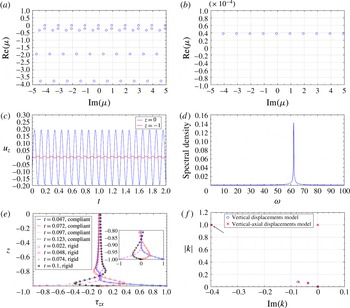
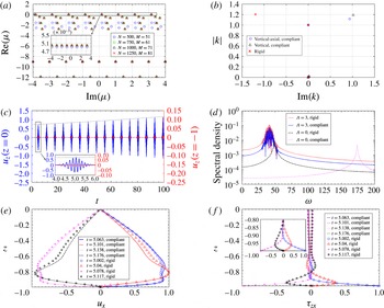
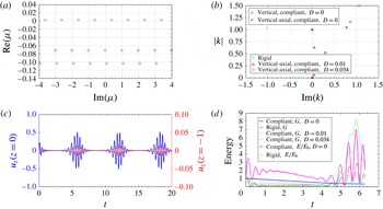
Steady plane Poiseuille flow through a compliant channel at instability onset. (a) Spectrum of the Floquet exponents for the vertical-displacement compliant-wall model. (b) Magnification of (a) to highlight the onset of instability. (c) Time evolution of $u_{z}$ at the channel centreline (blue line) and at the lower compliant wall (red line). (d) Spectral density of the time sequence of $u_{z}$ at the channel centreline. (e) Perturbation shear stress $\unicode[STIX]{x1D70F}_{zx}$ distribution across the channel over one period of oscillations. (f) Spectrum of the Floquet multipliers for the compliant-wall cases. Parameters: $Re_{crit.}=6020.5$ , $\unicode[STIX]{x1D6FC}_{crit.}=0.975$ , $\unicode[STIX]{x1D6FD}=0$ , $Wo=5$ , $\unicode[STIX]{x1D6EC}=0$ with compliant-wall properties the same as those in Davies & Carpenter (Reference Davies and Carpenter1997b ).

Figure 2(a) shows the spectrum of Floquet exponents, with figure 2(b) being a magnification of the region around the least-stable eigenvalues, predicted by the decomposition method for compliant walls with only vertical structural displacements. The onset of instability, evidenced by the marginally positive $\text{Re}(\unicode[STIX]{x1D707})$ , demonstrates that the critical Reynolds number is closely aligned with that found by local spatial stability analysis. It is noted that the Floquet exponents are not unique, in the sense that the $\unicode[STIX]{x1D707}=\text{Re}(\unicode[STIX]{x1D707})+\text{i}[\text{Im}(\unicode[STIX]{x1D707})+m]$ for integer $m$ are also eigenvalues; for this reason, the horizontal distance between the eigenvalues is unity.

Figure 2(c) is a plot of the time dependence of the normal component of the flow disturbance velocity, $u_{z}$ , in the centre of the channel (dashed blue line) and on the lower compliant wall (solid red line). It can be seen that the disturbance velocity oscillates but its amplitude remains constant with time, thereby denoting neutral stability at the chosen (critical) Reynolds number. The oscillation frequency is determined by the spectral density of the time dependence of $u_{z}$ at the channel centre presented in figure 2(d); the value of $\unicode[STIX]{x1D714}=62$ yields $\unicode[STIX]{x1D714}_{c}=0.257$ , which agrees with that of Davies & Carpenter (Reference Davies and Carpenter1997b ) for steady Poiseuille flow. Figure 2(e) shows the eigenvector of disturbance shear stresses $\unicode[STIX]{x1D70F}_{zx}=(1/Re)(\unicode[STIX]{x2202}u_{z}/\unicode[STIX]{x2202}x+\unicode[STIX]{x2202}u_{x}/\unicode[STIX]{x2202}z)$ for the compliant- and rigid-wall cases. Careful comparison reveals that wall compliance serves to increase marginally the concentration of fluid shear stress close to the wall–flow interface, which would then suggest that the compliant wall experiences a slightly higher shear stress than its rigid counterpart.

Finally, figure 2(f) is a plot of the length of the Floquet multipliers against their imaginary part, extracted by the monodromy matrix, considering compliant-wall models with each of vertical and vertical–axial displacements. It can be seen that one system eigenvalue (highlighted by the arrow) has marginally crossed the unit disk, thereby validating the results predicted by the decomposition method. The figure also shows that the inclusion of axial motion in the compliant-wall dynamics has almost no effect on the stability of the fluid–structure interaction for steady Poiseuille flow. It is remarked that the model, which allows both vertical and axial deformations of the compliant walls, has, through the construction of the monodromy matrix, four real Floquet multipliers with length unity, which appear as single point in the figure. These eigenvalues appear as a consequence of analytically taking the time derivative of the two equations (3.2a ) and (3.2b ) at each boundary in order to couch the system in the form (4.5). Alternatively, we can retain the original system in the form

(5.1a,b ) $$\begin{eqnarray}\displaystyle \unicode[STIX]{x1D647}(t)\frac{\text{d}\unicode[STIX]{x1D64E}}{\text{d}t}=\unicode[STIX]{x1D64D}(t)\unicode[STIX]{x1D64E},\quad \unicode[STIX]{x1D64E}(t=0)=\unicode[STIX]{x1D644}, & & \displaystyle\end{eqnarray}$$

and after applying the second-order backward-integration scheme, we obtain the discretized solution equivalent to that of equation (4.6),

(5.2a ) $$\begin{eqnarray}\displaystyle \unicode[STIX]{x1D64E}^{n}=[3\unicode[STIX]{x1D647}^{n}-2\unicode[STIX]{x0394}t\unicode[STIX]{x1D64D}^{n}]^{-1}\unicode[STIX]{x1D647}^{n}[4\unicode[STIX]{x1D64E}^{n-1}-\unicode[STIX]{x1D64E}^{n-2}], & & \displaystyle\end{eqnarray}$$

(5.2b,c ) $$\begin{eqnarray}\displaystyle \unicode[STIX]{x1D64E}^{0}=\unicode[STIX]{x1D64E}(t=0)=\unicode[STIX]{x1D644},\quad \unicode[STIX]{x1D64E}^{1}=[\unicode[STIX]{x1D647}^{1}-\unicode[STIX]{x0394}t\unicode[STIX]{x1D64D}^{1}]^{-1}\unicode[STIX]{x1D647}^{1}\unicode[STIX]{x1D64E}^{0}. & & \displaystyle\end{eqnarray}$$

5.2 Pulsatile plane Poiseuille flow

5.2.1 Modulation frequency $Wo=5$

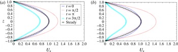
We now focus on the stability of pulsatile Poiseuille flow between compliant walls when $Wo=5$ . This frequency lies within the range of the frequencies encountered in the small vessels of human blood flow. Figures 3(a) and 3(b) show the velocity profiles of the pulsatile base flow for $\unicode[STIX]{x1D6EC}=3$ ( $\unicode[STIX]{x1D6EC}_{v}=2\unicode[STIX]{x1D6EC}/Wo^{2}=0.24$ ) and $\unicode[STIX]{x1D6EC}=5$ ( $\unicode[STIX]{x1D6EC}_{v}=0.4$ ), respectively, during one period of the forcing disturbance pressure gradient. It can be seen that the flow is accelerated during the first half period of the forcing and is decelerated during the second, moving the inflection points away from the wall and towards the centre of the channel.

Figure 3.

Pulsatile velocity profiles during one cycle of the periodic forcing pressure gradient with $Wo=5$ for (a) $\unicode[STIX]{x1D6EC}=3$ ( $\unicode[STIX]{x1D6EC}_{v}=0.24$ ) and (b) $\unicode[STIX]{x1D6EC}=5$ ( $\unicode[STIX]{x1D6EC}_{v}=0.4$ ). Legend in (a) also applies in (b).

Figure 4.

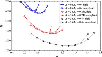
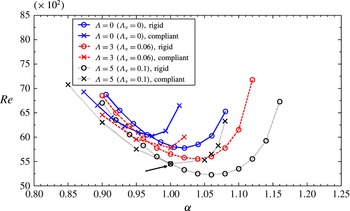
Variation of Reynolds number at which the flow becomes unstable with streamwise wavenumber $\unicode[STIX]{x1D6FC}$ , for rigid and compliant walls and for different values of the modulation amplitude $\unicode[STIX]{x1D6EC}$ . Parameters: $Wo=5$ , $\unicode[STIX]{x1D6FD}=0$ , compliant-wall properties same as defined in (4.1) of Davies & Carpenter (Reference Davies and Carpenter1997b ).

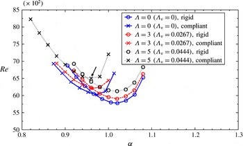
Figure 4 is a plot of the variation of the Reynolds number at which the flow becomes unstable with the streamwise wavenumber for rigid and compliant walls and for different values of the amplitude $\unicode[STIX]{x1D6EC}$ , as predicted by the asymptotic analysis. It is seen that as the amplitude of the pulsation increases, the flow is destabilized significantly relative to the underlying steady Poiseuille flow. This is in agreement with the theoretical work of Von Kerczek (Reference Von Kerczek1982), Singer et al. (Reference Singer, Ferziger and Reed1989), Straatman et al. (Reference Straatman, Khayat, Haj-Qasem and Steinman2002), Thomas et al. (Reference Thomas, Bassom, Blennerhassett and Davies2011) and the experimental observations of Nerem et al. (Reference Nerem, Seed and Wood1972) and Einav & Sokolov (Reference Einav and Sokolov1993), which showed that for low-frequency modulation the flow is always destabilized due to the powerful inviscid (Rayleigh or inflectional) instability. It is also seen that the effect of wall compliance is stabilizing, in that it increases the critical Reynolds number (the minimum for which instability onset occurs), but that this effect diminishes as the amplitude of the flow pulsations is increased.

Figure 5.

(a) Convergence of the Floquet exponents with increasing collocation points ( $N$ ) and Fourier modes ( $M$ ) for the compliant-wall case with vertical displacements. (b) Spectrum of the Floquet multipliers. (c) Time evolution of $u_{z}$ at the channel centreline (blue line) and at the bottom compliant wall (red line); the black dotted line signifies the asymptotic solution, $\exp (\text{Re}(\unicode[STIX]{x1D707})t)$ . (d) Spectral density of the time sequence of $u_{z}$ at the channel centreline. (e) $u_{x}$ and (f) $\unicode[STIX]{x1D70F}_{zx}$ profiles during one cycle of oscillation. Parameters: $Re_{crit.}=3775$ , $\unicode[STIX]{x1D6FC}_{crit.}=1.1$ , $\unicode[STIX]{x1D6FD}=0$ , $Wo=5$ , $\unicode[STIX]{x1D6EC}=3$ , compliant-wall properties same as defined in (4.1) of Davies & Carpenter (Reference Davies and Carpenter1997b ).

Figure 5(a) demonstrates convergence of the most unstable Floquet exponents of the flow over the compliant walls for $\unicode[STIX]{x1D6EC}=3,Re_{crit.}=3775,\unicode[STIX]{x1D6FC}_{crit.}=1.1,\unicode[STIX]{x1D6FD}=0$ (the critical case indicated in figure 4 by a red arrow) with increasing number of collocation points as well as the number of Fourier modes, for the compliant-wall model accounting only for vertical displacements. It can be seen that a converged solution has been obtained for $N=1000$ and $M=71$ . Figure 5(b) shows the corresponding Floquet multipliers for both the rigid and compliant-wall cases for models with and without the axial structural deformations. It can be deduced that the flow within rigid walls is slightly more asymptotically unstable than the flow within compliant walls, and that the inclusion in the model of the axial structural deformations has a small stabilizing effect on the stability of the pulsatile flow through a compliant channel with its walls having the present properties. In addition, since $\text{Im}(k_{j})\neq 0$ with $|k_{j}|>1$ , the unstable modes will have the frequencies both of the base flow and of the bifurcating solution. This can also be observed in figure 5(c), where we show the time evolution of the disturbance velocity $u_{z}$ at the channel centreline and at the lower wall for the compliant-wall case. Figure 5(d) is the spectral density of the channel centreline $u_{z}$ disturbance for $\unicode[STIX]{x1D6EC}=0$ and $\unicode[STIX]{x1D6EC}=3$ , for both the compliant- and rigid-wall cases. It can be seen that the unstable wave-packet contains the fundamental frequency of the base flow but the wave-packet comprises waves with broadband frequencies around the monochromatic frequency of the steady Poiseuille flow between rigid plates at the given Reynolds number.

Figure 6.

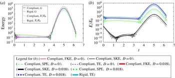
(a) Growth of disturbances during one cycle of modulation, $G$ , and total energy ratio, $E(t)/E(t=0)$ , with time for compliant and rigid walls. (b) Time evolution of the total energy (TE) and its contributions from the flow kinetic energy (FKE), structural kinetic energy (SKE) and structural strain energy (SPE) with and without structural damping $D=D_{x,s}=D_{z,s},s=1,2$ . Parameters: $Re_{crit.}=3775$ , $\unicode[STIX]{x1D6FC}_{crit.}=1.1$ , $\unicode[STIX]{x1D6FD}=0$ , $Wo=5$ , $\unicode[STIX]{x1D6EC}=3$ , compliant-wall properties same as defined in (4.1) of Davies & Carpenter (Reference Davies and Carpenter1997b ).

We remark that for the compliant-wall properties used herein, the lowest in vacuo eigenfrequency for vertical vibrations, $\unicode[STIX]{x1D714}_{vac.}=709.6$ , is far too high to create resonance with the forcing frequency. Therefore, the wall compliance has a very small effect on the distributions of axial-flow, $u_{x}$ , and shear stress, $\unicode[STIX]{x1D70F}_{zx}$ , perturbations across the channel, as can be seen in figure 5(e,f). However, careful scrutiny shows that wall compliance increases the prominence of the single and double maxima that appear through the cycle of the eigenvector of $u_{x}$ , and this effect generates a slightly increased concentration of $\unicode[STIX]{x1D70F}_{zx}$ close to the wall as compared with the rigid-wall case.

Von Kerczek (Reference Von Kerczek1982) showed that disturbances which are predicted to be asymptotically stable at low Womersley number could generate high levels of transient disturbance kinetic energy downstream during the fundamental period $T$ of pulsation due to the inflectional velocity profiles during the deceleration phase of the flow, and this could trigger transition to turbulent flow. In figure 6(a), we show the modal transient growth of disturbances, $G$ , during one cycle of oscillation for flow through rigid- and compliant-walled channels, the latter using the vertical–axial wall-displacement model. This figure also includes the ratio of the total energy of the FSI system, equation (4.11), relative to its initial value, $E(t)/E(t=0)$ , as predicted using the integration of (3.3) for a random initial vector $\hat{\boldsymbol{v}}^{0}$ for both the compliant- and rigid-wall cases. We report that these results correspond to the third period of oscillation in order to discard artificial transient responses from the numerical integration of (3.3) (Von Kerczek Reference Von Kerczek1982). It can be seen that both methods predict similar behaviour, most significantly a five-order increase in the magnitude of the disturbance total energy relative to its initial value and that the effect of wall compliance is mildly mitigating. This large increase of the disturbance total energy during a part of the oscillation cycle for low modulation frequencies is in qualitative agreement with Von Kerczek (Reference Von Kerczek1982) and Singer et al. (Reference Singer, Ferziger and Reed1989), and occurs close to the time $t=3\unicode[STIX]{x03C0}/2$ , when there is the maximum flow deceleration and the inflection points of the velocity profile are far from the walls.

In order to reveal how the total energy (TE) during modal transient growth is distributed during the oscillation cycle and demonstrate the effect of structural damping on it, we plot in figure 6(b) the time evolution of the system TE and its components, namely, the flow kinetic energy (FKE), the structural kinetic energy (SKE) and the structural strain energy (SPE) for zero and at large values (that of critical damping $D_{crit.}=2\sqrt{M_{s}K_{s}}$ ) of the structural damping as well as the case of flow in a rigid-walled channel. It can be seen that most of the TE of the system comprises kinetic energy of the flow, with a small contribution from the strain energy of the wall and negligible contribution from the structural kinetic energy. This reflects the fact that, for the dynamics of the compliant wall given by its properties alongside the chosen modulation frequency, the wall compliance exercises negligible stabilizing effect, as also seen in the results of the asymptotic analysis in figure 4 for $\unicode[STIX]{x1D6EC}=3$ . In addition, the inclusion of a large level of structural damping $D=D_{x,s}=D_{z,s},s=1,2$ has a small destabilizing effect on the transient response, which manifests itself by an almost one order of magnitude larger maximum flow kinetic energy than that found for the flow through a compliant channel without damping.

Figure 7.

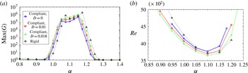
(a) Maximum total amplification of the disturbances, at $Re_{crit.}=3775$ . (b) Reynolds number at which the flow becomes unstable versus the streamwise wavenumber, $\unicode[STIX]{x1D6FC}$ , for different values of structural damping $D=D_{x,s}=D_{z,s},s=1,2$ . Parameters: $Wo=5,\unicode[STIX]{x1D6EC}=3,\unicode[STIX]{x1D6FD}=0$ , compliant-wall properties same as defined in (4.1) of Davies & Carpenter (Reference Davies and Carpenter1997b ). Legend in (a) also applies in (b).

Cooper & Carpenter (Reference Cooper and Carpenter1997) studied the stability of rotating-disc boundary-layer flow over a compliant wall and found that structural damping has a destabilizing effect on the inviscid (Type I) inflectional instability, and therefore this is categorized as a Class A instability in the energy classification scheme of Benjamin (Reference Benjamin1960, Reference Benjamin1963) and Landahl (Reference Landahl1962). Figures 7(a) and 7(b) respectively show the maximum disturbance growth, $G$ , during the fundamental period of the forcing cycle at $Re_{crit.}=3775$ (the rigid-wall value for $Wo=5$ and $\unicode[STIX]{x1D6EC}=3$ ) and the Reynolds number of instability onset as functions of the streamwise wavenumber of the disturbances. We remark that two peaks are resolved in figure 7(a), and conjecture that the distinct wavenumbers at which these occur relate to the positive and negative base-flow fluctuations superimposed upon the positive mean flow within the pulsation cycle. The results arising from different levels of structural damping, $D=D_{x,s}=D_{z,s},s=1,2$ , up to its critical value are included in figure 7(a,b). It can be seen that structural damping destabilizes both the transient and the time-asymptotic responses of the FSI system, with a more pronounced effect on the latter. In addition, for the highest value of structural damping, the FSI system exhibits approximately a half order of magnitude larger maximum total growth than that of the corresponding flow through a rigid channel, which is similar to findings of figure 6(b). We also note here that the shear-stress distribution (result not shown) is almost identical to that of the corresponding undamped compliant-wall case of figure 5(f), with structural damping generating a marginal increase in the concentration of shear stress close to the wall.

Before closing this section, we briefly relate the present findings to human blood flow. Although the properties of the compliant walls used herein and the resulting critical Reynolds numbers are dissimilar from those in the carotid artery, the present results suggest that an increase in the stiffness and/or the damping of the arterial walls might change the characteristics of the flow within the forcing cycle by causing transition from laminar to turbulent flow, and thus creating the conditions for the establishment of atherosclerotic plaque. In such flows the maintenance of laminar-flow shear stress is crucial for normal vascular function and the inhibition of proliferation, thrombosis and inflammation of the vessel wall (Cunningham & Gotlieb Reference Cunningham and Gotlieb2005). This echoes the clinical research of Armentano et al. (Reference Armentano, Barra, Santana, Pessana, Graf, Craiem, Brandani, Baglivo and Sanchez2006), who found that the arterial walls of people suffering from arterial hypertension are characterized by a lower compliance and a larger wall-material viscosity. Furthermore, Alexander (Reference Alexander1995) reported that hypertension, which correlates with vessel stiffening, increases the risk of atherosclerosis.

5.2.2 Modulation frequency $Wo=10$

We now focus on the case with frequency modulation of the base flow at $Wo=10$ using the same compliant-wall properties as when $Wo=5$ above. Figure 8 shows the variation of the Reynolds number at instability onset with streamwise wavenumber, $\unicode[STIX]{x1D6FC}$ , for both rigid and compliant channel walls and different values of modulation amplitude, $\unicode[STIX]{x1D6EC}$ . The flow is destabilized by increasing $\unicode[STIX]{x1D6EC}$ , but to a lesser extent than that seen for $Wo=5$ in figure 4. Wall compliance is again seen to have a stabilizing effect at for each $\unicode[STIX]{x1D6EC}$ -case, and this effect is greater than that seen in the corresponding results at $Wo=5$ . This is because the higher modulation frequency is better matched to the natural frequency of the compliant-wall structural dynamics.

Figure 8.

Variation of the Reynolds number at instability onset with the streamwise wavenumber $\unicode[STIX]{x1D6FC}$ , for rigid and compliant walls for different values of the modulation amplitude $\unicode[STIX]{x1D6EC}$ . Parameters: $Wo=10$ , $\unicode[STIX]{x1D6FD}=0$ , compliant-wall properties same as defined in (4.1) of Davies & Carpenter (Reference Davies and Carpenter1997b ).

Figure 9.

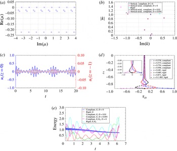
(a) Spectrum of the Floquet exponents for the compliant-wall case. (b) Spectrum of the Floquet multipliers for vertical and axial–vertical compliant-wall models and with different levels of structural damping. (c) Time evolution of $u_{z}$ at the centreline of the channel (blue line) and at the bottom compliant wall (red line). (d) Growth of disturbances, $G$ , and total energy ratio, $E(t)/E(t=0)$ , with time for compliant and rigid walls and for different values of the structural damping. Parameters: $Re_{crit.}=5475$ , $\unicode[STIX]{x1D6FC}_{crit.}=1.0$ , $\unicode[STIX]{x1D6FD}=0,Wo=10$ , $\unicode[STIX]{x1D6EC}=5$ , compliant-wall properties same as defined in (4.1) of Davies & Carpenter (Reference Davies and Carpenter1997b ).

Figure 9(a) shows the most unstable Floquet exponents of the flow over the compliant wall for the model with vertical displacements for $\unicode[STIX]{x1D6EC}=5,Re_{crit.}=5475,\unicode[STIX]{x1D6FC}_{crit.}=1.0,\unicode[STIX]{x1D6FD}=0$ (the case indicated in figure 8 with the black arrow). Figure 9(b) is a plot of the corresponding Floquet multipliers predicted by the time-stepping technique (monodromy matrix) for each of the vertical and axial–vertical displacement compliant-wall models and for different levels of structural damping (the maximum being critical damping). As in the $Wo=5$ case, structural damping has a destabilizing effect on the inflectional instability mechanism. Since $\text{Im}(k_{j})\neq 0$ with $|k_{j}|>1$ , the unstable solution will have frequencies both of the base flow and of the unstable solution. This can also be observed in figure 9(c), where we show the time evolution of the disturbance velocity $u_{z}$ at the channel centreline and on the bottom wall for the compliant-wall case. It can be seen that the relative size of the wall disturbance velocity contribution is larger than of the corresponding $Wo=5$ case (figure 5 c); this again indicates increased fluid–structure interaction between the flow modulation and structural frequencies at this higher $Wo$ .

In figure 9(d) we show the growth of the disturbances, $G$ , over one cycle of the pressure modulation for flow through rigid and compliant channels as well as the time evolution of the total energy ratio, $E(t)/E(t=0)$ , predicted by the numerical integration with random initial conditions, for the conditions at the point marked with the black arrow in figure 8 and for different levels of structural damping. As in the $Wo=5$ case, structural damping increases mildly the maximum modal transient growth, $G$ , as compared with flow through a rigid channel. However, this result (and that in figure 11(e) for $\unicode[STIX]{x1D6FD}=0$ that is presented later), suggests that up to a pressure-modulation amplitude of $\unicode[STIX]{x1D6EC}=5$ , transient effects are relatively small for $Wo\geqslant 10$ and that the asymptotic analysis should be adequate for the practical prediction of the system’s stability with respect to the energy growth of disturbances.

5.2.3 Modulation frequency $Wo=15$

We proceed by further increasing the frequency modulation to $Wo=15$ , keeping the compliant-wall properties unchanged. Figure 10 shows that the flow is now stabilized by the modulation, in contrast to the effect at the lower values of $Wo$ studied in the previous subsections. This is in agreement with the work of Thomas et al. (Reference Thomas, Bassom, Blennerhassett and Davies2011), in which it was found that modulation stabilizes plane oscillatory Poiseuille flow for $Wo\geqslant 10\sqrt{2}$ . As found for the lower $Wo$ cases, wall compliance continues to be stabilizing, but its effect is increased when a higher amplitude modulation is applied.

Figure 10.

Variation of the Reynolds number at which the flow becomes unstable with the streamwise wavenumber $\unicode[STIX]{x1D6FC}$ , for rigid and compliant walls and for different values of the modulation amplitude $\unicode[STIX]{x1D6EC}$ . Parameters: $Wo=15$ , $\unicode[STIX]{x1D6FD}=0$ , compliant-wall properties same as defined in (4.1) of Davies & Carpenter (Reference Davies and Carpenter1997b ).

Figure 11.

(a) Spectrum of the Floquet exponents for the compliant-wall case. (b) Spectrum of the Floquet multipliers for vertical and axial–vertical compliant-wall models and with different levels of structural damping. (c) Time evolution of $u_{z}$ at the centreline of the channel (blue line) and at the bottom compliant wall (red line). (d) $\unicode[STIX]{x1D70F}_{zx}$ distribution over one period of oscillation. (e) Growth of disturbances, $G$ , and total energy ratio, $E(t)/E(t=0)$ , with time for compliant and rigid walls and for different values of the structural damping. Parameters: $Re_{crit.}=6500$ , $\unicode[STIX]{x1D6FC}_{crit.}=0.96$ , $\unicode[STIX]{x1D6FD}=0$ , $Wo=15$ , $\unicode[STIX]{x1D6EC}=5$ , compliant-wall properties same as defined in (4.1) of Davies & Carpenter (Reference Davies and Carpenter1997b ).

Figure 11(a) shows the most unstable Floquet exponents of the flow through the channel with the vertical-displacement compliant-wall model for $\unicode[STIX]{x1D6EC}=5$ , $Re_{crit.}=6500$ , $\unicode[STIX]{x1D6FC}_{crit.}=0.96$ and $\unicode[STIX]{x1D6FD}=0$ , and without structural damping (the critical case indicated with the black arrow in figure 10). Figure 11(b) plots the corresponding Floquet multipliers predicted by the eigenvalues of the monodromy matrix for the vertical and vertical–axial structural displacements models for different levels of the structural damping (the maximum being critical damping); clearly, structural damping destabilizes the time-asymptotic behaviour of the FSI system. The compliant-wall displacement velocities are larger relative to the previous cases at lower $Wo$ but, as seen in figure 11(d), wall compliance continues to cause only a marginal increase in the shear-stress concentration close to the wall. Finally, in figure 11(e) we show the transient growth of disturbances, $G$ , and the total energy ratio, $E(t)/E(t=0)$ , during one cycle of the pressure modulation for different values of the structural damping, where it can be seen that the modal transient growth of the total energy of disturbances is negligible in all cases.

Figure 12.

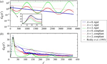
Energy growth of disturbances $G_{E}(t^{\prime })$ with time $t^{\prime }$ for different values of the modulation amplitude $\unicode[STIX]{x1D6EC}$ for rigid and compliant walls. (a) $Wo=5$ and (b) $Wo=15$ . The dotted and dashed-dotted lines represent the asymptotic solution of the least-stable Floquet exponents, $\exp (2\text{Re}(\unicode[STIX]{x1D707})t)$ , for the rigid and compliant walls, respectively. Parameters: $Re=5000$ , $\unicode[STIX]{x1D6FC}=1$ , $\unicode[STIX]{x1D6FD}=0$ , compliant-wall properties same as defined in (4.1) of Davies & Carpenter (Reference Davies and Carpenter1997b ).

5.3 Non-modal transient growth

It should be stressed that the previous results concern modal asymptotic analysis and modal transient growth that occurs within the fundamental cycle of pulsation. However, it has been proposed by Schmid (Reference Schmid2007) that non-modal stability theory could explain the discrepancy between the predictions of modal analysis and experimental results at pulsatile-flow frequencies relevant to blood flow in arteries. Disturbances that are predicted to be stable in the Floquet analysis could induce high levels of non-modal transient disturbance kinetic energy downstream during the fundamental period $T$ of pulsation, or from period to period, due to the non-orthogonality of the eigenmodes of the Navier–Stokes operator. In order to assess the potential of disturbances to generate significant levels of total energy through a non-modal mechanism, and compare these with those produced by modal transient growth, we define the transient growth $G_{E}$ , quantified by the energy norm of the fundamental matrix $\unicode[STIX]{x1D64E}$ , as

(5.3) $$\begin{eqnarray}\displaystyle G_{E}(t)=\max _{\hat{\boldsymbol{u}}_{z}^{0}\neq 0}\frac{\Vert \hat{\boldsymbol{u}}(t)\Vert _{E}^{2}}{\Vert \hat{\boldsymbol{u}}_{z}^{0}\Vert _{E}^{2}}=\max _{\hat{\boldsymbol{u}}_{z}^{0}\neq 0}\frac{\Vert \unicode[STIX]{x1D641}(t)\exp (\unicode[STIX]{x1D646}t)\hat{\boldsymbol{u}}_{z}^{0}\Vert _{2}^{2}}{\Vert \unicode[STIX]{x1D641}(t)\hat{\boldsymbol{u}}_{z}^{0}\Vert _{2}^{2}}=\Vert \unicode[STIX]{x1D641}(t)\exp (\unicode[STIX]{x1D646}t)\unicode[STIX]{x1D641}^{-1}(t)\Vert _{2}^{2}, & & \displaystyle\end{eqnarray}$$

where $\unicode[STIX]{x1D642}=\unicode[STIX]{x1D641}^{\text{T}}\unicode[STIX]{x1D641}$ is the Gramian matrix corresponding to the total energy equation (4.11), assembled using the eigenvectors of the fundamental matrix $\unicode[STIX]{x1D64E}$ and $\unicode[STIX]{x1D646}$ , the diagonal matrix with components being its eigenvalues at each time step. In figure 12(a,b) we plot the transient energy growth $G_{E}$ versus the time $t^{\prime }$ (with characteristic time defined through the centreline velocity, i.e. $t^{\prime }=tU_{0}^{\ast }/(\unicode[STIX]{x1D714}_{f}^{\ast }L^{\ast })$ ) for different modulation amplitudes, $\unicode[STIX]{x1D6EC}$ , for rigid and compliant walls when $Re=5000$ and $\unicode[STIX]{x1D6FC}=1$ at each of low ( $Wo=5$ ) and high ( $Wo=15$ ) modulation frequencies.

Considering first the rigid-wall results in figure 12(a), it is seen that at $Wo=5$ the energy growth due to modal effects in pulsatile flow vastly exceeds that due to non-modal effects, as can be discerned by comparing the values of the inset figure, which highlights the non-modal growth and uses a linear vertical scale, with those of the main figure 12(a). Of course, when the base flow is steady ( $\unicode[STIX]{x1D6EC}=0$ ) only non-modal transient growth occurs; for this case excellent agreement is seen between the result of our calculation and that of Reddy et al. (Reference Reddy, Schmid and Henningson1993). In contrast, figure 12(b) shows that at high-frequency modulation, $Wo=15$ , the non-modal energy-growth mechanism is stronger than that of the modal mechanism. However, at this frequency the levels of total energy extracted from the mean flow are orders of magnitude smaller those that occur for low-frequency modulation due to modal effects, as seen in figure 12(a), where a logarithmic scale has been used for the vertical axis. Again, we show excellent agreement between our results and those of Reddy et al. (Reference Reddy, Schmid and Henningson1993). For both low- and high-frequency cases it is noted that as the modulation amplitude is increased, non-modal transient growth decreases slightly while modal transient growth increases significantly; for the low-frequency case it is seen that $\unicode[STIX]{x1D6EC}=2$ is sufficiently high that the flow is also asymptotically unstable. In addition, it can be observed from the dashed lines that the energy variation from period to period arising from modal effects closely follows the growth/decay predicted by the least-stable Floquet exponents, $\exp (2\text{Re}(\unicode[STIX]{x1D707})t)$ , from the asymptotic analysis.

We now discuss the modelling and effect of wall compliance in the transient results presented in figure 12. Hœpffner et al. (Reference Hœpffner, Bottaro and Favier2010) showed that wall compliance in steady plane Poiseuille flow increased (relative to rigid walls) the energy growth due non-modal transient growth. They obtained converged results by projecting onto the 30 least-stable eigenmodes; instability associated with the presence of spurious modes took place if this number of modes was increased excessively. This appears to be a common problem in systems, such as the present, where interfaces exist. It can be ameliorated if the order of the derivatives in the Orr–Sommerfield and the dynamic interfacial equations are reduced (Malik & Hooper Reference Malik and Hooper2007). Accordingly, we solved for the primitive variables $u_{x}$ and $u_{z}$ explicitly, and thus reduced the order of the highest derivative by one for the field and dynamic interfacial equations (2.6) and (2.8). By doing so, convergence was achieved by projecting onto the 40 least-stable eigenmodes; however, a small-amplitude short-wavelength instability still persists, especially in the later stages of the modal growth; this is most prominent for high-frequency modulation. Figure 12(a,b) shows that wall compliance increases the non-modal energy growth, in that the maximum of energy increases, but reduces the modal transient growth for both low- and high-frequency modulation. However, due to the high value of wall stiffness used herein, the effects are fairly small. This is in qualitative agreement with the results of Hœpffner et al. (Reference Hœpffner, Bottaro and Favier2010), who showed that by increasing the wall stiffness the non-modal energy growth tended to that of the rigid-wall system for steady plane Poiseuille flow. Finally, as seen for rigid walls, figure 12(a,b) show good agreement between modal growth/decay from period to period with that predicted by the least-stable Floquet exponents.

As can be seen from figure 12(a,b), the non-modal energy growth may be significant in the early stages of evolution of the initial perturbation, while at later times it is the modal energy growth and asymptotic stability that govern the system dynamics. This is especially the case for low-frequency modulation. For high-frequency modulation the combined effects of non-modal and modal transient growth are seen to be small. We also remark that for high-frequency modulation the non-modal results for pulsatile flow should be treated with caution because the modelling effectively assumes that the time scales on which the non-orthogonal stable eigenmodes decay must be vanishingly small compared with the period of pulsation; this is exactly true for steady flow, closely adhered to for a low-frequency unsteady base flow as seen in figure 12(a), but is seen not to be the case for high-frequency modulation in figure 12(b). Overall, since the contribution of non-modal transient growth is small relative to that of modal transient growth, we will focus on the latter for the remainder of this paper. However, it is acknowledged that non-modal transient growth can play a significant rôle for three-dimensional disturbances and/or for more flexible compliant walls (Hœpffner et al. Reference Hœpffner, Bottaro and Favier2010). For example, Schmid (Reference Schmid2007) predict that the maximum transient energy growth of oblique disturbances in rigid-walled channel flow can be up to $O(10^{4})$ .

Figure 13.

Critical Reynolds number versus $Wo$ , for rigid and compliant walls and for different values of the amplitude $\unicode[STIX]{x1D6EC}$ and $\unicode[STIX]{x1D6FD}=0$ . Compliant-wall properties same as those defined in (4.1) of Davies & Carpenter (Reference Davies and Carpenter1997b ).

5.4 Summary of modulation-frequency effects in plane Poiseuille flow

We now focus on the onset of instability, and therefore figure 13 summarizes the variation of critical Reynolds number with the modulation frequency, $Wo$ . It can be seen that for a given modulation amplitude there exists a range of $Wo$ (approximately for $Wo=10$ –30) where compliant-wall effects significantly stabilize the flow, as evidenced by higher critical Reynolds numbers than those of the corresponding rigid channel result. Beyond this range, compliance continues to have a marginally stabilizing effect. It is also noted that for both rigid and compliant channels the effect of modulation is stabilizing for $Wo\gtrapprox 13$ , while below this value it is strongly destabilizing as compared with the stability of steady plane Poiseuille flow ( $\unicode[STIX]{x1D6EC}=0$ results in the figure).

The present results indicate that as $Wo\rightarrow \infty$ both the rigid and compliant channel results asymptotically approach their corresponding steady base-flow critical Reynolds numbers. This might appear counter-intuitive, and contradicts the findings of Von Kerczek (Reference Von Kerczek1982) and Singer et al. (Reference Singer, Ferziger and Reed1989), who showed stabilization when the modulation frequency is close to that of the frequency of neutrally stable disturbances in steady Poiseuille flow ( $Wo=98.85$ ). However, in the present work we have applied the modulation via a pressure forcing that has a defined amplitude. This means that as $Wo$ is increased then the amplitude of the base-flow velocity variation is reduced; in the limit $Wo\rightarrow \infty$ , the base-flow velocity variation is zero and the base flow is therefore steady. To illustrate this point of difference, Von Kerczek (Reference Von Kerczek1982) and Singer et al. (Reference Singer, Ferziger and Reed1989) used a velocity-modulation amplitude $\unicode[STIX]{x1D6EC}_{v}=0.105$ at $Wo=98.85$ , whereas our application of a pressure-modulation amplitude $\unicode[STIX]{x1D6EC}=5$ leads to $\unicode[STIX]{x1D6EC}_{v}=2\unicode[STIX]{x1D6EC}/Wo^{2}=0.001$ . In most physical systems it is the imposition of a pressure modulation with finite magnitude that would generate the unsteady base flow, while the assumption of a fixed velocity modulation at very high frequencies would lead to unfeasible power requirements of the pumping system. The fact that, in the present study, the critical Reynolds numbers for both rigid and compliant channels approach those of steady Poiseuille flow provides further evidence that the inflectional instability which dominates the system behaviour at low to intermediate $Wo$ -values is of Class A. This is because its neutral-stability branch becomes that of the TSW branch at high $Wo$ – that continues to exist for steady base flow – and it is well known that TSWs are Class A instabilities.

Figure 13 also suggests that there is an additive effect from the combination of Stokes-layer and the compliant-wall stabilization. For a given amplitude of the pressure modulation, the thickness of the Stokes layer $\unicode[STIX]{x1D6FF}=(2\unicode[STIX]{x1D708}_{l}^{\ast }/\unicode[STIX]{x1D714}_{f}^{\ast })^{1/2}$ reduces as the modulation frequency increases and the stabilizing effects of the Stokes layer decrease; this trend is replicated for the corresponding compliant-wall cases, albeit at higher critical Reynolds numbers, indicating that the action of the compliant walls does not modify Stokes-layer effects in pulsatile plane Poiseuille flow. Finally, we report that the critical streamwise number that yields the critical Reynolds number is decreased by wall compliance, a feature seen in figures 4, 8 and 10, while for all cases decreasing $Wo$ leads to higher values of critical wavenumber.

5.5 Three-dimensional disturbances in pulsatile plane Poiseuille flow

All of the foregoing analyses have been restricted to two-dimensional disturbances, hence $\unicode[STIX]{x1D6FD}=0$ . We now investigate the effect of oblique waves on the stability of plane pulsatile flow over compliant walls. For the relatively stiff compliant walls used in the present work, figure 14(a) shows that three-dimensional waves are asymptotically more stable than their two-dimensional counterparts over the entire range of modulation frequencies, $Wo$ , examined for both steady and pulsatile flow with pressure modulation $\unicode[STIX]{x1D6EC}=3$ because their corresponding critical Reynolds numbers are higher. It is also seen in figure 14(a) that wall compliance is more effective in the stabilization of oblique waves than for their two-dimensional counterparts. Figure 14(b) shows the variation of the streamwise wavenumber that yields the critical Reynolds number. The variations with $Wo$ seen for each value of transverse wavenumber, $\unicode[STIX]{x1D6FD}$ , for each modulation amplitude are similar to those identified in § 5.3, as is the difference between rigid- and complaint-wall systems. Overall, increasing $\unicode[STIX]{x1D6FD}$ decreases the critical wavenumber. However, there is one striking departure for the compliant-wall case with $\unicode[STIX]{x1D6EC}=3$ and $\unicode[STIX]{x1D6FD}=1$ , where a jump in critical wavenumber occurs between $Wo=8$ and 10. This corresponds to a switch of modes and is discussed below.

Figure 14.

Variation of (a) critical Reynolds number and (b) critical wavenumber with $Wo$ , for rigid and compliant walls for different values of the spanwise wavenumber, $\unicode[STIX]{x1D6FD}$ . Compliant-wall properties same as those defined in (4.1) of Davies & Carpenter (Reference Davies and Carpenter1997b ).

Throughout this paper we have used compliant-wall properties that have been sufficiently stiff that travelling-wave flutter (TWF) has not been the critical mode for destabilization. However, for the high Reynolds numbers associated with system destabilization at $\unicode[STIX]{x1D6EC}=3$ and $\unicode[STIX]{x1D6FD}=1$ , TWF replaces the inflectional instability as the critical mode when $Wo>10$ . This wall-based instability has much higher wavenumber, as can be seen in figure 14(b). Close inspection of the critical Reynolds-number variation at $\unicode[STIX]{x1D6EC}=3$ , $\unicode[STIX]{x1D6FD}=1$ in figure 14(a) reveals that this instability branch remains below the value of the critical Reynolds number for the corresponding steady base-flow result for all $Wo>10$ , and significantly lower than the critical Reynolds number for the rigid-walled channel (in which TWF cannot exist). For the TWF instability, there is no range of $Wo$ for which base-flow pulsation is stabilizing, and this therefore suggests that the Stokes layer is a further destabilizing source of irreversible energy transfer from the flow to the wall.

TWF is a Class B instability and for this reason is stabilized by structural damping. This is seen in figure 15(a), which shows the variation of Reynolds number at instability onset with streamwise wavenumber with different amounts of structural damping for the case with $Wo=15$ , $\unicode[STIX]{x1D6EC}=3$ and $\unicode[STIX]{x1D6FD}=1$ . Clearly there exist two types of instability branches: the rigid and compliant channel branch at lower wavenumbers associated with inflectional instability, while the second, at higher wavenumbers, for the compliant channel is that of TWF. For an elastic wall, the TWF branch yields a critical Reynolds number lower than that of the rigid-walled system, and this continues to hold for an incremental level of damping that is seen to be stabilizing. However, when a sufficiently high level of structural damping is present, the critical Reynolds number of TWF exceeds that of the inflectional instability of the pulsatile flow through a rigid channel. At the same time, the structural damping destabilizes the inflectional instability branch of the compliant channel, and it may become the critical instability.

Figure 15.

(a) Variation of Reynolds number at which the flow becomes unstable with the streamwise wavenumber for different levels of structural damping for the compliant-wall case when $Wo=15$ , $\unicode[STIX]{x1D6EC}=3$ and $\unicode[STIX]{x1D6FD}=1$ . II and TWF denote Inflectional and TWF instability branches, respectively. (b) Maximum amplification of disturbances for the case with $Wo=5,\unicode[STIX]{x1D6EC}=3,Re_{crit.}=3775$ against the streamwise wavenumber, $\unicode[STIX]{x1D6FC}$ , for different transverse wavenumbers, $\unicode[STIX]{x1D6FD}$ . Compliant-wall properties same as those defined in (4.1) of Davies & Carpenter (Reference Davies and Carpenter1997b ).

While the structure of neutral-stability curves in figure 15(a) parallels that found in Davies & Carpenter (Reference Davies and Carpenter1997a ) for steady flow through a compliant channel using a two-dimensional analysis ( $\unicode[STIX]{x1D6FD}=0$ ) wherein TSWs and TWF are the principal system instabilities, the static divergence instability that they also found at low wavenumbers is absent in our results. We remark that for their figure 7, Davies & Carpenter (Reference Davies and Carpenter1997a ) used a tensioned membrane instead of a spring-backed plate, and this resulted in a very flexible channel that is more prone to wall-based instabilities. For the spring-backed flexible plate used in our system, an equivalent critical Reynolds number predicted for the onset of two-dimensional divergence instability for steady inviscid fluid flow in a compliant channel (Burke et al. Reference Burke, Lucey, Howell and Elliott2014) is $Re_{D}\approx 1.25\times 10^{4}$ , having chosen blood for the fluid and a characteristic dimension typical of a small blood vessel. This value falls within the range of Reynolds numbers in figure 15(a). However, potential flow is known to yield a very low estimate of divergence-onset flow speed (equivalent Reynolds number) because it does not account for the effects of flow shear (Davies Reference Davies2003; Kapor & Lucey Reference Kapor, Lucey, Meskell and Bennet2012). In addition, it has been shown by Lucey & Carpenter (Reference Lucey and Carpenter1993) that two-dimensional disturbances give significantly lower values of divergence-onset flow speed than their three-dimensional counterparts. The combination of these effects accounts for the fact that we do not find divergence eigenmodes in the range of Reynolds numbers used to generate figure 15(a).

In closing this subsection, we emphasize that for the present parameters, the stability of the system will be determined by the inflectional instability of plane waves with $\unicode[STIX]{x1D6FD}=0$ . Nevertheless, for compliant channels with more flexible walls than those used in the present paper, the existence of TWF or divergence may determine the stability bounds for certain combinations of system parameters. Finally, a transient modal analysis yielding the results presented in figure 15(b) predicts that the maximum amplification of the total energy of system disturbances, $G$ , reduces as the wavelength of the spanwise disturbances decreases for both rigid and compliant channels.