1 Introduction
The wake of a fluid passing a solid obstacle exhibits different behaviours depending on the associated Reynolds number. A generally stable regime with a laminar two-dimensional von Kármán vortex shedding is observed at low Reynolds numbers between 49 and 150 (Davis, Moore & Purtell Reference Davis, Moore and Purtell1984; Williamson Reference Williamson1988; Roshko Reference Roshko1993; Williamson Reference Williamson1996a
). At Reynolds numbers between 150 and 300 a transition regime is observed, with three-dimensional tongue- or rib-like vortex shapes appearing in the wake of the cylinder (Barkley & Henderson Reference Barkley and Henderson1996; Brede, Eckelmann & Rockwell Reference Brede, Eckelmann and Rockwell1996; Thompson, Hourigan & Sheridan Reference Thompson, Hourigan and Sheridan1996; Henderson Reference Henderson1997; Robichaux, Balachandar & Vanka Reference Robichaux, Balachandar and Vanka1999). At higher Reynolds numbers, an ‘irregular’ regime, where velocity fluctuations show distinct irregularities, is observed (Roshko Reference Roshko1954; Bloor Reference Bloor1964). The wake behaviour has been extensively studied because it is of practical importance and is ubiquitous in nature. For example, it is encountered in the calculation of aerodynamic forces around cooling towers or in the estimation of the vortex shedding frequency which is required for the design of structures exposed to fluid flow or for the heat transfer in electronic boards. Mostly cylinders with circular or square cross-sections (the latter being the object of the present study) have been considered in order to understand the fundamental physics involved in wake dynamics. In the transition regime, three different secondary instability modes have been observed when increasing the Reynolds number of the flow (Barkley & Henderson Reference Barkley and Henderson1996; Brede et al.
Reference Brede, Eckelmann and Rockwell1996; Thompson et al.
Reference Thompson, Hourigan and Sheridan1996; Williamson Reference Williamson1988, Reference Williamson1996a
; Henderson Reference Henderson1997; Robichaux et al.
Reference Robichaux, Balachandar and Vanka1999; Blackburn & Lopez Reference Blackburn and Lopez2003; Saha, Biswas & Muralidhar Reference Saha, Biswas and Muralidhar2003; Blackburn, Marques & Lopez Reference Blackburn, Marques and Lopez2005; Luo, Tong & Khoo Reference Luo, Tong and Khoo2007; Sheard, Fitzgerald & Ryan Reference Sheard, Fitzgerald and Ryan2009). These modes are quite distinct in spanwise length scale and spatial symmetry. In the case of a square section cylinder, a long wavelength (
 $\unicode[STIX]{x1D706}/D\simeq 5{-}5.8$
, where
 $D$
is the length of a side of the square) instability, denoted mode
 $A$
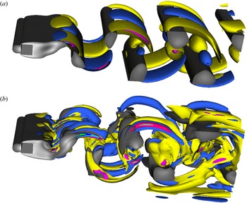
regime, which generates tongue-shaped streamwise vortical structures (shown here in figure 2
a) is the first to become unstable at a Reynolds number between 160 and 175 (Williamson Reference Williamson1996b
; Luo, Chew & Ng Reference Luo, Chew and Ng2003; Saha et al.
Reference Saha, Biswas and Muralidhar2003; Luo et al.
Reference Luo, Tong and Khoo2007). At higher Reynolds numbers (between 190 and 250) a second mode, mode
 $B$
regime, which generates rib-like streamwise vortical structures (see figure 2
b), appears and has smaller wavelength
 $\unicode[STIX]{x1D706}/D\simeq 1.2{-}1.4$
(Williamson Reference Williamson1996b
; Luo et al.
Reference Luo, Chew and Ng2003; Saha et al.
Reference Saha, Biswas and Muralidhar2003; Luo et al.
Reference Luo, Tong and Khoo2007). A third instability mode, namely the
 $C$
mode, that has wavelengths intermediate between those of modes
 $A$
and
 $B$
, was also detected at Reynolds numbers above those for either mode
 $A$
or
 $B$
, by performing Floquet stability analysis (Barkley & Henderson Reference Barkley and Henderson1996; Henderson Reference Henderson1997; Robichaux et al.
Reference Robichaux, Balachandar and Vanka1999; Blackburn & Lopez Reference Blackburn and Lopez2003).
The mechanism of the transition process remains controversial. Williamson (Reference Williamson1996a
) suggested an elliptic instability of the vortex cores to explain the transition to the first three-dimensional unstable mode
 $A$
. However, the mode appears to have the largest amplitude outside the region in which elliptic instability theory indicates it should grow (Henderson Reference Henderson1997). Brede et al. (Reference Brede, Eckelmann and Rockwell1996) showed common features between the
 $A$
,
 $B$
modes and three-dimensional transition of free shear flows (Lasheras & Choi Reference Lasheras and Choi1988), and suggested that the mode
 $A$
regime is likely to originate from an instability of the braid region between the primary vortices due to centrifugal forces. Later, Thompson, Leweke & Williamson (Reference Thompson, Leweke and Williamson2001) re-examined the proposed elliptic instability of Williamson (Reference Williamson1996a
) with further evidence showing that the principal physical origin of mode
 $A$
instability can be attributed to an elliptic instability of the vortex cores and that the observed high perturbation amplitudes outside the vortex cores, specifically in the braids, is due to an amplification of the perturbation in the highly strained hyperbolic region between forming vortices. More recently, these possible explanations were rebutted by Luo et al. (Reference Luo, Tong and Khoo2007), where, based on experimental observations, it was proposed that transition to mode
 $A$
regime is likely to be generated from the combination of the stretch effect of the braid region and the deformation of primary vortices, see their explanatory figure 14 (Luo et al.
Reference Luo, Tong and Khoo2007).
To the best of our knowledge, all of these investigations concentrate on the instabilities of the shed vortices. Experimentally it might be difficult to study the small scale changes around transition (that might come before the large scale vortex deformations described), whereas these could be easily identified in a numerical simulation. Furthermore, the available experimental work does not discuss the onset time of the spanwise perturbation in relation to the start of vortex shedding. We propose to use precise numerical simulations to investigate this stage of the transition process. In this paper, we focus on the origin of the process of transition from two-dimensional to three-dimensional structures in the wake of a square cylinder, by characterizing physical mechanisms observed in the wake before and after the onset of vortex shedding using direct numerical simulations. A full computational analysis of three-dimensional unstable modes is also performed in order to contribute new insights to the discussions of the main cause of the transition.
2 Numerical methods
We consider a single-phase flow with constant density and viscosity, respectively denoted by
 $\unicode[STIX]{x1D70C}$
and
 $\unicode[STIX]{x1D707}$
. The flow motion is described by the incompressible Navier–Stokes equations:
 $$\begin{eqnarray}\left.\begin{array}{@{}c@{}}\unicode[STIX]{x1D70C}(\unicode[STIX]{x2202}_{t}\boldsymbol{u}+\boldsymbol{u}\boldsymbol{\cdot }\unicode[STIX]{x1D735}\boldsymbol{u})=-\unicode[STIX]{x1D735}p+\unicode[STIX]{x1D735}\boldsymbol{\cdot }\unicode[STIX]{x1D70F}+\unicode[STIX]{x1D70C}\boldsymbol{f},\\ \unicode[STIX]{x1D735}\boldsymbol{\cdot }\boldsymbol{u}=0,\end{array}\right\}\end{eqnarray}$$
where
 $\boldsymbol{u}$
is the fluid velocity vector with components
 $u$
,
 $v$
,
 $w$
in the streamwise, vertical and spanwise directions respectively.
 $\unicode[STIX]{x1D70F}=\unicode[STIX]{x1D707}[\unicode[STIX]{x1D735}\boldsymbol{u}+\unicode[STIX]{x1D735}\boldsymbol{u}^{\text{T}}]$
is the viscous stress tensor,
 $\boldsymbol{f}$
represents external forces and
 $p$
the pressure. The Navier–Stokes equations are solved using the high-order spectral element code Nek5000 (Fischer, Lottes & Kerkemeier Reference Fischer, Lottes and Kerkemeier2008). The computational domain is decomposed into
 $K$
hexahedral spectral elements upon which the governing equations are written in the weak form and discretized using a Galerkin method. In each element, the solution is approximated by tensor products of
 $N\text{th}$
-order Legendre polynomial Lagrangian interpolants. Exhaustive details are provided elsewhere, e.g. Fischer et al. (Reference Fischer, Lottes and Kerkemeier2008).
The simulations will be analysed using integral flow parameters such as the Strouhal number
 $St=fD/U_{0}$
where
 $f$
is the measured frequency of the vortex shedding in the wake of the cylinder and the spanwise growth rate
 $\unicode[STIX]{x1D714}_{z}$
. The frequency
 $f$
is extracted by applying a fast Fourier transform algorithm to the time evolution of the streamwise velocity,
 $u$
, recorded at a fixed downstream position situated at
 $0.5D$
behind the cylinder and at the same cross-streamwise position as the top edge of the square cylinder (and at mid-span for the three-dimensional simulations). The necessary minimum dimensionless sampling time of the signal used to obtain an accurate frequency is
 $140$
(corresponding to approximately 20 shedding periods). The growth rate
 $\unicode[STIX]{x1D714}_{z}$
of the spanwise instability is computed as the slope in a log plot of the amplitude of
 $w$
as a function of time. As the spanwise perturbation is quantitatively analysed in the literature using the corresponding Floquet multiplier
 $\unicode[STIX]{x1D707}=\exp (\unicode[STIX]{x1D714}_{z}/f)$
(e.g. Henderson Reference Henderson1997; Robichaux et al.
Reference Robichaux, Balachandar and Vanka1999; Sheard et al.
Reference Sheard, Fitzgerald and Ryan2009),
 $\unicode[STIX]{x1D707}$
is computed in the present work before and after the vortex shedding event occurs, for the sake of comparison. For calculations of the Floquet multiplier before the vortex shedding, we use the frequency
 $f$
of the vortex shedding of the same computation (albeit at a later time) as a non-dimensionalization parameter for consistency.
3 Two-dimensional numerical simulations
The size of the simulation domain is
 $L=40D$
in the streamwise direction with a height denoted
 $H$
. No-slip boundary conditions are applied on the top and bottom edges of the domain. A parabolic velocity profile,
 $(U_{0}[1-(y-0.5H)^{2}/(0.5H)^{2}],0,0)$
where
 $y$
is the cross-streamwise position and
 $U_{0}$
the maximum velocity, is prescribed at the domain inlet and used to initialize the calculations in order to simulate a fully developed laminar channel flow upstream of the square cylinder. However, preliminary simulations with a plug flow velocity profile have shown no significant difference in the dynamics of the flow. The centre of the square cylinder is situated at a streamwise distance of
 $8.5D$
from the domain inlet and vertically in the middle of the domain. Two dimensionless numbers are used to characterize the numerical simulations, namely the Reynolds number
 $Re=\unicode[STIX]{x1D70C}DU_{0}/\unicode[STIX]{x1D707}$
, and the Strouhal number
 $St$
. A Reynolds number range between 100 and 300 is considered.
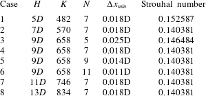
Comparison of the Strouhal number for
 $Re=200$
in flow past a square cylinder, obtained from the present two-dimensional numerical simulations for five different domain heights
 $H$
, and at three different mesh resolutions (numbers of spectral elements
 $K$
, polynomial orders
 $N$
and corresponding minimum mesh spacing
 $\unicode[STIX]{x0394}x_{min}$
).

Two-dimensional simulations have been performed in order to check the effect of the size of the domain and the mesh independence. Different domain heights
 $H=5D,7D,9D,11D,13D$
are used and different polynomial orders
 $N=5,7,9,11$
are applied for a fixed domain height
 $H=9D$
. The Strouhal number corresponding to the dominant frequency
 $f$
of the streamwise vortex shedding is compared at
 $Re=200$
and reported in table 1. As shown in table 1 the Strouhal number remains unchanged from a height
 $H=7D$
and a polynomial order
 $N=7$
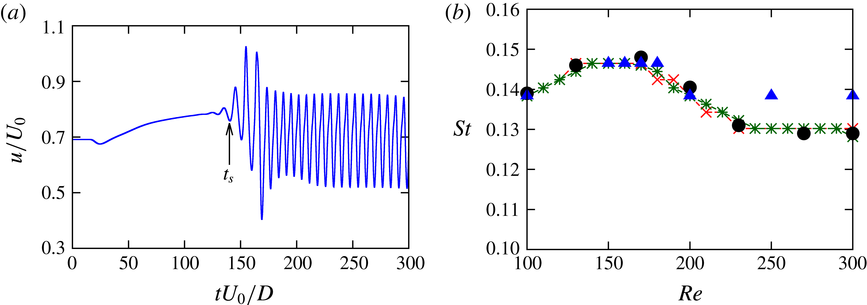
. Figure 1 shows the Strouhal number–Reynolds number relationship obtained from twenty different two-dimensional simulations for
 $H=9D$
and
 $N=7,9$
corresponding respectively to cases 4 and 5 in table 1. Good agreement is obtained with results of Breuer et al. (Reference Breuer, Bernsdorf, Zeiser and Durst2000). Strouhal numbers obtained in three-dimensional simulations (described hereafter) follow the same trend as in two-dimensional simulations up to
 $Re=200$
and become larger for higher Reynolds numbers where the flow is three-dimensional. The maximum error of the obtained shedding Strouhal number–Reynolds number relationship compared to data from Breuer et al. (Reference Breuer, Bernsdorf, Zeiser and Durst2000) (where a minimum mesh spacing
 $\unicode[STIX]{x0394}x_{min}=0.01D$
is used) is approximately 2 % for the two spatial resolutions used, which indicates that the streamwise shedding is not mesh dependent for the considered Reynolds number range.
(a) Time evolution of the streamwise velocity,
 $u$
, for
 $Re=200$
(
 $t_{S}=140$
represents the onset time of the shedding). (b) Comparison of the obtained Strouhal number–Reynolds number relationship for flow past a square cylinder with results of Breuer et al. (Reference Breuer, Bernsdorf, Zeiser and Durst2000) (black ●), present two-dimensional simulations with
 $(K,N)$
:
 $(658,7)$
red
 $\times$
,
 $(658,9)$
dark green
 $\ast$
and present three-dimensional simulations blue ▵.

4 Three-dimensional numerical simulations
For three-dimensional simulations, a spatial mesh in the
 $x-y$
plane corresponding to case 4 in table 1 is used. This two-dimensional grid is then extruded in the spanwise direction for a spanwise length
 $S$
and periodic boundary conditions are imposed in the spanwise direction. Sohankar, Norberg & Davidson (Reference Sohankar, Norberg and Davidson1999) and Saha et al. (Reference Saha, Biswas and Muralidhar2003) have used different values of
 $S$
, namely
 $S=6D,10D$
, and concluded that the physical description of the events following the transition to three-dimensionality does not depend on the spanwise length even though it could affect the transition Reynolds number. First, simulations are performed without imposing upstream disturbances and transition is promoted by discretization errors arising from the governing equations along with those from the boundary conditions. Three-dimensional modes observed in these computations can be thought of as being natural, rather than forced. Then, simulations with upstream perturbations are also performed in order to study the growth of unstable modes.
4.1 Naturally observed three-dimensional modes
In order to minimize the computational cost and to simulate at least one wavelength,
 $S=6D$
is used in the following simulations. Note that the largest wavelength of the unstable transition modes is between
 $5D-5.8D$
(Henderson Reference Henderson1997; Robichaux et al.
Reference Robichaux, Balachandar and Vanka1999; Blackburn & Lopez Reference Blackburn and Lopez2003; Luo et al.
Reference Luo, Chew and Ng2003, Reference Luo, Tong and Khoo2007). Three-dimensional simulations are performed with the same inflow velocity and Reynolds numbers range as in the previous two-dimensional computations. Simulations with a plug flow velocity profile prescribed at the inflow are also performed in three-dimensions in preliminary studies and have shown no significant difference with the following description of the wake dynamics. The tongue-shaped vortex structure with a long spanwise wavelength, characteristic of the mode
 $A$
instability, is observed at
 $Re=180$
(as shown in figure 2
a) while a rib-like vortex structure with a smaller wavelength, characteristic of the mode
 $B$
regime, is observed at
 $Re=300$
(as shown in figure 2
b).
Iso-contours at
 $tU_{0}/D=200$
of positive (yellow) and negative (blue) streamwise vorticity in the wake of the square cylinder showing (a) the tongue-shaped vortical structure of the mode
 $A$
at
 $Re=180$
and (b) the rib-like vortical structure of the mode
 $B$
at
 $Re=300$
. Iso-contours of the velocity magnitude are also displayed in grey colours.

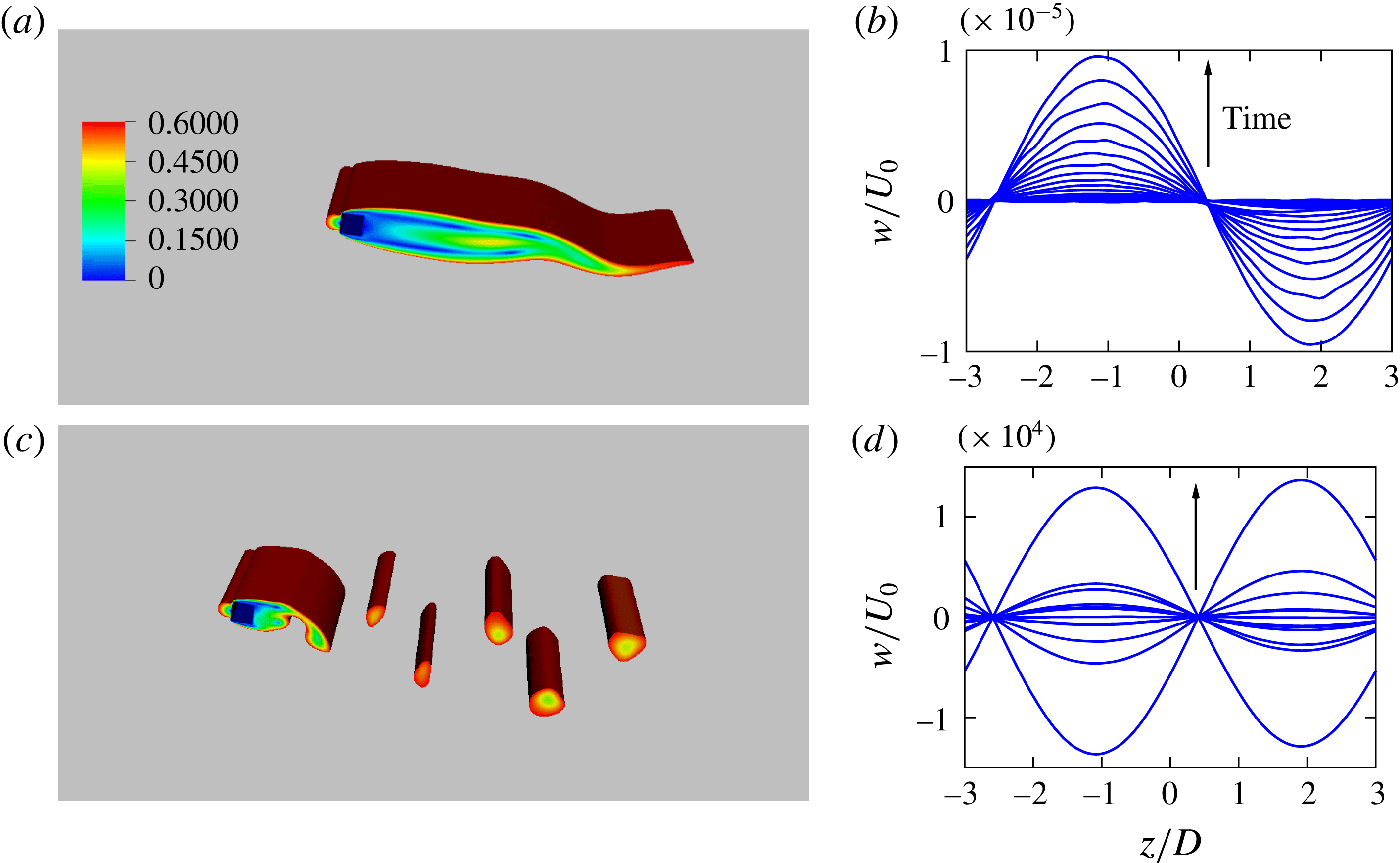
Figure 3(a,c) show iso-contours of the velocity magnitude in the cylinder wake at two different times for
 $Re=200$
. At small time, prior to the vortex shedding event, a cross-stream flapping is observed as shown in figure 3(a). The origin of the flapping is indeed a shear instability which results from the tangential velocity difference between the low-speed fluid sheet in the wake, formed due to the blockage by the cylinder, and a faster stream on the top and bottom sides of the cylinder. The spanwise velocity,
 $w$
, is recorded at
 $0.5D$
downstream of the square cylinder and
 $y=H/2$
and shown in figure 3(b,d). These figures exhibit a sinusoidal perturbation with a fixed wavelength before and after the streamwise vortex shedding occurs. The onset time of the vortex shedding (hereafter denoted by
 $t_{S}$
) is taken as the time where the first oscillations are observed in the streamwise velocity
 $u$
and is shown in figure 1(a) where
 $t_{S}=140$
. The amplitude of
 $w$
is computed using a fit with a sinusoidal function. The amplitude increases with time and oscillations are observed at large time after the vortex shedding, as a consequence of the spatio-temporal symmetry of the wake (Blackburn & Lopez Reference Blackburn and Lopez2003; Blackburn et al.
Reference Blackburn, Marques and Lopez2005). Three different polynomial orders are used for simulations at
 $Re=200$
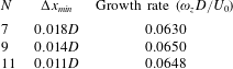
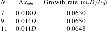
in order to verify the refinement independence of three-dimensional dynamics. As shown in table 2,
 $\unicode[STIX]{x1D714}_{z}$
has approximately the same values for
 $N=7,9,11$
.
Iso-contours of the velocity magnitude for flow past a square cylinder for
 $Re=200$
at
 $tU_{0}/D=130$
(a), showing the flapping of the cylinder wake, and at
 $tU_{0}/D=186$
(c), showing the streamwise vortex shedding. The spanwise velocity
 $w$
, recorded at
 $0.5D$
downstream of the square cylinder and
 $y=H/2$
, is plotted every
 $tU_{0}/D=5$
, during the flapping with
 $5<tU_{0}/D<140$
(b) and after the vortex shedding with
 $180<tU_{0}/D<240$
(d).

Growth rates
 $\unicode[STIX]{x1D714}_{z}$
of the spanwise perturbation in flow past a square cylinder at
 $Re=200$
obtained using three different polynomial orders
 $N$
for a fixed domain height
 $H=9D$
, with the corresponding minimum mesh spacing
 $\unicode[STIX]{x0394}x_{min}$
.
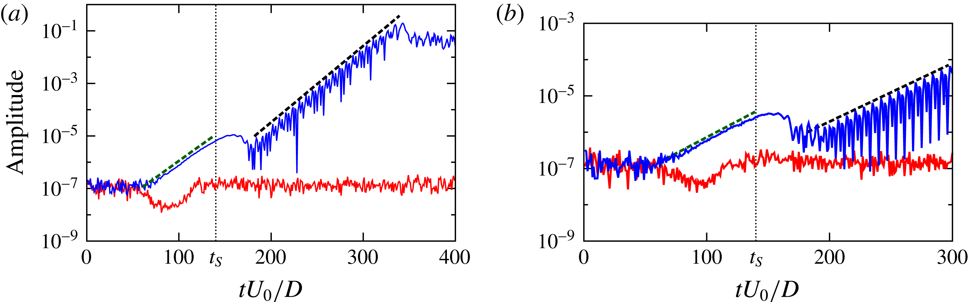
The amplitude of the spanwise perturbation is shown in figure 4 for four different Reynolds numbers. As shown in this figure, the amplitude increases exponentially for
 $Re=180,200$
, while it remains almost constant at
 $10^{-7}$
(corresponding to the amplitude of numerical noise around the null spanwise component of velocity) for
 $Re=\text{150,170}$
. An exponential growth for an order of magnitude between one and two is observed for
 $Re=180,200$
at time smaller than
 $t_{S}$
. It is clear from figures 3 and 4 that the spanwise perturbation occurs before the streamwise vortex shedding. Consequently, interactions of shed vortices or the elliptic instability of the shed vortex cores, as previously observed (Williamson Reference Williamson1996a
; Blackburn et al.
Reference Blackburn, Marques and Lopez2005; Luo et al.
Reference Luo, Tong and Khoo2007), are subsequent to the three-dimensionality of the flow.
As shown in figure 4(b), an exponential growth is observed at
 $Re=180$
while the amplitude remains constant at
 $Re=170$
and for lower values. Transition to three-dimensionality in our simulations is then situated between Reynolds numbers of 170 and 180, which agrees very well with reported experimental and numerical transition Reynolds number ranges, namely 160–175 (Saha et al.
Reference Saha, Biswas and Muralidhar2003; Luo et al.
Reference Luo, Tong and Khoo2007).
Amplitude of the spanwise perturbation as a function of non-dimensional time for flow past a square cylinder for: (a)
 $Re=150$
(red line) and
 $Re=200$
(blue line) and (b)
 $Re=170$
(red line) and
 $Re=180$
(blue line). The dashed black lines correspond to an exponential fit after the vortex shedding, (a)
 $5\times 10^{-11}\exp (0.063tU_{0}/D)$
and (b)
 $1.2\times 10^{-9}\exp (0.037tU_{0}/D)$
. The dashed green lines correspond to an exponential fit before the vortex shedding, (a)
 $3.4\times 10^{-9}\exp (0.058tU_{0}/D)$
and (b)
 $1.2\times 10^{-8}\exp (0.041tU_{0}/D)$
. The onset time
 $t_{S}$
of the vortex shedding is indicated by the small dotted vertical line.

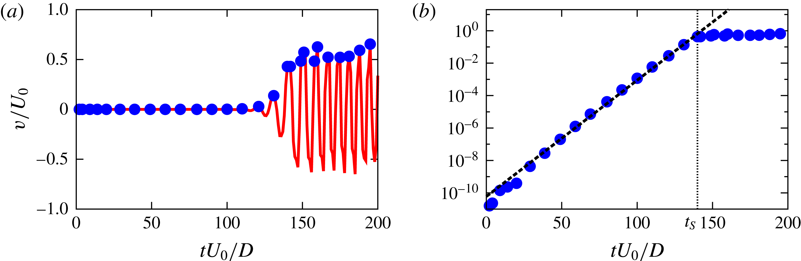
Next, we characterize the cross-stream flapping of the flow by computing its amplification in time. In order to achieve this, the cross-stream velocity,
 $v$
, is recorded as a function of time at downstream positions situated on the centre line
 $y=H/2$
, and
 $z=\text{S}/2$
. As shown in figure 5(a) the obtained oscillating signal increases in time with a wavy envelope which displays local positive maxima and negative minima. The positive maxima are shown by blue dots in figure 5(a) and plotted on a log scale in figure 5(b). An exponential growth is observed up to a time close to
 $t_{S}$
and a saturation is observed afterward.
Note that, the occurrence of the vortex shedding event is accompanied by a decrease and a short stabilization of the amplitude of
 $w$
as shown in figure 4 close to
 $t_{S}$
which also corresponds to the time where the amplitude of the flapping becomes saturated, e.g. see figure 5(b).
Characterization of the flapping instability in flow past a square cylinder. (a) Time evolution at
 $Re=180$
of
 $v/U_{0}$
at the position
 $(18D,H/2,\text{S}/2)$
. The blue points correspond to local maxima of waves along the curve. (b) Log plot (of the same data as in panel a) and fit with exponential function
 $6\times 10^{-11}\exp (0.165tU_{0}/D)$
(black dashed line).

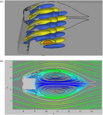
Initial stage (
 $tU_{0}/D=30$
) of the formation of the streamwise vortical structures in the square cylinder wake for
 $Re=300$
. (a) Iso-contours of the vorticity showing the stretching of localized upstream vorticity perturbation. A slice of the spanwise vorticity contours is also shown in the plane
 $z=-3$
. (b) Slice at mid-span of the streamlines (the colour map is the same as in figure 7) and the spanwise (dashed white lines) and the streamwise (dashed black lines) vorticity contours. The streamwise vortices are pulled in downstream from the top and bottom of the square cylinder due the strain field.

4.2 Mechanism of the transition to three-dimensionality
We analyse the onset of the vortical structures by observing the flow features at small times where coherent vortical structures first appear in the cylinder wake. Figure 6(a) shows the streamwise vorticity and a slice of the spanwise vorticity in the wake of the cylinder at
 $tU_{0}/D=30$
for
 $Re=300$
. For the same time and Reynolds number, a cross-stream slice of the streamlines and contours of the streamwise (in dashed black lines) and the spanwise (in dashed white lines) vortices are shown in figure 6(b) at mid-span of the cylinder. First, a double shear layer is formed in the wake once the flow passes the cylinder. The vorticity sheet arising from the cylinder (shown in black lines in figure 6
a) is redistributed into the cores of the spanwise vortices and the braids, connecting the cores of the spanwise vortices and the separation points at the front leading edges of the cylinder, under the effects of the Kelvin–Helmholtz instability. As the evolving spanwise vorticity increases it develops a strain field in the braids which pulls up small localized upstream disturbances and forms regions of concentrated streamwise vortices as shown in figure 6(a,b). Under the shearing effects of the wake, these streamwise vortices are further subjected to stretching along the extensional strain direction. Subsequently, the curved shape of the streamwise vortices (e.g. see figure 2) arises due to the cross-stream flapping of the wake. It is worth noticing that the same three-dimensional instability mechanism was observed numerically, see for instance Pierrehumbert & Widnall (Reference Pierrehumbert and Widnall1982), and experimentally, e.g. Lasheras & Choi (Reference Lasheras and Choi1988), in a plane free shear layer flow. This is consistent with observations by Brede et al. (Reference Brede, Eckelmann and Rockwell1996) suggesting that a similar mechanism of three-dimensional transition may be in play for both flow fields.
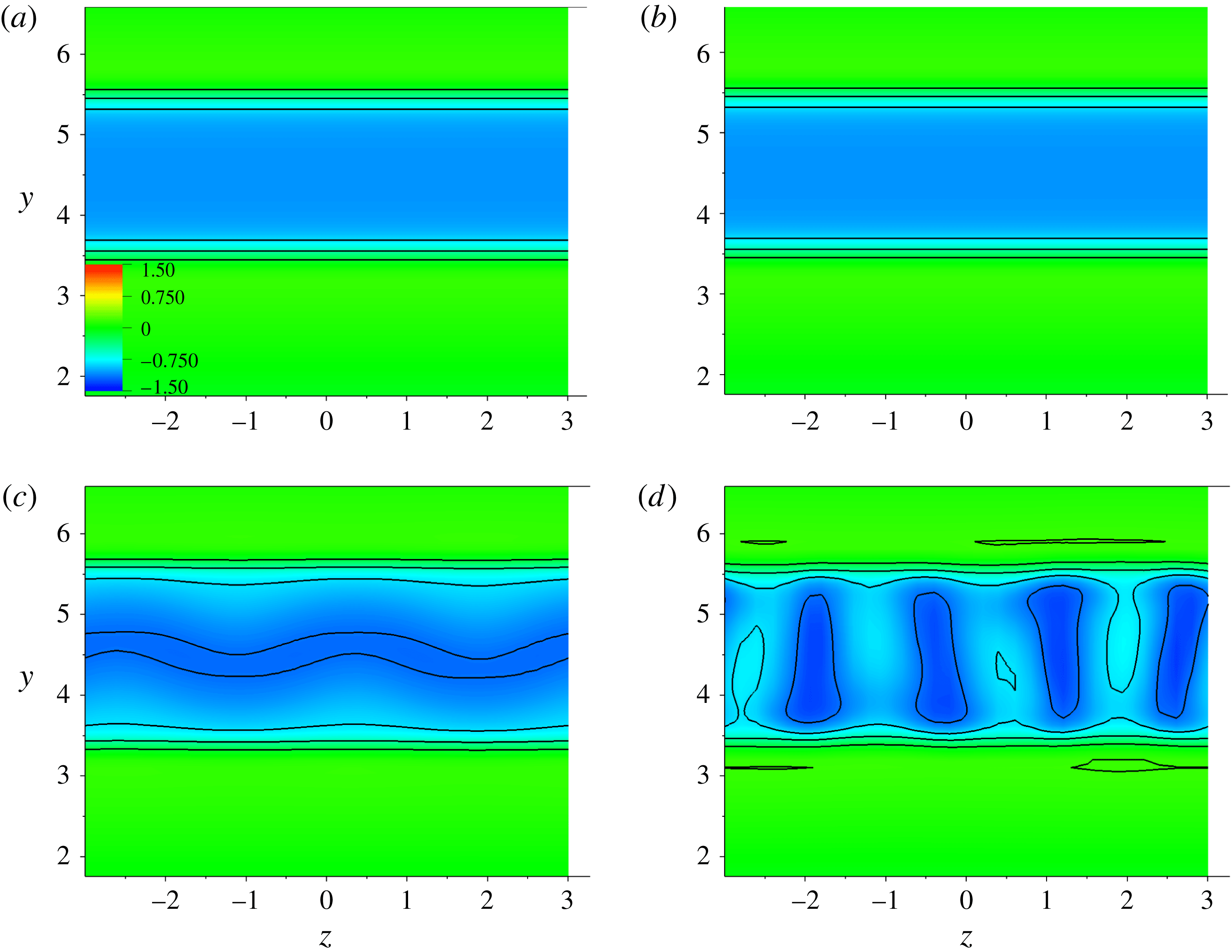
Slices in the spanwise direction at
 $0.5D$
downstream of the square cylinder showing the contours and the magnitudes of the streamwise velocity
 $u2=u-U_{0}$
for
 $Re=200$
(a,b) and
 $Re=300$
(c,d). The images are plotted before the vortex shedding at time
 $tU_{0}/D=100$
in (a) and (c) and
 $tU_{0}/D=120$
in (b) and (d). A vertical instability is observed in the spanwise direction for
 $Re=300$
but not for
 $Re=200$
. The square cylinder is situated between 4 and 5 on the
 $Y$
-axis.

As we proceed in time, a vertical instability is observed in the spanwise direction for
 $Re=300$
(corresponding to the mode
 $B$
regime) before the vortex shedding. Interestingly, this vertical instability does not appear at
 $Re=200$
(corresponding to the mode
 $A$
regime) as shown in figure 7 where slices of the streamwise velocity in a reference frame moving with the mean flow,
 $u2=u-U_{0}$
, are shown for
 $Re=200$
in figure 7(a,b) and for
 $Re=300$
in figure 7(c,d) at
 $tU_{0}/D=100,120$
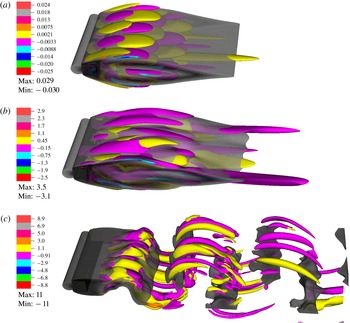
. As the vertical instability increases the flow in the near wake becomes nonlinear and interacts with the previously formed vortical structures before spanwise vortices are shed, see figure 8(b). Then, the resulting nonlinear wake reorganizes into the rib–like vortex shapes with a small wavelength corresponding to the mode
 $B$
regime once the vortex shedding is initiated.
Iso-contours of the streamwise vorticity field in the cylinder wake for
 $Re=300$
. The time sequence
 $tU_{0}/D$
is from the top to bottom, (a)
 $80$
, (b)
 $120$
, (c)
 $250$
. The wake becomes nonlinear in the image (b), before the vortex shedding, due to the vertical instability shown in figure 7. Iso-contours of the velocity magnitude are also displayed in grey colours.

4.3 Three-dimensional unstable modes of the perturbed wake
The perturbed wake is studied in this section in order to validate the observation that the cylinder wake is unstable to three-dimensional perturbation before the vortex shedding occurs and to check that the observed instabilities, before and after the vortex shedding, have the same maximum unstable mode. To do so, a three-dimensional disturbance is imposed at the inflow on two different initial velocity conditions, namely a steady flow as in the previous § 4.1 and a periodic flow where the wake is subjected to periodic vortex shedding.
First, a sinusoidal perturbation with fixed wavenumbers corresponding to each previously reported three-dimensional modes (
 $A$
,
 $B$
and
 $C$
) is imposed on the two-dimensional steady inflow prior to the vortex shedding so that the growth or the stabilization of the perturbation before and after the vortex shedding can be observed. Second, growth rates are calculated for the same perturbation with spanwise wavenumbers varied between 0.5 and 8 where unstable modes in the wake have been predicted (Robichaux et al.
Reference Robichaux, Balachandar and Vanka1999; Sheard et al.
Reference Sheard, Fitzgerald and Ryan2009). Then, the computed growth rates are compared to the stability analysis of Robichaux et al. (Reference Robichaux, Balachandar and Vanka1999) in which the perturbation is imposed on the two-dimensional periodic wake obtained after the streamwise vortex shedding occurs.
4.3.1 Perturbation added to the two-dimensional steady flow prior to the vortex shedding
A divergence-free sinusoidal perturbation is now imposed on the inlet velocity in the form:
 $$\begin{eqnarray}\displaystyle (-A_{0}U_{0}xk_{z}\cos (k_{z}z),A_{0}U_{0}\cos (k_{z}z),A_{0}U_{0}\sin (k_{z}z)), & & \displaystyle\end{eqnarray}$$
where
 $A_{0}$
is the initial amplitude of the perturbation. The spanwise length of the computational domain
 $S$
is varied from
 $3D$
to
 $11D$
and a single or multiple wavelengths of the same mode are imposed in order to simulate a particular wavenumber
 $k_{z}$
. Simulations are performed at
 $Re=205$
with wavenumbers corresponding to each of the transition modes:
 $k_{z}D=1.047$
for the mode
 $A$
,
 $k_{z}D=2.09$
for the mode
 $C$
and
 $k_{z}D=6.28$
for the mode
 $B$
, e.g. see Robichaux et al. (Reference Robichaux, Balachandar and Vanka1999). The initial amplitude of the perturbation is fixed at
 $A_{0}=10^{-5}$
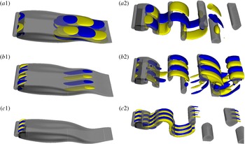
. Three-dimensional iso-surface plots of the vorticity magnitude in the cylinder wake are shown in figure 9 at small time before the vortex shedding (a1,b1,c1) and at large time (a2,b2,c2).
Figure 9(a1,a2) shows the computed wake for
 $k_{z}D=1.047$
(corresponding to a wavelength
 $\unicode[STIX]{x1D706}_{z}=2\unicode[STIX]{x03C0}D/k_{z}=6D$
). The observed structures in the wake exhibit a spatio-temporal symmetry by evolving the wake by one half-period and reflecting about the centre line (a half-period flip). This is characteristic of the mode
 $A$
instability (Henderson Reference Henderson1997).
For
 $k_{z}D=2.09$
, corresponding to
 $\unicode[STIX]{x1D706}_{z}=3D$
, the structures in the wake are consistent with the quasi-periodic mode
 $C$
. Figure 9(b1,b2) shows a half-period flip as in the case of the mode
 $A$
but with a smaller wavelength.
In figure 9(c2), where
 $k_{z}D=6.28$
(
 $\unicode[STIX]{x1D706}_{z}=1D$
), a half-period flip and a spanwise translation of half the wavelength of the mode recovers the original flow. This is consistent with the mode
 $B$
instability. It is notable that in figure 9(a1,a2) and in figure 9(b1,b2) corresponding respectively to the mode
 $A$
and the mode
 $C$
instabilities, vortical structures are visible in the wake before and after the vortex shedding while for the mode
 $B$
instability shown in figure 9(c1,c2), vortical structures are observed in the wake only after the vorticity is shed. This is consistent with the above observation that the spanwise perturbation occurs in the wake before the streamwise vortex shedding for wavenumbers corresponding to the instability modes
 $A$
and
 $C$
. However, figures 9(c1,c2) suggest that the wake is unstable for wavenumbers corresponding to the mode
 $B$
only after the vortex shedding. To validate this, growth rates are calculated for perturbations with spanwise wavenumbers
 $k_{z}D$
varied between 0.5 and 8.
Iso-contours of the positive (yellow) and negative (blue) streamwise vorticity in the wake of the square cylinder for
 $Re=205$
before the vortex shedding at
 $tU_{0}/D=120$
(a1,b1,c1) and in the shedding regime at
 $tU_{0}/D=207$
(a2,b2,c2). Each pair (left–right) is drawn to the same scale. The wavenumbers in the upstream perturbation are
 $k_{z}D=1.047$
for images (a1) and (a2) showing the mode
 $A$
instability,
 $k_{z}D=2.09$
for images (b1) and (b2) showing the mode
 $C$
instability and
 $k_{z}D=6.28$
for images (c1) and (c2) showing the mode
 $B$
instability. The wake is stable during the flapping regime in (c1) and no vortical structures are present. Iso-contours of the velocity magnitude are also displayed in grey colours.

The amplitude of the perturbation is computed based on the spanwise velocity which is recorded in time at the same location as previously,
 $0.5D$
downstream of the square cylinder and
 $y=H/2$
. For the sake of generality, the
 $L_{2}$
norm of the spanwise velocity:
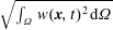 $\sqrt{\int _{\unicode[STIX]{x1D6FA}}w(\boldsymbol{x},t)^{2}\,\text{d}\unicode[STIX]{x1D6FA}}$
, where
 $\unicode[STIX]{x1D6FA}$
represents the simulation domain and
 $\boldsymbol{x}$
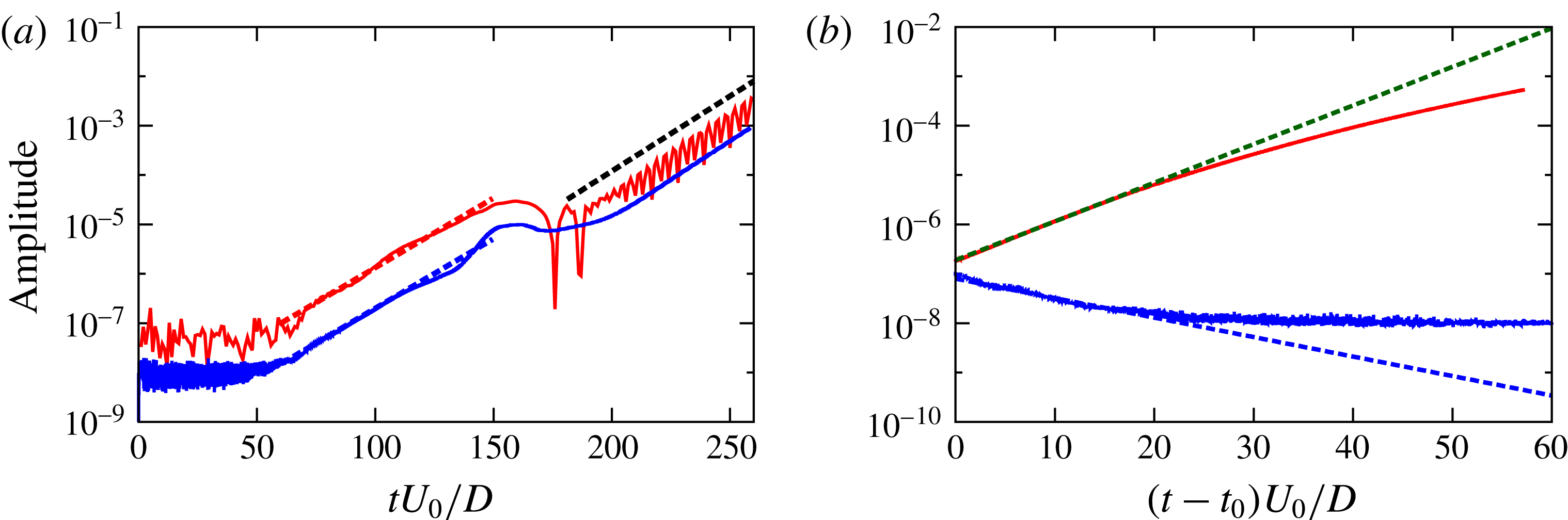
the position vector, is also used to monitor the amplitude of the perturbation and to check the non-dependence on space of the growth of the amplitude. Figure 10(a) shows both calculations of the amplitude as a function of time in a preliminary simulation for
 $Re=205$
and
 $\unicode[STIX]{x1D706}_{z}=6D$
, without imposing the upstream perturbation. In this figure, the slope of the amplitude is approximately the same before and after the vortex shedding is initiated, for both calculations. However, the localized amplitude calculation, red line in figure 10(a), is more noisy between time 70 and 100 than for the
 $L_{2}$
norm. Note also that in figure 10(a) the amplitude is smaller by approximately one order of magnitude when using the
 $L_{2}$
norm. This is expected as the integral in the
 $L_{2}$
norm is calculated over the whole domain while the perturbation grows only in the cylinder wake. The
 $L_{2}$
norm is used to compute the amplitude in the rest of the study.
Amplitude of the spanwise velocity as a function of time for
 $Re=205$
. (a) Two different calculations of the amplitude for a simulation with no upstream perturbation: using a fit of the recorded velocity at a fixed location in the wake with a sinusoidal function (red line) and using the
 $L_{2}$
norm of
 $w$
(blue line). Exponential fits are shown in dashed lines: before the vortex shedding
 $3\times 10^{-10}\exp (0.065tU_{0}/D)$
(in blue) and
 $2\times 10^{-9}\exp (0.065tU_{0}/D)$
(in red) and after the vortex shedding
 $1\times 10^{-10}\exp (0.07tU_{0}/D)$
(in black). (b) Obtained amplitude, using the
 $L_{2}$
norm, for upstream perturbations with
 $A_{0}=10^{-7}$
for two different wavenumbers
 $k_{z}=1.047$
(red line) and
 $k_{z}=4.724$
(blue line). The dashed lines correspond to exponential fits.

Simulations with upstream perturbations are conducted for two different Reynolds numbers
 $Re=205,225$
and for different three-dimensional instability modes in order to check their growth or stabilization before the vortex shedding occurs, i.e. for
 $tU_{0}/D<t_{S}\simeq 140$
. Figure 10(b) shows examples of the calculated amplitude of the perturbation as a function of time for an initial amplitude
 $A_{0}=10^{-7}$
, and two different wavenumbers
 $k_{z}=1.047,4.724$
. In this figure, a transient time
 $t_{0}$
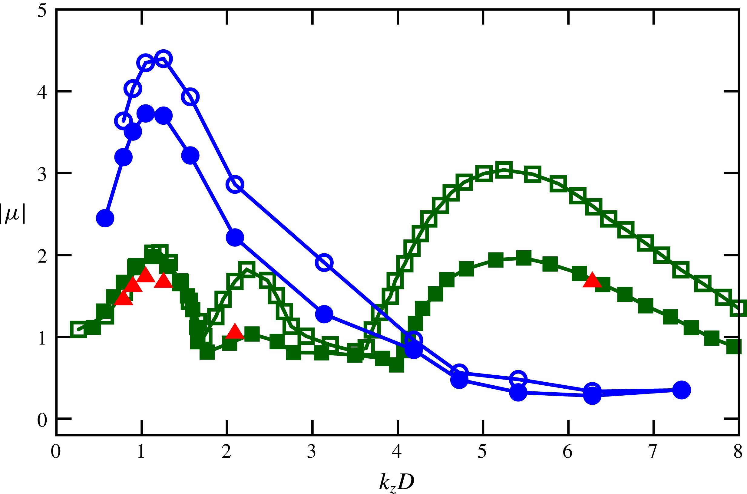
, which corresponds to the time it takes for the flow to travel from the inlet to the back of the cylinder, is removed from the considered time for the exponential growth. However, the amplitude grows exponentially only for a short time, by approximately one order of magnitude, and then becomes saturated. Figure 11 shows the obtained Floquet multipliers (defined in § 2). Floquet multipliers obtained in Robichaux et al. (Reference Robichaux, Balachandar and Vanka1999) (see their figure 8) were digitized and included in figure 11 along with the present results. It is clearly shown that the wake is unstable (i.e.
 $|\unicode[STIX]{x1D707}|>1$
) when wavenumbers corresponding to the mode
 $A$
and the mode
 $C$
are imposed in the upstream perturbation while it stabilizes for wavenumbers corresponding to the mode
 $B$
. In figure 11 even though Floquet multipliers obtained in the simulations (before the vortex shedding occurs) are much larger than in the Floquet stability analysis (performed using a base velocity recorded for one period of shedding in a two-dimensional simulation), the peak of the high-wavenumber mode is achieved at a wavenumber between
 $1.047$
and
 $1.256$
, so approximately at
 $k_{z}D\simeq 1.15$
which is very close to the reported high-wavenumber value
 $k_{z}D\simeq 1.14$
(Robichaux et al.
Reference Robichaux, Balachandar and Vanka1999) of the mode
 $A$
. This suggests that the wake is at least unstable to the mode
 $A$
before the vortex shedding occurs.
Floquet multiplier magnitude
 $|\unicode[STIX]{x1D707}|$
as a function of spanwise wavenumber. The open symbols correspond to
 $Re=225$
and filled symbols to
 $Re=205$
. Floquet multipliers obtained at small time before the vortex shedding occurs are shown in blue circles
 $\circ$
and those at large time after the shedding is initiated in red triangles ▵. Data from Robichaux et al. (Reference Robichaux, Balachandar and Vanka1999) are indicated by green squares ▫.

4.3.2 Perturbation added to the periodic two-dimensional wake after the vortex shedding occurs
Additionally, simulations are performed at
 $Re=205$
for different wavenumbers, with the difference that, the upstream perturbations are now imposed only after the streamwise vortex shedding has occurred. Note that this methodology is similar to the way the Floquet stability analysis was carried out (Henderson Reference Henderson1997; Robichaux et al.
Reference Robichaux, Balachandar and Vanka1999; Sheard et al.
Reference Sheard, Fitzgerald and Ryan2009). As shown in figure 11 (by red triangles), the Floquet multipliers obtained using this methodology in the simulations agree well with the stability analysis results (e.g. Robichaux et al.
Reference Robichaux, Balachandar and Vanka1999). Interestingly the cylinder wake is now unstable for
 $k_{z}D=6.28$
corresponding to the mode
 $B$
regime. This is coherent with the above observation that the mode
 $B$
is triggered after the spanwise vorticity has been shed.
5 Conclusion
We performed direct numerical simulations of flow past a square cylinder using a high-order spectral element method. The obtained Strouhal number–Reynolds number relationship is validated by previous works (Breuer et al. Reference Breuer, Bernsdorf, Zeiser and Durst2000) and the Reynolds number range for transition to three-dimensionality agreed well with previous simulations and experimental observations.
Beyond the transition, a sinusoidal perturbation was observed on the spanwise velocity. This perturbation occurred prior to the streamwise vortex shedding and the amplitude of the perturbation increases by approximately two orders of magnitude before the onset of the shedding, at times where the cylinder wake is subjected to a cross-streamwise flapping due to the double shear layer formed in the near wake. The first transition mode, the mode
 $A$
, is observed to originate from an axial stretching of upstream small perturbations due to a strain field created by spanwise vortices which form and evolve in the near wake under a shear instability once the flow passes the cylinder. On the other hand, the mode
 $B$
is formed only after the streamwise vortex shedding occurs. At a Reynolds number
 $Re=300$
corresponding to the mode
 $B$
, a vertical instability in the spanwise direction is observed in the wake. This instability grows rapidly and interacts with the existing streamwise vortices in the wake before the vortex shedding occurs. The resulting nonlinear wake alters the base flow characteristics and forms vortical structures corresponding to the mode
 $B$
once the vortex shedding is initiated.
Simulations with upstream perturbations were conducted and the predicted three-dimensional unstable modes in the wake (Robichaux et al.
Reference Robichaux, Balachandar and Vanka1999; Blackburn & Lopez Reference Blackburn and Lopez2003; Sheard et al.
Reference Sheard, Fitzgerald and Ryan2009) were observed. At small time, before the vortex shedding occurs, the cylinder wake was shown to be unstable to wavenumbers corresponding to the modes
 $A$
and
 $C$
instabilities while it is stable for wavenumbers associated with the mode
 $B$
. The obtained growth rates, at small time, of the unstable wavenumbers are larger, by approximately a factor of two, compared to those obtained in the Floquet stability analysis where a base flow recorded in the vortex shedding regime in a first run two-dimensional simulation was used. Nevertheless, the peak of the high-wavenumber mode, at small time, is achieved at a wavenumber very close to the obtained peak of the mode
 $A$
in the Floquet stability analysis and the growth rates compared better at large time after the vortex shedding occurs. However, the obtained dispersion curve at small time does not exhibit two different peaks for modes
 $A$
and
 $C$
as observed in the Floquet stability analysis. This suggests that at transition the first three-dimensional instability mode, the mode
 $A$
, occurs before the onset of the vortex shedding with large growth rates which later decrease at large time under nonlinear effects, while the modes
 $C$
and
 $B$
arise once the vortex shedding is initiated downstream of the cylinder.
Acknowledgements
The authors thank the Natural Sciences and Engineering Research Council of Canada and the University of Ottawa for financial support, Compute Canada and SciNet for computational support and R. D. Deegan for valuable discussions. This line of inquiry was suggested by R. Vinuesa following our joint work on the wall-mounted square cylinder (Vinuesa et al. Reference Vinuesa, Schlatter, Malm, Mavriplis and Henningson2015).