Introduction
Due to increasing intentional and unintentional electromagnetic interferences (EMI), analyzing the susceptibility of electronic circuits to external electromagnetic (EM) wave illumination has become essential in modern design [Reference Bäckström and Lövstrand1]. The coupling of the incident EM wave to the circuit mainly occurs through open distributed elements, such as transmission lines (TLs), vias, and discontinuities, which act as the receiving antenna. The coupled energy to the TLs can be transferred to the circuit components and, as a result, depending on the power level of the incident field, can disrupt the operation of the circuit or cause physical damage [Reference Bäckström and Lövstrand1, Reference Ott2]. Three of the most common approaches for solving the field to line coupling problem are full-wave analysis based on Maxwell's equations [Reference Tesche, Ianoz and Karlsson3], thin-wire approximation [Reference Leone, Bruns and Singer4], and TL theory [Reference Paul5]. Much of the literature on analyzing the linear terminated TLs subjected to the incident EM field uses the TL theory, which is based on the quasi-transverse EM (TEM) mode assumption [Reference Leone, Bruns and Singer4, Reference Paul5].
Furthermore, with the increasing operating frequencies and integration scale in radio-frequency (RF)/microwave circuits, more attention has been focused on investigating the effect of the incident EM wave coupling to the active nonlinear circuits [Reference Rizzoli, Costanzo and Monti6, Reference Zhang and Wang7]. For accurate analysis of the nonlinear circuit illuminated by the incident EM wave, field to line coupling equations and nonlinear circuit equations must be incorporated and solved simultaneously. This problem can be handled using the finite-difference time-domain (FDTD) method, which is widely utilized for the numerical analysis of linear/nonlinear differential equations due to its simplicity and capability to work with a wide range of excitation sources and frequencies [Reference Paul5, Reference Orlandi and Paul8]. However, the conventional explicit FDTD approach is not very time efficient because the temporal step must be limited by the Courant–Friedrichs–Lewy (CFL) condition to guarantee numerical stability. Consequently, researchers have developed various modified FDTD approaches, such as alternating-direction implicit FDTD [Reference Namiki9] and Crank–Nicholson methods [Reference Sun and Trueman10], to eliminate the CFL stability condition. Nevertheless, most of these approaches are proposed to analyze linearly loaded TLs and do not guarantee unconditional stability for TLs terminated by nonlinear circuits. Furthermore, these unconditional approaches do not attain good accuracy for any time step size.
This paper presents a new unconditionally stable time-domain algorithm for analyzing the nonlinearly loaded TLs excited by the EM wave illumination. In the proposed algorithm, the field to line coupling equations and linear/nonlinear boundary conditions are incorporated and described in a matrix form. Then, the derived differential matrix equations are discretized and solved using the proposed FDTD approach. In this method, a new parameter is defined and used to discretize the derived differential matrix equations, which ensures the stability and accuracy of the proposed method by selecting the optimal value for it. Further, for the TLs with nonlinear termination to avoid instability, the discretized nonlinear matrix equations are solved by applying an iterative globally convergent approach. Moreover, to confirm the accuracy of the proposed method, measurements have been carried out using a TEM cell to investigate a single microstrip line and a power detector circuit, which are excited by the uniform EM field illumination. The proposed method results are also validated by comparing with the analytical results and Advanced Design System (ADS) simulation results in the absence of the incident field illumination. The paper algorithm would be applicable in investigating the effects of the EM and high-power microwave (HPM) pulses [Reference Nitsch, Camp, Sabath, Haseborg and Garbe11] illumination on the nonlinear microwave circuits.
THEORY
In this section, first, the TL equations in the presence of the external incident EM wave are presented. The proposed generalized FDTD method is then applied to solve the equations of a TL with linear terminations. Finally, the solution of the nonlinearly loaded TL equations is derived.
Equations of TLs illuminated by incident EM wave
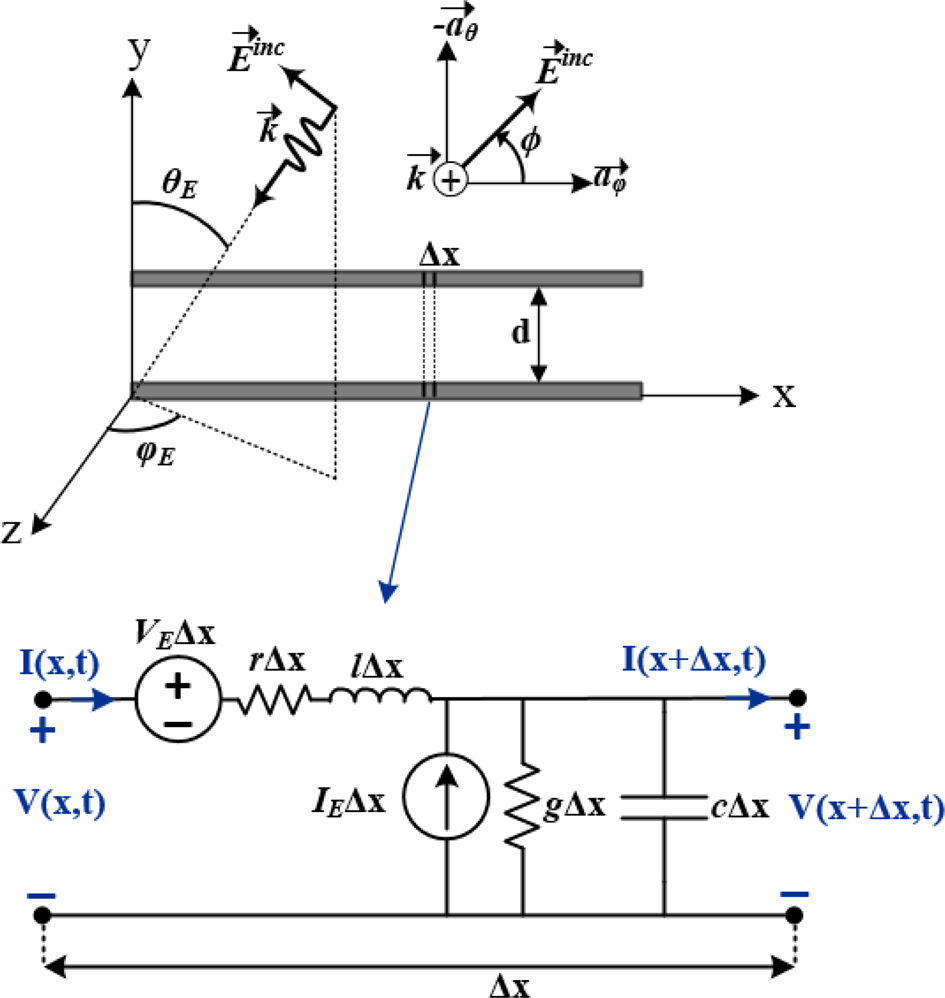
As shown in Fig. 1, the coupling of the external EM wave to a TL is modeled using two additional induced sources in the per-unit-length equivalent circuit model of the line. Therefore, by considering the quasi-TEM approximation, the time-domain equations of a TL excited by the EM wave illumination can be written as follows [Reference Agrawal, Price and Gurbaxani12]:


where l, r, c, and g denote the per-unit-length parameters for the TL. Also, the per-unit-length induced sources due to the EM excitation field (V E and I E) can be obtained from the incident magnetic ($\vec{B}_{inc}$ ) and electric ($\vec{E}_{inc}^t$
 ) fields as follows:


where $\vec{a}_n$ is the unit vector normal to the plane created by the x-axis and the connecting line between the centers of the two conductors of the TL (the x–y plane as shown in Fig. 1). For the uniform plane wave excitation, the electric field can be represented by:

where θ E and φE are the incidence angles, and function f W denotes the waveform of the incident wave. According to Fig. 1, the polarization vector ($\vec{P}$ ) of the incident field can be written as

where ϕ denotes the polarization angle of the electric field. Furthermore, in the case of a TL with a conductor at height d placed above a ground plane and illuminated by the uniform plane wave, the induced sources can be formulated as follows:


It should be noted that these equations are derived by considering the incident filed and reflected field from the ground plane [Reference Paul5].
Modeling of a TL with a conductor at height d placed above a ground plane, which is illuminated by the external incident uniform EM wave with the propagation vector of $\vec{k}$ , incidence angles of θ E and φE, and the polarization angle of ϕ. The per-unit-length inductance, resistance, capacitance, and conductance of the line are denoted by l, r, c, and g, respectively. Also, V E and I E are the per-unit-length induced sources due to the EM excitation field, and V(x, t) and I(x, t) denote the line voltage and current, respectively, as a function of position (x) and time (t).

Generalized FDTD solution method for TLs with linear termination
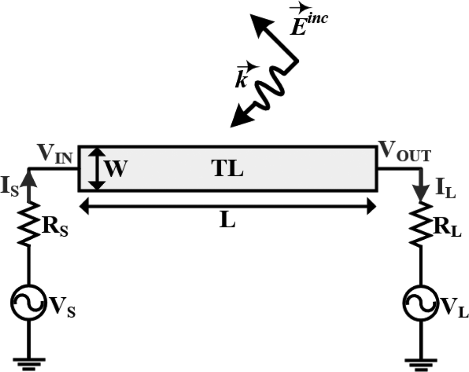
In this subsection, for simplicity, the development of the proposed generalized FDTD approach is presented for a two-conductor TL as shown in Fig. 2. In the proposed method, the forward difference approximation of the spatial derivative is first used to express (1) in discrete space as follows:

where V i ≡ V((i − 1)Δx, t) and I i ≡ I((i − 0.5)Δx, t). Moreover, it is assumed that the line is discretized into N x cells of length Δx. Similarly, using the backward difference approximation of the spatial derivative, equation (2) can be discretized as follows:

Illumination of the incident EM wave to a TL terminated with the linear load.

According to Fig. 2, by using the current–voltage relationships in the source (I S = −V 1/R S + V S/R S) and load ($I_L = V_{N_x + 1}/R_L-V_L/R_L$ ), and replacing Δx ⇒ 0.5Δx in equation (10), the terminal relations (i = 0, i = N x + 1) can be obtained as follows:


By defining the vectors


equation (9) can be written in the matrix form as follows:

wherein:


Equations (10)–(12) can be similarly expressed in the matrix form as follows:

wherein:


The source matrices $\overline {{\bf V}_{\bf S}}$ and $\overline {{\bf I}_{\bf S}}$
 include the line excitation sources and field-to-line coupled sources. Applying the forward difference approximation in the time domain to equations (16) and (20) results in:


where superscript n denotes the time step. In the proposed method, voltage and current vectors are defined as the weighted average over the time step as follows:


where α is the weighting factor (0 ≤ α ≤ 1). It can be observed that the proposed generalized FDTD method with specific values of α leads to the conventional FDTD approaches such as the explicit scheme (α = 0), the Crank–Nicholson scheme (α = 0.5), and the fully implicit scheme (α = 1). Finally, substituting the average vectors (equations (27)–(30)) into equations (25) and (26) gives the final iteration formulas based on proposed generalized FDTD for the voltages and currents of the line shown in Fig. 2, in the matrix form as follows:

wherein:


In order to guarantee the stability of the proposed method, the spectral radius of the square matrix $\bar{{\bf \Phi }}$ (that is the largest absolute value of its eigenvalues) must be less than one ($\rho ( {\bar{{\bf \Phi }}} ) \le 1$
 ) [Reference Kantartzis and Tsiboukis13]. It will be shown in the next section that this condition is satisfied for 0.5 ≤ α ≤ 1, and consequently, the proposed method is unconditionally stable even for arbitrarily large time steps.
Generalized FDTD solution method for nonlinearly loaded TLs
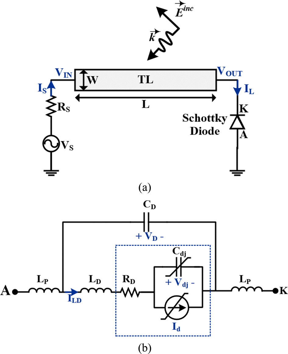
As shown in Fig. 3(a), consider a TL that is terminated with a Schottky diode as a nonlinear load and excited by the external EM wave illumination. For incorporating the nonlinear terminal conditions in the proposed FDTD algorithm, an accurate large-circuit model of the nonlinear device must be used. Thus, the nonlinear lumped-circuit model of the Schottky diode investigated in this paper, which includes the intrinsic part with the nonlinear elements and the extrinsic parasitic elements, is presented in Fig. 3(b). In the PN-junction diode model [Reference Antognetti and Massobrio14], which is used for modeling of the intrinsic part, the nonlinear diode current and capacitor are given by:


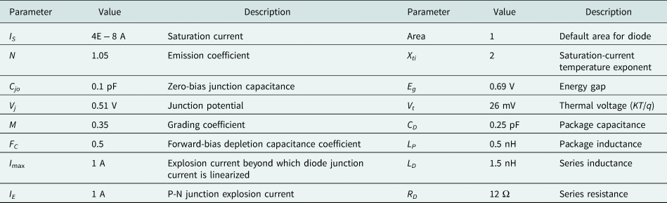
wherein V max = N ⋅ V tLn(I E/I S + 1). Also, I S, I E, N, V t, I max, Area, C jo, V j, M, and F C are the model parameters of the diode, and V dj denotes the internal junction voltage. The descriptions and values of model parameters for the Schottky diode used in this paper are presented in Table 1. Therefore, applying Kirchhoff's law at the nonlinear load termination network shown in Fig. 3 gives the relations for the load terminal as:


(a) Illumination of the incident EM wave to a TL terminated with a diode. (b) The schematic diagram of the large-signal circuit model of the Schottky diode.

Model parameters of the diode SMS7621-001LF.

Moreover, substituting Δx ↠ 0.5Δx and i = N x + 1 into equation (10) gives:

As in the previous subsection, representing equation (10) and the constraint equations, including the nonlinear load termination circuit equations (38)–(40) and source terminal equation (11) together in the matrix form results in:

wherein:


Moreover, equations (9), (36), and (37) can be similarly written in the matrix form as follows:

wherein:


Finally, using the forward difference approximation and substituting the proposed average vectors (equations (27)–(30)) into the time-domain equations (41) and (48), the matrix form of the final recursion relation for the nonlinearly loaded line can be determined as:

where $\bar{{\boldsymbol S}} = \left[{\matrix{ {\bar{{\bf V}}} \cr {\bar{{\bf I}}} \cr } } \right]$ and $\bar{{\boldsymbol U}} = \left[{\matrix{ {\overline {{\bf I}_{\boldsymbol S}} } \cr {\overline {{\bf V}_{\boldsymbol S}} } \cr } } \right]$
 . Also, matrices $\bar{{\bf \Psi }}$
 and $\bar{{\bf \Phi }}$
 are given in (32) and (33), respectively. An iterative root-finding method can be used to solve the nonlinear equation (53). Since locally convergent methods are not converged for any arbitrary initial conditions in the highly nonlinear equations, a globally convergent approach is utilized to ensure the stability and convergence of the presented algorithm. Applying the global Newton method [Reference Kelley15] to solve the nonlinear equation (53) results in:

where the Jacobian matrix of F (${\boldsymbol J} = \partial {\boldsymbol F}( {\bar{{\boldsymbol S}}} ) /\partial \bar{{\boldsymbol S}}$ ) can be obtained as follows:

The parameter $\delta _k^{\rm \ast }$ is called the Newton step and must be obtained in each iteration to ensure the convergence of the proposed method (${\boldsymbol F}( {{\bar{{\boldsymbol S}}}_{{\boldsymbol k} + 1}} ) \ll {\boldsymbol F}( {{\bar{{\boldsymbol S}}}_{\boldsymbol k}} )$
 ).
As mentioned above, the proposed algorithm is applicable in the frequency range that the quasi-TEM mode assumption is satisfied. For the microstrip circuits, the quasi-TEM propagation mode is limited to the cutoff frequency, which is given by [Reference Leone and Singer16]:

where d and ε r are the thickness and relative permittivity of the substrate, respectively, and W denotes the trace width. According to (56), the cutoff frequency range for typical microstrip lines (d/5 ≤ W ≤ 3d, 1 ≤ ɛr ≤ 6) supporting the quasi-TEM mode is 2–10 GHz. Moreover, it is worth noting that the large-signal lumped-circuit models for the nonlinear components are not valid at high frequency since the dimensions of the active devices could not be ignored compared to the wavelength of the incident field. Under these conditions, the distributed TL models [Reference Seifi, Abdipour and Mirzavand17] for nonlinear devices could be used in the presented algorithm.
APPLICATIONS
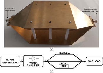
In this section, two examples, including a linearly loaded microstrip TL and a diode detector circuit illuminated by the external uniform EM wave, are investigated to verify the stability and accuracy of the proposed method (see Fig. 4). Furthermore, measurements are carried out using a TEM cell to investigate the effects of external EM field coupling to the microstrip circuits and validate the proposed method. TEM cells are well suited for use in a radiated susceptibility test of the electronic boards and devices in the laboratory because the field produced inside the TEM cell is known with high accuracy [Reference Garcia, Lee and Hagness19].
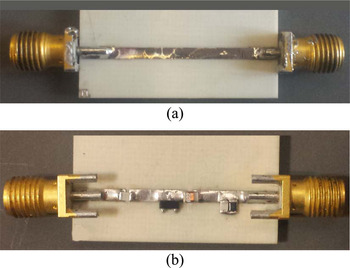
The real photo of (a) the single microstrip line and (b) the power detector circuit implemented on the RO4003 substrate.

The designed and implemented TEM cell for generating the uniform EM wave is shown in Fig. 5(a). As observed in the setup for radiated susceptibility measurement presented in Fig. 5(b), the device under test (DUT) is positioned between the inner and bottom conductors.
(a) Photograph of the fabricated TEM cell. (b) Radiated susceptibility measurement setup.

EM coupling of a single microstrip line with linear termination
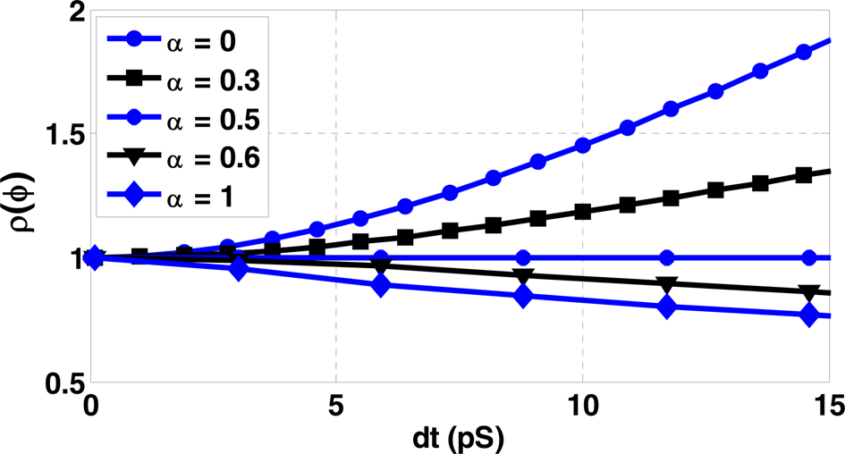
As a first example, a single microstrip TL on the RO4003 substrate (ɛr = 3.38 and d = 0.8 mm) is investigated to validate the proposed method (see Fig. 4(a)). The line has a width of 1.8 mm and a length of 30 mm and is terminated by linear loads. The generalized FDTD method is first applied to analyze the microstrip line without the incident wave, and the terminal conditions are R s = 50 Ω, R L = 50 Ω, and V s = sin(2π109t). The stability of the proposed FDTD method for different values of α is investigated based on the spectral radius of the amplification matrix. The values of $\rho ( {\bar{{\bf \Phi }}} )$ versus the time step are obtained from equation (33), and the results are shown in Fig. 6. It can be observed that the proposed FDTD method for 0.5 ≤ α ≤ 1 is unconditionally stable since, in this case, the spectral radius of the amplification matrix for any time step size is less than or equal to one ($\rho ( {\bar{{\bf \Phi }}} ) \le 1$
 ). Furthermore, as Fig. 6 shows, $\rho ( {\bar{{\bf \Phi }}} )$
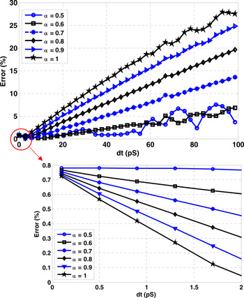
 is equal to one for the Crank–Nicholson scheme (α = 0.5). As previously stated, unconditional stability does not mean that the solution is accurate and physically realistic for any large step size, and the accuracy of the numerical method must also be considered. The maximum percentage error between the proposed method results and the exact solution for the linearly loaded line is shown in Fig. 7.
The spectral radius of the amplification matrix of the proposed FDTD method for different values of α.

The maximum percentage error between the proposed method results and the exact solution for the linearly loaded line versus the time step for different values of α.

It is worth noting that for no incident field illumination, the exact closed-form solution for the time-domain voltage and current on each point of the line, which is shown in Fig. 2, are given by [Reference Paul5]:


wherein:


In the above equations, $\bar{Z}_C$ and γ are the characteristic impedance and the propagation constant of the line, respectively. Since the fully implicit FDTD scheme (α = 1) is an O(Δt 2) perturbation to the Crank–Nicholson method (α = 0.5), resulting in second-order truncation error terms, the accuracy of this approach degrades quickly in the time step above the CFL limit [Reference Crawford and Workman18]. Therefore, as can be observed in Fig. 7, the proposed FDTD method with the smaller weighting factor (α) gives more accurate solutions for large time steps. In other words, in problems that require large time steps to reduce the simulation time, the proposed method with α = 0.5, while ensuring stability, gives lower errors than the other schemes with larger values of α. Moreover, as shown in Fig. 7, when α becomes large for small time steps, the error of the proposed method decreases. It can be concluded that by selecting the optimum value of weighting factor, the proposed FDTD method, in addition to ensuring the stability of the solution for a wide range of time step sizes, presents good accuracy.
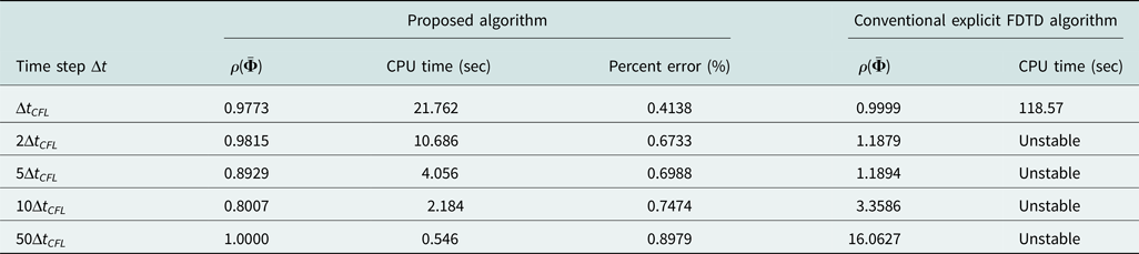
As mentioned in the introduction, in the conventional explicit FDTD method, the time step size must be limited to the CFL number (Δt CFL = Δx/v max) to avoid the instability of the solution. For evaluating the efficiency of the proposed method, the spectral radius of the square matrix $\bar{{\bf \Phi }}$ and computational time of the conventional explicit FDTD approach and the proposed algorithm for different time step sizes are presented in Table 2. As can be observed from this table, the computational time is reduced significantly in the proposed algorithm compared to the conventional explicit FDTD method, while good accuracy is obtained. Furthermore, Table 2 shows that the spectral radius $\rho ( \bar{{\bf \Phi }})$
 in the proposed algorithm is less than or equal to 1 for all time step sizes, while in the conventional explicit FDTD algorithm, the spectral radius $\rho ( \bar{{\bf \Phi }})$
 becomes larger than 1 in time step sizes beyond Δt CFL, i.e., the algorithm becomes unstable.
Comparison of the spectral radius of the square matrix $\bar{{\bf \Phi }}$ and computational time of the conventional explicit FDTD approach and the proposed algorithm.

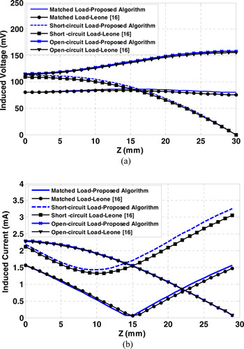
In Fig. 8, the proposed method is used to compute the magnitude of the induced voltage and current distributions on the line endfire illumination ($\theta _E = {-}{\rm \;}\varphi _E = \phi = 90^\circ$ ) with a frequency of 1.3 GHz and an electric-field amplitude of 100 V/m. According to (5) and (6), in the endfire excitation, the incident electric field is polarized in the +y direction, and its amplitude depends only on the x coordinate ($\vec{E}_{inc}( {x, \;t} ) = \vec{a}_yf_W\left({t + \sqrt {\mu \varepsilon } x} \right)$
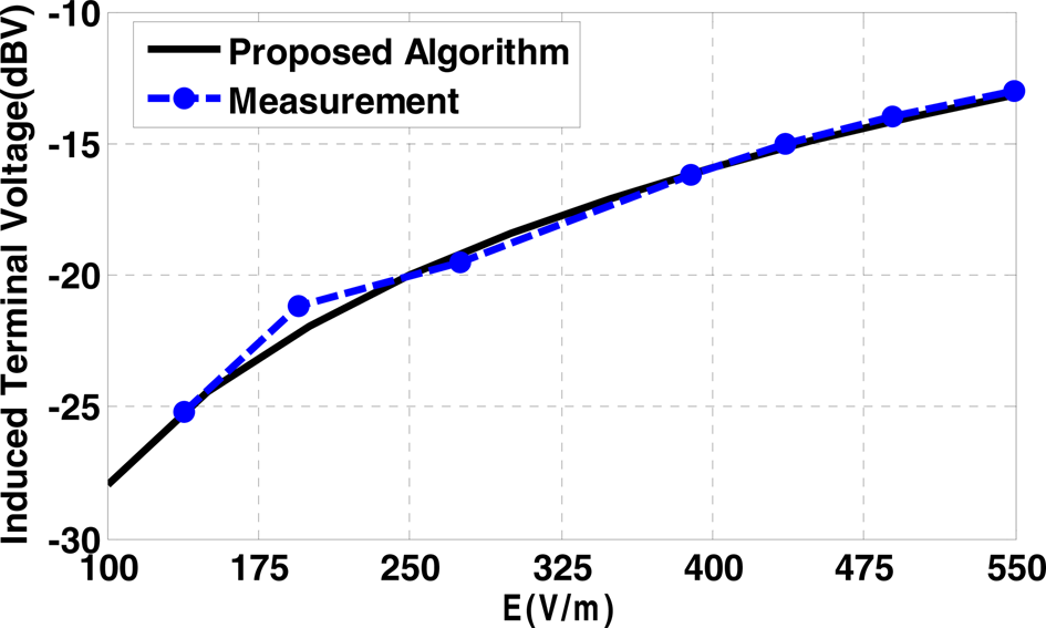
 ). Therefore, since the induced sources due to the incident field (equations (7) and (8)) are symmetric to the center of the line, the magnitude of the induced voltage and current at the line terminals, which are terminated to matched load, will be equal, as shown in Fig. 8. Moreover, as expected, maximum voltage and maximum current are coupled to the line in the open-circuited and short-circuited terminals, respectively. Further, as Fig. 8 shows, the simulated results are in excellent agreement with analytical reference data [Reference Leone and Singer16]. Furthermore, Fig. 9 shows the measured and simulated results for the induced output terminal voltage of the single microstrip line versus the incident electric field amplitude at 1.3 GHz in the case of broadside excitation ($\theta _E = {\rm \;}\phi = 90^\circ , \;{\rm \;}\varphi _E = 0^\circ$
 ). The line is terminated with the matched load. As expected, the increase in the incident EM wave amplitude has led to a rise in the coupled voltage of the TL. Besides, a good agreement between the measured and analytical results is observed in Fig. 9, which confirms the validity of the proposed algorithm.
The magnitude of the induced (a) voltage and (b) current distributions on the single microstrip line for endfire illumination at 1.3 GHz and electric-field amplitude 100 V/m.

Measured and simulated results for the induced output terminal voltage of a single microstrip line versus the incident electric field amplitude for broadside illumination at 1.3 GHz.

Diode power detector excited by uniform EM wave illumination
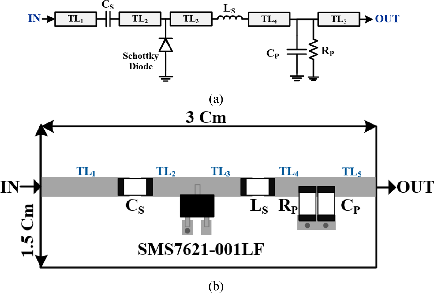
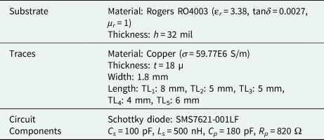
In this subsection, the proposed method is applied to the power detector circuit that generates DC voltage by rectifying the RF/microwave signal through a diode. Furthermore, for verification of the paper method, the designed detector circuit is implemented on a two-layer RO4003 PCB, as shown in Fig. 5(b). The parameters of the circuit are also tabulated in Table 3. The schematic and the PCB layout of the fabricated power detector circuit are also presented in Fig. 10. It should be noted that since the dimensions of the TLs of the detector circuit are much smaller than the wavelength of the incident field at low microwave frequencies, the quasi-TEM assumption of the proposed method is valid.
(a) The schematic diagram and (b) the PCB layout of the fabricated power detector circuit.

Parameters of the fabricated power detector circuit.

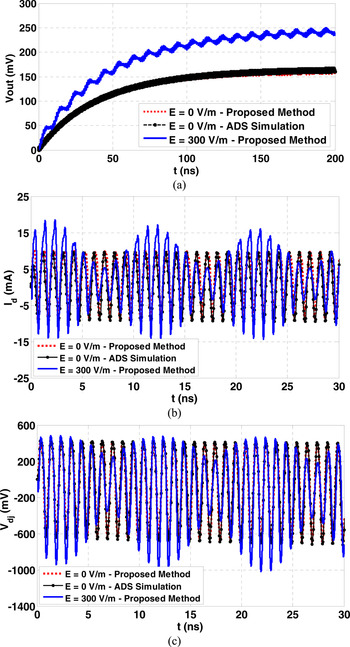
Transient analysis of the detector circuit, which is excited by −1 dBm CW source at 1 GHz, is carried out using the proposed method and ADS Agilent software. Figure 11 shows the time-domain waveforms of the output voltage (V out), diode current (I d), and diode internal junction voltage (V dj) of the circuit, which indicates a good agreement between the two methods. The proposed method results of the detector circuit, which is subjected to 300 V/m incident EM field illumination at 1.1 GHz, are also presented in Fig. 11. In this section, the detector is subjected to endfire illumination by the uniform sinusoidal plane wave. As shown in Fig. 11(a), the incident field coupling to the detector circuit has distorted and increased the output voltage. Further, the mixing of the desired detector input signal and the induced signal due to the nonlinear operation of the diode can be observed in the voltage and current waveforms in Figs 11(b) and 11(c).
Time-domain waveforms of (a) the output voltage, (b) diode current, and (c) diode internal junction voltage of the power detector circuit, which is excited by −1 dBm CW source at 1 GHz as well as the incident plane wave illumination at 1.1 GHz.

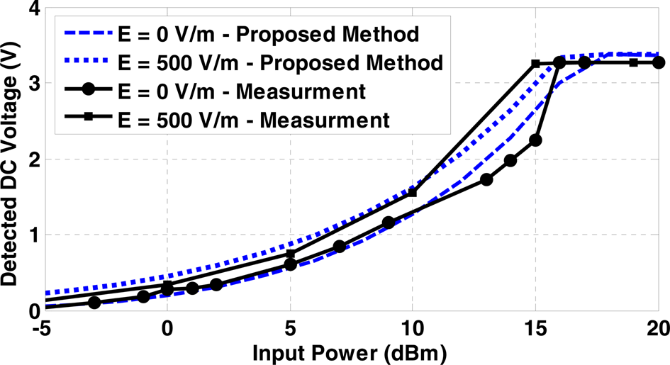
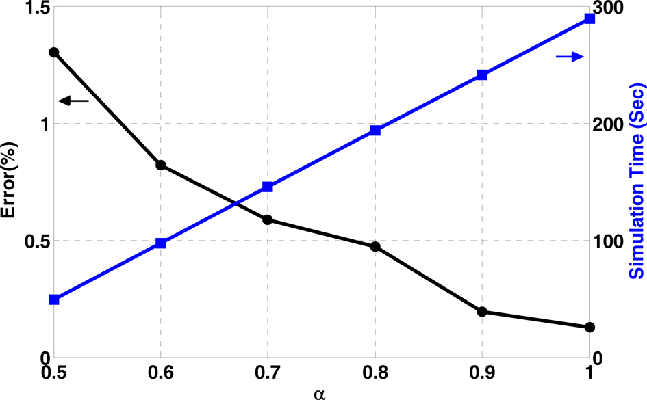
Besides, Fig. 12 shows the measured and proposed method results for the detected DC output voltage versus the input power of the detector circuit subjected to the external uniform plane wave with an amplitude of 500 V/m at 1.1 GHz. The good agreement between the results confirms the accuracy of the proposed method. As can be seen, the high power incident field illumination on the detector circuit has increased the output voltage and also forced the detector to saturate with lower input power. Furthermore, the simulation time and error of the proposed FDTD method for analyzing the diode detector circuit versus the weighting factor parameter (α) are shown in Fig. 13. It is apparent from this figure that good accuracy can be achieved in the shortest possible simulation time by selecting the optimal value for the parameter α in the proposed method.
The measured and proposed method results for the detected DC output voltage versus the input power of the detector circuit, which is excited by the CW source at 1 GHz and the incident plane wave illumination at 1.1 GHz.

The simulation time and error of the proposed FDTD method for analyzing the diode detector circuit versus the parameter α.

Conclusion
The main goal of the current study was to present a new time-domain algorithm for analyzing the nonlinearly loaded TL network excited by the incident EM field. The stability and accuracy of the proposed method have been validated by comparing the analytical and experimental results for two cases, namely a single microstrip line and a Schottky detector circuit. Moreover, it has been shown that the proposed algorithm, while ensuring stability, can reduce simulation time. The accuracy and stability of the proposed method confirm the capability of this method to analyze linear and nonlinear RF/microwave circuits, which are subjected to the external EM wave illumination.
 Zahra Seifi was born in Iran in 1988. She received the B.Sc. and M.Sc. degrees in 2011 and 2013, respectively, in Amirkabir University, Tehran, Iran, where she is currently working toward the Ph.D. degree. Her main areas of research interest are high-frequency signal and noise EM modeling of active devices and circuits, the electromagnetic compatibility problems of electronic systems and ICs, and microwave and mm-wave MMIC circuit design.
 Ayaz Ghorbani received his Postgraduate Diploma, M.Phil., and Ph.D. degrees in Communication Engineering from the University of Bradford, UK, in 1984, 1985, and 1987, respectively. Also, he was on sabbatical leave from 2004 to 2005 at the same university. He has authored or co-authored more than 200 papers in various refereed journals as well as local and international conferences. He also has written (in Persian) more than 10 books in the field of Microwave Engineering, Radar, Electromagnetics and Electromagnetic Compatibility. Dr. Ghorbani received the John Robertshaw Travel Award and the URSI Young Scientists Award from the Bradford University and the General Assembly of URSI, Prague, Czech Republic, in 1987 and1990 respectability. He is currently a Professor in the Department of Electrical and Electronic Engineering, Amirkabir University of Technology, Tehran, Iran. His research areas include microwave components, radio wave propagation, radio link design, electromagnetic compatibility (EMC), and Radar technology.
 Abdolali Abdipour was born in Alashtar, Iran, in 1966. He received his B.Sc. degree in Electrical Engineering from the Tehran University, Tehran, Iran, in 1989, his M.Sc. degree in Electronics from the Limoges University, Limoges, France, in 1992, and his Ph.D. degree in Electronic Engineering from the Paris XI University, Paris, France, in 1996. He is currently a Professor with the Electrical Engineering Department, Amirkabir University of Technology (Tehran Polytechnic), Tehran, Iran. He has authored five books and has authored or co-authored over 300 papers in refereed journals and local and international conferences. His research areas include wireless communication systems (RF technology and transceivers), RF/microwave/millimeter-wave/THz circuit and system design, electromagnetic (EM) modeling of active devices and circuits, high-frequency electronics (signal and noise), nonlinear modeling, and analysis of microwave devices and circuits.