2.1. The cathode electron injection

When an analytical ionisation source is used, new pairs of electrons and ions are generated continuously regardless of existing electrons, thus a quasi-neutral cathode boundary condition can be applied to maintain the neutrality of the plasma in the simulation domain. However, when MCC is used instead, the ionisation is triggered by energetic electrons, such that a cathode is needed to continuously supply electrons like real Hall thrusters. Therefore, we set the plane $x=246$ to be the cathode boundary, shifted by 10 cells from the maximum $x=256$ boundary, which continuously and uniformly injects electrons into the simulation domain. The prescribed cathode electron injection current is chosen to be $I_{\textrm {inj}} \approx 0.3$ A, which is found to be sufficient to sustain MCC ionisation in the present simulations. It should be noted that $I_{\textrm {inj}}$ is a numerical source parameter in the present cathode model and should not be interpreted as a self-consistent discharge current of a real Hall thruster. A realistic discharge current would require a self-consistent cathode–plasma coupling model and an external circuit/current-balance treatment, which are beyond the scope of the present work. The temperature of the injected electrons is 10 eV. To facilitate the entry of cathode-emitted electrons into the channel, an additional drifting velocity along $-x$ is added with 3 times of the corresponding thermal velocity. As we can see, there are a number of free parameters of the cathode boundary that may affect the simulation, which is, however, beyond the scope of this paper, and will be left as a future work to be studied in more detail.

2.2. Neutral gas fluid solver

As our first step of coupling the ionisation using MCC with self-consistent calculation of the neutral gas density, only the continuity equation along the axial direction is considered and solved numerically with a constant axial fluid velocity $u_z$

(2.2) \begin{align} \dfrac {\partial n_a}{\partial t} + u_z \dfrac {\partial n_a}{\partial z} = - S_i(x, y, z), \end{align}

where $n_a$ is the neutral gas density, $S_i$ is the local ionisation rate and the subscript `a’ is used to denote the neutral atom. The present neutral model does not include a surface recycling source. A more complete neutral balance would contain an additional source term associated with ion recombination and neutral re-emission at the wall and anode surfaces. Such a model would require assumptions for the surface recombination probability, re-emitted neutral energy and angular distributions and the near-wall neutral transport. These effects are not included in the present study.

Figure 2.

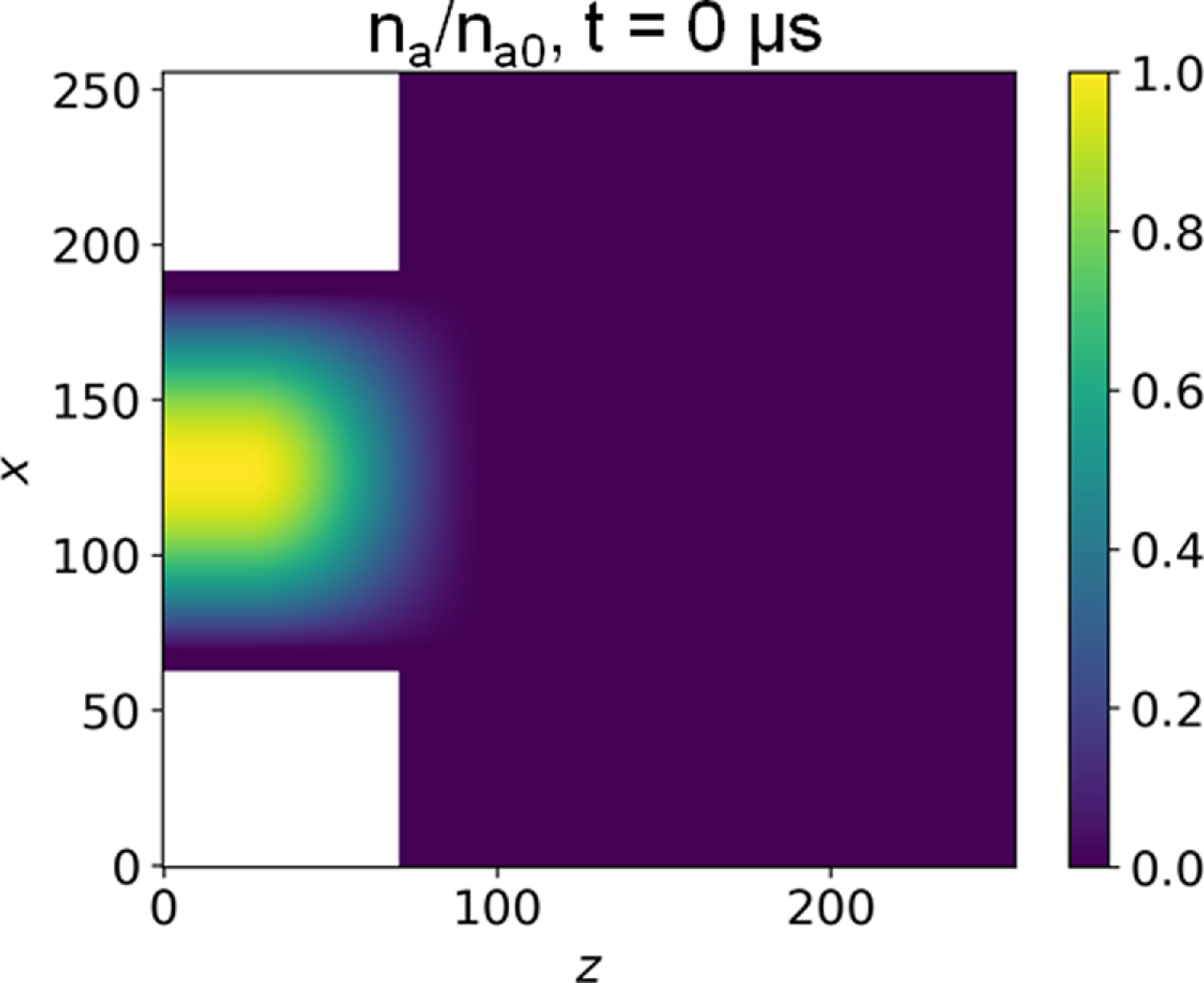
Initial neutral gas density profile. The $z$ and $x$ values represent grid indices.

To set a reasonable initial neutral gas density profile by using ionisation source function, we consider the steady state, where $\partial n_a / \partial t = 0$ , and assume that $S_i$ is uniform in the x and y directions and varies only with z, this allows us to solve the 1-D continuity equation with constant axial velocity to obtain the initial profile. The ionisation source function that is commonly used in the literature (Charoy et al. Reference Charoy2019; Villafana et al. Reference Villafana, Cuenot and Vermorel2023; Xie et al. Reference Xie, Luo, Zhou and Zhao2024) is

(2.3) \begin{align} S_i(z) = S_0 \cos {\left ( \pi \dfrac {z - z_m}{z_2 - z_1} \right )}, \end{align}

if $z\in [z_1,z_2]$ , otherwise zero, $z_m = 0.5(z_1+z_2)$ . Analytically solve the steady-state continuity equation leads to

(2.4) \begin{align} n_a(z) = \dfrac {n_{a0}}{2} \left [ 1 - \sin {\left ( \pi \dfrac {z-z_m}{z_2-z_1} \right )} \right ], \end{align}

for $z\in [z_1,z_2]$ , where $n_{a0}$ is the peak neutral gas density value, for which $n_a(z_1)=n_{a0}$ . For $z \lt z_1$ , we set $n_a(z) = n_{a0}$ , and for $z\gt z_2$ , we set $n_a(z) = 0$ , thus a relation between $n_{a0}$ and $u_z$ can be obtained

(2.5) \begin{align} n_{a0} = \dfrac {2 S_0}{u_z} \dfrac {z_2-z_1}{\pi }. \end{align}

Setting $S_0 = 9.55 \times 10^{23}$ m $^{-3}$ s $^{-1}$ , the commonly used value, and $z_1 = 0.25$ cm, $z_2 = 1$ cm, $n_{a0} = 1.5 \times 10^{19}$ m $^{-3}$ , we obtain $u_z = 304$ m s^–1. However, simulations show that an increasing fluid speed can reduce the ionisation oscillation (or the so-called breathing mode (Choueiri Reference Choueiri2001; Boeuf & Smolyakov Reference Boeuf and Smolyakov2023)) frequency, which is advantageous for faster simulation convergence. We thus apply $u_z = 304 \times 3 = 912$ m s^–1 with $n_{a0} = 1.5 \times 10^{19}$ m $^{-3}$ .

In addition, a radial tapering factor is applied to the initial neutral density profile. Near the channel surfaces, the electron density and ionisation rate are relatively low because of the wall sheath. Neutral atoms in these regions can therefore be weakly ionised and convected downstream along the channel surfaces, which is referred to here as near-wall neutral leakage. To reduce the number of neutral particles initially placed in the near-wall low-ionisation regions and to accelerate the convergence of the simulation, the initialised axial neutral density profile is multiplied by a cosine tapering function in the radial direction. This tapering is applied only to the initial neutral field. During the subsequent simulation, the neutral gas is injected according to the prescribed neutral injection condition, without this radial tapering modifying the imposed neutral supply. Therefore, this treatment is used only to reduce the initial computational burden and is not expected to affect the quasi-steady results after the initial transient. Therefore,

(2.6) \begin{align} n_a(z,x) = &\dfrac {n_{a0}}{2} \Bigg [ 1 - \sin {\left ( \pi \dfrac {z-z_m}{z_2-z_1} \right )} \Bigg ] \cos {\left ( \pi \dfrac {x-x_m}{x_2 - x_1} \right )}, \end{align}

for $x\in [x_1,x_2]$ , otherwise zero. Here, $x_m=1.28$ cm is the centre of the channel, $x_2-x_1 = 1.1008$ cm is equal to 0.86 times the channel width 1.28 cm. Along the azimuthal $y$ direction, $n_a$ is set to be uniform initially. The initial neutral gas density profile in the $z$ – $x$ plane is shown in figure 2.

2.3. Magnetic-field configuration

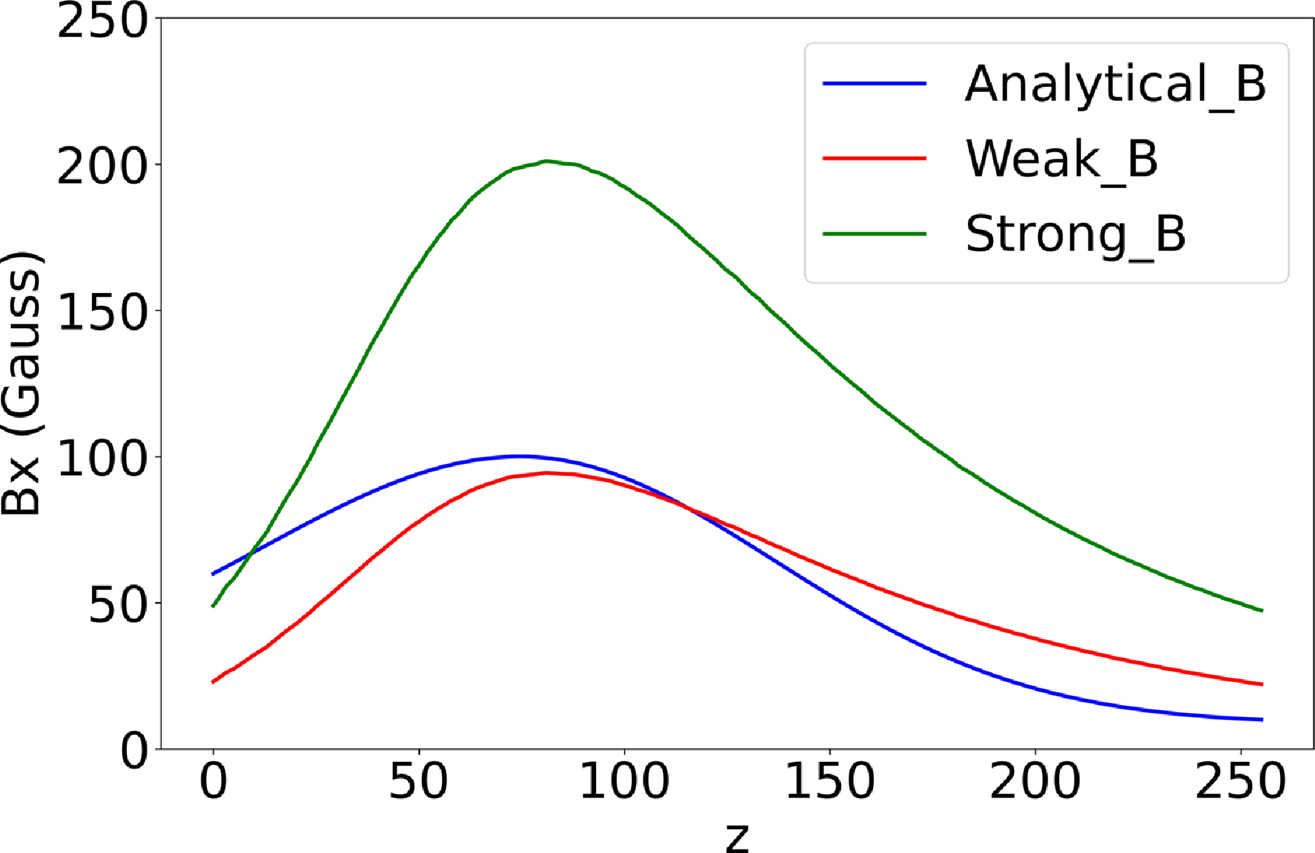
There were three simulation cases labelled analytic-B, strong-B and weak-B studied in the previous paper (Zhong et al. Reference Zhong, Zeng, Zhao and Yu2026). Analytic-B applied the commonly used analytic-B field with only the radial component (Villafana et al. Reference Villafana2021, Reference Villafana, Cuenot and Vermorel2023; Xie et al. Reference Xie, Luo, Zhou and Zhao2024)

(2.7) \begin{align} B_x(z) = a_k \exp {\left [ -\dfrac {(z-z_{B_{max}})^2} {2 \sigma ^2} \right ]} + b_k, \end{align}

where $k=1$ for $z \leqslant z_{B_{max}}$ and $k=2$ for $z\gt z_{B_{max}}$ . With the given parameters, $B_A = B(z=0)=60$ Gauss, $B_C = B(z=2.56\,\text{cm}) = 10$ Gauss, $B_{max} = B(z=z_{B_{max}})=100$ Gauss, $z_{B_{max}} = 0.75$ cm, and $\sigma = 0.625$ cm, $a_k$ and $b_k$ can be calculated according to

(2.8) \begin{align} a_1 &= \dfrac {B_{max} - B_A} {1-\exp {[-z_{B_{max}}^2/(2\sigma ^2)]}} \approx 77.9 \nonumber \\[7pt] a_2 &= \dfrac {B_{max} - B_C} {1-\exp {[-(2.56\,\text{cm}-z_{B_{max}})^2/(2\sigma ^2)]}} \approx 91.4 \end{align}

and $b_1 = B_{max} - a_1$ , $b_2 = B_{max} - a_2$

Figure 3.

Magnetic-field configuration (a) and 1-D magnetic-field strength at three radial positions along $z$ (b) of the weak-B case (the strong-B case differs only in having double the field strength). The $z$ and $x$ values represent grid indices.

Figure 4.

Magnetic-field strength along the centreline for three cases.

Figure 5.

Results of the mean ion number density over time of three cases with different $f_{pn}$ of the strong-B case.

Figure 6.

The ion current at the $z = 256$ plane over time of three cases with different $f_{pn}$ of the strong-B case. The $z$ values represent grid indices. (a) The results calculated by macro-particle data. (b) The results calculated by field data.

Strong-B and weak-B applied a more realistic magnetic-field configuration generated by the FEMM software (www.femm.info); They differ only in magnitude: strong-B has an approximately 200 Gauss peak value on the centreline along $z$ , while weak-B has approximately 100 Gauss, as shown in figure 3; the magnetic-field strength along the centreline for three cases is shown in figure 4. Both the fields were calculated in cylindrical geometry. When using these fields in a Cartesian PIC code, we cannot strictly guarantee $\boldsymbol{\nabla }\boldsymbol{\cdot }\boldsymbol{B} = 0$ in Cartesian coordinates. However, we have evaluated $\boldsymbol{\nabla }\boldsymbol{\cdot }\boldsymbol{B}$ in the channel for both coordinate systems, and the results show little discrepancy between them. Alternatively, the PIC solver itself could be rewritten in cylindrical coordinates, but such an undertaking requires substantial development effort and lies beyond the scope of this study. Consequently, the present work employs a Cartesian PIC framework combined with magnetic fields from FEMM solved in cylindrical coordinates.

2.4. Summary

In this paper, we continue to study these three cases, and load their results at $10^6$ time steps (15 $\unicode{x03BC}$ s) as initialisation with a scaling factor $f_{pn}$ . If $f_{pn}\gt 1$ , each macro-particle loaded will be copied $f_{pn}$ times with the same position and velocity, such that there are more macro-particles at the initialisation, and the particle weight will be reduced by $f_{pn}$ accordingly. The simulation results of the ion number density over time of the strong-B case are shown in figure 5. Although the ion density $n_{i}$ varies significantly over time, the fundamental characteristics of the instability wave – such as its wavelength and frequency – have stabilised, we will show these in § 3.

We have compared the effect of the number of macro-particles for the three strong-B cases with different $f_{pn}$ , the extracted ion currents $f_{pn}$ are provided in figure 6. We employed two methods to calculate the ion current. The first method utilises macro-particle data. Specifically, only macro-particles located in the last grid cell along the $z$ -direction, which are to exit the simulation domain in the next time step, contribute to the current calculation. This method is exact. However, since the $f_{pn} = 3$ case was a test run for which macro-particle data were not saved (only field data were retained) because of the large storage, this first method was applied only to the $f_{pn} = 1$ and $f_{pn} = 10$ cases. The results are shown in figure 6(a). The ion current for the $f_{pn} = 10$ case exhibits significant oscillation, but its mean value (0.0240) is close to that of the $f_{pn} = 1$ case (0.0205).

The second method calculates the ion current using field data by evaluating $ \langle n_i \boldsymbol{\cdot }e \boldsymbol{\cdot }v_{i,z} \rangle \times A$ at the last node along z. Here, $\langle \ldots \rangle$ denotes averaging over the $x$ and $y$ directions, and $A$ is the cross-sectional area of the plume region. The results are shown in figure 6(b). The ion currents for the $f_{pn} = 3$ and $f_{pn} = 10$ cases oscillate significantly. Their mean values are close, being 0.0204, 0.0223 and 0.0241 for the $f_{pn} = 1$ , $f_{pn} = 3$ and $f_{pn} = 10$ cases, respectively.

Additionally, the ion current shown here is the ion flux crossing the downstream ion–current diagnostic plane. It is therefore not equivalent to the total ion production rate or to the ion beam current of a fully calibrated Hall thruster model. Moreover, the present 3-D simulation domain covers only a finite azimuthal segment, $L_y=6.4\,\mathrm{mm}$ , rather than the full annular circumference of a Hall thruster. Thus, the measured ion current should be interpreted as a local-sector diagnostic quantity, not as the full-annulus ion beam current. A full-thruster-equivalent ion current would require additional geometrical scaling and assumptions about azimuthal periodicity or uniformity. In the present simulation, ions may also be lost to the wall, anode, and other absorbing boundaries. Moreover, the prescribed cathode electron injection current is not a self-consistent discharge current. Therefore, the ratio $I_i/I_{\textrm {inj}}$ should not be interpreted as the current utilisation efficiency of a real Hall thruster.

Figure 7.

The electron density averaged over the $x$ and $y$ directions along $z$ , for three cases with different $f_{pn}$ in the strong-B configuration. The $z$ values represent grid indices. All cases correspond to the peak convergence phase shown in figure 5, with simulation times of 22.5 $\unicode{x03BC}$ s for $f_{pn}=1$ , 28.05 $\unicode{x03BC}$ s for $f_{pn}=3$ and 30 $\unicode{x03BC}$ s for $f_{pn}=10$ .

Figure 8.

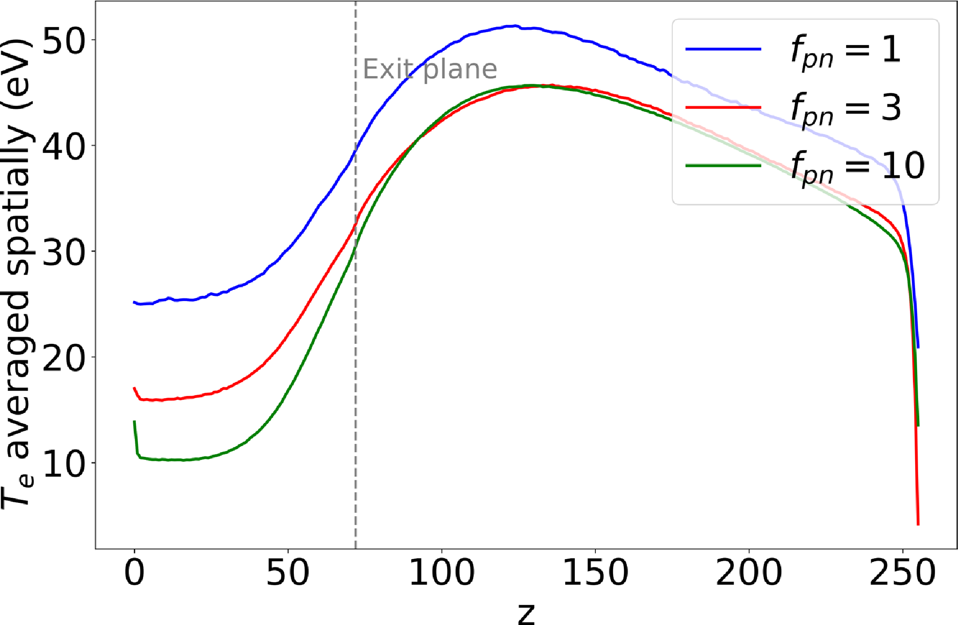
The electron temperature averaged over the $x$ and $y$ directions along $z$ , for three cases with different $f_{pn}$ in the strong-B configuration. The $z$ values represent grid indices. All cases correspond to the peak convergence phase shown in figure 5, with simulation times of 22.5 $\unicode{x03BC}$ s for $f_{pn}=1$ , 28.05 $\unicode{x03BC}$ s for $f_{pn}=3$ and 30 $\unicode{x03BC}$ s for $f_{pn}=10$ .

Figure 9.

Results of the mean ion number density over time of three cases with $f_{pn}=10$ but different B fields. The black solid curve is a reference of the strong-B case with $f_{pn}=1$ .

The electron density averaged over the $x$ and $y$ directions along $z$ is shown for the three cases in figure 7. All cases correspond to the peak convergence phase shown in figure 5, with simulation times of 22.5 $\unicode{x03BC}$ s ( $f_{pn} = 1$ ), 28.05 $\unicode{x03BC}$ s ( $f_{pn} = 3$ ) and 30 $\unicode{x03BC}$ s ( $f_{pn} = 10$ ). It appears that the $f_{pn} = 1$ case shows a significant discrepancy compared with the others.

Table 1.

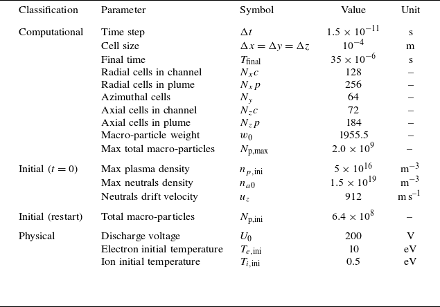
Simulation parameters.

Table 1. Long description

The table presents simulation parameters categorized into computational, initial, and physical conditions. It has 13 rows and 5 columns. The columns are labeled Classification, Parameter, Symbol, Value, and Unit. The computational section includes parameters such as time step, cell size, final time, radial cells in channel, radial cells in plume, azimuthal cells, axial cells in channel, axial cells in plume, macro-particle weight, and max total macro-particles. The initial section at t=0 includes max plasma density, max neutrals density, and neutrals drift velocity. The initial (restart) section includes total macro-particles. The physical section includes discharge voltage, electron initial temperature, and ion initial temperature. Each row lists the parameter, its symbol, value, and unit. For example, the time step is represented by Δt with a value of 1.5 x 10^-11 seconds. The cell size is represented by Δx = Δy = Δz with a value of 10^-4 meters. The final time is represented by T_final with a value of 35 x 10^-6 seconds. The radial cells in channel is represented by N_xc with a value of 128. The radial cells in plume is represented by N_xp with a value of 256. The azimuthal cells is represented by N_y with a value of 64. The axial cells in channel is represented by N_zc with a value of 72. The axial cells in plume is represented by N_zp with a value of 184. The macro-particle weight is represented by w_0 with a value of 1955.5. The max total macro-particles is represented by N_p,max with a value of 2.0 x 10^9. The max plasma density is represented by n_p,ini with a value of 5 x 10^16 m^-3. The max neutrals density is represented by n_a0 with a value of 1.5 x 10^19 m^-3. The neutrals drift velocity is represented by u_z with a value of 912 m/s. The total macro-particles is represented by N_p,ini with a value of 6.4 x 10^8. The discharge voltage is represented by U_0 with a value of 200 V. The electron initial temperature is represented by T_e,ini with a value of 10 eV. The ion initial temperature is represented by T_i,ini with a value of 0.5 eV.

The electron temperature averaged over the $x$ and $y$ directions along $z$ is shown in figure 8. As before, all cases correspond to the peak convergence phase from figure 5. Again, the $f_{pn} = 1$ case shows a notable discrepancy compared with the others.

As can be seen, increasing the number of macro-particles modifies the $n_i$ evolution to some extent, and we chose the most macro-particles that we can apply so far with $f_{pn}=10$ for running the other two cases in order to obtain less noisy results. The $n_i$ evolution of the three cases with $f_{pn}=10$ are shown in figure 9, from which different stages of the ionisation breathing mode can be identified and will be referred to later in the paper. Other parts of the simulation methods, such as the cathode injection, the MCC ionisation and the fluid solver on the continuity equation are the same as the previous paper (Zhao & Zhong Reference Zhao and Zhong2025; Zhong et al. Reference Zhong, Zeng, Zhao and Yu2026). The total computational cost for the strong-B case, from the first restart to the last, was approximately $1.35 \times 10^{5}$ CPU core hours. The simulation ran on a computing node equipped with dual AMD EPYC 9754 CPU, utilising 128 MPI processes, with a step time of approximately 6.5 s per time step at the peak of $n_i$ and approximately 1.0 s per time step at its trough. At last, all the simulation parameters are summarised in table 1. Note that the macro-particles parameters in table 1 are from the strong-B case with $f_{pn}=10$ .

Figure 10.

Azimuthal electric field $E_y$ at the middle plane of $y$ (top row), at the middle plane of $x$ (middle row) and at the plane of $z=70$ (bottom row) of cases strong-B (left), weak-B (middle) and analytic-B (right) at the same oscillating stage of $n_i$ over $t$ .

3.1. Correlation between the electron density and the azimuthal electric field

First, snapshots of $E_y$ in the $z$ – $x$ , $z$ – $y$ and $x$ – $y$ planes are presented for the three cases, each captured at the same convergence time of the ion number density oscillation. These snapshots are shown in figure 10, and the selected times are indicated in the ion-density evolution shown in figure 9. The specific times selected are 24.00 $\unicode{x03BC}$ s for the analytic-B case, 30.00 $\unicode{x03BC}$ s for the strong-B case and 33.00 $\unicode{x03BC}$ s for the weak-B case, as indicated in the ion number density plot (figure 9). Note that the $x$ – $y$ snapshots are taken inside the channel at $z=70$ ; the $z$ – $x$ snapshots are taken at the mid-plane of $y$ ; and the $z$ – $y$ snapshots are taken at the mid-plane of $x$ . Figure 11, figure 12 and figure 13 show snapshots of $E_y$ at different convergence times for the strong-B, weak-B and analytic-B cases, respectively. The observed wave patterns exhibit characteristic wavelengths on the millimetre scale and frequencies in the megahertz range, consistent with the properties of electron cyclotron drift instability, with the pattern being most pronounced in the analytic-B case, less distinct in the strong-B case and barely discernible in the weak-B case.

The correlation terms between the electron density and the azimuthal electric field, i.e. $\langle n_e E_y \rangle$ , averaged spatially along $y$ and temporally within different time periods, are presented in figure 14 for the strong-B case. The first three panels share the same colour bar range, and are averaged around $t_{mean}=16.5$ , 19.5 and 22.5 $\unicode{x03BC}$ s, respectively, within time length $T_{mean} = 3$ $\unicode{x03BC}$ s using data at every 1000 time steps (namely 15 ns). One can find these three corresponding times in figure 9 (the strong-B case line) around the local minimum of $n_i$ , such that the magnitude of $\langle n_e E_y \rangle$ decreases from $5 \times 10^{19}$ V/m $^{4}$ at $t_{mean}=16.5$ $\unicode{x03BC}$ s to a local minimum of approximately $2 \times 10^{19}$ V/m $^{4}$ at $t_{mean}=19.5$ $\unicode{x03BC}$ s and increases back at $t_{mean}=22.5$ $\unicode{x03BC}$ s. Since $\langle n_e E_y \rangle$ reflects the electron transport due to the field oscillations of the instability, these three panels indicate that the major electron transport occurs at the upper region in the radial direction where the magnetic field is relatively low compared with the lower radial region. In the axial direction, the major electron transport due to the instability occurs at the thruster exit and the plume region near the exit.

Figure 11.

Azimuthal electric field $E_y$ at the middle plane of $y$ (top row), at the middle plane of $x$ (middle row) and at the plane of $z=70$ (bottom row) of case strong-B at different oscillating stage of $n_i$ over $t$ .

Figure 12.

Azimuthal electric field $E_y$ at the middle plane of $y$ (top row), at the middle plane of $x$ (middle row) and at the plane of $z=70$ (bottom row) of case weak-B at different oscillating stage of $n_i$ over $t$ .

Figure 13.

Azimuthal electric field $E_y$ at the middle plane of $y$ (top row), at the middle plane of $x$ (middle row) and at the plane of $z=70$ (bottom row) of case analytic-B at different oscillating stage of $n_i$ over $t$ .

Figure 14.

The correlation between the electron density and the azimuthal electric field of the strong-B case evaluated using different time periods.

Figure 15.

The axial ionisation profile of strong-B case at different oscillating stage of $n_i$ over $t$ . The $z$ values represent grid indices.

Then, the other three panels in figure 14 share the same colour bar range, and are averaged around $t_{mean}=26.4$ , 28.5 and 31.5 $\unicode{x03BC}$ s, respectively. These time periods correspond to the peak of $n_i$ as shown in figure 9, thus the magnitude of $\langle n_e E_y \rangle$ increases over time. Moreover, the stronger value of $\langle \delta n_e \delta E_y\rangle$ near the upper radial region can be related to the local magnetic-field asymmetry in the realistic magnetic-field cases. In the present FEMM-based magnetic-field map, the radial magnetic-field component is weaker near the upper channel wall and the outer plume region. For a given local electric field, a weaker magnetic field reduces the electron magnetisation and increases the local azimuthal $E\times B$ drift velocity

(3.1) \begin{align} \boldsymbol{u}_{E\times B} = \frac {\boldsymbol{E}\times \boldsymbol{B}}{B^2}. \end{align}

For a nearly radial magnetic field, this corresponds approximately to $u_{E\times B,y}\sim E_z/B_x$ . Therefore, the lower- $B$ region can provide a stronger local drift drive for the azimuthal EDI. This is consistent with the larger $E_y$ oscillation amplitude observed near the upper radial region. It should also be noted that the turbulent correlation $\langle \delta n_e \delta E_y\rangle$ is not determined by the electric-field amplitude alone. It depends on both the fluctuation amplitudes and the phase correlation between density and electric-field fluctuations. Thus, the enhanced value of $\langle \delta n_e \delta E_y\rangle$ near the upper wall indicates that the large $E_y$ oscillation is accompanied by a non-vanishing density-field correlation.

Comparing the results, it can be seen that not only the magnitude but also the shape of the electron-transport path changes at different stages of the low-frequency ionisation breathing-mode oscillation. Therefore, figure 15 shows the axial ionisation profiles of the strong-B case at different oscillation stages of $n_i$ . These profiles are averaged over the $x$ and $y$ directions and are significantly affected by the breathing-mode oscillation. In the electron momentum conservation equation, the fluctuation correlation $\langle \delta n_e \delta E_y\rangle$ acts as an anomalous momentum-transfer term that influences the electron velocity, thereby affecting the axial electron current density $j_{e,z}$ . So we provide $j_{e,z}$ averaged temporally over different periods and spatially in the $y$ direction for strong-B case in figure 16, the behaviour of $j_{e,z}$ correlates well with the variations in $\langle n_e E_y \rangle$ , $j_{e,z}$ increases as $\langle n_e E_y \rangle$ rises. Concurrently, a path from the top of the plume to the channel gradually forms.

Figure 16.

Value of $j_{e,z}$ ( $z$ , $x$ ) averaged temporally over different periods and spatially in the y-direction for the strong-B case.

Figure 17.

The correlation between the electron density and the azimuthal electric field of the analytic-B case evaluated using different time periods.

Figure 18.

The correlation between the electron density and the azimuthal electric field of the weak-B case evaluated using different time periods.

Next, the corresponding $\langle n_e E_y \rangle$ results of the analytic-B case are shown in figure 17. Again, the considered three times ( $t_{mean}=$ 16.5, 19.425 and 24 $\unicode{x03BC}$ s) correspond to a gradual increase of the $n_i$ as shown in figure 9. Besides the detailed difference of the results at these three times, the overall trends are the same, namely high electron transport due to the instability are expected to occur at the thruster exit and near the surface inside the discharge channel, which is greatly different from that of the strong-B case. This result indicates that the commonly used analytic-B field considering only the radial component should be replaced by more realistic B field to obtain more accurate electron transport.

At last in this subsection, the corresponding $\langle n_e E_y \rangle$ results of the weak-B case are shown in figure 18. Many results at different time steps are presented during the growth of $n_i$ , but overall the electron transport looks very different from the strong-B and the analytic-B case. The results at $t_{mean}=$ 16.5 and 31.5 $\unicode{x03BC}$ s are closer, because at least $n_i$ are not too low, and the EDI could be established and evolve. Nevertheless, as can be seen in figure 9, in between these two times, $n_i$ drops to and maintains at a very low value (approximately $0.4 \times 10^{17}$ m $^{-3}$ ), thus the EDI could not be established, and the plasma behaviour is completely abnormal. Since the weak-B case has only a peak $B$ value of approximately 100 Gauss along the centreline, it could be expected that electrons are not well confined by the magnetic field compared with the other two cases.

3.2. The instability induced turbulent electron mobility

In this subsection, using the $\langle n_e E_y \rangle$ correlation obtained in the simulations, the electron mobility due to the instability can be computed. For clarity, four mobility-related diagnostics are used in this work. The first two, $\mu _{z}^{turb}$ and $\mu _{\perp }^{turb}$ , are correlation-based turbulent mobility estimates derived from the density–electric-field fluctuation correlation. The other two, $\mu _{z,PIC}^{(1)}$ and $\mu _{z,PIC}^{(2)}$ , are direct PIC mobility diagnostics obtained from the simulated axial electron velocity and axial electric field. Their definitions are given below when they are first used. As derived by Lafleur et al. (Reference Lafleur, Baalrud and Chabert2016a), the fluctuation-correlation term contributes to the electron mobility as (Zhao & Zhong Reference Zhao and Zhong2025)

(3.2) \begin{align} \mu _{z}^{turb} \equiv - \dfrac {\langle n_e E_y \rangle }{B_x n_e E_z}, \end{align}

ignoring the classical transport due to electron–neutral collisions. Note that $\mu _{z}^{turb}$ is defined as negative for electron transport to the anode in this paper. During the computation, since the averaged electron density and the axial electric field are used, they are plotted alongside with $\mu _{z}^{turb}$ at typical times for the strong-B case in figure 19, the analytic-B case in figure 20 and the weak-B case in figure 21.

Figure 19.

The electron mobility $\mu _{z}^{turb}$ , averaged electron density, averaged axial electric field of the strong-B case evaluated using different time periods.

Figure 20.

The electron mobility $\mu _{z}^{turb}$ , averaged electron density, averaged axial electric field of the analytic-B case evaluated using different time periods.

For the strong-B case shown in figure 19, two representative times are selected, namely 16.5 and 31.5 $\unicode{x03BC}$ s. By comparing $\mu _{z}^{turb}$ with the corresponding $\langle n_e E_y\rangle$ profiles shown in figure 14, it can be seen that regions with larger $\langle n_e E_y\rangle$ generally correspond to larger values of $\mu _{z}^{turb}$ , as expected from the definition of the correlation-based turbulent mobility. The corresponding turbulent mobility is enhanced because the fluctuation-correlation numerator is larger and because the local magnetic field entering the cross-field transport estimate is weaker. An exception is the dividing line between negative and positive $\mu _{z}^{turb}$ in the upper radial region. As will be shown below, this sign-changing structure can be removed when the mobility is evaluated in the direction perpendicular to the local magnetic-field lines. Nevertheless, we first present $\mu _{z}^{turb}$ , which is defined with respect to the axial $z$ direction, in order to show how the axial mobility estimate is affected by the realistic magnetic-field configuration. In addition, comparing the axial electric-field profiles at the two selected times in figure 19 shows that the strength of $E_z$ near the exit decreases at 31.5 $\unicode{x03BC}$ s, when $n_i$ is close to its peak value, compared with that at 16.5 $\unicode{x03BC}$ s.

Next, looking at the $\mu _{z}^{turb}$ of the analytic-B case in figure 20, $t_{mean}=16.5$ and 24 $\unicode{x03BC}$ s are chosen, the corresponding $\langle n_e E_y \rangle$ plots are presented in figure 17. It can be seen that near the surface inside the discharge channel, relatively large $\mu _{z}^{turb}$ is expected, but the high values of $\langle n_e E_y \rangle$ in the centre at the thruster exit lead to reduced extent of $\mu _{z}^{turb}$ , due to the combined effects of $n_e$ , $E_y$ and $B_x$ .

The $\mu _{z}^{turb}$ of the weak-B case is shown in figure 21. Again, higher values of $\langle n_e E_y \rangle$ (shown in figure 18) lead to stronger electron mobility to the anode. Because the magnetic field is not strong enough in this case, the peak electron density moves from the region inside the channel at 16.5 $\unicode{x03BC}$ s to the region outside of the channel at 31.5 $\unicode{x03BC}$ s. The axial electric field cannot be established near the thruster exit, but rather moves to the downstream region, indicating an abnormal Hall thruster discharge.

In addition, because (3.2) was derived originally based on the purely radial magnetic-field assumption, but in the strong-B and the weak-B cases, the magnetic field contains both radial and axial components. It would be more reasonable to analyse the electron mobility perpendicular to the $B$ field, i.e.

(3.3) \begin{align} \mu _{\perp }^{turb} \equiv - \dfrac {\langle n_e E_y \rangle }{B n_e E_\perp }, \end{align}

where $B=(B_x^2 + B_z^2)^{1/2}$ , and $E_\perp$ can be evaluated by transforming $\boldsymbol{E}=(E_\parallel ,E_\perp )$ into a new coordinate system defined by the two axes that are parallel and perpendicular to the local $\boldsymbol{B}$

(3.4) \begin{align} E_\perp = \dfrac {B_z E_x - B_x E_z}{B}. \end{align}

The perpendicular electron mobility for the strong-B case is plotted in figures 22 and 23 As can be seen, compared with the normal $\mu _{z}^{turb}$ plot of the strong-B case in figure 19, the dividing line between negative and positive $\mu _{z}^{turb}$ in the upper radial region becomes less pronounced under the diagnosis of perpendicular electron mobility. Thus, $\mu _{\perp }^{turb}$ would be a better choice for future analyses of the electron mobility when the magnetic field contains both radial and axial components.

Figure 21.

The electron mobility $\mu _{z}^{turb}$ , averaged electron density, averaged axial electric field of the weak-B case evaluated using different time periods.

Figure 21. Long description

The image contains six panels, each depicting different aspects of the weak-B case evaluated using different time periods. Panel A, Panel B, and Panel C are in the top row, while Panel D, Panel E, and Panel F are in the bottom row. Each panel is a heatmap with contour lines overlaid. The x-axis represents the z-coordinate ranging from 0 to 250, and the y-axis represents the x-coordinate ranging from 0 to 250. Panel A and Panel D show the electron mobility with a color scale ranging from -4 to 4. Panel B and Panel E display the averaged electron density with a color scale ranging from 0 to 1e17 for Panel B and 0 to 1e18 for Panel E. Panel C and Panel F illustrate the averaged axial electric field with a color scale ranging from -4 to 4. Each panel includes annotations for the mean time (t_mean) and the mean temperature (T_mean). The contour lines in each panel represent the flow or field lines. The top row of panels corresponds to a time period of 1199000, while the bottom row corresponds to a time period of 2199000. The heatmaps show variations in electron mobility, electron density, and electric field across the spatial coordinates, with distinct patterns and gradients visible in each panel.

Figure 22.

The perpendicular electron mobility $\mu _{\perp }^{turb}$ and the averaged perpendicular electric field of the strong-B case evaluated using different time periods.

Figure 23.

Perpendicular turbulent electron mobility $\mu _{\perp }^{turb}$ for the strong-B case evaluated over additional time periods. A wider common colour scale is used for all panels to facilitate comparison of the temporal variation during the breathing-mode cycle.

3.3. Direct PIC electron mobility

The electron mobility in the PIC simulations can also be evaluated directly from the simulated axial electron velocity and electric field. Here, two direct PIC mobility diagnostics are considered. The first is

(3.5) \begin{align} \mu _{z,PIC}^{(1)} = \Big\langle \dfrac {u_{ez}}{E_z} \Big\rangle , \end{align}

where $u_{ez}$ denotes the axial electron velocity, $E_z$ denotes the axial electric field and $\langle \ldots \rangle$ denotes the averaged temporally and spatially over $y$ direction. Because it is found that the noise is large, longer periods are used to obtain averaged results over time. The results of the three cases with labelled averaging periods $T_{\textrm {mean}}$ are shown in figure 24.

The $\mu _{z,PIC}^{(1)}$ of the analytic-B case can be compared with $\mu _{z}^{turb}$ shown in figure 20. Although $\mu _{z,PIC}^{(1)}$ is noisy, more negative blue points inside the channel near the surfaces and in the plume near the exit indicate the same trend and shape that can be seen in $\mu _{z,PIC}^{(1)}$ as well, which is circled by the dashed yellow line in figure 24. Similarly, the middle plot of $\mu _{z,PIC}^{(1)}$ of the strong-B case can be compared with $\mu _{z}^{turb}$ shown in figure 19. Again, similar trends can be seen, indicating that $\mu _{z,PIC}^{(1)}$ agrees with $\mu _{z}^{turb}$ . At last, $\mu _{z,PIC}^{(1)}$ of the weak-B case can be compared with $\mu _{z}^{turb}$ shown in figure 21. Negative electron-transport regions can be identified in the downstream plume region, which agrees with $\mu _{z}^{turb}$ .

Figure 24.

The direct PIC mobility diagnostic $\mu _{z,PIC}^{(1)}$ (3.5), computed as the temporal and azimuthal average of the local ratio $u_{e,z}/E_z$ , for the cases analytic-B (left), strong-B (middle) and weak-B (right).

Figure 25.

The electron mobility for the strong-B case. (a) The result $\mu _{z}^{turb}$ calculated by (3.2). (b) The result $\mu _{z,PIC}^{(2)}$ calculated by (3.6).

The second way is

(3.6) \begin{align} \mu _{z,PIC}^{(2)} = \dfrac {\langle u_{ez} \rangle }{\langle E_z \rangle } , \end{align}

This definition yields much less noise. The result for the strong-B case is shown in figure 25. Although the spatial distribution of the mobility obtained from the second way corresponds well to the result calculated by $\langle n_e E_y \rangle$ in the top of the plume region, their magnitudes differ by approximately two orders. This discrepancy is likely because the second method neglects the temporal phase difference between $u_{e,z}$ and $E_z$ .

3.4. The inverse Hall parameter

At last, motivated by Roberts and Jorns (Reference Roberts and Jorns2024), the inverse Hall parameter is plotted for the strong-B case. The mean azimuthal ( $u_{ey}$ ) and axial ( $u_{ez}$ ) electron velocity profiles over $z$ along the centreline or near the surface of the upper radial region (10 cells away from the surface) are given in figure 26(a). These velocities are averaged over the azimuthal space and time period of 12.3 $\unicode{x03BC}$ s as the same as that in figure 24 of the strong-B case. As we can see $u_{ey}$ increases until near the maximum B field, then drops; $u_{ez}$ increases to zero between $z/L =1$ and 2, where $L=L_{zc}=0.72$ cm is the channel length. When computing the inverse Hall parameter $\varOmega ^{-1}=-u_{ez}/u_{ey}$ , only the ranges with $u_{ez}\lt 0$ are considered, such that $\varOmega ^{-1}\gt 0$ . The two $\varOmega ^{-1}\gt 0$ curves on the centreline and near the channel surface are plotted in figure 26(b). Because the magnetic-field configuration, the maximum B field location compared with the channel exit, and many other parameters are all different from those applied in Roberts & Jorns (Reference Roberts and Jorns2024), no agreement is expected, but reasonable magnitudes of $\varOmega ^{-1}$ are achieved. In addition, it is shown that the axial distribution of $\varOmega ^{-1}$ can vary significantly across different radial regions, particularly when considering the perspective of distinct electron-transport paths in various radial zones as identified in this study.

Figure 26.

(a) Mean azimuthal ( $u_{ey}$ ) and axial ( $u_{ez}$ ) electron velocity profiles over $z$ along the centreline labelled `c’ or near the surface of the upper radial region labelled by `s’. (b) The computed inverse Hall parameter over $z$ . Here, $L=0.72$ cm denotes the channel length, and the maximum B field on the centreline at approximately 0.86 cm is indicated using black dashed lines.