1. Introduction
The dispersion phenomenon of mass and heat transport in oscillatory flows has a wide range of applications, from environmental flows in estuaries (Holley, Harleman & Fischer Reference Holley, Harleman and Fischer1970; Fischer Reference Fischer1972), wetlands (Zeng et al. Reference Zeng, Chen, Wu, Li, Wu and Ji2012; Guan et al. Reference Guan, Zeng, Li, Guo, Wu and Wang2021) and oceans (Yasuda Reference Yasuda1984; Zeng et al. Reference Zeng, Yang, Wang, Jiang, Guan, Zhao and Wu2025b ), to pulsating flows in physiological systems (Grotberg, Sheth & Mockros Reference Grotberg, Sheth and Mockros1990; Jiang & Grotberg Reference Jiang and Grotberg1993; Grotberg & Jensen Reference Grotberg and Jensen2004; Lawrence et al. Reference Lawrence, Coenen, Sánchez, Pawlak, Martínez-Bazán, Haughton and Lasheras2019), to oscillating driving flows in microfluidic systems (Morris Reference Morris2001; Vedel, Olesen & Bruus Reference Vedel, Olesen and Bruus2010; Ding Reference Ding2023), etc. The time-dependent velocity field introduces additional complexity compared with the case with a steady flow. Understanding the interplay between diffusion and temporal advection is crucial for predicting and controlling transport processes in various applications. Taylor dispersion theory (Taylor Reference Taylor1953) provides a fundamental analytical tool for characterising the overall transport processes.
The study of the long-time asymptotic dispersion regime for time-dependent flows can date back to the 1960s. Aris (Reference Aris1960) initiated the first analytical investigation of Taylor dispersion in an oscillatory tube flow. He used the classical method of concentration moments proposed by himself (Aris Reference Aris1956) to derive the expression of Taylor coefficient and revealed the fundamental effect of the flow pulsation. The key to the long-time asymptotic solution is the derivation of the purely periodic part of the first-order moment. The development of the moment method was promoted by Brenner & Edwards (Reference Brenner and Edwards1993), who proposed the generalised Taylor dispersion theory that can be applied to not only time-dependent flows but also to extensions with unsteady components in transport flux. Alternative methods include using the special solution of concentration distribution to directly derive Taylor dispersivity for oscillatory flows, e.g. a linearly longitudinal distribution (although not physically sound for infinitely long channels) (Bowden Reference Bowden1965; Chatwin Reference Chatwin1975; Watson Reference Watson1983; Pedley & Kamm Reference Pedley and Kamm1988; Mederos et al. Reference Mederos, Arcos, Bautista and Méndez2020) and Gaussian distribution for unbounded linear shear flow (Smith Reference Smith1982b ; Young, Rhines & Garrett Reference Young, Rhines and Garrett1982). Nevertheless, crucial experimental verification has been undertaken by many researchers (Joshi et al. Reference Joshi, Kamm, Drazen and Slutsky1983; Jensen et al. Reference Jensen, Rio, Hansen, Clanet and Bohr2009; Song & Law Reference Song and Law2015; Nissan, Dror & Berkowitz Reference Nissan, Dror and Berkowitz2017), and more recently by Ding et al. (Reference Ding, Hunt, McLaughlin and Woodie2021) and Elhanati, Dror & Berkowitz (Reference Elhanati, Dror and Berkowitz2023).
Another classical method, the multiscale expansion technique, has also been applied to analyse the long-time asymptotic dispersion coefficient of solute transport in oscillatory flows. Fife & Nicholes (Reference Fife and Nicholes1975) first introduced a two-time-scale general asymptotic solution form of concentration distribution for dispersion problems, which can also treat a time-dependent velocity field. Pavliotis (Reference Pavliotis2002) used the typical two-scale homogenisation method (Pavliotis & Stuart Reference Pavliotis and Stuart2008) to derive the Taylor dispersion coefficient for periodic flows. Ng (Reference Ng2004, Reference Ng2006) applied the multiple-time-scale homogenisation method (Mei et al. Reference Mei, Auriault, Ng, Hutchinson and Theodore1996) proposed by Mei (Reference Mei1992) to study the cases of time-periodic channel flows and tube flows with reversible solute adsorption at the walls. The principles behind these multiscale methods are analogous, although with differences in the specific expansion forms and the selection of scales (Camassa, Lin & McLaughlin Reference Camassa, Lin and McLaughlin2010; Wu & Chen Reference Wu and Chen2014; Ding et al. Reference Ding, Hunt, McLaughlin and Woodie2021). Recent progress and applications have focused on complex oscillatory transport problems (Barik & Dalal Reference Barik and Dalal2019; Chu et al. Reference Chu, Garoff, Przybycien, Tilton and Khair2019; Ding et al. Reference Ding, Hunt, McLaughlin and Woodie2021; Karmakar, Barik & Raja Sekhar Reference Karmakar, Barik and Raja Sekhar2023; Poddar et al. Reference Poddar, Saha, Mondal, Dhar and Mazumder2024).
Recently, the transient dispersion process in time-dependent flows has attracted more interest than the exhaustively explored long-time asymptotic dispersion regime does (Vedel & Bruus Reference Vedel and Bruus2012). The main focus is the complicated temporal evolution of the Taylor–Aris dispersion coefficient. Thus, the method of concentration moments is probably the remaining viable option for analytical studies. We remark that although the Taylor–Gill generalised dispersion model (Gill & Sankarasubramanian Reference Gill and Sankarasubramanian1971) has also been employed by many studies for various oscillatory flows (Gaver & Grotberg Reference Gaver and Grotberg1990; Hazra, Gupta & Niyogi Reference Hazra, Gupta and Niyogi1996; Rana & Murthy Reference Rana and Murthy2016; Wang & Chen Reference Wang and Chen2017b ; Singh & Murthy Reference Singh and Murthy2023), this method can be considered as a kind of cumulant (alternative to moments) expansion technique (Frankel & Brenner Reference Frankel and Brenner1991; Jiang & Chen Reference Jiang and Chen2018). Indeed, the coefficients in Gill’s model can be expressed in moments. Consequently, we will focus on the concentration moment method.
The method of concentration moments is well developed for transport problems with steady flows. Barton (Reference Barton1983) has derived the general expressions for the full transient solution of moments up to the third order (Aquino Reference Aquino2024), using the method of separation of variables (based on the solution by Aris Reference Aris1956). However, for unsteady flows, these results cannot be applied directly. In fact, the time-dependent velocity makes the solution procedure of moments much more cumbersome. In the ordinary differential equations of the expansion coefficients obtained by separation of variables, the coefficient matrix is time-dependent (i.e. the system is non-autonomous) and thus it can considerably increase the complication of the procedure.
Nevertheless, many researchers have aimed to solve the complete concentration moments in time-periodic flows. Yasuda (Reference Yasuda1982, Reference Yasuda1984) used the method of Green’s function to derive the explicit analytical expressions of moments up to the second order for oscillatory currents. Smith (Reference Smith1983) obtained the statistics of concentration moments by a Hermite-series representation of concentration distribution. Dentz & Carrera (Reference Dentz and Carrera2003, Reference Dentz and Carrera2005) developed the approximate solutions of the drift and dispersivity for temporally fluctuating flows, using the Fourier transform and perturbative analysis framework by Attinger et al. (Reference Attinger, Dentz, Kinzelbach and Kinzelbach1999). Mukherjee & Mazumder (Reference Mukherjee and Mazumder1988) introduced a so-called time-dependent ‘eigenvalue’ problem to extend the approach of Barton (Reference Barton1983) to oscillatory flows, using tube and channel flows as examples. The ‘eigenvalue’ problem is in fact in the same form as the cell problem (i.e. the long-time asymptotic local transport problem) derived in the homogenisation method. In addition, this form of time-dependent eigenvalue problem was proposed by Shapiro & Brenner (Reference Shapiro and Brenner1990) based on Brenner’s generalised dispersion theory, despite the lack of intuitiveness. They pointed out that the eigenvalues could be complex numbers and the eigenfunctions were time-periodic (Shapiro & Brenner Reference Shapiro and Brenner1987). Only the zeroth-order moment was discussed for its complete time-dependent solution form, while the higher-order moments were sought in their long-time asymptotic form. Actually, if one imposes a new time variable for the oscillatory velocity field, the physical interpretation and the solution structure of the ‘eigenvalue’ problem will be fundamentally clear. This is the primary aim of our work.
More recently, the method of concentration moments has been extended and applied to the study of transient dispersion in complex oscillatory flows. Vedel & Bruus (Reference Vedel and Bruus2012) extended earlier studies on single-frequency harmonic pulsatile flows (e.g. the work of Mukherjee & Mazumder Reference Mukherjee and Mazumder1988) to encompass the case of multiple-frequency flows (but with the same base frequency). A trial expansion form has been constructed to seek the full solution of the first-order concentration moment. Later, they studied the transient dispersion with a point-source release (Vedel, Hovad & Bruus Reference Vedel, Hovad and Bruus2014). For environmental dispersion in tidal wetland flows, Zeng et al. (Reference Zeng, Chen, Wu, Li, Wu and Ji2012) applied the integral transformation technique to derive the explicit expression for the time-dependent dispersion coefficient, inspiring many subsequent studies (Wu et al. Reference Wu, Zeng, Chen, Li, Shao, Wang and Jiang2012; Wang & Chen Reference Wang and Chen2015; Das et al. Reference Das, Dhar, Kairi, Mondal and Poddar2024a ). A later comprehensive study by Ding et al. (Reference Ding, Hunt, McLaughlin and Woodie2021) revisited the transport problem in wall-driven flows (Stokes layer) (Bandyopadhyay & Mazumder Reference Bandyopadhyay and Mazumder1999; Paul & Mazumder Reference Paul and Mazumder2008). They solved the moment equations up to the third order using series expansions. The analytical results agreed well with their numerical simulations and experimental data.
Apart from the dispersion coefficient, Ding et al. (Reference Ding, Hunt, McLaughlin and Woodie2021) have made the first analytical attempt (to the best of our knowledge) to investigate the temporal evolution of skewness, a fundamental higher-order statistic that reflects the asymmetry of concentration distribution (Chatwin Reference Chatwin1970; Aminian et al. Reference Aminian, Bernardi, Camassa and McLaughlin2015, Reference Aminian, Bernardi, Camassa, Harris and McLaughlin2016). They also analysed the long-time asymptotic behaviour of skewness: the decay rate for a single-frequency flow is
 $t^{-3/2}$
, instead of
 $t^{-1/2}$
for the steady case (Ding et al. Reference Ding, Hunt, McLaughlin and Woodie2021, (28)). This observation is in agreement with the asymptotic analysis by Smith (Reference Smith1982a
, Reference Smith1983).
Although the general solution expression of skewness has been provided by Ding et al. (Reference Ding, Hunt, McLaughlin and Woodie2021) for arbitrary time-dependent flows, the derivation was based on a specific initial condition, i.e. an instantaneous and uniform source release over the cross-section, such that the zeroth-order concentration moment is
 $1$
and the solution procedure can be greatly simplified. Thus, there remains a fundamental need to tackle general initial conditions, particularly for the case with a point-source release. The corresponding solution can then serve as a Green function (Shapiro & Brenner Reference Shapiro and Brenner1990) for arbitrary release scenarios. Vedel et al. (Reference Vedel, Hovad and Bruus2014) have investigated the effect of point-source position on the dispersion coefficient. However, its effect on the higher-order statistics including skewness has not been analytically studied for oscillatory flows.
Kurtosis, another useful higher-order statistic to characterise the deviation of concentration distribution from Gaussian distribution, was not addressed by Ding et al. (Reference Ding, Hunt, McLaughlin and Woodie2021), probably due to the complication introduced by the oscillatory nature of the velocity field. The long-time asymptotic behaviour of kurtosis has been discussed by Smith (Reference Smith1983), concluding that the decay rate for oscillatory flows is
 $t^{-1}$
, the same as that for steady flows (Chatwin Reference Chatwin1972). Although for the steady flows, many researchers have analytically investigated the transient evolution of kurtosis (Andersson & Berglin Reference Andersson and Berglin1981; Aminian et al. Reference Aminian, Bernardi, Camassa and McLaughlin2015; Wang & Chen Reference Wang and Chen2017a
; Guo et al. Reference Guo, Jiang, Chen, Li, Alharbi and Wakeel2022), little analytical work has been done for time-periodic flows. Previous studies had to resort to numerical methods to calculate the high-order moments for kurtosis (Allen Reference Allen1982; Mazumder & Das Reference Mazumder and Das1992; Debnath et al. Reference Debnath, Saha, Mazumder and Roy2019). For example, recent studies by Dhar et al. (Reference Dhar, Das, Poddar and Mondal2022) and Das et al. (Reference Das, Mondal, Poddar and Wang2024b
) have applied the finite-difference method to numerically solve the governing equations of moments up to the fourth order.
Recently, Singh & Murthy (Reference Singh and Murthy2023) and Pal, Singh & Murthy (Reference Pal, Singh and Murthy2025) have derived an integral-form expression of kurtosis. Their comprehensive and systematic studies have applied the method of concentration moments to investigate the transport problem in pulsating non-Newtonian fluid flows. They found that the kurtosis of the case with oscillatory flows, similar to skewness, can also be much smaller than that of steady flows, implicating that the concentration distribution may become Gaussian faster for the oscillatory flows than for steady flows (Mazumder & Das Reference Mazumder and Das1992).
Although the integral-form expression of kurtosis has been obtained, it should be noted that the solution expression is inexplicit: it contains a lot of unsolved nested symbolic integrals with respect to time. This can be seen in (D5)–(D8) in the work of Singh & Murthy (Reference Singh and Murthy2023), where four forms of integrals were defined hierarchically. Analytically solving these nested integrals up to the last-order is a challenging task. In fact, they numerically calculated the integration of these integrals, using Simpson’s 1/3 rule. This numerical solution procedure was previously used by Rana & Murthy (Reference Rana and Murthy2016). As a comparison, the solution expression of the third-order concentration moment by Ding et al. (Reference Ding, Hunt, McLaughlin and Woodie2021) is fully explicit with respect to the time variable (i.e. no unsolved symbolic integrals). Thus, there remains a need to explicitly solve the fourth-order moment for kurtosis.
This study aims to address the issue of the complication induced by the time-periodic velocity field during the analytical solution procedure of concentration moments, especially when solving for higher-order statistics such as skewness and kurtosis. We introduce a new auxiliary time variable for the oscillatory velocity field and extend the original transport problem to a two-time-variable problem (which is analogous to the multi-time scale method). To some extent, the new time dimension can be virtually viewed as an additional ‘transverse’ periodic space. This treatment can not only offer an intuitive physical perspective on the effects of velocity field oscillation on dispersion, but also clarify the structure of the governing equations of moments. More importantly, under this new two-time-variable transport problem, there is no need to re-solve the moment equation. The general solution expressions obtained by Barton (Reference Barton1983) for steady flows can be directly applied to the case of oscillatory flows, because the flow velocity becomes ‘steady’ after ‘splitting’ the time variable. The remaining procedure simply involves: (i) identifying the new eigenvalue problem and (ii) substituting the eigenvalues and eigenfunctions into Barton’s expressions. Therefore, the complications encountered in previous methods can be avoided. It is feasible to analytically investigate the temporal evolution of higher-order statistics for time-periodic flows, analogous to the steady-flow case.
2. Formulation of transport problem and concentration moments
2.1. Governing equation
To illustrate the analytical solution procedure, we consider mass transport in a parallel channel with a time-dependent velocity field. For simplicity, we focus on the two-dimensional transport problem. A typical case is shown in figure 1.
Sketch of solute transport problem in an oscillatory flow created by the oscillating channel wall. Several simulated particle trajectories are shown. The time variable in the oscillatory velocity field can be virtually viewed as an additional ‘transverse’ spatial variable.

The dimensionless form of the whole transport problem can be adopted as follows:
 \begin{align} \frac {\partial C}{\partial t} + u (y, t) \frac {\partial C}{\partial x} & = \frac {1}{\textit{Pe}^2} \frac {\partial ^2 C}{\partial x^2} + \frac {\partial ^2 C}{\partial y^2}, \end{align}
 \begin{align} \left . \frac {\partial C}{\partial y} \right |_{y = 0} &= \left . \frac {\partial C}{\partial y} \right |_{y = 1} = 0, \end{align}
 \begin{align} C | _{t = 0} &= C_{{{ini}}} (y) \delta (x) . \end{align}
The range of the dimensionless variables is
 $- \infty \lt x \lt + \infty$
(the channel length is infinite),
 $0 \lt y \lt 1$
(the dimensionless channel width is
 $1$
) and
 $t \gt 0$
(the time). Note that the following dimensionless parameters and variables have been chosen (the superscript asterisk denotes dimensional variables and parameters):
 \begin{align} x &= \frac {1}{\textit{Pe}} \frac {x^{\ast }}{L^{\ast }}, \quad y =\frac {y^{\ast }}{L^{\ast }}, \quad t = \frac {t^{\ast }}{{L^{\ast }}^2 /D^{\ast }}, \nonumber \\ u &= \frac {u^{\ast }}{U^{\ast }_{\textrm{c}}}, \quad C = \textit{Pe} \frac {C^{\ast }}{C^{\ast }_{{\text{c}}}}, \quad \textit{Pe} = \frac {U^{\ast }_{\textrm{c}} L^{\ast }}{D^{\ast }}, \quad \omega = \frac {\omega ^{\ast }}{D^{\ast } / {L^{\ast }}^2}, \end{align}
where
 $L^{\ast }$
is the channel width,
 $D^{\ast }$
is the solute diffusion coefficient,
 $U^{\ast }_{{\text{c}}}$
is a characteristic velocity and
 $\textit{Pe}$
is the corresponding Péclet number. Here,
 $C^{\ast }_{{\text{c}}}$
is a characteristic concentration constant such that the dimensionless concentration distribution satisfies
 \begin{equation} \int ^{\infty }_{- \infty } \int ^{1}_0 C (x, y, t) \, \textrm{d} y \,\textrm{d} x = 1. \end{equation}
Namely,
 $C$
is a well-defined probability density function.
For the advection term in (2.1a
), the dimensionless time-dependent flow velocity
 $u (y, t)$
is assumed to be oscillatory and the dimensionless angular frequency is
 $\omega$
. Namely, the dimensionless period of the flow velocity
 $T = {2 \pi }/{\omega }$
and
 \begin{equation} u (y, t + T) =u \left(y, t + \frac {2 \pi }{\omega }\right) = u (y, t). \end{equation}
Equation (2.1b
) is the non-penetration boundary condition. Equation (2.1c
) is the initial condition. The solute is assumed to be instantaneously released in a cross-section of the channel. Here,
 $\delta$
denotes the Dirac delta function and
 $C_{{{ini}}} (y)$
is initial transverse distribution.
2.2. Concentration moments
The goal of this study is to derive the complete time-dependent solution of concentration moments for the above-mentioned transport problem with unsteady flow velocity. First, we follow the work by Aris (Reference Aris1956) to define the
 $n$
th-order concentration moment for
 $C (x, y, t)$
as
 \begin{equation} C_n (y, t) \triangleq \int ^{\infty }_{- \infty } x^n C (x, y, t) \, \textrm{d} x \end{equation}
for
 $n = 0, 1, 2, \ldots$
. The moments of the cross-sectional mean concentration distribution are more practical in applications. Here, we use the bar to denote variables related to the cross-sectional mean concentration distribution and
 \begin{equation} \bar {C} (x, t) \triangleq \int ^{1}_{0} C (x, y, t) \; \textrm{d} y. \end{equation}
Similarly, the
 $n$
th order moment of
 $\bar {C}$
is defined as
 \begin{equation} \bar {C}_n (t) \triangleq \int ^{\infty }_{- \infty } x^n \bar {C} (x, t) \, \textrm{d} x \end{equation}
for
 $n = 0, 1, 2, \ldots$
.
The first four order moments are related to the most fundamental overall characteristics of the solute transport problem. Here,
 $\bar {C}_0$
represents the total amount of solute mass and
 $\bar {C}_0=1$
for the current transport problem. The averaged moving speed of the solute cloud, i.e. the drift, is
 \begin{equation} u_d \triangleq \frac {\textrm{d} \overline {\mu _x}}{\textrm{d} t} =\frac {\textrm{d}}{\textrm{d} t} \left ( \frac {\bar {C}_1}{\bar {C}_0} \right ) = \frac {\textrm{d} \bar {C}_1}{\textrm{d} t}, \end{equation}
where
 $\overline {\mu _x}$
is the mean position of the solute cloud (expected value).
The effective diffusion (apparent dispersivity) is related to the second-order moment
 $\bar {C}_2$
as
 \begin{equation} D_e \triangleq \frac {1}{2} \frac {\textrm{d} \bar {\sigma }^2}{\textrm{d} t} = \frac {1}{2} \frac {\textrm{d}}{\textrm{d} t} \left ( \frac {\bar {C}_2}{\bar {C}_0} - \frac {\bar {C}_1^2}{\bar {C}_0^2} \right ) = \frac {1}{2} \frac {\textrm{d}}{\textrm{d} t} (\bar {C}_2 - \bar {C}_1^2), \end{equation}
where
 $\bar {\sigma }^2$
is the variance of the mean concentration distribution.
The higher-order statistics including skewness and kurtosis are also of interest because they can basically reflect the deviation from a Gaussian distribution. Skewness is a measure of the asymmetry of the longitudinal concentration distribution, whose definition is related to the third-order moment
 $\bar {C}_3$
as
 \begin{equation} \textit{Sk} \triangleq \frac {\bar {\kappa }_3}{\bar {\sigma }^{3}} = \frac {\bar {C}_3- 3 \bar {C}_1 \bar {C}_2 + 2 \bar {C}_1^3}{\bar {\sigma }^{3}}, \end{equation}
where
 $\bar {\kappa }_3$
is the third-order cumulant.
Kurtosis (excess kurtosis) is a measure of the outliers of a distribution (the tail weight) compared with a Gaussian distribution. One can use the fourth-order cumulant
 $\bar {\kappa }_4$
to define the excess kurtosis as
 \begin{equation} \textit{Ku} \triangleq \frac {\bar {\kappa }_4}{\bar {\sigma }^{4}} = \frac {\bar {C}_4 - 4 \bar {C}_1 \bar {C}_3 - 3 \bar {C}_2^2 + 12 \bar {C}_1^2 \bar {C}_2 - 6 \bar {C}_1^4}{\bar {\sigma }^{4}}. \end{equation}
Therefore, we need the fourth-order moment
 $\bar {C}_4$
.
Typically, the next step of the method of concentration moments is to derive the governing equations of moments and then solve them order by order (see the paper by Ding et al. Reference Ding, Hunt, McLaughlin and Woodie2021 for details). The governing equation of moments
 $C_n$
for the current transport problem is given in Appendix A. However, due to the time-dependent velocity field, the tedious treatment of the time integral with the oscillation terms is a key issue (cf. Singh & Murthy Reference Singh and Murthy2023, with (D5)–(D8) numerically integrated). The corresponding solution procedure is much more complicated than that of the steady-flow case, making it difficult to obtain the complete explicit expressions for higher-order moments. Therefore, we will not solve the original moment equations. Instead, we introduce an associated two-time-variable transport problem to get rid of the time-dependent velocity field.
3. Auxiliary-time extension method
Here, a new method is proposed to solve the concentration moments. Analogous to the multi-time scale method, an auxiliary time variable associated with the oscillation frequency of the flow is devised to characterise the intrinsic oscillation in the dispersion. By extending the original transport problem to a two-time-variable problem, the time-dependent velocity becomes ‘steady’ with the basic time variable while time-dependant only in the auxiliary time dimension. This key treatment enables us to directly apply the general solution expressions obtained by Barton (Reference Barton1983) for steady flows to the case of oscillatory flows. Generally speaking, it is not necessary to independently re-solve the oscillatory problem.
3.1. Two-time-variable system
First, we impose a two-time-variable system with
 \begin{equation} t_0 = t, \quad t_1 = \omega t. \end{equation}
While
 $t_0$
represents the original basic time, the new auxiliary time
 $t_1$
, referred to as oscillation time, is introduced directly associated with the frequency
 $\omega$
of the oscillating flow to characterise the inherent oscillation in the dispersion. Thus, the oscillatory velocity is only relevant to
 $t_1$
. For convenience, we define a new velocity function of
 $t_1$
as
 \begin{equation} u_1 (y, t_1) \triangleq u \left(y, \frac {t_1}{ \omega }\right)=u (y, t), \end{equation}
such that we can simply replace
 $u (y, t)$
with
 $u_1 (y, t_1)$
in the original transport equation (2.1a
). Note that
 $u_1$
is a periodic function of
 $t_1$
with a period of
 $2 \pi$
.
Next, the concentration distribution
 $C(x,y,t)$
needs to be extended to some virtual ‘concentration’ function in the two-time-variable system, denoted as
 $P(x, y, t_0, t_1)$
. The relationship between
 $C$
and
 $P$
is
 \begin{equation} C (x, y, t) = P (x, y, t_0=t, t_1=\omega t). \end{equation}
Note that there may exist many possible extensions from
 $C$
to
 $P$
in the higher-dimensional system. One of the most straightforward choices is to set
 $P$
periodic with respect to
 $t_1$
because
 $t_1$
is the oscillation time and, thus, it requires
 \begin{equation} P(x,y,t_0, t_1)= P(x,y,t_0, t_1 + 2\pi ). \end{equation}
For the time derivative, using the chain rule, we have
 \begin{equation} \frac {\partial C}{\partial t} = \frac {\partial P}{\partial t_0} + \frac {\partial P}{\partial t_1} \frac {\partial t_1}{\partial t} = \frac {\partial P}{\partial t_0} + \omega \frac {\partial P}{\partial t_1} . \end{equation}
Readers may find that the above-mentioned two-time-variable procedure is similar to the two-time-scale homogenisation method used in ‘previous studies (e.g. Ding et al. Reference Ding, Hunt, McLaughlin and Woodie2021). In fact, if one replaces
 $\omega$
with a so-called small perturbation parameter
 $\epsilon$
, then the formulations are the same. However, we would not dive into the perturbation analysis with the multi-scale expansion of concentration. More importantly, the angular frequency of the velocity in this study is not required to be confined as in the two-scale method. Neither a small parameter nor scale analysis is needed. Thus, we use the term ‘two-time variable’ instead of ‘two-time scale’. What we are looking for is the complete solution of concentration moments, not the long-time asymptotic concentration distribution (which is the focus of the homogenisation method). Our work finds that the two-time variable formulation could provide a new perspective for the analytical solution of concentration moments. We have compared the analytical result by the two-time variable method with numerical results for different magnitude values of parameters, see figures 3 and 9.
3.2. Governing equation for the two-time-variable system
Equation (3.3) offers the relationship between
 $C$
and
 $P$
. Substituting
 $P$
into the transport equation (2.1a
) and using the time derivatives in (3.5), we can obtain the governing equation for
 $P$
as
 \begin{equation} \frac {\partial P}{\partial t_0} + \omega \frac {\partial P}{\partial t_1} + u_1 (y, t_1) \frac {\partial P}{\partial x} = \frac {1}{\textit{Pe}^2} \frac {\partial ^2 P}{\partial x^2} + \frac {\partial ^2 P}{\partial y^2}. \end{equation}
Apparently, the second term on the left side reflects the auxiliary flux change due to periotic oscillation in the oscillation time dimension
 $t_1$
, actually a translation effect in the oscillation space, with the oscillation frequency standing for the translation speed in the oscillation time dimension. When
 $\omega =0$
, i.e. for the steady case, the form of (3.6) for
 $P$
is the same as the original (2.1a
) for
 $C$
.
Because
 $P$
is periodic with respect to
 $t_1$
as in (3.4), we can confine the whole problem within one periodic interval
 $[0, 2 \pi ]$
of
 $t_1$
. Namely,
 $t_1$
is with the modulus
 $2 \pi$
,
 \begin{equation} t_1 = (\omega t) \mod 2 \pi , \end{equation}
then we can impose the following periodic conditions with respect to
 $t_1$
for
 $P$
:
 \begin{equation} P |_{t_1=0} = P |_{t_1 = 2 \pi }. \end{equation}
It is further required that
 $P$
represents the ‘probability density function’ in the two-time-variable system (within one period of
 $t_1$
), namely,
 \begin{equation} \int ^{\infty }_{- \infty } \int ^{1}_0 \int ^{2 \pi }_0 P (x, y, t_0, t_1) \, \textrm{d} t_1\, \textrm{d} y\, \textrm{d} x = 1. \end{equation}
We can define the probability moment of
 $P$
in § 3.3.
The boundary condition of
 $P$
at the channel walls is the same as that of
 $C$
in (2.1b
),
 \begin{equation} \left . \frac {\partial P}{\partial y} \right |_{y = 0} = \left . \frac {\partial P}{\partial y} \right |_{y = 1} = 0. \end{equation}
To complete the transport problem of
 $P$
in the two-time-variable system, an ‘initial’ condition at
 $t_0=0$
is needed. According to the initial condition (2.1c
) of
 $C$
, the simplest choice for
 $P$
is
 \begin{equation} P | _{t_0 = 0} = C_{{{ini}}} (y) \delta (x). \end{equation}
Namely, the initial condition is independent of
 $t_1$
. In fact, we just set the initial condition for
 $P$
to satisfy
 \begin{equation} C (x, y, t=0) = P (x, y, t_0=0, t_1=0), \end{equation}
and
 $P | _{t_0 = 0}$
is periodic with respect to
 $t_1$
.
We have obtained the whole initial-boundary value problem (3.6), (3.8), (3.10), (3.11) of
 $P$
in the two-time-variable system. If a solution of
 $P$
is given, then through (3.3), the solution of
 $C$
can be immediately obtained because it satisfies all the equations in the transport problem (2.1) for
 $C$
. However, obtaining the exact solution of
 $P$
is challenging, as is the case for
 $C$
. Therefore, we consider the concentration moments instead, as in § 2.2.
3.3. Probability moments
Similar to the definition of concentration moment in (2.5), one can also define the moments of
 $P(x, y, t_0, t_1)$
and then obtain the corresponding moment equations. The
 $n$
th-order probability moment is
 \begin{equation} P_n (y, t_0, t_1) \triangleq \int ^{\infty }_{- \infty } x^n P(x, y, t_0, t_1) \, \textrm{d} x \end{equation}
for
 $n = 0, 1, 2, \ldots$
. According to the relationship (3.3) between
 $P$
and
 $C$
, we have the relationship between
 $P_n$
and
 $C_n$
,
 \begin{equation} C_n (y, t) = P_n(y, t_0=t, t_1=\omega t). \end{equation}
Namely, once we solve
 $P_n$
, the solution for
 $C_n$
can be immediately obtained.
According to (3.6), (3.8), (3.10), (3.11), the whole initial-boundary value problem for
 $P_n$
is
 \begin{align} \frac {\partial P_n}{\partial t_0} + \omega \frac {\partial P_n}{\partial t_1} - \frac {\partial ^2 P_n}{\partial y^2} & = n \, u_1 (y, t_1) P_{n - 1} + \frac {n (n-1)}{\textit{Pe}^2}P_{n - 2}, \end{align}
 \begin{align} P_n |_{t_1 = 0} &= P_n |_{t_1 = 2 \pi }, \end{align}
 \begin{align} \left . \frac {\partial P_n}{\partial y} \right |_{y = 0} &= \left . \frac {\partial P_n}{\partial y} \right |_{y = 1} = 0, \end{align}
 \begin{align} P_n | _{t_0 = 0} & = \left \{\begin{array}{ll} C_{{{ini}}} (y), & n = 0,\\ 0 , & n = 1, 2, \ldots , \end{array} \right . \end{align}
with auxiliary terms
 $P_{-1}=P_{-2}=0$
.
3.4. Eigenvalue problem
In the two-time-variable system, the governing equation (3.15a
) of moments for the oscillatory flow is similar to the case of a steady flow because
 $t_1$
can be viewed as a spatial variable and the velocity is independent of
 $t_0$
. Therefore, now we are able to directly apply the generic solution expressions of moments given by Barton (Reference Barton1983, Reference Barton1984) for the case of steady flows. The key is to solve the corresponding eigenvalue problem to determine the eigenvalues and eigenfunctions in Barton’s expressions.
According to (3.15), the complete eigenvalue problem for probability moment
 $P_n$
is
 \begin{align} - \omega \frac {\partial f}{\partial t_1} + \frac {\partial ^2 f}{\partial y^2} & = - \lambda f, \end{align}
 \begin{align} f |_{t_1=0} &= f |_{t_1 = 2 \pi }, \end{align}
 \begin{align} \left . \frac {\partial f}{\partial y} \right |_{y = 0} &= \left . \frac {\partial f}{\partial y} \right |_{y = 1} = 0, \end{align}
where
 $\lambda$
is an eigenvalue and
 $f=f(y, t_1)$
is the corresponding eigenfunction.
As mentioned in the introduction, we remark that Mukherjee & Mazumder (Reference Mukherjee and Mazumder1988, (3.1)) have introduced a similar ‘eigenvalue’ problem (time-dependent) to extend Barton’s method to oscillatory flows. Furthermore, Shapiro & Brenner (Reference Shapiro and Brenner1990, (16) and (17)) proposed the same form of the time-dependent problem. They pointed out that the eigenvalue problem is non-self-adjoint and gave the full solution form of the zeroth-order moment.
The fundamental difference we make here is the introduction of the oscillation time variable
 $t_1$
to make the oscillatory flow ‘steady’ with respect to time variable
 $t_0$
. The eigenvalue problem (3.16) is thus independent of time
 $t_0$
, intrinsically different from the time-dependent one discussed by Mukherjee & Mazumder (Reference Mukherjee and Mazumder1988) and Shapiro & Brenner (Reference Shapiro and Brenner1990). Thus, the introduction of
 $t_1$
not only enables one to use Barton’s result directly, but also can clarify the solution structure of moments (cf. § 6).
The eigenvalue problem (3.16) can be solved using the complex form of Fourier series. The solution of eigenfunction can be written as (see also Appendix B)
 \begin{equation} f_{m, k} (y, t_1) = A_m \cos (m \pi y) \frac {1}{\sqrt {2 \pi }} \textrm{e}^{\textrm{i} k t_1}, \end{equation}
where indices
 $k = 0, \pm 1, \pm 2, \ldots$
for non-zero
 $\omega$
, and
 $m = 0, 1, 2, \ldots$
. When
 $\omega =0$
for the steady case, we keep
 $k=0$
and then the whole solution framework reduces to Barton’s formulation. The imaginary unit is
 $\textrm{i}$
and
 $\textrm{i}^2=-1$
. The factor
 ${1}/{\sqrt {2 \pi }}$
for the Fourier series of
 $t_1$
and the undermined coefficient
 $A_m$
for the function of
 $y$
is used for the normalisation condition (3.20).
The corresponding eigenvalue is
 \begin{equation} \lambda _{m, k} = (m \pi )^2 + \textrm{i} \omega k. \end{equation}
Namely, the ‘eigenvalue’ can be a complex number instead of a real number, because the eigenvalue problem can be non-self-adjoint.
The inner product for the eigenvalue problem is defined as
 \begin{equation} \langle f_1, f_2 \rangle \triangleq \int ^{2 \pi }_0 \int ^1_0 f_1^{\star } (y, t_1) f_2 (y, t_1) \, \textrm{d} y \,\textrm{d} t_1, \end{equation}
where
 $f_1$
and
 $f_2$
are arbitrary functions. The superscript
 $\star$
denotes the complex conjugate. Note that due to the complex form of Fourier series, the orthonormal relationship (orthogonal and normalised) between eigenfunctions can be obtained:
 \begin{equation} \langle f_{m_1, k_1}, f_{m_2, k_2} \rangle = \delta _{m_1 m_2} \delta _{k_1 k_2} , \end{equation}
because
 \begin{equation} \int ^{2 \pi }_0 \left ( \frac {1}{\sqrt {2 \pi }} \textrm{e}^{\textrm{i} k_1 t_1} \right )^{\star } \frac {1}{\sqrt {2 \pi }} \textrm{e}^{\textrm{i} k_2 t_1} \; \textrm{d} t_1 = \frac {1}{2 \pi } \int ^{2 \pi }_0 \textrm{e}^{\textrm{i} (- k_1 + k_2) t_1} \; \textrm{d} t_1 = \delta _{0 (- k_1 + k_2)} = \delta _{k_1 k_2} . \end{equation}
Here,
 $\delta _{i j}$
is the Kronecker delta,
 \begin{align} \delta _{i j} = \left \{ \begin{array}{ll} 1, & i = j,\\ 0, & i \neq j. \end{array} \right. \end{align}
3.5. Solutions of moments
The final step of solving
 $P_n$
is to substitute the eigenvalues (3.18) and eigenfunctions (3.17) into the generic solution expressions of Barton (Reference Barton1983, Reference Barton1984). Some recent applications (Wang & Chen Reference Wang and Chen2017a
; Yang et al. Reference Yang, Jiang, Wu, Wang, Wu, Zhang and Zeng2021; Jiang et al. Reference Jiang, Zeng, Fu and Wu2022) have also given detailed expressions. Because the expressions are similar (only the notation is different), here, we just discuss
 $P_0$
and
 $P_1$
as illustrative examples, while the solutions of the higher-order moments are given in Appendix C. We mainly follow § 4.4 of Jiang et al. (Reference Jiang, Zeng, Fu and Wu2022) and reformulate the solution expressions using the current notation.
First, we can reindex the eigenvalues and eigenfunctions for convenience. Note that due to the introduction of
 $t_1$
, there are two indices
 $m$
and
 $k$
for the eigenfunctions (
 $f_{m, k}(y, t_1)$
, with two dimensions). Hereafter, we use index
 $i$
for the list of eigenfunctions
 $\{f_i(y, t_1)\}_{i=0}^{\infty }$
and the list of eigenvalues
 $\{\lambda _i\}_{i=0}^{\infty }$
, sorted in the ascending order of the absolute value of
 $\lambda _{m,k}$
. The list will then be truncated at a finite number when evaluating the series summation in the following solution expressions. Notice that the index
 $i$
should not be confused with the imaginary unit
 $\textrm{i}$
.
For the zeroth-order moment, based on (3.1) of Barton (Reference Barton1983),
 \begin{equation} P_0(y, t_0, t_1) = \sum ^{\infty }_{i = 0} a_i \textrm{e}^{- \lambda _i t_0} f_i(y, t_1), \end{equation}
where
 $a_i$
is the coefficient related to the initial condition,
 \begin{equation} a_i \triangleq \langle f_i, P_0 | _{t_0 = 0} \rangle = \int ^{2 \pi }_0 \int ^1_0 f_i^{\star } (y, t_1) C_{{{ini}}} (y) \, \textrm{d} y\, \textrm{d} t_1, \quad i = 0, 1, \ldots . \end{equation}
Note that the initial condition (3.15d
) is independent of
 $t_1$
and thus the coefficient
 $a_i$
for the oscillatory term with
 $t_1$
is zero, namely, there is no oscillation in (3.23). Although we introduce a more complicated function base (
 $f_i(y, t_1)$
),
 $P_0$
is independent of
 $t_1$
. In addition, according to (3.14), the oscillatory term in
 $\textrm{e}^{- \lambda _i t_0}$
is cancelled out with the term of
 $t_1$
in
 $f_i(y, t_1)$
, namely,
 $\textrm{e}^{- \textrm{i} \omega k t_0} \textrm{e}^{\textrm{i} k t_1} =1$
. We obtain the same conclusion: no oscillation for
 $P_0$
. This is not surprising because the zeroth-order moment is the total amount of mass in each parallel streamline (cf. the concept of streamwise dispersion (Guan & Chen Reference Guan and Chen2024)), which is not affected by the oscillatory flow.
For the first-order moment
 $P_1$
, based on (2.9) by Barton (Reference Barton1984) (here, we recollect the terms with respect to
 $f_i$
and
 $t_0 f_i$
),
 \begin{equation} P_1(y, t_0, t_1) = t_0 \sum ^{\infty }_{i=0} a_i B_{i, i} \textrm{e}^{- \lambda _i t_0} f_i(y, t_1) + \sum ^{\infty }_{\substack {i,j=0 \\ j \neq i}} \frac {a_j B_{i, j} (\textrm{e}^{- \lambda _j t_0} - \textrm{e}^{-\lambda _i t_0}) }{\lambda _i - \lambda _j} f_i(y, t_1), \end{equation}
where
 $B_{i, j}$
is the expansion coefficient related to the inner product with the velocity profile,
 \begin{equation} B_{i, j} \triangleq \langle f_i, u_1 f_j \rangle = \int ^{2 \pi }_0 \int ^1_0 f_i^{\star } (y, t_1) u_1 (y, t_1) f_j (y, t_1) \, \textrm{d} y\, \textrm{d} t_1 \end{equation}
for
 $i, j = 0, 1, \ldots$
. Similar to
 $P_0$
, note that the first term in (3.25) is independent of
 $t_1$
. The second term may be oscillatory because it contains
 $a_j B_{i, j} \textrm{e}^{- \lambda _j t_0} f_i(y, t_1)$
(when
 $i \neq j$
).
Note that in practice, the oscillatory velocity profile can be generally expressed in the form of the Fourier series of
 $t_1$
(or
 $t$
in the original transport problem). Therefore, the following formula for the integration of the product of three eigenfunctions with respect to
 $t_1$
can be helpful,
 \begin{equation} \int ^{2 \pi }_0 \frac {1}{\sqrt {2 \pi }} \textrm{e}^{\textrm{i} k_1 t_1} \frac {1}{\sqrt {2 \pi }} \textrm{e}^{\textrm{i} k_2 t_1} \frac {1}{\sqrt {2 \pi }} \textrm{e}^{\textrm{i} k_3 t_1} \; \textrm{d} t_1 = \frac {1}{\sqrt {2 \pi }} \delta _{0 (k_1 + k_2 + k_3)} . \end{equation}
Namely, when
 $k_1 + k_2 + k_3 = 0$
, the integration result is
 $ {1}/{\sqrt {2 \pi }}$
.
The solutions for the second- and higher-order moments
 $P_n$
are given in Appendix C. Once we solve
 $P_n$
, the solution for
 $C_n$
can be immediately obtained through (3.14). Then, the dispersion characteristics can be calculated according to their definitions in § 2.2.
4. Verification with numerical simulation: oscillatory Couette flow
As a first step of verification and illustration of the new method, the oscillatory Couette flow (Stokes–Couette flow), one of the simplest oscillatory flows, is considered. To verify the analytical solution of concentration moments, the numerical results by the Brownian dynamics simulation method are used for comparison.
4.1. Velocity profile of oscillatory Couette flow
A sketch of the transport problem is shown in figure 1. See also the recent experiment by Ding et al. (Reference Ding, Hunt, McLaughlin and Woodie2021). The bottom wall (
 $y^{\ast }=0$
) is at rest, while the upper wall (
 $y^{\ast }=L^{\ast }$
) is executing an oscillatory motion with velocity
 $U_A^{\ast } \cos (\omega ^{\ast } t^{\ast })$
, where
 $U_A^{\ast }$
is the amplitude of the velocity oscillation and
 $\omega ^{\ast }$
is the angular frequency.
Based on the dimensionless parameters and variables in (2.2), we introduce two additional dimensionless parameters:
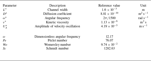
 \begin{equation} \textit{Sc} =\frac {\nu ^{\ast }}{D^{\ast }}, \quad \textit{Wo} = L^{\ast } \sqrt {\frac {\omega ^{\ast }}{\nu ^{\ast }}}. \end{equation}
Notice that
 $\omega = \textit{Sc} \textit{Wo}^2$
, where
 $\textit{Sc}$
is the Schmidt number and
 $\textit{Wo}$
is the Womersley number. Here,
 $\nu ^{\ast }$
is the kinematic viscosity of the fluid. For the choice of the characteristic velocity in (2.2), we use the velocity oscillation scale, namely
 $U^{\ast }_{c} = U_A^{\ast }$
.
The dimensionless Navier–Stokes equation and the boundary conditions for this case are
 \begin{equation} \frac {1}{\textit{Sc}} \frac {\partial u}{\partial t} = \frac {\partial ^2 u}{\partial y^2}, \quad u |_{y = 1} = \cos (\omega t), \quad u |_{y = 0} = 0. \end{equation}
The oscillatory velocity profile has a solution (Drazin & Riley Reference Drazin and Riley2006; Ding et al. Reference Ding, Hunt, McLaughlin and Woodie2021):
 \begin{equation} u (y, t) = {\textrm {Re}}\left [\textrm{e}^{\textrm{i} \omega t} \frac {\sinh \left ( \textrm{e}^{({ {\pi }/{4})} \textrm{i}} \textit{Wo} y \right )}{\sinh \left ( \textrm{e}^{({ {\pi }/{4})} \textrm{i}} \textit{Wo} \right )} \right ]. \end{equation}
Notice that
 $\textrm{e}^{({ {\pi }/{4})}\textrm{i}} = \sqrt {\textrm{i}} = ({\sqrt {2}}/{2}) (1+\textrm{i})$
. Here,
 $\textrm {Re}$
means taking the real part of the complex number.
For the two-time-variable system (3.6), we need to rewrite the velocity profile (4.3) in the form of the Fourier series of
 $t_1$
(see also the definition of
 $u_1$
in (3.2)) to calculate the expansion coefficient
 $B_{i, j}$
in (3.26):
 \begin{equation} u_1 (y, t_1) = \sum _{k = \pm 1} \frac {\sqrt {2 \pi }}{2} \left [ \frac {1}{\sqrt {2 \pi }} \textrm{e}^{\textrm{i} k t_1} \frac {\sinh \left ( \textrm{e}^{({ {\pi }/{4})} \textrm{i}} \sqrt {k} \textit{Wo} y \right )}{\sinh \left ( \textrm{e}^{({ {\pi }/{4})} \textrm{i}} \sqrt {k} \textit{Wo} \right )} \right ], \end{equation}
see also (5) of Ding et al. (Reference Ding, Hunt, McLaughlin and Woodie2021). Note that only one frequency is considered here. For the multiple-frequency case with more Fourier components (see also the paper by Vedel & Bruus Reference Vedel and Bruus2012), the solution procedure is similar but with more expansion coefficients for the ‘time’ variable
 $t_1$
.
Based on the experimental study by Ding et al. (Reference Ding, Hunt, McLaughlin and Woodie2021), we consider the transport problem of illuminated fluorescein dye in water. We perform the numerical simulation and analytical investigation based on the parameters listed in table 1. More cases of different parameter set-ups can be found in figure 9. In this case, the temporal evolution of the velocity profile is shown in figure 2. Due to the small Womersley number, the velocity profile is almost linear along the channel, namely, the boundary layer effect is weak.
Dimensional and dimensionless parameters in (2.2) and (4.1) for the transport of illuminated fluorescein dye in an oscillatory Couette flow of water. The parameters are partially taken from the experimental study by Ding et al. (Reference Ding, Hunt, McLaughlin and Woodie2021).

Dimensionless velocity profile
 $u(y,t)$
of the oscillatory Couette flow with the parameters listed in table 1.

4.2. Comparison with numerical simulation
To verify our analytical solution of the concentration moments, the Brownian dynamics simulation method (also known as the Monte Carlo method or random walk simulation) is adopted to obtain the numerical solutions. This simulation approach is widely applicable in various fields (Elhanati et al. Reference Elhanati, Dror and Berkowitz2023; Wu et al. Reference Wu, Zhan, Zhu, Zhang, Chang and Fu2026), as discussed in the comprehensive review by Berkowitz et al. (Reference Berkowitz, Cortis, Dentz and Scher2006). The numerical algorithm can be found in the recent paper by Ding et al. (Reference Ding, Hunt, McLaughlin and Woodie2021, § 3) (see also Wang et al. Reference Wang, Jiang, Chen, Tao and Li2021, Appendix A; Jiang & Chen Reference Jiang and Chen2021, Appendix B).
First, we need to find the corresponding stochastic differential equations (SDEs) for the original transport problem (2.1):
 \begin{align} \textrm{d} X_t &= u (Y_t, t) \; \textrm{d} t + \frac {\sqrt {2}}{\textit{Pe}} \; \textrm{d} W_1, \end{align}
 \begin{align} \textrm{d} Y_t &= \sqrt {2}\; \textrm{d} W_2, \end{align}
where
 $X_t$
and
 $Y_t$
are the random horizontal and transverse coordinates of the position of a particle, respectively. Here,
 $W_1$
and
 $W_2$
are independent standard Brownian motions.
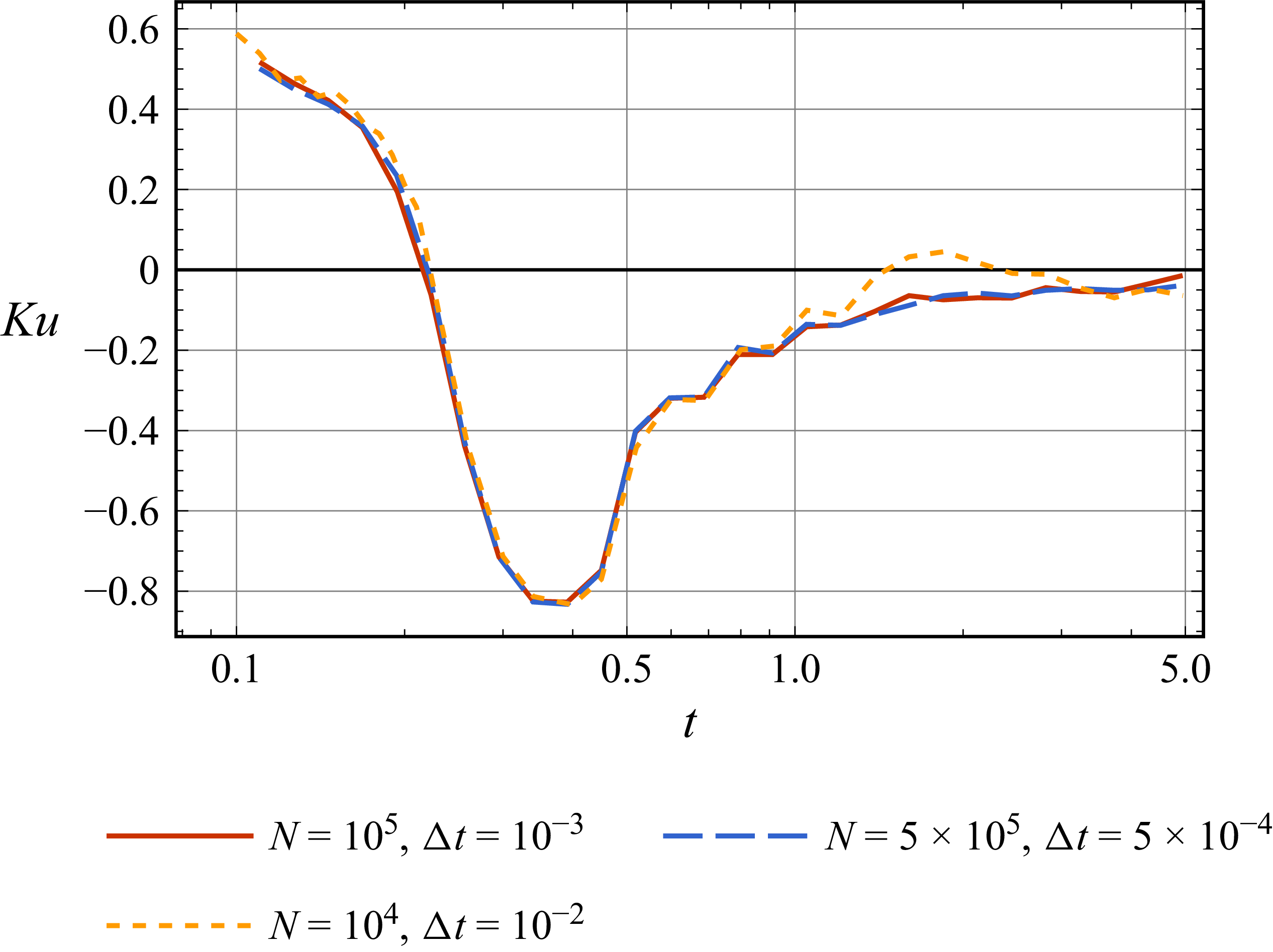
In our simulation, the Euler–Maruyama method is adopted to numerically solve the SDEs. The details are given in Appendix D. As shown in figure 8, after checking the independence of the time step (
 $\Delta t$
) and the number of particles (
 $N$
), we take
 $\Delta t = 10^{-3}$
and
 $N = 10^5$
. For the point-source release considered in figure 3, all particles are initially released at
 $x_0=0$
and
 $y_0 = 1$
, which corresponds to
 \begin{equation} C_{{{ini}}} = \delta (y-1) \end{equation}
in (2.1c ). The trajectories of particles are recorded. The positions of particles are used to statistically calculate concentration moments.
Comparison between the analytical solution of concentration moments and the numerical result by Brownian dynamics simulation: (a) the first-order moment of mean concentration distribution; (b) the variance of
 $\bar {C}$
; (c) the skewness of
 $\bar {C}$
; and (d) the kurtosis of
 $\bar {C}$
.
 $N_y$
denotes the number of eigenfunctions of
 $y$
used in the truncated summation of the analytical solution. The initial condition is a point-source release at
 $y_0 =1$
. Other parameters are listed in table 1.

For the analytical solution, the infinite summations in the solution expressions (such as (3.23)) need to be truncated for calculation or numerical evaluation (Barton Reference Barton1983). Only the first few eigenvalues (3.18), with indices
 $k$
and
 $m$
, and eigenfunctions (3.17) are used for the summations. First, for the Fourier series of
 $t_1$
for the oscillation in (3.17), we take
 $| k | \leqslant 4$
because we only consider concentration moments up to the fourth order for the discussion of kurtosis and the velocity profile is of one frequency. Higher-order moments will require more Fourier components of
 $t_1$
.
Second, for the trigonometric functions of
 $y$
in (3.17), the first
 $N_y$
eigenfunctions of
 $y$
(i.e.
 $m \leqslant N_y-1$
, because
 $m$
starts from 0) are used. We check the accuracy of the truncated summations by comparing the results of
 $N_y=4, 6, 8, 10$
. Take
 $N_y=8$
as an example. The total number of eigenfunctions
 $f_{m,k}$
is
 $8 \times (2\times 4 + 1) = 72$
. Then, we recollect all the eigenfunctions and eigenvalues into single-indexed lists
 $\{f_i(y, t_1)\}_{i=0}^{71}$
and
 $\{\lambda _i\}_{i=0}^{71}$
, and substitute them into the solution expressions of concentration moments.
As shown in figure 3, the analytical solutions of the transport characteristics of the mean concentration distribution
 $\overline {C}$
agree well with the numerical results, showing the correctness of the proposed auxiliary-time extension procedure. More comparisons under different parameter set-ups can be found in figure 9.
The truncation error may be large when
 $t$
is small, because a point-source-release initial condition (4.6) is considered. As shown in figure 3(c, d) for skewness and kurtosis, the curves of the results with
 $N_y=4$
and
 $N_y=6$
deviate from the numerical results in the initial stage. Namely, more eigenfunctions may be required for the higher-order moments. Generally speaking, the Dirac delta function in the initial condition (4.6) requires an infinite number of eigenfunctions of
 $y$
for the series summations in § 3.5 when
 $t\rightarrow 0$
. Fortunately, the truncation error will exponentially decrease as time increases (Barton Reference Barton1984). Note that the real part of the eigenvalue in (3.18) is
 $(m \pi )^2$
. Thus, the series summations in (3.23), (3.25), (C1) converge exponentially (with
 $\exp [-(m \pi )^2 t]$
), and the truncation error diminishes with a large enough
 $m$
. The results of
 $N_y=8$
and
 $N_y=10$
are close to the numerical results, as shown in figure 3. Therefore, we use
 $N_y=8$
in the following discussions. The linear–log plot (with a logarithmic scale of time) is used to highlight the alignment of curves in the initial short-time period, showing that the current configurations for the analytical and numerical solution procedures are sufficient.
We also compare the result of the Taylor dispersion coefficient (
 $D_T = \lim _{t \rightarrow \infty } \bar {\sigma }^2 / (2 t)$
) with the value obtained by Ding et al. (Reference Ding, Hunt, McLaughlin and Woodie2021, table 2, Trial 1). For
 $N_y=8$
, the dimensional
 $D_T$
is
 $5.38\times 10^{-9}\textrm {m}^2\,\textrm {s}^{-1}$
, which is consistent with the theoretical value of
 $5.39\times 10^{-9}\textrm {m}^2\,\textrm {s}^{-1}$
given by Ding et al. (Reference Ding, Hunt, McLaughlin and Woodie2021), although both values deviate from the experimental result of
 $4.26\times 10^{-9}\textrm {m}^2\,\textrm {s}^{-1}$
.
5. Effect of point-source release
With the auxiliary-time extension method being verified, one can investigate the effects of transport and flow parameters such as frequency, Schmidt number, Womersley number, etc. These basic effects have been discussed in many previous studies (Chatwin Reference Chatwin1975; Vedel & Bruus Reference Vedel and Bruus2012; Ding et al. Reference Ding, Hunt, McLaughlin and Woodie2021; Singh & Murthy Reference Singh and Murthy2023). In this study, our focus is the effects of the point-source release and the phase shift of velocity (see § 6) on the transport characteristics (especially the higher-order moments including skewness and kurtosis), which can also highlight the tractability of the auxiliary-time extension method.
In this section, we show the generality of the solution procedure by considering different initial conditions. The generality derives from Barton’s general solution expressions (Barton Reference Barton1983) because they are based on an arbitrary initial condition and thus have wide applicability. We consider the same oscillatory Couette flow and parameters as in § 4.2 (see table 1). Both the point-source release (
 $C_{{{ini}}} = \delta (y-y_0)$
) and the uniform release (
 $C_{{{ini}}} = 1$
) are considered. For the point-source case, three different initial positions
 $y_0 = 0$
,
 $y_0 = 0.5$
and
 $y_0 = 1$
are considered.
First, we discuss the effect of point-source release position on the first-order moment of the mean concentration distribution, as shown in figure 4(a, b). Obviously, the mean position of the solute cloud is strongly affected by the initial condition, while the effective drift velocity is weakly affected. Because the absolute value of the velocity at the upper wall is larger than that near the bottom wall, the effective drift velocity of the case with
 $y_0=1$
is larger than that of the case with
 $y_0=0$
. The curves of
 $u_d$
quickly overlap with each other after a short time (approximately half a period). Note that
 $u_d$
of the case with
 $y_0=0.5$
and the case with a transversely uniform release are nearly the same. This is because the Womersley number is so small that the velocity profile is nearly linear along the transverse direction, as shown in figure 2. Here,
 $u_d$
is the solute-weighted average velocity. The transport problem with a line-source release is nearly symmetric with respect to the centreline of the channel. Thus, its
 $u_d$
is nearly equal to the velocity value at the centreline, which is similar to the point-source case with
 $y_0=0.5$
.
Temporal evolution of (a) the mean longitudinal position, (b) the effective drift velocity, (c) the variance of mean concentration distribution and (d) the effective diffusion coefficient for different initial conditions.
 $y_0$
is the release position of the point-source release while ‘Line source’ denotes the uniform release. The parameters are listed in table 1.

For the second-order concentration moment, the temporal evolution of the variance of
 $\bar {C}$
and the effective diffusion coefficient is shown in figure 4(c, d). There is no doubt that the source-release form will affect these characteristics in the initial stage (Vedel et al. Reference Vedel, Hovad and Bruus2014). Similar to the effective drift velocity,
 $D_e$
of all the cases are nearly the same after a short time because the angular frequency
 $\omega$
is large. Note that
 $D_e$
of the case with
 $y_0=0$
is nearly the same as that of the case with
 $y_0=1$
. This is because of the quasi-linear velocity profile (with a small
 $\textit{Wo}$
). The spread of the solute cloud relative to the mean position is nearly symmetric for these two cases (or imagine the opposite case with an oscillating bottom wall instead of the upper wall). In addition, it is well known that
 $D_e$
can be negative in the transport problem with oscillatory flows (Chatwin Reference Chatwin1975; Smith Reference Smith1982a
; Yasuda Reference Yasuda1984), which can also be observed in figure 4(d). For the variance, all the curves are rising and are nearly overlapped with each other as
 $t$
increases.
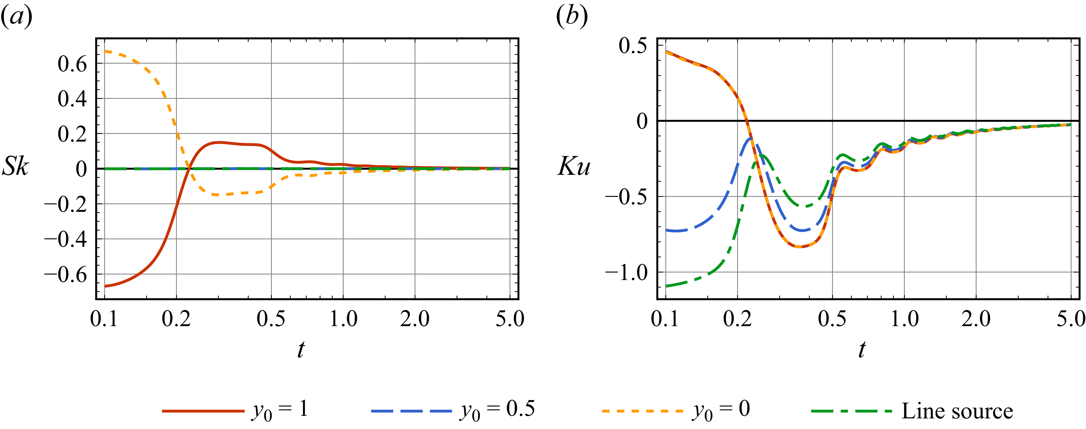
The results for the higher-order moments of
 $\bar {C}$
, skewness and kurtosis, are shown in figure 5. Similar to the case with a steady flow, both the skewness and kurtosis of the oscillatory case will still approach zero as
 $t$
increases because the Taylor dispersion regime is reached and
 $\bar {C}$
becomes Gaussian. As pointed out by Ding et al. (Reference Ding, Hunt, McLaughlin and Woodie2021, (28)), the decay rate of
 $\textit{Sk}$
for this single-frequency flow is
 $t^{-3/2}$
, faster than the steady case (
 $t^{-1/2}$
). However, when the flow has a non-zero net flow rate, the decay rate can be in the same order as the steady case. Moreover, the temporal evolution of skewness and kurtosis will be strongly affected by the initial condition.
Temporal evolution of (a) skewness and (b) kurtosis of the mean concentration distribution for different initial conditions.
 $y_0$
is the release position of the point-source release while ‘Line source’ denotes the uniform release. Other parameters are listed in table 1.

For skewness, the point-source case with
 $y_0=0.5$
and the line-source case have a nearly zero value of
 $\textit{Sk}$
, which means that
 $\bar {C}$
is nearly symmetric with respect to the mean position of the solute cloud. This is because the velocity profile is nearly linear along the transverse direction because the Womersley number is so small (see figure 2). As discussed for figure 4, the whole transport problem is quasi-symmetric with respect to the vertical line
 $x=0$
. Compared with the non-zero kurtosis in figure 5(b), a nearly zero
 $\textit{Sk}$
in the initial stage cannot ensure the Gaussianity of the concentration distribution. The Taylor dispersivity is neither enhanced nor inhibited because the flow configuration is unchanged. Skewness can be strongly affected by the initial condition.
For the point-source cases with
 $y_0=0$
and
 $y_0=1$
, their skewness values are nearly equal in magnitude but opposite in sign due to the quasi-symmetry of this specific transport problem. A positive
 $\textit{Sk}$
means that the distribution is upstream-leaning and vice versa. Note that the sign of skewness can be changed during the transport process due to the oscillation of the velocity profile.
The transient evolution of kurtosis is much more complicated, although the oscillation induced by the flow is not apparent. For the point-source cases with
 $y_0=0$
and
 $y_0=1$
, their kurtosis curves nearly overlap with each other due to the quasi-symmetry of this specific transport problem with a small
 $\textit{Wo}$
. When the time is small, the tailedness is larger than the Gaussian distribution (positive
 $\textit{Ku}$
, leptokurtic). However, the sign of kurtosis is changed during the transport process due to the velocity oscillation. For the other two cases, the absolute value of kurtosis of the line-source case is larger than that of a point source with
 $y_0=0.5$
. However, this trend can be reversed as time increases.
6. Effect of phase shift of velocity profile
Another benefit of the auxiliary-time extension method is that it can easily deal with the phase shift effect of the velocity field on the transport characteristics. Ding et al. (Reference Ding, Hunt, McLaughlin and Woodie2021) have discussed this effect on skewness’s sign change, with the transversely uniform release. Here, we further investigate the effect and show the result of other characteristics.
6.1. Solution procedure to address phase shift
First, we follow Ding et al. (Reference Ding, Hunt, McLaughlin and Woodie2021) and add a phase shift
 $s$
in the oscillatory velocity field as
 \begin{equation} u_s (y, t) \triangleq u (y, t + s). \end{equation}
Then, replace the original velocity field
 $u$
in (2.1a
) with the shifted velocity field
 $u_s$
.
Typically, one needs to re-solve the whole problem of the concentration moments to impose the phase shift. However, with the auxiliary-time extension method, we can directly obtain the solution with a simple transformation of the time variable
 $t_1$
. Notice that
 $t_1$
is imposed in (3.1) as
 $t_1 = \omega t$
. To address the phase shift, we impose the following time variables instead:
 \begin{equation} t_0 = t, \quad t_{1 s} = \omega (t + s). \end{equation}
Notice that
 $t_{1 s} = t_1 + \omega s$
. Then, similar to (3.2), we define
 $u_{s1}$
to replace the oscillatory velocity field for the shifted two-time-variable system and
 \begin{align} u_{s1} (y, t_{1 s}) & \triangleq u_s (y, t) = u (y, t + s)\notag \\ & = u \left(y, \frac {t_{1 s}}{\omega }-s + s\right) = u \left(y, \frac {t_{1 s}}{\omega }\right)\\ & = u_1 \left(y, t_{1 s}\right).\notag \end{align}
Namely, the function
 $u_{s1}$
is in the same form as
 $u_1$
. Thus, the governing equation for the shifted two-time-variable system is the same as that of the original system in (3.6).
To sum up, there is no need to re-solve the whole problem for the phase shift in flow velocity. The solution of the moments for the shifted two-time-variable system can be obtained by replacing
 $t_1$
with
 $t_{1 s}$
in the solution of the original two-time-variable system given in § 3.5. Namely,
 \begin{equation} P_{s n} (y, t_0, t_{1 s}) = P_n (y, t_0, t_{1 s}), \end{equation}
where
 $P_{s n}$
is the
 $n$
th-order moment of the shifted two-time-variable system. Based on (3.14), the
 $n$
th-order concentration moments
 $C_{s n}$
of the shifted problem is
 \begin{equation} C_{s n}(y, t) = P_{s n} (y, t_0, t_{1 s}) = P_n (y, t, \omega (t + s)). \end{equation}
Note that one could not obtain
 $C_{s n}(y,t)$
through
 $C_{n}(y,t)$
by simply replacing
 $t$
with
 $t + s$
. Fortunately, this could be done by
 $ P_n$
with
 $t_1$
replaced by
 $t_1 + \omega s$
, which can be considered as a benefit of the auxiliary-time extension method. In addition, as discussed by Ding (Reference Ding2025), the decay rate to the Taylor dispersion regime can be characterised by the non-zero eigenvalue with the smallest real part,
 $1/\textrm {Re}(\lambda )$
. Replacing
 $t_1$
would not influence the eigenvalue (3.18). Therefore, the decay rate to the Taylor dispersion regime is not affected by the phase shift.
We also perform the numerical verification for the phase shift effect, as shown in figure 11. The analytical result by (6.5) agrees well with the numerical result.
6.2. Results of transport characteristics
To illustrate the effect of the phase shift on the transport characteristics, we consider the same oscillatory velocity profile as that in previous sections, but with different phase shift
 $s=0, \pi /4, \pi , \pi /2, 3\pi /4$
. A point-source release is considered (
 $y_0 = 1$
). Note that the case with
 $s=\pi$
is the reverse case of the case with
 $s=0$
, due to the symmetry of the transport problem. Thus, only four cases are considered.
For the first-order moment of
 $\bar {C}$
and the effective drift, it can be seen in figure 6(a, b) that the effect of the phase shift is remarkable. Note that the effective drift is the solute-weighted average velocity, while the overall transverse distribution is not affected by the velocity field. Thus, the phase shift of the velocity will directly be reflected in the effective drift. It then leads to the accumulative change in the mean position of the solute cloud as time increases.
Temporal evolution of (a) the mean longitudinal position, (b) the effective drift velocity, (c) the variance of mean concentration distribution and (d) the effective diffusion coefficient for different phase shift
 $s$
. The initial condition is a point-source release at
 $y_0 = 1$
. Other parameters are listed in table 1.

Figure 6(c, d) shows the phase shift effect on the variance of
 $\bar {C}$
and the effective diffusion coefficient. Note that
 $D_e$
is initially zero because of the instantaneous release. The phase shift will change the time when
 $D_e$
reaches its maximum value. Then,
 $D_e$
will decay to the oscillatory state and reach the Reference TaylorTaylor dispersion regime. For the variance, similar to the effect of the initial condition discussed in § 5, the accumulative influence of the phase shift is weak and all the curves are nearly close to each other as
 $t$
increases.
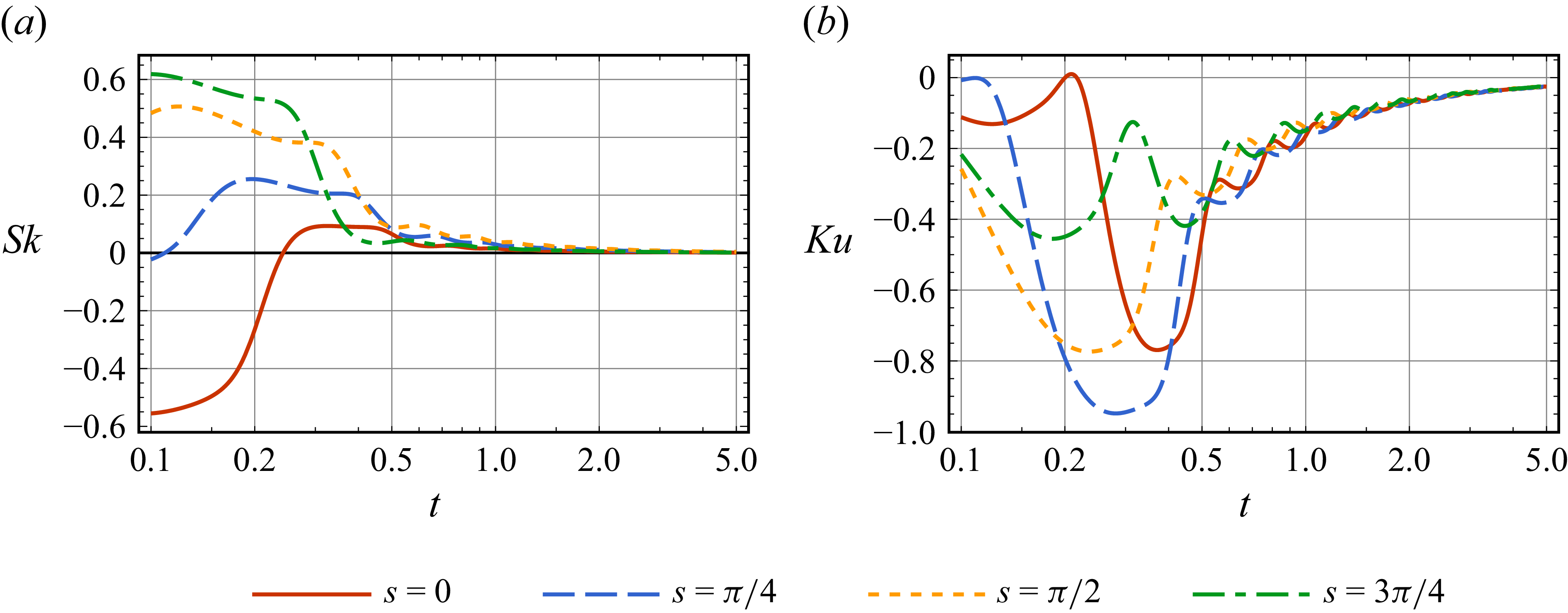
As discussed by Ding et al. (Reference Ding, Hunt, McLaughlin and Woodie2021), the phase shift can change the sign of skewness, which is clearly observed in figure 7(a). Unlike the line-source case of Ding et al. (Reference Ding, Hunt, McLaughlin and Woodie2021), the point-source case discussed here has a large non-zero skewness in the initial stage of the transport process. Thus, the oscillation of skewness is not apparent. However, the phase shift of the velocity field can still make a qualitative change in the asymmetry of the mean concentration distribution. If we compare the cases with
 $s=0$
and
 $s=\pi$
(not shown here), then the curves will be flipped with respect to the
 $t$
-axis due to the symmetric property of the transport problem.
Temporal evolution of (a) skewness and (b) kurtosis of the mean concentration distribution for different phase shift
 $s$
. The initial condition is a point-source release at
 $y_0 = 1$
. Other parameters are listed in table 1.

For kurtosis, the phase shift will change the sign of
 $\textit{Ku}$
, as shown in figure 7(b). The phase shift of the velocity field can be transferred to kurtosis, as the oscillation of
 $\textit{Ku}$
is apparent during the initial stage of the transport process. For the four considered cases, the temporal evolution curves have many intersections with each other even in the first period, showing the phase shift effect is complex.
7. Conclusions
Understanding the transient dispersion in oscillatory flows is crucial for many practical applications. The method of concentration moments is a powerful analytical tool for analysing the transport characteristics and has been well developed for the transport problems in steady flows. Barton (Reference Barton1983) has provided the general solution expressions for the first-few-order moments, using separation of variables. However, for unsteady flows, these results cannot be applied directly.
Many previous studies (Mukherjee & Mazumder Reference Mukherjee and Mazumder1988; Vedel & Bruus Reference Vedel and Bruus2012) had to use the moment method from the very beginning: re-solving the governing equation of moments. However, due to the complication induced by the time-periodic velocity field, the solution procedure is not as straightforward and general as that by Barton (Reference Barton1983). For higher-order statistics, the skewness has been derived only for a specific initial condition (Ding et al. Reference Ding, Hunt, McLaughlin and Woodie2021), while the solution for kurtosis remains analytically intractable, necessitating the use of numerical methods (Singh & Murthy Reference Singh and Murthy2023).
This manuscript proposes a novel analytical procedure by the introduction of an auxiliary oscillation time variable for the inherent oscillatory characteristics of the dispersion and extends the original transport problem to a two-time-variable problem, with the new time dimension virtually viewed as an additional ‘transverse’ space. Then, there is no need to re-solve the moment equation: the general solution expressions by Barton (Reference Barton1983) now can be used directly because the flow velocity becomes ‘steady’ after splitting the time variable. We remark that although the introduction of the time variables bears structural similarities to the two-time-scale homogenisation method, these two methods are fundamentally distinct in their underlying principles. The present method does not rely on either a small perturbation parameter or scale-separation analysis. The objective here is the concentration moments, not the long-time asymptotic concentration distribution (as in the homogenisation method).
The solution procedure for concentration moments is then greatly simplified to only two steps: (i) identifying the eigenvalue problem and (ii) substituting the eigenvalues and eigenfunctions in Barton’s expressions. This auxiliary-time extension treatment not only offers an intuitive physical perspective for the velocity oscillation, but also clarifies the solution structure of concentration moments. The complications encountered in previous studies can be avoided, making it feasible to investigate the temporal evolution of higher-order statistics and more applicable for complex transport problems in oscillatory flows. For example, this method has been extended to investigate the dispersion of swimming microorganisms in oscillatory channel flows (Wang et al. Reference Wang, Jiang, Zeng, Wu and Wang2025). The active dispersion phenomenon is of growing research interest (Peng Reference Peng2024; Caldag & Bees Reference Caldag and Bees2025; Fung, Caldag & Bees Reference Fung, Caldag and Bees2025; Zeng et al. Reference Zeng, Jiang, Guan, Lee and Chen2025a ). Future work can extend this method to oscillatory pipe flows and three-dimensional channel flows by changing the eigenfunction framework according to the cross-section geometry.
As a preliminary verification, we examine the transport problem in an oscillatory Couette flow. The numerical results by the Brownian dynamics simulation method are used for comparison and show good agreement with the analytical solutions by the auxiliary-time extension method.
Furthermore, to highlight the tractability of the auxiliary-time extension method, we investigate the effects of the point-source release and the phase shift of velocity on the transport characteristics, especially on higher-order statistics like skewness and kurtosis. The generality of the solution procedure derives from Barton’s general solution expressions for arbitrary initial conditions. For the phase shift of velocity, a simple transformation of the newly introduced time variable can be used to handle the phase shift effect without re-solving the moment equation. The oscillation of skewness is not apparent in the case with a point-source release. The phase shift of the velocity field can be remarkably transferred to the temporal evolution of kurtosis. Both these two effects can change the sign of skewness and kurtosis, qualitatively affecting the asymmetry and the tailedness of the mean concentration distribution.
Acknowledgements
The authors would like to thank Dr Bohan Wang for constructive discussions.
Funding
This work is supported by the Science and Technology Development Fund (FDCT) of Macao SAR (Project Nos. 0025/2024/RIA1, 0018/2023/ITP1, 0031/2024/AMJ and 0001/2024/NRP) and the National Natural Science Foundation of China (Grant No. 52079001).
Declaration of interests
The authors report no conflict of interest.
Appendix A. Governing equations of moments
To derive the governing equation of concentration moments, it is assumed that concentration decays exponentially (Aris Reference Aris1956; Li et al. Reference Li, Wang, Jiang, Zeng, Li and Chen2017). Integrating (2.1a
), according to the definition of
 $C_n$
in (2.5), and using the integration by parts formula, we have
 \begin{equation} \frac {\partial C_n}{\partial t} - \frac {\partial ^2 C_n}{\partial y^2} = n \, u(y, t) C_{n - 1} + \frac {n (n-1)}{\textit{Pe}^2}C_{n - 2} \end{equation}
for
 $n=0,1,2,\ldots$
. Notice that
 $C_{-1}=C_{-2}=0$
are auxiliary terms. The boundary conditions of
 $C_n$
are the same as that of
 $C$
in (2.1b
):
 \begin{equation} \left . \frac {\partial C_n}{\partial y} \right |_{y = 0} = \left . \frac {\partial C_n}{\partial y} \right |_{y = 1} = 0. \end{equation}
For the initial condition, according to (2.1c ), we have
 \begin{equation} C_n | _{t = 0} = \left \{\begin{array}{ll} C_{{{ini}}} (y), & n = 0,\\ 0 , & n = 1, 2, \ldots . \end{array} \right . \end{equation}
Note that the governing equation (A1) of
 $C_n$
contains the time-dependent velocity field
 $u(y,t)$
as a source term on the left side. Thus, obtaining time-integral solutions for
 $C_n$
is more complicated compared with steady flow cases, particularly for higher-order moments.
Appendix B. Solution of the eigenvalue problem
For the eigenvalue problem (3.16), one can use the method of separation of variables to obtain the solution.
Assume that the solution form of the eigenfunction
 $f$
is
 \begin{equation} f(y, t_1) = Y(y) T_1(t_1). \end{equation}
Substituting it into (3.16a ) yields
 \begin{equation} - \omega \frac {1}{T_1} \frac {\textrm{d} T_1}{\textrm{d} t_1} + \frac {1}{Y} \frac {{d}^2 Y}{\textrm{d} y^2} = - \lambda . \end{equation}
Note that
 $Y$
depends only on
 $y$
,
 $T_1$
depends only on
 $t_1$
and the eigenvalue
 $\lambda$
is a constant. Therefore,
 \begin{equation} \frac {1}{Y} \frac {\textrm{d}^2 Y}{\textrm{d} y^2} = - \lambda + \omega \frac {1}{T_1} \frac {\textrm{d} T_1}{\textrm{d} t_1} = -\lambda _y, \end{equation}
where
 $\lambda _y$
is a constant. We can also introduce another constant
 \begin{equation} \lambda _{t_1}=\frac {\lambda -\lambda _y}{\omega } \end{equation}
for
 $T_1$
.
Note that the boundary conditions (3.16b
), (3.16c
) are also separable. Thus, for
 $Y(y)$
, we have
 \begin{align} \frac {\textrm{d}^2 Y}{\textrm{d} y^2} &= - \lambda _y Y, \end{align}
 \begin{align} \left . \frac {\partial Y}{\partial y} \right |_{y = 0} &= \left . \frac {\partial Y}{\partial y} \right |_{y = 1} = 0. \end{align}
According to the boundary conditions, the solution of
 $Y(y)$
is a trigonometric function. We have
 \begin{equation} Y(y)= a_m \cos (m \pi y) + b_m \sin (m \pi y), \quad \lambda _y = (m \pi )^2, \end{equation}
and
 $m=0,1,2,\ldots$
. Here,
 $b_m = 0$
and
 $a_m$
is a constant coefficient.
For
 $T_1$
, we have
 \begin{align} \frac {\textrm{d} T_1}{\textrm{d} t_1} &= \lambda _{t_1} T_1, \end{align}
 \begin{align} T_1 |_{t_1=0} &= T_1 |_{t_1 = 2 \pi }. \end{align}
Due to the periodic condition (B7b
), the solution of
 $T_1$
is the complex Fourier series. We have
 \begin{equation} T_1 = a_k \exp (\textrm{i} k t_1), \quad \lambda _{t_1} = \textrm{i} k, \end{equation}
where
 $k = 0, \pm 1, \pm 2, \ldots$
and
 $a_k$
is the constant coefficient.
Finally, returning to (B1), we obtain
 \begin{equation} f (y, t_1) = a_m \cos (m \pi y) a_k \exp (\textrm{i} k t_1), \end{equation}
and the corresponding eigenvalue (B4)
 \begin{equation} \lambda = \lambda _y + \omega \lambda _{t_1} = (m \pi )^2 + \textrm{i} k \omega . \end{equation}
Appendix C. Solution of second-order moment
For the second-order moment, based on (2.14) of Barton (Reference Barton1984), the solution is
 \begin{align} {{P}}_2 (y, t_0, t_1) = & \sum ^{\infty }_{i=0} a_i B_{i, i}^2 t_0^2 \textrm{e}^{- \lambda _i t_0} {f}_i + \sum ^{\infty }_{\substack {i,j=0 \\ j\neq i}} \frac {2 E_{i, j} a_j (\textrm{e}^{- \lambda _j t_0} - \textrm{e}^{- \lambda _i t_0}) }{\lambda _i - \lambda _j} {f}_i +\sum ^{\infty }_{i=0} 2 a_i E_{i,i} t_0 \textrm{e}^{-\lambda _i t_0} f_i \notag \\ &+\sum ^{\infty }_{\substack {i,j,k=0 \\ k\neq j, k\neq i}} \frac {2 a_k B_{j, k} B_{i, j} (\textrm{e}^{- \lambda _k t_0} - \textrm{e}^{-\lambda _i t_0}) }{(\lambda _k - \lambda _i) (\lambda _k - \lambda _j) }{f}_i +\sum ^{\infty }_{\substack {i,j=0 \\ i\neq j}} \frac {2 a_i B_{j, i} B_{i, j} t_0 \textrm{e}^{- \lambda _i t_0} }{\lambda _j -\lambda _i} {f}_i \notag \\ &+\sum ^{\infty }_{\substack {i,j,k=0 \\ k\neq j, j\neq i}} \frac {2 a_k B_{j, k} B_{i, j} (\textrm{e}^{- \lambda _j t_0} - \textrm{e}^{-\lambda _i t_0}) }{(\lambda _k - \lambda _j) (\lambda _i - \lambda _j)}{f}_i +\sum ^{\infty }_{\substack {i,k=0 \\ k\neq i}} \frac {2 a_k B_{i, k} B_{i, i} t_0 \textrm{e}^{- \lambda _i t_0} }{\lambda _k -\lambda _i} {f}_i \notag \\ &+\sum ^{\infty }_{\substack {i,j=0 \\ j\neq i}} \frac {2 a_j B_{j, j} B_{i, j} \left[\textrm{e}^{- \lambda _i t_0} - \textrm{e}^{-\lambda _j t_0} + (\lambda _i - \lambda _j) t_0 \textrm{e}^{- \lambda _j t_0}\right]}{(\lambda _j - \lambda _i)^2} {f}_i, \end{align}
where
 $E_{i, j}$
is the coefficient related to the diffusion coefficient
 $D$
,
 \begin{align} E_{i, j} &\triangleq \langle {f}_i, D {f}_j \rangle \notag \\ &= \int ^{2 \pi }_0 \int ^1_0 f_i^{\star } (y, t_1) D f_j (y, t_1) \, \textrm{d} y \,\textrm{d} t_1 \\ &= D \delta _{i j}\notag \end{align}
for
 $i, j = 0, 1, \ldots$
. Note that
 $D=1/\textit{Pe}^2$
for the transport problem considered in (3.6).
For the third- and fourth-order moments, the readers can refer to (3.17) of Barton (Reference Barton1983), an analytical expression of the third-order moment can also be found in Appendix A of Yang et al. (Reference Yang, Jiang, Wu, Wang, Wu, Zhang and Zeng2021). Their expressions are too long to be reproduced here. For practical purposes, readers can refer to the study of Jiang et al. (Reference Jiang, Zeng, Fu and Wu2022), with a Mathematica notebook provided at https://doi.org/10.5281/zenodo.14927459.
Appendix D. Numerical stochastic differential equations
D.1. Euler–Maruyama scheme
We use the Euler–Maruyama scheme to solve the SDEs (4.5). Let
 $X_n$
and
 $Y_n$
denote the position of a particle at the
 $n$
th time step
 $t_n=n\Delta t$
. We have
 \begin{align} X_{n + 1} &= X_n + u (Y_n, t_n) \Delta t + \frac {\sqrt {2 \Delta t}}{\textit{Pe}} \Delta W_1, \end{align}
 \begin{align} Y_{n + 1} & = Y_n + \sqrt {2 \Delta t} \Delta W_2, \end{align}
where
 $\Delta W_1$
and
 $\Delta W_2$
are random variables generated at each time step. They satisfy the standard normal distribution, i.e.
 $\Delta W_1 \sim \textrm{N}(0, 1)$
and
 $\Delta W_2 \sim \textrm{N}(0, 1)$
. Here,
 $\textrm{N}$
denotes the normal distribution. In our code, we add
 $t_{n+1}=t_n + \Delta t$
to (D1) such that the whole system is autonomous.
On the channel walls (
 $y=0$
and
 $y=1$
), the specular reflection model (billiard-like reflection) is adopted to simulate the non-penetration boundary condition (2.1b
). If a particle exceeds the boundaries after the calculation at the
 $n+1$
time step, it is reflected back to the channel:
 \begin{align} Y_{n + 1} \rightarrow - Y_{n + 1} \quad \text{if} \; Y_{n + 1} \lt 0, \end{align}
 \begin{align} Y_{n + 1} \rightarrow 2 - Y_{n + 1} \quad \text{if} \; Y_{n + 1} \gt 1. \end{align}
For the initial condition, we set
 $X_0 = 0$
and
 $Y_0 = 1$
for a point-source release at
 $y_0 = 1$
. For the uniform release (
 $C_{{{ini}}} = 1$
),
 $X_0$
is a random variable generated from the uniform distribution on the interval
 $[0, 1]$
.
The numerical error of the Euler–Maruyama scheme is mainly determined by the time step
 $\Delta t$
(which scales as
 $\mathcal{O} (\sqrt {\Delta t})$
) and the number of particles
 $N$
. In figure 8, we have compared the numerical results of kurtosis with different
 $\Delta t$
and
 $N$
. The curves of the result of
 $N=10^5$
and
 $\Delta t = 10^{-3}$
are nearly overlapped with the result of
 $N=5 \times 10^5$
and
 $\Delta t = 5 \times 10^{-2}$
, which means that the numerical independence had been achieved at this set-up. The result of
 $N=10^4$
and
 $\Delta t = 10^{-2}$
considerably deviates from the other two when
 $t$
is large, which means that the time step is too coarse. Therefore, we use
 $N=10^5$
and
 $\Delta t = 10^{-3}$
for the numerical simulations. Python code is provided at https://doi.org/10.5281/zenodo.16781949.
Numerical results of kurtosis of the mean concentrations distribution under different set-up of the number of particles (
 $N$
) and the time step (
 $\Delta t$
). The initial condition is a point-source release at
 $y_0 = 0.75$
. Other parameters are listed in table 1.

D.2. Comparisons under different parameter setups
In figure 3, we compare the analytical and numerical results under one single parameter set-up. Some parameters used in the comparison (listed in table 1) are small. The proposed two-time-variable method does not require any small parameters or scale-separation conditions as the two-scale homogenisation method does. To demonstrate this point more clearly, we compare the results under different parameter set-ups in figure 9. We take the first-order moment of mean concentration distribution as an example. Both the analytical results of the cases with a smaller angular frequency and with a much larger angular frequency agree well with the numerical results. The cases with different magnitude values of
 $\textit{Pe}$
,
 $\textit{Wo}$
and
 $\textit{Sc}$
are also consistent across the analytical and numerical results.
More comparisons between the analytical and numerical results under different parameter set-ups. The first-order moment of mean concentration distribution (
 $\bar {\mu }_x$
) is shown. The initial condition is a point-source release at
 $y_0 = 0.75$
. With fixed parameters listed in table 1, the modified parameter in each case is: (a)
 $\omega =1$
; (b)
 $\omega =100$
; (c)
 $\textit{Wo}=1$
; (d)
 $\textit{Wo}=10$
; (e)
 $\textit{Pe}=1$
; (f)
 $\textit{Pe}=10$
; (g)
 $\textit{Sc}=10$
; and (h)
 $\textit{Sc}=100$
.

The comparison under a continuous change of parameters is shown in figure 10. Because the angular frequency
 $\omega$
can be considered as a distinctive parameter for oscillatory flows compared with the steady case, we choose
 $\omega$
for the comparison. Moreover, only the results at
 $t=1$
are plotted for a more direct comparison.
Comparisons between the analytical and numerical results for different angular frequency
 $\omega$
at
 $t=1$
: (a) the first-order moment of mean concentration distribution; (b) the variance of
 $\bar {C}$
; (c) the skewness of
 $\bar {C}$
; and (d) the kurtosis of
 $\bar {C}$
. The initial condition is a point-source release at
 $y_0 = 0.75$
. Other parameters are listed in table 1. Note that
 $\textit{Wo}$
is fixed.

Figure 10 shows the curves of the basic dispersion characteristics as
 $\omega$
increases, which can be considered as a local sensitivity of
 $\omega$
. The analytical results agree well with the numerical ones by random walk simulations. Moreover, there is an overall decreasing trend of the variance in figure 10(b). Note that the Womersley number
 $\textit{Wo}$
is fixed in the comparison (and thus the Schmidt number
 $\textit{Sc}$
changes as
 $\omega$
varies), namely, the spatial shape of the Stokes layer remains unchanged. The oscillation can inhibit the dispersion process. This has been investigated by Ding et al. (Reference Ding, Hunt, McLaughlin and Woodie2021, figure 2): the Taylor dispersivity decreases as
 $\omega$
increases when
 $\textit{Wo}$
is fixed.
D.3. Phase shift
We also perform the numerical simulation for the case with a phase shift of the velocity field. Figure 11 shows the numerical verification for the treatment of the phase shift effect presented in § 6.1. The analytical solutions of the transport characteristics agree well with the numerical results.
Comparison between the analytical solution of concentration moments and the numerical result for the phase shift effect: (a) the first-order moment of mean concentration distribution; (b) the variance of
 $\bar {C}$
; (c) the skewness of
 $\bar {C}$
; and (d) the kurtosis of
 $\bar {C}$
. The initial condition is a point-source release at
 $y_0 = 0.75$
. Other parameters are listed in table 1.