





Impact statement
Deploying long-duration energy storage is critical for mitigating the intermittency of renewable energy generation and enabling a more resilient low-carbon energy system. Compressed air energy storage (CAES) represents a promising technology in this field; however, its widespread adoption can be hindered by the substantial capital investment associated with large-scale thermal storage tanks. This study addresses this challenge by proposing a multi-tank storage concept that has the potential to reduce construction costs while maintaining reliable system operation. The proposed approach provides new insights into the redesign of large-scale thermal storage systems through improved integration of multiple storage units rather than simply increasing the size of individual components. By allowing multiple smaller tanks to function as an integrated storage unit, this concept enhances flexibility in system design, manufacturing and future capacity expansion. Such flexibility is particularly valuable for large energy storage facilities, where cost reduction, scalability and operational reliability are key factors influencing deployment. The findings contribute to the development of more economically viable CAES systems and support the transition towards sustainable energy infrastructures. Furthermore, the design principles presented in this study may be extended to other large-scale thermal and fluid storage technologies that require coordinated operation among multiple storage units.
Introduction
In response to the escalating challenges of climate warming and the global environmental crisis, an increasing number of governments around the world have introduced comprehensive policy frameworks and financial incentives to accelerate the advancement and deployment of renewable energy technologies, solar and wind power, in particular (Hassan et al., Reference Hassan, Viktor, Al-Musawi, Ali, Algburi, Alzoubi, Al-Jiboory, Sameen, Salman and Jaszczur2024; Noh et al., Reference Noh, Jafarinejad and Anand2024; Zhang et al., Reference Zhang, Padhan, Singh and Gupta2024). Despite these efforts, the inherent intermittency and variability of renewable energy sources continue to pose significant obstacles to their widespread and stable integration into the energy grid, thereby limiting their large-scale commercialization potential (Notton et al., Reference Notton, Nivet, Voyant, Paoli, Darras, Motte and Fouilloy2018; Ekoue et al., Reference Ekoue, Woerman and Clastres2025). It is widely acknowledged that the adoption of energy storage technologies represents an effective strategy to enhance the reliability, stability and overall performance of renewable energy systems. As the global utilization of renewable energy continues to expand, the energy storage sector has witnessed a remarkable and sustained growth trend over the past few decades. In 2024, the global market size of energy storage technologies reached approximately USD 90.36 billion (Fortune Business Insights, 2025), and it is forecasted to grow significantly, reaching USD 231.06 billion by 2032, with a projected compound annual growth rate of 12.45% (Fortune Business Insights, 2025). Among various energy storage options, compressed air energy storage (CAES) systems are widely recognized for their suitability in meeting large-scale and long-duration storage demands (Government of Canada, 2024).
The fundamental principle of a CAES system is to use off-peak electricity to compress and store air, which is later released and expanded to generate electricity during periods of peak demand (Burian and Dančová, Reference Burian and Dančová2023). To achieve this, a typical CAES system primarily comprises electric motors, compressors, expanders and air storage units. However, due to the challenges in maintaining ideal isothermal conditions during compression and expansion, significant heat losses occur in these processes, which can adversely affect the overall system performance (Mitra et al., Reference Mitra, Mahato, Nag and Kumar2022). Among the various improvements proposed for CAES systems, the integration of intercooling and preheating subsystems has proven to be one of the most effective approaches for enhancing system efficiency (Komba et al., Reference Komba, Haisong, Liwoko and Mwakipunda2025). For example, Chen et al. (Reference Chen, Hu, Sheng and Xie2017) introduced an additional air-conditioning unit following the intercooling stage, which ensures that the compressed air reaches ambient temperature before entering the subsequent compression stage. In a system configuration with four-stage compressors and two-stage expanders, their design achieved an increase of over 3% in round-trip efficiency compared to conventional CAES systems (Chen et al., Reference Chen, Hu, Sheng and Xie2017). Additionally, the McIntosh CAES plant, equipped with three-stage compressors and two-stage expanders, utilizes preheating of the air before expansion, resulting in an overall efficiency of up to 53% (Rabi et al., Reference Rabi, Radulovic and Buick2023).
Due to its low cost and excellent thermal capacity, water is commonly used as the thermal medium in the intercooling and preheating subsystems of large-scale CAES projects (Wang et al., Reference Wang, Carriveau, Ting, Brown and McGillis2025). As a result, water storage tanks have become essential components in many CAES system configurations. For instance, Wang et al. (Reference Wang, Zhang, Yang, Zhou and Wang2016) integrated a thermal energy storage unit into a CAES system, employing water as the working medium. The thermal energy storage unit absorbs the heat generated during compression, with the stored water temperature reaching as high as 108.6 °C. During the discharging process, the stored hot water is utilized to preheat the compressed air to 100 °C before it enters the expander stage. Additionally, Mazloum et al. (Reference Mazloum, Sayah and Nemer2017) proposed a novel isobaric adiabatic CAES system featuring two core thermal components: a pressurized hot water tank and multiple combined air/water tanks. The hot water tank serves two purposes – recovering thermal energy during the charging phase and supplying heat to raise the temperature of the compressed air before expansion during discharging. By maintaining the tank under pressure, water evaporation is effectively suppressed. The air/water tanks facilitate adiabatic storage under nearly constant pressure, thereby enhancing the energy density of the overall storage system. Similarly, He et al. (Reference He, Wang, Ge, Liu and Zhang2023) implemented a pressurized water thermal energy storage system to improve the efficiency of an open-type isothermal compressed air energy storage configuration. In their design, a low-pressure water tank recovers heat from the compressors and the collected thermal energy is further boosted using electric heaters. The heated water is then transferred to a high-pressure tank for storage and subsequently used to preheat the compressed air during the discharging stage. Their findings indicated that the CAES subsystem could achieve an efficiency of up to 91.9% with the pressurized water thermal energy storage system in operation. Furthermore, Vladuca et al. (Reference Vladuca, Borzea, Ionescu, Ţăranu and Ciobanu2020) introduced and assessed the first real-world CAES application in Romania. The system incorporates a 50 m3 water reservoir, which enhances compressor and expander performance during both charging and discharging operations.
Among various CAES applications, a wide range of water storage tank shapes can be observed in the thermal subsystems, including spherical tanks, cylindrical tanks and capsule-shaped designs. Given the critical role of water storage in the thermal management of CAES systems, careful consideration of tank design – especially in terms of thermal performance, pressure resistance and cost-effectiveness – has become increasingly important. Under laminar natural convection conditions, Yang et al. (Reference Yang, Chen, Wang, Sheng and Wang2016) conducted a comparative study on the thermal performance of water tanks with 10 different geometries operating in static mode. Simulation results indicated that a tank’s thermal storage capacity is primarily governed by its surface-area-to-volume ratio. In this context, spherical tanks exhibited the highest thermal capacity due to their minimal surface area per unit volume, while cylindrical tanks showed the lowest. Intermediate shapes, such as capsule shaped tanks, demonstrated moderate thermal performance. In addition to thermal considerations, mechanical stress caused by internal pressure, particularly during hot water storage, must be addressed. Therefore, pressure resistance is a key factor in determining optimal tank shape. It is widely acknowledged that the sphere represents the most efficient geometry for withstanding internal pressure uniformly (Oyelami and Olusunle, Reference Oyelami and Olusunle2019). However, due to the complexity of fabrication and associated high costs, fully spherical tanks are rarely used in pressurized applications (Oyelami and Olusunle, Reference Oyelami and Olusunle2019). As a practical alternative, a capsule shaped design – consisting of a cylindrical body with two spheroidal end caps – is commonly adopted. This configuration offers a balance between structural strength and manufacturing feasibility, making it a preferred choice for pressurized thermal storage in CAES systems.
For capsule shaped tanks, the loading pressure capacity is primarily determined by the design of the end caps. Based on simulation studies, Bică et al. (Reference Bică, Ţălu and Ţălu2017) demonstrated that capsule shaped tanks equipped with ellipsoidal heads exhibit superior performance in terms of stress distribution and structural deformation when compared to other head designs, such as tori-spherical and flat caps. In addition to mechanical performance, construction costs vary significantly depending on both the head geometry and the materials used. Altinbalik and İsencik (Reference Altinbalik and İsencik2016) conducted an economic analysis of capsule shaped tanks incorporating three different head designs and two commonly used structural materials. Assuming a constant storage volume, their results revealed that hemispherical head designs reduce the overall height of the tank compared to ellipsoidal and tori-spherical heads. When fabricated from SA-516 GR70 steel, tanks with hemispherical heads achieve material savings of approximately 7% and 21% relative to ellipsoidal and tori-spherical designs, respectively. Furthermore, when using stainless steel SA-240 304L, the material savings become even more significant – up to 27% compared to the ellipsoidal and tori-spherical alternatives. These findings suggest that head design and material selection not only influence mechanical performance but also play a crucial role in optimizing cost-effectiveness and structural efficiency in pressurized capsule shaped tank applications.
Recent studies on water storage design have primarily focused on the performance evaluation of individual tank geometries (Altinbalik and İsencik, Reference Altinbalik and İsencik2016; Yang et al., Reference Yang, Chen, Wang, Sheng and Wang2016; Bică et al., Reference Bică, Ţălu and Ţălu2017; Oyelami and Olusunle, Reference Oyelami and Olusunle2019). However, in large-scale CAES systems, multiple water tanks are typically deployed to meet the substantial thermal storage requirements. While significant attention is often given to the capital costs associated with the power island, such as compressors and expanders, the expenses related to the balance of plant, engineering, procurement and construction also represent a major portion of the total investment. According to Siemens’ reference data (Mongird et al., Reference Mongird, Viswanathan, Alam, Vartanian and Sprenkle2020), approximately 40% of the overall capital cost in a CAES project is attributed to balance of plant, engineering, procurement and construction activities. As the number of water tanks increases, the system demands additional auxiliary components, including valves, pipelines, control sensors and support structures. These added elements further escalate both material and labor costs. Therefore, it becomes essential to optimize the spatial layout and system integration of the multi-tank configuration in CAES systems. A well-planned layout can significantly reduce the complexity and installation costs associated with auxiliary equipment, ultimately contributing to improved economic feasibility and system reliability.
In this study, a novel layout strategy is proposed for a CAES system equipped with 24 capsule shaped hot water storage tanks. In the proposed configuration, the 24 tanks are organized into several blocks, with each block comprising multiple tanks connected in series. To reduce the overall cost of the water storage subsystem, all tanks within a given block share a single set of auxiliary components, such as valves, sensors and pipelines. This design aims to promote synchronized variations in temperature, pressure and water level among the tanks within each block throughout both the charging and discharging processes. To assess the feasibility of this layout, an equilibrium thermodynamic model was developed to determine whether it is necessary to interconnect the vapor zones of the tanks within each block during operation. Moreover, in order to further minimize auxiliary equipment costs, the total number of blocks should be reduced as much as possible without compromising performance. Based on the developed model, three different layout configurations were analyzed and compared: (1) 12 blocks containing 2 tanks each, (2) 8 blocks with 3 tanks each and (3) 6 blocks consisting of 4 tanks each. This study also explored how the diameter of the interconnecting pipes influences the degree of synchronization in thermofluidic property changes – such as pressure and temperature – among tanks within the same block.
Thermodynamics model of a water tank system
In a CAES system, the primary function of the hot water tank is to raise the temperature of high-pressure air before it enters the expansion turbines, thereby enhancing the overall system efficiency (Budt et al., Reference Budt, Wolf, Span and Yan2016). Due to the potential for boiling, a certain level of internal pressure is typically required when storing hot water, necessitating pressure-rated container designs. According to the design specifications outlined by Hydrostor Inc., capsule shaped water tanks (as depicted in Figure 1) serve as the hot water reservoirs in such systems. This tank configuration offers a practical balance between pressure resistance and economic feasibility. Structurally, each tank consists of a metallic shell for structural integrity, a thermal insulation layer to reduce heat loss and specifically designed inlet and outlet ports for fluid management during operation. To investigate the transient behavior of such hot water tanks, it is crucial to establish governing equations that incorporate both energy conservation and mass balance principles. The accuracy and reliability of the simulation are also highly dependent on the appropriate selection of the time step, which significantly affects numerical stability, convergence behavior and computational efficiency. Therefore, this section focuses on determining a time step that achieves an optimal balance between solution accuracy and simulation runtime, ensuring both precision and practicality in the modeling process.
Schematic of a capsule shaped water tank.

Figure 1. Long description
The figure consists of two parts illustrating a vertical capsule-shaped water tank. On the left is a 3D cutaway schematic showcasing the tank resting on a metal stand. Labels point out the top inlet port, the internal gas zone, the water zone below and a double-layered wall consisting of an outer insulation layer and an inner metal layer. A bottom outlet port is located at the lower left. On the right is a 2D geometric diagram set against a vertical coordinate axis with the origin ‘O’ at the cylinder center. Key height levels are marked along the axis: the top dome apex at L/2, the upper cylinder transition line at L′/2, the lower cylinder transition line at -L′/2 and the bottom dome apex at -L/2. The inner diameter of the tank is labeled as D. The lower half of the 2D sketch contains horizontal lines representing the water level within the tank.
1-D thermodynamic model of a water tank
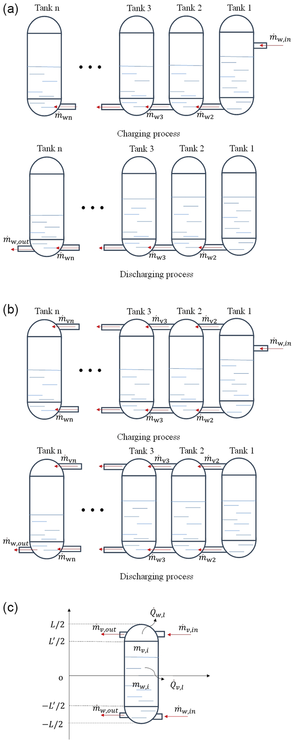
Figure 2a,b shows two kinds of multi-tank models connected in series: with and without vapor-zone connections. Normally, a full cycle consists of charging, stand-by and discharging processes. The stand-by period typically occurs between the charging and discharging stages rather than involving an immediate flow reversal. Therefore, the transient dynamic effects associated with abrupt flow reversal are expected to be negligible in this context. In addition, the main objective of this study is to evaluate whether connecting the steam regions among different tanks is necessary during the charging and discharging processes. To this end, the transient model primarily includes two stages: charging and discharging. Under these conditions, the system can be reasonably simplified as an open system. To further reduce model complexity, several assumptions are introduced. An equilibrium thermodynamic approach is adopted, meaning that at each time step, the water and steam within the tank are assumed to exist in a saturated state. Additionally, the model neglects internal temperature gradients as well as thermal resistances at the interfaces between different metal shells and the insulation layer.
Schematics of working processes in multi-capsule shaped water tanks: (a) multi-tanks without gas zone connections, (b) multi-tanks with gas-zone connections and (c) an open system analysis of a general capsule shaped tank.

Figure 2. Long description
Panel a shows two rows of tanks labeled Tank 1, Tank 2, Tank 3, and Tank n. In the Charging process, fluid enters Tank 1 from the top right via m dot sub w,in and flows through a bottom pipe connecting all tanks. In the Discharging process, fluid exits from the bottom left of Tank n via m dot sub w,out.
Panel b shows a similar multi-tank setup but with two horizontal pipes connecting the tanks at both the top and bottom. In the Charging process, fluid enters Tank 1 from the middle right. In the Discharging process, fluid exits from the bottom left of Tank n.
Panel c is a detailed schematic of a single tank centered on a coordinate system with a vertical y-axis and horizontal x-axis.
• At the top (y = L/2), an arrow m dot sub v,in enters from the right and Q dot sub w,l exits from the top dome.
• Just below (y = L prime/2), m dot sub v,out exits to the left.
• The upper interior is labeled m sub v,i.
• The center origin o marks the transition to the lower interior labeled m sub w,i, where Q dot sub v,l exits to the right.
• Near the bottom (y = -L prime/2), m dot w,out exits to the left.
• At the base (y = -L/2), m dot w,in enters from the right.
As illustrated in Figure 2c, the change in internal energy of the open system is governed by the combined energy variations of the liquid water and vapor phases between time steps ‘i’ and ‘i + 1’. The system interacts thermally through several mechanisms, including energy input from an external heater, mass transfer of water and vapor during both charging and discharging processes and heat losses through the wet and dry walls of the tank. According to the principle of energy conservation for open systems, the variation in internal energy equals the algebraic sum of energy input, energy output and net heat sources, as expressed in Eq. (1).

in which,
$ \dot{m} $
 represents the mass flow rate, and the subscripts ‘w’, ‘v’, ‘in’ and ‘out’ refer to water, vapor, inlet and outlet, respectively. The symbols h and u denote the specific enthalpy and specific internal energy. The thermal energy supplied by the external heater and the total heat loss from the system are represented by
$ {\dot{Q}}_{heater} $
 and
$ {\dot{Q}}_{loss} $
 , respectively. Since no external heaters are incorporated into the current model,
$ {\dot{Q}}_{heater} $
 is assumed to be zero throughout the simulation.
To solve the aforementioned differential equation, Equation (1) may first be discretized. During a given time step ∆t, the internal energy term is discretized as corresponding variations of both the vapor and water phases between two consecutive time instants,
$ {t}_i $
 and
$ {t}_{i+1} $
 , as shown in Equation (2).

The primary thermophysical properties of water and vapor – such as density, internal energy and enthalpy – are obtained using quadratic interpolation based on data from the saturated water property tables (Çengel et al., Reference Çengel, Boles and Kanoglu2019). Additionally, the changes in the mass of water and vapor are calculated using their respective densities and volumes at time
$ {t}_i $
 and
$ {t}_{i+1} $
 . For a capsule shaped tank, the total volume is simplified as a combination of two hemispherical caps and a cylindrical body (as illustrated in Figure 2c). Based on this geometry, a piecewise function is employed to describe the time-dependent variation of the water volume
$ {V}_w $
 , while the vapor volume at any given time is computed as the difference between the total tank volume and the water volume. Here, the piecewise function is built on the coordinate system shown in Figure 2c, where the origin is located at the geometric center.


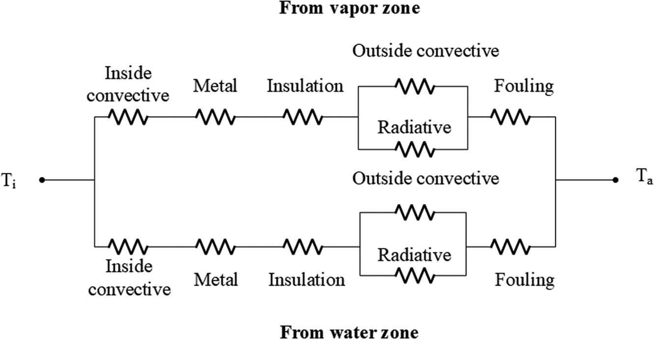
To solve the preceding equation, it is crucial to accurately estimate the heat loss at each time step. As depicted in Figure 3, a thermal resistance network is constructed to illustrate the detailed heat transfer pathways. Heat loss from the water tank primarily occurs through two regions: the liquid surface and the vapor surface. The corresponding heat transfer mechanisms include: (1) thermal conduction through the multilayer tank wall, (2) convective heat exchange between the internal fluid and the inner wall surface, (3) convective heat dissipation from the external shell to the ambient air and (4) thermal radiation emitted from the tank surface to the surrounding environment. These mechanisms collectively determine the overall heat loss rate and are integral to the accuracy of the transient energy balance model.
Thermal resistance of a thermal storage water tank.

Figure 3. Long description
This figure illustrates a thermal resistance network diagram between nodes Ti on the left and Ta on the right. The network splits into two parallel branches. The top branch represents heat transfer from the vapor zone, and the bottom branch represents heat transfer from the water zone. Both branches share an identical series–parallel layout of thermal resistances. Moving from left to right along either branch, heat flows through an ‘Inside convective’ resistance, a ‘Metal’ resistance, and an ‘Insulation’ resistance in series. Following the insulation layer, the path splits into a parallel network consisting of an ‘Outside convective’ resistance on top and a ‘Radiative’ resistance on the bottom. These parallel resistances recombine and connect in series to a final ‘Fouling’ resistance before reaching the node Ta on the far right.
Based on the electrical analogy commonly applied in thermal system modeling, the heat flux is represented as the temperature difference divided by the total thermal resistance, denoted as
$ {\psi}_w $
 for the water region and
$ {\psi}_v $
 for the vapor region. Accordingly, Equations (6) and (7) are formulated to quantify the heat losses from the water and vapor interfaces, respectively.


in this context, T represents temperature, where the subscripts ‘a’ and ‘t’ denote the ambient environment and the tank surface, respectively. The terms
$ {U}_w $
 and
$ {U}_v $
 refer to the overall heat transfer coefficients associated with the water and vapor regions. Correspondingly, the heat losses through the liquid and vapor interfaces are denoted as
$ {\dot{Q}}_{w,l} $
 and
$ {\dot{Q}}_{v,l} $
 , respectively, and are determined using these coefficients along with the temperature gradients.
Notations
$ {A}_w $
 and
$ {A}_v $
 denote the surface areas of the water and vapor phases, respectively. Given the capsule shaped geometry of the tank (as illustrated in Figure 2c), a piecewise function is employed to estimate the dynamic variation of the liquid surface area over time. The corresponding vapor surface area is then determined by subtracting the liquid surface area from the total internal surface area of the tank.


Building upon the series–parallel structure of the thermal resistance network illustrated in Figure 3, the overall thermal resistances associated with the water and vapor surfaces are calculated using Equations (11) and (12), respectively, as outlined in reference (Çengel and Ghajar, Reference Çengel and Ghajar2015). These equations account for the combined effects of conduction, convection and radiation along the respective heat transfer paths.


in these expressions,
$ {k}_s $
 and
$ {k}_i $
 represent the thermal conductivities of the tank’s metallic shell and insulation layer, while
$ {t}_s $
 and
$ {t}_i $
 denote their respective thicknesses. The terms
$ {h}_f $
 and
$ {h}_r $
 correspond to the heat transfer coefficients accounting for fouling and radiative heat exchange. Meanwhile,
$ {h}_i $
 and
$ {h}_a $
 refer to the convective heat transfer coefficients on the inner fluid side and the ambient air side, respectively.
In the water storage system, the capsule shaped is positioned vertically. To characterize the heat transfer between the tank wall and the internal liquid or vapor phases, a set of empirical correlations are employed to estimate the average Nusselt number, as referenced in (Rohsenow et al., Reference Rohsenow, Hartnett and Cho1998; Majumdar et al., Reference Majumdar, Valenzuela, LeClair and Moder2016). Based on these correlations, the internal convective heat transfer coefficient is subsequently determined using the standard definition of the Nusselt number, linking it to thermal conductivity and characteristic length scales.
The basic idea of these thermal correlations is to first derive an equation for the laminar Nusselt number (
$ {Nu}_l $
 ). In the case of laminar flow, the natural convection boundary layer is generally not very thin. Therefore, the laminar Nusselt number can be regarded as a corrected form derived from both the conduction Nusselt number (
$ {Nu}_{cond} $
 ) and the laminar thin-layer Nusselt number (
$ {Nu}^T $
 ). In this context, the conduction Nusselt number refers to the special case where the Rayleigh number approaches zero and there is no fluid motion. Following the laminar formulation, another equation is developed to describe the turbulent Nusselt number (
$ {Nu}_t $
 ), which is based on the assumption that the flow over the surface is in a fully turbulent state. Finally, the average Nusselt number (
$ Nu $
 ) is determined by combining the laminar and turbulent Nusselt numbers into a single expression. This combined correlation provides a unified formulation applicable to all flow regimes on the surface, thereby ensuring its validity for a wide range of practical heat transfer conditions.


where,
$ {\overline{C}}_l $
 $ ({\overline{C}}_l=0.671/{\left(1+{\left(0.492/\mathit{\Pr}\right)}^{9/16}\right)}^{4/9}) $
 and
$ {\overline{C}}_t $
 (as listed in Table 1) are constants that depend on the Prandtl number.
$ D $
 ,
$ G $
 and
$ {k}_l $
 represent the diameter of the tank, a ratio of integrals (as listed in Table 1) and the thermal conductivity of the liquid, respectively. The Rayleigh number (Ra) characterizes the natural convection process occurring within the liquid phase. In addition, the parameters m and n are determined by fitting to experimental data, as shown in Table 1.
Constant parameters used in empirical correlations for a vertical capsule shaped tank (Rohsenow et al., Reference Rohsenow, Hartnett and Cho1998)

Table 1. Long description
The table features a 2D vertical capsule-shaped tank sketch on the left, demonstrating geometric height L and diameter D. To the right of the sketch is a multi-column data matrix. The vertical columns represent the length-to-diameter ratio (L/D), a Nusselt number parameter, geometric constants G and n, a composite header for parameter C_t under four distinct Pr values (Pr = 0.71, 6.0, 100 and 2000) and a constant m. The horizontal rows correspond to four different aspect ratios ranging from two to five. The matrix shows the qualitative variations of these empirical parameters and constants across different length-to-diameter configurations.
In addition, an empirical correlation is employed to evaluate the natural convective heat transfer between the outer surface of the vertically oriented capsule shaped tank and the surrounding ambient air, as reported in previous studies (Bergman, Reference Bergman2011; Joseph et al., Reference Joseph, Agrawal, Agarwal, Pisharady and Sunil Kumar2017). This correlation primarily characterizes the relationship between the external convective heat transfer coefficient, the Prandtl number and the Reynolds number (
$ \mathit{\operatorname{Re}} $
 ).

here,
$ {k}_a $
 denotes the thermal conductivity of the ambient air.
Since the heat losses from the water surface and the vapor surface occur simultaneously and independently, they can be considered as parallel heat transfer paths. In addition, the pipelines connecting the tanks are relatively short. Compared with that from the large surface area of the tanks, heat loss along the pipelines is negligible and is therefore neglected in the model. Thus, the total heat loss
$ {\dot{Q}}_{loss} $
 is calculated as the sum of the heat losses from both interfaces, as expressed in Equation (19).

Mass conservation constitutes a fundamental governing equation crucial for monitoring the changes in both water and vapor masses over each discrete time step. At the subsequent time step, denoted as i + 1, the total mass is determined by summing the water and vapor masses present at time step i, along with the net mass changes of water (
$ {\dot{m}}_w $
 ) and vapor (
$ {\dot{m}}_v $
 ) occurring during the time interval
$ \Delta t $
 , as formulated in Eq. (20).

Considering that the total volume (
$ V $
 ) of the capsule shaped water tank is fixed and does not change, the mass conservation equation can be rewritten by incorporating the relationship between specific volume and mass, which leads to the formulation shown in Eq. (21).

Because both Eqs. (2) and (21) depend on the temperatures at time steps i and i + 1, the temperature at time step i + 1 can be determined using the known temperature at time step i. Following this, the pressure corresponding to the calculated temperature is evaluated by referring to the saturated water property table (Çengel et al., Reference Çengel, Boles and Kanoglu2019).
Furthermore, the capsule shaped tanks connected in series are incorporated into this transient model. In this context, accurately describing the mass flow rate between different tanks becomes crucial during both the charging and discharging processes. Regarding the mass flow within a pipe connecting two capsule-shaped tanks, it can be approximated as a free jet flow, primarily driven by the pressure difference (
$ \Delta P $
 ) between the two ends of the pipe. Consequently, the fluid velocity within the pipe (
$ {V}_c $
 ) can be estimated using the Bernoulli equation, and the resulting mass flow rate (
$ {\dot{m}}_c $
 ) is determined by the product of this velocity and the pipe’s cross-sectional area (
$ {A}_c $
 ), as expressed in Eqs. (22) and (23) (Gerhart et al., Reference Gerhart, Andrew and John2016).


Time step determination
Discretizing the governing equations with respect to time is essential for solving the dynamic model effectively. The chosen size of the time step has a direct impact on both the accuracy and stability of the model. However, selecting excessively small-time steps can lead to a substantial increase in computational cost and time. Therefore, this study investigates a balance between computational efficiency and accuracy by testing four different time step sizes (50 s, 10 s, 5 s and 2 s) using a model of 2 tanks divided into 12 blocks. The model’s performance was assessed by analyzing the temporal profiles of time, temperature and water level throughout the charging and discharging processes.
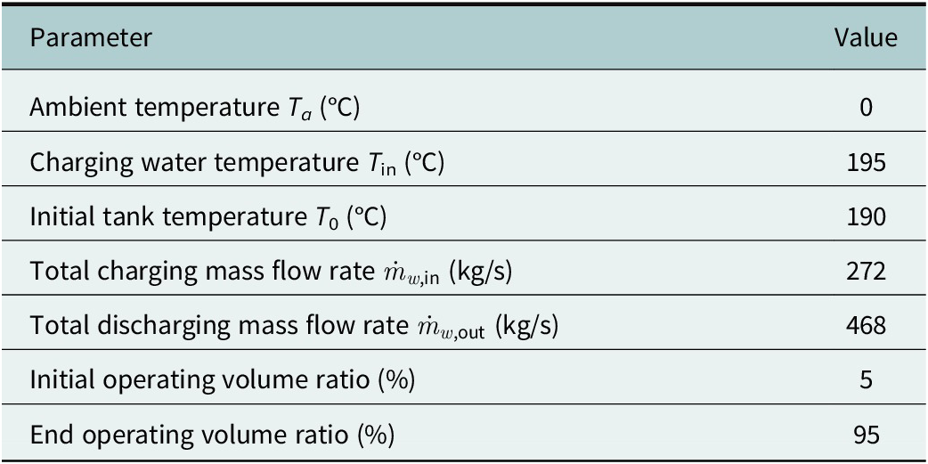
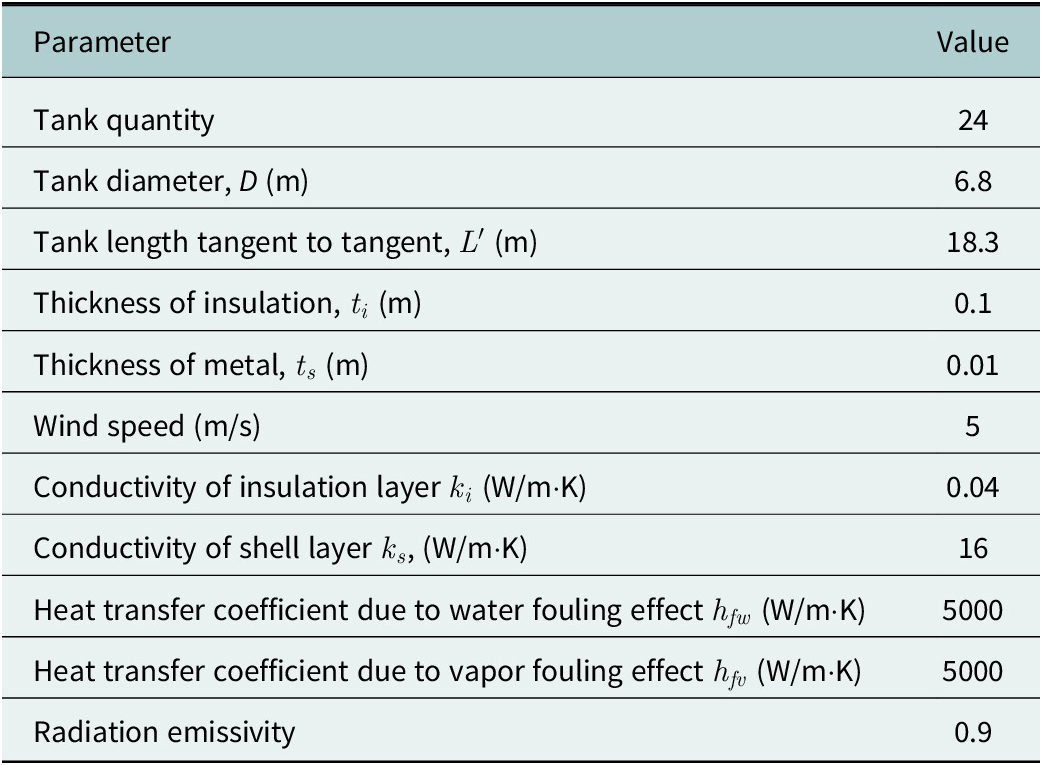
Additionally, in order to comprehensively assess the thermal performance of the capsule-shaped water tanks within the transient model framework, it is essential to define the relevant physical and geometric input parameters. For this study, a project based in Australia was selected, with key operating and design parameters provided by HYDROSTOR Inc., a CAES system operator. The water tank system considered here is a subsystem of the overall CAES system. Accordingly, several operating parameters, including the inlet and outlet water temperatures and the mass flow rate, were determined based on the requirements for cooling and reheating compressed air during the CAES process. In addition, the system was designed to meet engineering requirements, specifically that the charging process lasts no less than 13 hours and the discharging process no less than 8 hours. These parameters are presented in detail in Tables 2 and 3. Besides, this project is currently at the preliminary design stage. To enable the simulations, the pipeline diameters in both the water and gas zones were set to 10 cm in this study, based on Hydrostor’s initial reference design (Hydrostor, 2025).
Physical parameters in the thermodynamic model (Hydrostor, 2025)

Table 2. Long description
This table consists of a simple two-column data layout. The first column lists various thermodynamic input parameters, including ambient temperature, charging water temperature, initial tank temperature, total mass flow rates for both charging and discharging processes, as well as initial and end operating volume ratios. The second column presents the specified constant values or ratios assigned to each corresponding parameter for the model evaluation.
Initial designing parameters for two thermal storage schemes (Hydrostor, 2025)

Table 3. Long description
This table consists of a simple two-column data layout. The first column lists various initial design parameters for the two thermal storage schemes, including tank quantity, geometric dimensions such as diameter and tangent-to-tangent length, thicknesses of insulation and metal layers, wind speed, thermal conductivities of insulation and shell layers, heat transfer coefficients related to water and vapor fouling effects, and radiation emissivity. The second column presents the specific constant numerical values or ratios assigned to each corresponding design parameter.
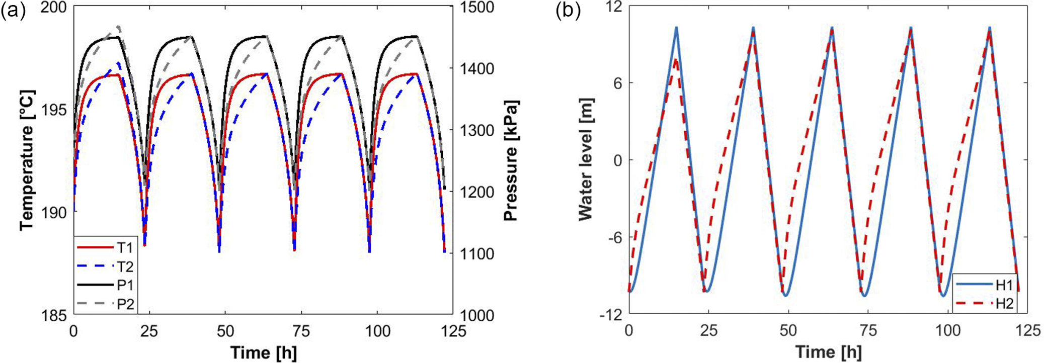
Figure 4 illustrates the variations in temperature and water level during five charging–discharging cycles using a time step of 5 seconds for the two-tank model without a gas-zone connection. The results show that after the second cycle, the variations of these thermofluidic parameters tend to stabilize, and no significant cumulative or drift effects are observed. Therefore, to reduce computational cost, only the first three cycles are discussed in the subsequent analysis.
Thermofluidic performances of a 2-tank system without a gas-zone connection under five cycles: (a) temperature variations and (b) water-level variations. T, P and H denote temperature, pressure and water level, respectively.

Figure 4. Long description
This figure group consists of two line graphs, (a) and (b), illustrating the thermofluidic performances of a 2-tank water tank system without a gas-zone connection under five charging-discharging cycles over a duration of 125 hours. Graph (a) plots temperature variations on the left vertical axis (ranging from 185 to 200 degrees Celsius) and pressure variations on the right vertical axis (ranging from 1000 to 1500 kPa) against time on the horizontal axis. It shows fluctuating cyclical profiles for temperatures T1, T2 and pressures P1, P2. Graph (b) plots water level variations on the vertical axis (ranging from −12 to 12 m) against time, showcasing oscillating cyclical waves for water levels H1 and H2. In both graphs, the variations tend to stabilize after the second cycle, with the subsequent cycles showing highly consistent periodic behavior.
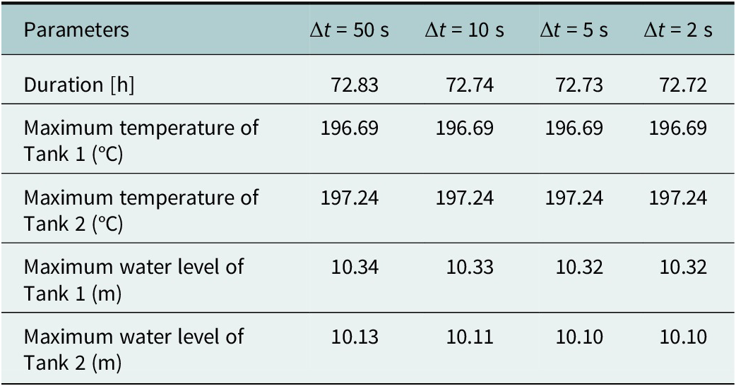
As presented in Table 4, the primary performance metrics for the two-tank model without a gas zone connection were assessed under various time step sizes. It was observed that when the time steps were shorter than 50 seconds, the model outputs – such as operation durations, temperature profiles and water-level variations throughout the three stages – remained consistently stable and showed minimal variation.
Effect of time step on the dynamic two-tank model without a gas-zone connection

Table 4. Long description
This table presents a multi-column data layout evaluating sensitivity to temporal resolution. The first column lists several output performance parameters, including total duration, maximum temperatures for both Tank 1 and Tank 2, as well as maximum water levels for both Tank 1 and Tank 2. The subsequent four columns represent different time step scenarios decreasing in size. The horizontal matrix qualitative demonstrates how these dynamic thermofluidic maximums and durations respond and converge as the simulation time step becomes smaller.
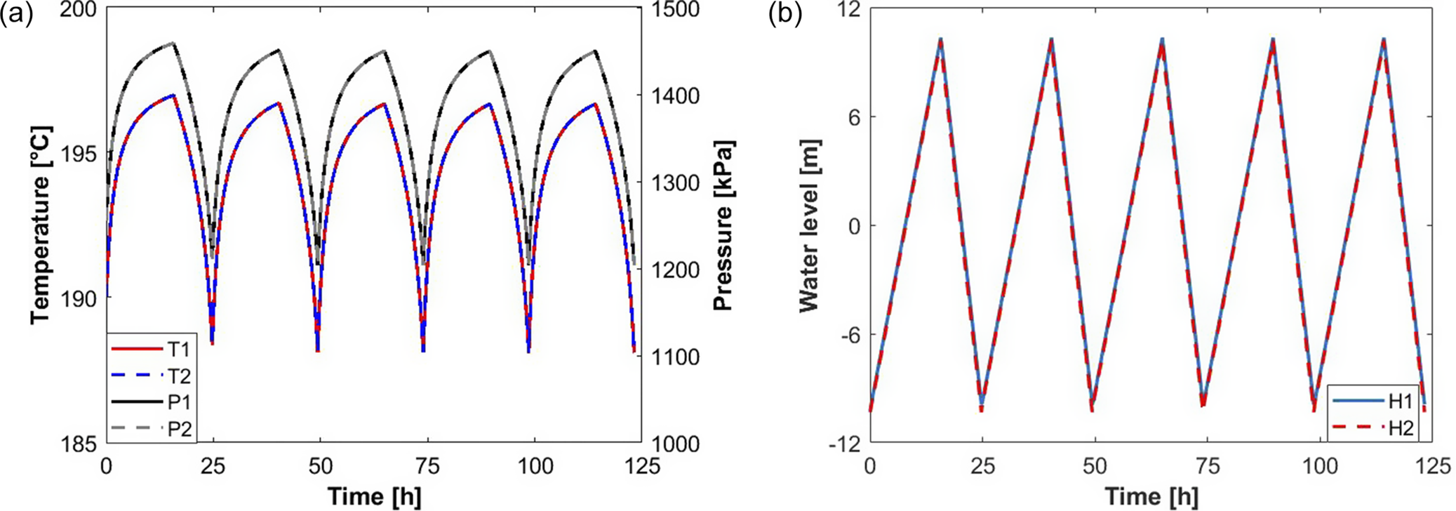
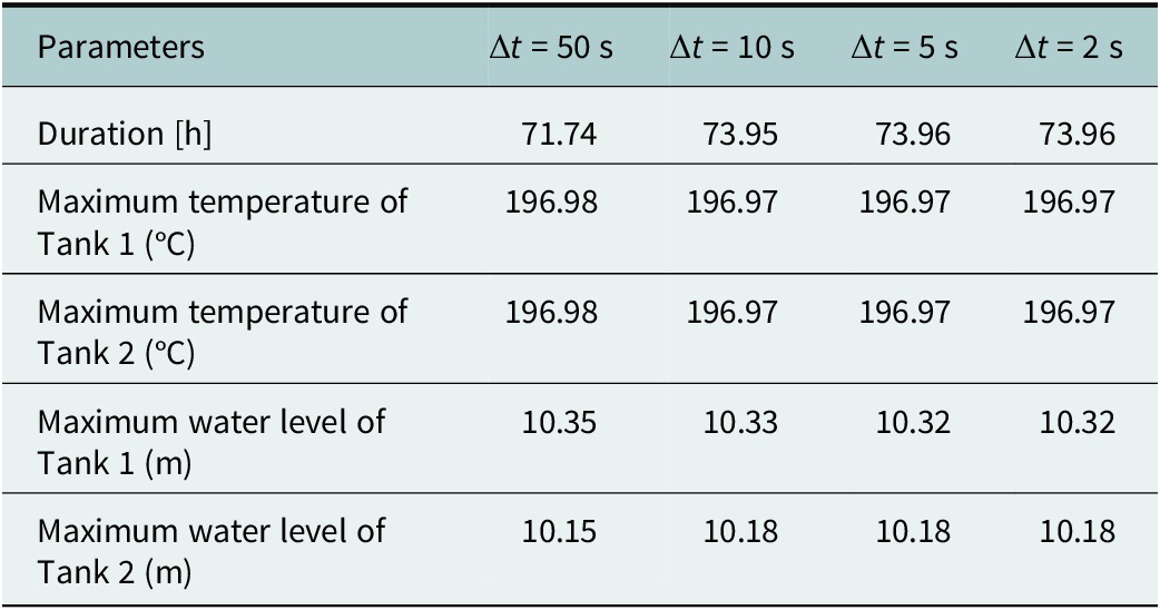
Similarly, based on the results in Figure 5, the first three cycles were discussed for the model with a gas zone in the following studies. Table 5 presents a summary of the corresponding results for the two-tank model that includes a connected gas zone. Due to the inclusion of the gas-zone connection, this configuration demonstrates more pronounced dynamic behavior compared to the previous model without the gas zone. Nevertheless, the model responses become stable when the time step is chosen to be less than 5 seconds. Therefore, a consistent time step of 5 seconds is adopted for all subsequent simulations to guarantee both accuracy and numerical stability across both types of models.
Thermofluidic performances of a 2-tank system with a gas-zone connection under five cycles: (a) temperature and (b) water level.

Figure 5. Long description
This figure group consists of two line graphs, (a) and (b), illustrating the thermofluidic performances of a 2-tank water tank system with a gas-zone connection under five charging-discharging cycles over 125 hours. Graph (a) plots temperature variations on the left vertical axis (185 to 200 degrees Celsius) and pressure variations on the right vertical axis (1000 to 1500 kPa) against time on the horizontal axis. It displays periodic fluctuations for temperatures T1, T2 and pressures P1, P2. Graph (b) plots water level variations on the vertical axis (-12 to 12 meters) against time, showing the cyclical oscillating profiles for water levels H1 and H2. Similar to Figure 4, the variations tend to stabilize after the second cycle, with the subsequent cycles showing highly consistent periodic behavior.
Effect of time step on the dynamic two-tank model with a gas-zone connection

Table 5. Long description
This table presents a multi-column data layout evaluating sensitivity to temporal resolution. The first column lists several output performance parameters, including total duration, maximum temperatures for both Tank 1 and Tank 2, as well as maximum water levels for both Tank 1 and Tank 2. The subsequent four columns represent different time step scenarios decreasing in size. The horizontal matrix qualitatively demonstrates how these dynamic thermofluidic maximums and durations respond and converge for the gas-zone connected system as the simulation time step becomes smaller.
Pressure loss in the connected pipe
Based on the total mass flow rates during the charging and discharging processes, the corresponding mass flow rates for each tank are approximately 11.3 kg/s during charging and 19.5 kg/s during discharging, calculated by dividing the total mass flow rate by the number of tanks. Considering the pipe diameters (8 cm, 10 cm and 12 cm) examined in this study, the water flow in the pipelines remains in a turbulent regime under the present operating conditions, as their Reynolds numbers reach on the order of
$ {10}^5 $
 . Therefore, it is necessary to examine whether pressure losses in the pipelines have a noticeable impact on the model results.
When pressure losses in the pipelines are considered, the velocity equation (Eq. (22)) can be rewritten as Eq. (24). The pressure loss (
$ {P}_{loss} $
 ) is calculated using Eq. (25). In addition, the friction factor (
$ f $
 ) is determined using the Haaland equation (Gerhart et al., Reference Gerhart, Andrew and John2016), as expressed in Eq. (26).


where
$ d $
 and
$ l $
 are the diameter and length of the pipeline, respectively. The head loss in the pipe is denoted as
$ {h}_l $
 . The pipe roughness is represented by
$ \varepsilon $
 , with a value of
$ 4.572\times {10}^{-5}\;\mathrm{m} $
 provided by Hydrostor (2025). In addition, the velocity (
$ {V}_c $
 ) can be obtained by simultaneously solving Eqs. (22)–(24) using a gradient descent method.
Based on Eq. (25), the pressure loss is strongly related to the pipeline length-to-diameter ratio (
$ L/D $
 ), in addition to the flow regime. Therefore, to evaluate the effect of pressure loss on the simulation results, a parametric analysis was performed using the two-tank model without gas-zone connection by varying the pipeline length while maintaining a constant diameter of 10 cm. The results (as shown Figure 6) indicate that the effect of pressure loss on the simulation results becomes non-negligible when the pipeline length-to-diameter ratio (
$ L/D $
 ) reaches approximately 100. In the present study, such long pipelines are typically not used to connect tanks within the same block. Therefore, pressure losses are neglected in the subsequent analysis to reduce computational resources.
Effects of pressure loss on the temperatures of the two-tank model with a gas-zone connection: (a) Tank 1 temperature (diameter = 10 cm) and (b) Tank 2 temperature (diameter = 10 cm).

Figure 6. Long description
This figure group consists of two line graphs, (a) and (b), illustrating the effects of pressure loss on the temperatures of a 2-tank model with a gas-zone connection under four different scenarios over three full cycles (around 75 hours). Graph (a) shows the temperature profile of Tank 1, and graph (b) shows the temperature profile of Tank 2. In both graphs, the vertical axis represents temperature ranging from 185 to 200 degrees Celsius, and the horizontal axis represents time from 0 to 75 hours. Four curves are plotted in each graph, comparing a baseline case with no pressure loss against three different pipeline lengths: l = 1 m, l = 5 m and l = 10 m, while maintaining a constant pipeline diameter of 10 cm. The curves overlap significantly during the first cycle, but a noticeable divergence occurs during the second and third cycles, where longer pipeline lengths result in a visible drift or variation in peak temperatures.
Comparison of the two tank layouts
The primary motivation behind this design approach is to reduce the construction cost of the water storage subsystem by segmenting the overall tank system into multiple independent modules. Within each module, it is anticipated that the water tanks can share a unified set of auxiliary components – such as sensors, valves and piping systems. To enable the feasibility of this shared configuration, it is crucial to ensure that key thermofluidic parameters – including temperature, pressure and water level – exhibit highly synchronized variations across all tanks within the same module.
In this section, two distinct layout configurations are proposed, both employing a cascade connection strategy within each tank block. The primary distinction between the two lies in whether the gas zones of adjacent tanks are interconnected. For a representative case involving a block composed of two tanks, a comparative analysis is conducted to evaluate the synchronization of thermofluidic performance variations between the two configurations. This evaluation is carried out in detail using the transient model developed in the preceding section.
Thermofluidic performances of the two-tank without gas zone connection
In this layout scheme, a pipeline with an inner diameter of 10 cm is used to connect the bottom water zones of the two tanks, enabling free water flow driven by the pressure difference between them. During the charging stage, water at a constant temperature of 195 °C is introduced into Tank 1. Assuming a total of 12 blocks, each consisting of two interconnected tanks (as shown in Figure 2), the total mass flow rate during the charging process is 22.66 kg/s. Simultaneously, due to the existence of the interconnecting pipeline, water stored in Tank 1 can supplement the water in Tank 2. The charging process concludes when the water level in Tank 1 reaches its upper operating limit, corresponding to the specified end operating volume ratio. During the discharging stage, water is released through the outlet of Tank 2 at a mass flow rate of 40.5 kg/s. Again, due to the pressure differential and the interconnection between the tanks, water from Tank 1 can be transferred into Tank 2 to sustain the outflow. The discharging process terminates when the water level in Tank 2 drops below the initial operating volume ratio. The temporal variations of the associated thermofluidic parameters, including temperature, pressure and water level, under this configuration are illustrated in Figure 7.
Thermofluidic performances of a 2-tank system without a gas-zone connection: (a) temperature and pressure variations and (b) water-level variations.

Figure 7. Long description
This figure group consists of two line graphs, (a) and (b), illustrating the thermofluidic performances of a 2-tank water tank system without a gas-zone connection over three cycles (around 75 hours). Graph (a) plots temperature variations on the left vertical axis (185 to 200 degrees Celsius) and pressure variations on the right vertical axis (1000 to 1500 kPa) against time on the horizontal axis, showcasing cyclical fluctuations for temperatures T1, T2 and pressures P1, P2 with a noticeable time-lag effect between the two tanks. Graph (b) plots water level variations on the vertical axis (-12 to 12 meters) against time, showing asynchronous cyclical profiles for water levels H1 and H2. In both graphs, the variations stabilize and exhibit a highly regular periodic pattern after the second cycle.
The results demonstrate that the thermofluidic performance in both tanks undergoes dynamic variations from the initial condition, primarily due to the alternating processes of water filling and draining. After two complete operational cycles, these variations gradually tend to stabilize and exhibit a more regular pattern. As illustrated in Figure 7a, a distinct delay in the temperature response is observed between the two tanks. Specifically, during the charging phase, the inlet water for Tank 2 is supplied from Tank 1. Unlike Tank 1, which directly receives water at a constant temperature of 195 °C, the temperature of the water entering Tank 2 is subject to fluctuations, depending on the thermal state of the water stored in Tank 1. As a result, Tank 2 exhibits a delayed temperature response. Correspondingly, the saturated pressure inside each tank – being closely linked to the water temperature – also exhibits similar lagging behavior. Since the gas zones of the two tanks are not interconnected, their pressure variations evolve independently, even though they follow broadly similar trends.
In addition to the time-lag effects observed in temperature and pressure, the water-level fluctuations between the two tanks also exhibit asynchronous behavior, as shown in Figure 7b. This lack of synchronization is primarily caused by the differences in the mass flow rates during the filling and draining processes of the two tanks. According to the operating logic of the system, the inflow rate into Tank 1 and the outflow rate from Tank 2 are maintained constant. In contrast, the inflow rate into Tank 2 and the outflow rate from Tank 1 are not fixed, but vary over time. These variable flow rates are primarily determined by the dynamic differences in water level and saturated pressure between the two tanks, as further depicted in Figure 8.
Variation of water mass flow rate in the connecting pipe between the two water tanks.

Figure 8. Long description
This figure is a single line graph plotting the water mass flow rate against time, spanning three complete operational cycles. The curve exhibits a highly periodic and dynamic cyclical wave profile. At the beginning of each cycle, the flow rate undergoes a rapid and sharp spike to its maximum peak, followed immediately by a steep decline until it reaches a low-level plateau. Midway through each cycle, the flow rate experiences another sudden increase to form a secondary, elevated plateau where it remains stable before dropping back down. This entire fluctuating pattern of sharp peaks, deep valleys, and stable plateaus repeats with high consistency across all three cycles.
Thermofluidic performances of the two-tank system with a gas-zone connection
In an alternative layout scheme, an additional pipeline with an inner diameter of 10 cm is introduced to connect the gas zones of the two tanks. This gas zone interconnection enables vapor to flow between the tanks, with the direction of flow determined by the pressure difference between the respective gas zones. Following the same operating logic as applied in the previous layout, the subsequent analysis investigates the thermofluidic behavior of the two-tank system incorporating the gas zone connection. The evaluation is conducted over three complete charging–discharging cycles to capture the system’s dynamic response and stabilization trends. The corresponding results, including variations in temperature, pressure and water level, are illustrated and analyzed in detail in Figure 9.
Thermofluidic performances of a 2-tank system with a gas-zone connection: (a) temperature and pressure variations and (b) water-level variations.

Figure 9. Long description
This figure group consists of two line graphs, (a) and (b), illustrating the thermofluidic performances of a 2-tank water tank system with a gas-zone connection over three full operational cycles. Graph (a) plots temperature and pressure variations against time, showing highly consistent, overlapping, and synchronized periodic fluctuations for the parameters across both tanks. Graph (b) plots water level variations against time, displaying identical and overlapping triangular wave oscillations for both tanks. Throughout all cycles, the thermofluidic variations exhibit high symmetry and exceptional stability right from the initial cycle, with no visible time-lag or asynchronous behavior between the two tanks.
Similar to the behavior observed in the two-tank system without a gas-zone connection, the thermofluidic performance variations – including temperature, pressure and water level – tend to stabilize after two complete charging and discharging cycles. However, as depicted in Figure 9a, the delays in temperature and pressure responses between the two tanks are significantly reduced. This observation confirms that the presence of the gas-zone connector plays a critical role in promoting more synchronized thermofluidic behavior across the tanks. By enabling unrestricted vapor exchange, the connector effectively facilitates the equalization of pressure and temperature throughout both charging and discharging stages, thereby enhancing the dynamic coupling of the system.
Except to the improved synchronization of temperature and pressure, the water levels in both tanks also remain nearly identical throughout the operational period, as illustrated in Figure 9b. As shown in Figure 10a, vapor is able to flow freely between the tanks via the connecting pipeline, contributing to the continuous balance of saturated pressure. Consequently, unlike the configuration without a gas-zone connection, the water mass flow rates into Tank 2 and out of Tank 1 are now primarily governed by the difference in water levels between the tanks. Furthermore, Figure 10b demonstrates that the net water mass flow rates in both tanks tend to converge over time, indicating increasingly stable flow dynamics. As a result, the water-level variations in the two tanks become progressively more synchronized.
Variations of vapor and water mass flow rate between the two water tanks: (a) vapor mass flow rate and (b) water mass flow rate.

Figure 10. Long description
This figure group consists of two line graphs, (a) and (b), illustrating the mass flow rates between two water tanks with a gas-zone connection over three full operational cycles. Graph (a) plots the vapor mass flow rate against time, which exhibits a highly symmetrical and periodic high-frequency oscillation forming a fluctuating envelope wave pattern, supplemented by an inset zoom-in view showing rapid periodic micro-oscillations. Graph (b) plots the water mass flow rate against time, showcasing a step-like cyclical waveform with sharp spikes at the beginning of each cycle that gradually damp down and converge, indicating increasingly stable fluid dynamics over time.
Overall, when a multi-tank design does not include a gas zone connection, the temperature, pressure and water-level variations among different tanks, including the end tanks, exhibit significant differences. After connecting the gas zone, these differences are substantially reduced, leading to more consistent thermofluidic performance changes throughout the tanks. Therefore, incorporating a gas-zone connection is necessary in a multi-tank design.
Sensitivity studies of multi-tank with gas-zone connections design
The findings discussed in the preceding section have confirmed that incorporating gas connections is essential for ensuring effective thermofluidic performance in multi-tank configurations. However, to further reduce the overall construction costs of the thermal storage system, it is generally preferable to maximize the number of interconnected tanks arranged in a cascade layout within each block. Accordingly, this section investigates three distinct multi-tank design configurations: 12 blocks with 2 tanks per block, 8 blocks with 3 tanks per block and 6 blocks with 4 tanks per block.
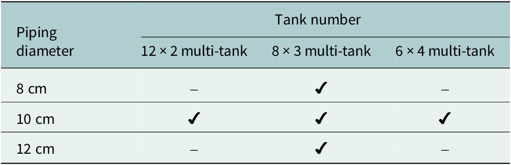
In evaluating these configurations, the degree of synchronization in the variations of thermofluidic parameters – such as temperature, pressure and water level – is considered a primary metric for assessing the practicality and performance of each design. Among the various design parameters, the diameter of the interconnecting pipelines plays a critical role in governing the flow dynamics and the thermal and pressure equilibrium among tanks within a single block. To systematically examine this influence, three different pipeline diameters are analyzed in the following studies. These analyses aim to elucidate the impact of connection size on system responsiveness, coordination among tanks and the overall feasibility of larger-scale multi-tank integration. Table 6 indicates the test matrix for the sensitivity studies.
Test matrix of the sensitivity studies

Table 6. Long description
This table presents a sensitivity test matrix with a diagonal-split top-left header for piping diameter and tank number. The horizontal header lists three multi-tank configurations based on tank numbers, while the vertical first column lists three different pipeline diameters. Within the data grid, checkmarks indicate selected simulation scenarios, mapping specific pipe diameters to their corresponding tank configurations, while hyphens represent excluded combinations. It qualitatively defines which experimental parameters are combined and tested across the different case studies.
Effect of tank quantity on thermofluidic performances in a multi-tank design
In all three multi-tank configurations, the diameters of the pipelines connecting both the water and gas zones are uniformly set to 10 cm. During the charging phase, hot water at a temperature of 195 °C is introduced into the first tank in each block, while during the discharging phase, water is extracted from the last tank. To ensure consistency in the total mass flow rate of water entering and exiting the system, the charging and discharging mass flow rates per block are adjusted according to the specific design configurations: 22.66–39 kg/s for the 12 × 2-tank setup, 34–58.5 kg/s for the 8 × 3-tank setup and 45.33–78 kg/s for the 6 × 4-tank setup. These rates are selected to achieve comparable system-level throughput (total mass flow rates: 468 kg/s [discharging] and 272 kg/s [charging]) across the different arrangements. The corresponding variations in temperature and pressure for the three multi-tank configurations over three complete charging–discharging cycles are presented in Figure 11, forming the basis for assessing pressure and temperature synchronization among the different designs.
Variations of temperature and pressure in the three different multi-tank designs: (a) 12 × 2-tank, (b) 8 × 3-tank and (c) 6 × 4-tank.

Figure 11. Long description
Three line graphs labeled a, b, and c share identical axes. The horizontal x-axis represents Time in h from 0 to 75. The primary vertical y-axis on the left represents Temperature in degrees Celsius from 185 to 200. The secondary vertical y-axis on the right represents Pressure in k P a from 1000 to 1500.
* Panel a: Displays four lines. T 1 (solid red) and T 2 (dashed blue) track together, showing three cycles of rapid increase followed by a sharp drop, peaking near 197 degrees Celsius. P 1 (solid black) and P 2 (dashed grey) track together at a higher amplitude, peaking near 1450 k P a.
* Panel b: Displays six lines. T 1, T 2, and T 3 (dotted green) overlap perfectly. P 1, P 2, and P 3 (dotted magenta) also overlap perfectly. The trends follow the same cyclic pattern as panel a, with temperature peaking at 197 and pressure peaking at 1450.
* Panel c: Displays eight lines. T 1 through T 4 and P 1 through P 4 are plotted. All temperature lines (T) are perfectly coincident, and all pressure lines (P) are perfectly coincident. The time scale on the x-axis for this panel ends at 60 h, showing two and a half cycles compared to the three cycles in panels a and b.
Similar thermofluidic performance patterns are observed across the three multi-tank configurations. Specifically, the temperature and pressure variations within each tank stabilize after two complete operating cycles. Furthermore, within each block, the tanks exhibit nearly identical temperature and pressure profiles across all three designs. Since the steam regions are connected, the vapor pressure tends to equalize among the tanks; therefore, increasing the number of tanks within a block would not obviously affect the synchronization of temperature and pressure variations. These findings confirm that the implementation of gas zone connectors effectively balances the pressures and temperatures among tanks in all configurations. However, differences emerge in the water-level variation trends among tanks within a block, as illustrated in Figure 12. As the number of tanks connected in series increases within a block, the synchronization of water-level fluctuations among the tanks decreases markedly. When the pipeline diameter is fixed, the hydraulic exchange capacity among the tanks is limited. As the number of tanks connected in series increases, the difference in inflow and outflow responses between upstream and downstream tanks becomes more pronounced. Consequently, the synchronization of water-level variations decreases as the number of tanks per block increases.
Variations of water level in the three different multi-tank designs: (a) 12 × 2-tank, (b) 8 × 3-tank and (c) 6 × 4-tank.

Figure 12. Long description
The figure consists of three panels labeled a, b, and c. All panels share the same axes: the X-axis represents Time in h from 0 to 75, and the Y-axis represents Water level in m from -12 to 12.
* Panel a: Contains two lines, H 1 (solid blue) and H 2 (dashed red). Both lines follow an identical triangular wave pattern, oscillating between approximately -10 and 10 meters with three complete peaks at 15, 40, and 65 hours.
* Panel b: Contains three lines, H 1 (solid blue), H 2 (dashed red), and H 3 (dashed orange). H 1 and H 2 are nearly identical. H 3 follows the same triangular frequency but shows slightly lower troughs, reaching approximately -11 meters compared to the -10 meters of H 1 and H 2.
* Panel c: Contains four lines, H 1 (solid blue), H 2 (dashed red), H 3 (dashed orange), and H 4 (dashed purple). The lines show increasing divergence at the troughs. H 1 has the highest troughs at -4 meters, while H 4 has the deepest troughs, returning to the baseline of -10 meters. All four variables maintain synchronized peaks at approximately 10 meters.
Effect of water flow rate on water-level variations in a multi-tank design
In principle, connecting more tanks in series is desirable for multi-tank configurations. However, as shown in Figure 12, increasing the number of tanks also increases the hydraulic resistance in the pipelines, making an obvious gap in the water level within different tanks gradually. To further enhance the synchronization of water-level variations among tanks, a direct method is to adjust water mass flow in and out of the system. To this end, the performance of the 8 × 3 configuration was evaluated under three different water mass flow rates: a reduced flow rate corresponding to that of the 12 × 2 configuration, its original flow rate and an increased flow rate corresponding to that of the 6 × 4 configuration. The results are displayed in Figure 13.
Variations in the water level under three different water mass flow rates: (a) reduced flow rate, (b) original flow rate and (c) increased flow rate.

Figure 13. Long description
The figure consists of three panels, each with a y-axis representing Water level in meters ranging from -12 to 12 and an x-axis representing Time in hours. Each panel contains three data series: H 1 (solid blue line), H 2 (dashed red line), and H 3 (dashed orange line).
* Panel a: The x-axis ranges from 0 to 110 hours. The three lines are nearly perfectly overlapped, showing a periodic triangular wave pattern. The peaks reach approximately 10 meters at 24, 60, and 96 hours, while troughs drop to -10 meters at 0, 36, 72, and 108 hours.
* Panel b: The x-axis ranges from 0 to 75 hours. The triangular wave frequency is higher than in panel a. H 1, H 2, and H 3 show slight divergence at the peaks and troughs. Peaks occur at approximately 15, 38, and 61 hours. H 1 reaches the highest peaks and shallowest troughs, while H 3 shows the greatest negative displacement at the troughs.
* Panel c: The x-axis ranges from 0 to 50 hours. This panel shows the highest frequency and the most significant divergence between the three series. Peaks occur at approximately 11, 27, and 43 hours. H 1 (solid blue) consistently maintains the highest peaks and highest troughs. H 2 (dashed red) is intermediate. H 3 (dashed orange) shows the lowest peaks and the deepest troughs, reaching nearly -11 meters.
The results indicate that reducing the mass flow rate can significantly improve the synchronization of water levels among different tanks within a block. However, the water mass flow rate is typically constrained by the overall design requirements of the CAES system. This implies that, within this project, the flow rate of the water tank system is not freely adjustable.
Effect of piping diameter on water-level variations in a multi-tank design
To enhance the synchronization of water-level variations among tanks while satisfying the specific design requirements of a CAES system, it is necessary to reduce flow resistance by appropriately increasing the diameter of the connecting pipelines. Under the current calculated conditions, the 8 × 3 configuration represents a balanced design, demonstrating the advantages of a multi-tank arrangement while avoiding the need for excessively large pipeline diameters. Therefore, using this configuration as an example, three pipe diameters – 8 cm, 10 cm and 12 cm – are evaluated in the following study. All other operating parameters remain unchanged, with the mass flow rate of the input hot water (at 195 °C) fixed at 34 kg/s and the output water mass flow rate set at 58.5 kg/s. Figure 14 presents the water-level variations recorded over three complete charging–discharging cycles for each of the tested pipe diameters, allowing a direct comparison of their impact on system performance.
Variations of water level under three kinds of diameters of connection pipe: (a) 8 cm, (b) 10 cm and (c) 12 cm.

Figure 14. Long description
A three-panel line graph series labeled a, b, and c. All panels share the same axes. The x-axis is Time in h (hours) ranging from 0 to 75. The y-axis is Water level in m (meters) ranging from -12 to 12. Each graph contains three data series: a solid blue line (H 1), a thick dashed red line (H 2), and a thin dashed orange line (H 3). All series follow a periodic triangular wave pattern with peaks at approximately 15, 35, and 55 hours.
* Panel a: The three lines show significant divergence. H 1 reaches the highest peaks (approx. 10) and shallowest troughs (approx. -5). H 3 shows the deepest troughs (approx. -10) and lowest peaks (approx. 8). H 2 sits between them.
* Panel b: The lines are closer together than in panel a. The peaks and troughs of H 2 and H 3 have shifted closer to the values of H 1, though H 3 still shows slightly deeper troughs.
* Panel c: The three lines H 1, H 2, and H 3 are nearly perfectly overlapped, appearing as a single triangular wave oscillating between approximately -10 and 10 meters.
Reduced flow resistance can be effectively achieved by using larger-diameter connection pipes. As the diameter of the piping increases, the variations in water level among the three tanks exhibit greater consistency and synchronization. This trend indicates that enlarging the pipe diameter is a viable and efficient strategy to enhance the coordination of water-level fluctuations across multiple tanks. Improved uniformity in water-level response not only promotes better thermofluidic performance but also contributes significantly to the overall operational stability and reliability of the system.
Applicability of the multi-tank model under different operating conditions
The model is developed based on fundamental principles of engineering thermodynamics. In theory, it can also be applied to evaluate the thermofluid performance of multi-tank designs under different operating conditions. To verify this, operating parameters from another project by Hydrostor Inc. (Hydrostor, 2025) are adopted to examine the generality of the model. In this case, the ambient temperature is 20 °C, the initial temperature is 185 °C and the inlet water temperature is 198 °C. The 3-tank model with gas zone connections is considered as an example. Figure 15 illustrates the thermofluid performance under these operating conditions, including variations in temperature, pressure and water level. The results show that the multi-tank design still maintains good synchronization in thermofluid behavior under these conditions. Therefore, it is expected that, under different operating conditions, incorporating the gas zone connection remains an effective approach to improve the synchronization of thermofluid performance in multi-tank systems.
Thermofluidic performances of a 3-tank system with gas-zone connections under different operating conditions: (a) temperature and pressure variations and (b) water-level variations.

Figure 15. Long description
This figure group consists of two line graphs, (a) and (b), illustrating the thermofluidic performances of a 3-tank water tank system with gas-zone connections under different operating conditions over three full operational cycles. Graph (a) plots temperature and pressure variations against time, demonstrating highly synchronized, overlapping, and consistent periodic cyclical fluctuations for both temperature and pressure parameters across the multiple tanks. Graph (b) plots water level variations against time, displaying highly uniform and synchronized triangular wave oscillations for the water levels of all three tanks. Throughout the operating period, all thermofluidic parameters exhibit a stable, highly coordinated, and repeatable cyclical behavior across the cycles.
Conclusions
This study proposes a novel multi-tank layout configuration aimed at reducing the construction costs associated with large-scale water storage tanks in a CAES system. To assess the synchronization of thermofluidic performance variations among the tanks, an equilibrium thermodynamic model was developed. Using a configuration composed of 12 blocks with 2 tanks per block, simulation results confirmed that unequal pressure distribution among different tanks is considered the main cause of synchronization loss. To maintain synchronization, the gas regions of the tanks need to be connected, which helps balance the steam pressure among them. This feature plays a crucial role in ensuring synchronized changes in temperature, pressure and water level across the tanks during both charging and discharging operations. Additionally, sensitivity analyses demonstrated that the synchronization of water-level variations progressively degrades as more tanks are connected within a single block. Consequently, for block configurations with more than three tanks, a connection pipe diameter of 10 cm proves insufficient. In such cases, increasing the pipe diameter becomes necessary to effectively reduce flow resistance between tanks and improve the synchronization of water-level variations throughout the system.
Since the project is still at an early stage, this study has several limitations that should be addressed in future research. First, the modelling results indicate that connecting the gas zones can improve thermofluidic synchronization among tanks during the charging and discharging processes. However, these findings should be further verified through experimental studies.
Besides, the equilibrium thermodynamic model used in this work assumes a uniform thermodynamic state within each tank and neglects temperature stratification during the dynamic charging and discharging processes. In practice, physical phenomena such as thermal stratification, flow dynamics and thermal inertia may develop inside the tanks, resulting in spatial variations in temperature and thermophysical properties. Moreover, differences caused by these non-equilibrium phenomena among multiple tanks may lead to inconsistent variations in thermofluidic parameters, which could influence the synchronization behavior during operation. Therefore, the development of a non-equilibrium model is necessary to further evaluate synchronization characteristics in different multi-tank configurations.
In addition, the geometry and diameter of the pipelines connecting the liquid and gas zones may play an important role in the synchronization behavior among tanks, while also affecting the system cost, especially for large-scale multi-tank systems. Determining the optimal number of tanks within a block and the corresponding pipeline parameters may therefore become a multi-criteria decision-making problem, which may require the development of dedicated optimization algorithms. As the project progresses, it will also be necessary to consider additional practical engineering factors to further refine the system design, including structural constraints, safety considerations, site-specific conditions and flow control strategies, which may limit the applicability of the proposed concept at a utility scale.
Nomenclature
-
$ {A}_v $

-
Vapor surface
-
$ {A}_w $
-
Water surface
- CAES
-
Compressed air energy storage
-
$ {\overline{C}}_l $
-
Function of Prandtl number
-
$ {\overline{C}}_t $
-
Empirical correlation constant
- D
-
Diameter of a water tank
- d
-
Diameter of a connected pipe
- f
-
Friction factor
- G
-
Ratio of integrals
-
$ {h}_a $
-
Outside convective heat transfer coefficient
-
$ {h}_f $
-
Heat transfer coefficient due to fouling effect
-
$ {h}_i $
-
Inside convective heat transfer coefficient
-
$ {h}_l $
-
Head loss in the pipe
-
$ {h}_{rw/v} $
-
Heat transfer coefficient due to radiation
-
$ {h}_{v, in} $
-
Enthalpy of input vapor
-
$ {h}_{v, out} $
-
Enthalpy of output vapor
-
$ {h}_{w, in} $
-
Enthalpy of input water
-
$ {h}_{w, out} $
-
Enthalpy of output water
-
$ {k}_i $
-
Conductivity of the insulation layer
-
$ {k}_l $
-
Conductivity of liquid
-
$ {k}_s $
-
Conductivity of the shell layer
-
$ L $
-
Tank length
-
$ l $
-
Pipeline length
-
$ {L}^{\prime } $
-
Tank length tangent to tangent
- m
-
Fitted parameter in overall Nusselt number equation
-
$ {\dot{m}}_{v, in} $
-
Input vapor mass flow rate
-
$ {\dot{m}}_{v, out} $
-
Output vapor mass flow rate
-
$ {\dot{m}}_{w, in} $
-
Input water mass flow rate
-
$ {\dot{m}}_{w, out} $
-
Output water mass flow rate
- n
-
Fitted parameter in laminar Nusselt number equation
-
$ {P}_{loss} $
-
Pressure loss
- Nu
-
Nusselt number
-
$ {\mathrm{Nu}}_{cond} $
-
Conduction Nusselt number
-
$ {\mathrm{Nu}}_l $
-
Laminar Nusselt number
-
$ {\mathrm{Nu}}^T $
-
Laminar thin-layer Nusselt number
-
$ {\mathrm{Nu}}_t $
-
Turbulent Nusselt number
- Pr
-
Prandtl number
-
$ {\dot{Q}}_{heater} $
-
Heater power
-
$ {\dot{Q}}_{loss} $
-
Total heat loss rate
-
$ {\dot{Q}}_{v,l} $
-
Heat loss from the vapor surface
-
$ {\dot{Q}}_{w,l} $
-
Heat loss from the water surface
- R
-
Tank radius
- Ra
-
Rayleigh number
-
$ {T}_a $
-
Ambient temperature
-
$ {T}_i $
-
Tank temperature at i time
-
$ {T}_{in} $
-
Charging water temperature
-
$ {t}_i $
-
Thickness of the insulation layer
-
$ {t}_s $
-
Thickness of the shell layer
-
$ {u}_v $
-
Internal energy of vapor
-
$ {U}_v $
-
Overall heat transfer coefficient of the vapor surfaces
-
$ {u}_w $
-
Internal energy of water
-
$ {U}_w $
-
Overall heat transfer coefficient of the water surfaces
- V
-
Tank volume
-
$ {v}_v $
-
Specific volume of vapor
-
$ {v}_w $
-
Specific volume of water
-
$ \varepsilon $
-
Pipeline roughness
-
$ \Delta t $
-
Time step
-
$ \psi $
-
Thermal resistance


Acknowledgements
This work was made possible by funding from the Natural Sciences and Engineering Research Council of Canada.
AI statement
During the preparation of this work, the author(s) used ChatGPT in order to check grammar and enhance readability. After using this tool/service, the author(s) reviewed and edited the content as needed and take(s) full responsibility for the content of the publication.
Author contributions
X.W.: Conceptualization; Methodology; Software; Formal analysis; Writing – original draft; R.C.: Funding acquisition; Supervision; Writing – review & editing; D.S.-K.T.: Funding acquisition; Supervision; Writing – review & editing; D.B.: Director; Writing – review & editing; I.C.: Director; A.M.: Funding acquisition.
Declaration of interest
The authors declare that they have no known competing financial interests or personal relationships that could have appeared to influence the work reported in this paper.
Data availability statement
Data available on request from the authors.
Funding statement
This work was made possible by funding from the Natural Sciences and Engineering Research Council of Canada.






 Open access


Comments
August 29th, 2025
Editors
Cambridge Prisms: Energy Transitions
Please find attached our article “Technical Evaluation of Multi- Capsule shaped Water Storage Tanks in a Large-Scale Compressed Air Energy Storage (CAES) System” for review for the journal ‘Cambridge Prisms: Energy Transitions’.
This article is not under review at any other journal.
I am the corresponding author; please forward to me the reviewers’ comments when they are available.
Yours Truly,
Xi Wang, Ph.D.
Turbulence and Energy Laboratory, University of Windsor
401 Sunset Ave, Windsor, ON, Canada
Telephone: (778) 522-2090
E-mail: wang1st@uwindsor.ca