



1. Introduction
Aerodynamic forces are central to blade loads, output power and structural safety of horizontal-axis wind turbines (HAWTs) (Veers et al. Reference Veers2019). The classical blade element momentum theory (BEMT) method is the predominant model used in aerodynamic calculations of rotors (Liew et al. Reference Liew, Heck and Howland2024). Based on the assumption of one-dimensional flow along the disk’s normal direction, the relationship between the forces on the rotor and the velocities is modelled by the one-dimensional momentum theory. The blade element theory involves discretising the blade into individual elements and calculating the aerodynamic force by integrating the two-dimensional (2-D) aerofoil forces exerted on these elements (Glauert Reference Glauert1935; Manwell et al. Reference Manwell, McGowan and Rogers2010). The BEMT obtained by coupling the blade element theory and the momentum theory remains efficient and physically interpretable. However, the initial BEMT with the underlying quasi-2-D assumptions becomes less accurate when the flow exhibits significant non-uniform and three-dimensional (3-D) characteristics (Wang Reference Wang2012).
Specifically, the blade element theory neglects the spanwise interactions among the elements. In this approach, the aerodynamic force of the blade is represented by the forces of the aerofoil of the blade sections. Consequently, an important source of inaccuracy in BEMT arises from its neglect of the spanwise flow characteristics inherent in 3-D blades, especially under stationary conditions or in certain regions during rotation (Hansen et al. Reference Hansen, Sørensen, Voutsinas, Sørensen and Madsen2006; Wang Reference Wang2012; Huang et al. Reference Huang, Tang and Ma2024).
1.1. Spanwise flow phenomena
Two primary physical origins of spanwise flow lie in the blade’s 3-D geometric effect and the rotational effect (Hansen et al. Reference Hansen, Sørensen, Voutsinas, Sørensen and Madsen2006). The blade’s geometric characteristics, including the finite spanwise length, geometric twist angles, aerodynamic twist angles and blade tip, influence blade aerodynamics, which differs from the behaviour of a single aerofoil. The geometric twist angle defines the spanwise variation of the chord-line orientation relative to the blade root. Furthermore, the aerodynamic twist angle associated with the aerofoil profile corresponds to the zero-lift angle of attack of each individual section. The rotation can induce additional Coriolis and centrifugal forces, thereby generating significant radial flow. The rotational effect depends on the operating parameters of the wind turbine, and the geometric effects directly influence the aerodynamic loads on the blades.
1.1.1. Geometric effect
The physical foundation of the geometric effect of the limited-length wing traces back to the Prandtl lift line theory (Hansen et al. Reference Hansen, Sørensen, Voutsinas, Sørensen and Madsen2006; Anderson Reference Anderson2011; Gallay et al. Reference Gallay, Ghasemi and Laurendeau2014). It reveals that the aspect ratio of the wing mainly affects the downwash effect. The experiments of the parked wind turbine blade indicated that the changes in lift-curve slope are important characteristics of geometric effects caused by the interference between the downwash and adjacent sections (Gonzalez & Munduate Reference Gonzalez and Munduate2008). Some investigations examined its influence on stall patterns (Khan et al. Reference Khan, Simão Ferreira, Schepers and Sørensen2020). For instance, thick blades exhibit the leading-edge stall typically observed in thin aerofoils (Schreck & Robinson Reference Schreck and Robinson2002).
Prior works (Taira & Colonius Reference Taira and Colonius2009; Xia & Mohseni Reference Xia and Mohseni2023; Chen et al. Reference Chen, Wu and Zhang2025a ; Zhu et al. Reference Zhu, Liu and Wang2025) on the downwash and tip effects focused mainly on the structure of the separation bubbles and the leading-edge vortices of the straight wing at low Reynolds numbers. Zhu et al. (Reference Zhu, Liu and Wang2025) revealed the interplay between spanwise fluid transport and downwash, and proposed the mechanism between the near-wall spanwise flow and the shed C-shape vortices. Toppings & Yarusevych (Reference Toppings and Yarusevych2021) investigated laminar separation bubbles on a 3-D wing at a Reynolds number of 125 000. They found that the flow characteristics in the inboard region are essentially two dimensional. However, the wingtip vortex can induce spanwise flow and suppress the separation bubble. They also demonstrated that the sectional analogy between the local effective angle of attack on the wing and that on the aerofoil is not universally applicable to wing sections with laminar separation bubbles (Toppings et al. Reference Toppings, Kurelek and Yarusevych2021). Moreover, the formation of the tip vortex is determined by the aspect ratio and the angle of attack at a Reynolds number of 400 (Zhang et al. Reference Zhang, Hayostek, Amitay, He, Theofilis and Taira2020). As the angle of attack increases and the tip vortex becomes more pronounced, the flow over the wing surface evolves progressively from a 2-D to a 3-D behaviour. Pandi & Mittal (Reference Pandi and Mittal2023) revealed that streamwise vortices on a finite-span wing lead to a non-monotonic spanwise lift coefficient distribution. Tip spillage reduces the peak suction on the upper surface, thereby delaying separation. The effect of twist distribution on the morphology of the tip vortex was further investigated (Pandi & Mittal Reference Pandi and Mittal2025). In a turbulent environment, the downwash induced by the tip vortex alters the spanwise effective angle of attack and modifies the properties of the boundary layer (Toosi et al. Reference Toosi, Peplinski, Schlatter and Vinuesa2024). The 3-D flow structure also has a significant impact on the flow-induced vibration response of swept wings (Zhu & Breuer Reference Zhu and Breuer2023).
1.1.2. Rotational effect
In addition to the geometric effect, the spanwise flow can be induced by the rotation. Stall delay and load augmentation are two typical phenomena on the rotation blade (Himmelskamp Reference Himmelskamp1947). Rotation delays the boundary-layer separation, particularly in the region near the blade root. Furthermore, the lift force sustains an upward trend even when the angle of attack exceeds the aerofoil static stall angle. Consequently, the stall angle of attack and aerodynamic load significantly exceed those of 2-D aerofoils. The stall delay phenomenon is primarily attributed to two sources (Snel et al. Reference Snel, Houwink and Bosschers1994; Du & Selig Reference Du and Selig2000; Bangga et al. Reference Bangga, Lutz, Jost and Krämer2017): the Coriolis force along the chordwise direction and the centrifugal force along the spanwise direction. This rotational effect is particularly pronounced at the blade root region, where the normal force more than doubles in magnitude compared with the stationary state (Zhu et al. Reference Zhu, Qiu, Feng, Zhong and Wang2023). It also gradually weakens from the inboard to the outboard sections (Schreck & Robinson Reference Schreck and Robinson2002).
Apart from stall delay, rotation also modifies the flow structure near the blade tip. Garmann & Visbal (Reference Garmann and Visbal2014) investigated the leading-edge vortex (LEV) structures at the tip for various aspect ratios. They found that the spanwise flow above the wing is determined by the centrifugal and pressure-gradient forces, whereas the Coriolis force is not a contributor to LEV attachment. More detailed investigations on rotating wings at low Reynolds numbers have further elucidated the vortex dynamics, including the formation and evolution of the LEV and its interaction with the tip vortex (Carr et al. Reference Carr, Chen and Ringuette2013, Reference Carr, DeVoria and Ringuette2015; Wolfinger & Rockwell Reference Wolfinger and Rockwell2014; Chen & Wu Reference Chen and Wu2024).
1.2. Current spanwise correction models
The question that arises here is how to construct a unified theory grounded in these mechanisms. An efficient and engineering-practical spanwise flow correction model should be constructed to predict the spanwise flow behind the blade elements. The analysis report of the Energy Research Centre of the Netherlands (Schepers, Boorsma & Munduate Reference Schepers, Boorsma and Munduate2014) emphasised the importance of geometric effect correction: ‘It seems necessary to implement a model into the BEMT codes to consider the induction due to geometric effects at parked cases’. Hansen et al. (Reference Hansen, Sørensen, Voutsinas, Sørensen and Madsen2006) highlighted parked rotor aerodynamics as a key development priority, noting that 3-D effects are essential for accurate prediction under standstill conditions. Recent works revealed that most existing BEMT methods still lack accurate treatment of parked conditions without the geometric effect model (Cai et al. Reference Cai, Yang, Jia, Wu, Zhang, Yuan, Qian and Li2023).
1.2.1. Geometric effect
The Prandtl-based tip-loss model delineates the geometric impacts induced by the blade tip and hub (Glauert Reference Glauert1935). The Prandtl–Glauert model and its derivatives (Shen et al. Reference Shen, Mikkelsen, Sørensen and Bak2005; Pirrung et al. Reference Pirrung, van der Laan, Ramos-García and Meyer Forsting2020; Zhong et al. Reference Zhong, Shen, Wang and Li2020) characterise the reduction in the induced velocity factor attributable to the tip vortex, effectively functioning as a correction to momentum theory. As demonstrated by Boatto et al. (Reference Boatto, Bonnet, Avallone and Ragni2023), enhancing the predictive accuracy of tip loads still necessitates additional correction models to account for tip downwash on the 2-D lift coefficient. Consequently, it is essential to devise tip-correction models to finalise the theoretical formulation of BEMT.
Nevertheless, to the best of the authors’ knowledge, there is currently no effective geometric effect correction model for the blade element theory. In recent years, the theory of lift lines has made significant progress (Phillips & Snyder Reference Phillips and Snyder2000), and nonlinear corrections have made it applicable to the aerodynamic design of modern aircraft wings (Gallay & Laurendeau Reference Gallay and Laurendeau2015; Gabor et al. Reference Gabor, Koreanschi and Botez2016). However, there are significant differences between its implicit iterative solution framework and the BEMT in the field of wind turbines. Built on the mature and general BEMT framework, the refinement of blade element theory allows for efficient coupling calculation in wind turbine analysis. The classical lifting-line theory faces inherent limitations for the BEMT method, such as in the context of coupling with dynamic stall models (Huang et al. Reference Huang, Tang and Ma2024). Furthermore, wind turbine blades differ significantly from modern aircraft wings in geometric configuration, primarily in their larger aspect ratios and twist angles, as well as in their operational states. Consequently, a more effective modification of blade element theory is still required.
1.2.2. Rotational effect
Additionally, for rotating blades, existing rotational enhancement models are capable of improving load predictions under large angles of attack. Snel et al. (Reference Snel, Houwink and Bosschers1994) proposed an initial model through dimensional analysis, which indicates that the ratio of the spanwise velocity and chordwise velocity is related to
 $(c/r)^{3}$
(
 $c$
and
 $r$
represent the chord length and the radial location of the element). Bak et al. (Reference Bak, Johansen and Andersen2006) also adopted the shape function with the term
 $c/r$
and pressure enhancement term to describe the load augmentation phenomenon. In addition, several important rotation effect models have been proposed, including the Du-Selig model (Du & Selig Reference Du and Selig1998), the Corrigan–Schillings model (Corrigan & Schillings Reference Corrigan and Schillings1994) and the Wang model (Wang et al. Reference Wang, Xu, Song, Li, Ren and Xu2013).
However, these models still exhibit limited accuracy near the tip and root due to their neglect of geometric effects, including near-tip dynamics and spanwise variations in geometric parameters (Breton et al. Reference Breton, Coton and Moe2008). The tip vortex can dominate the aerodynamic characteristics and wake modes of the rotational wind turbines (Li et al. Reference Li, Gao, Liu, Lu and Stevens2025). Owing to geometric effects and tip vortices, the lift forces near the blade tip are smaller than those in the inboard region. Beyond the prediction error at the blade tip, comparative studies indicate that conventional rotational models exhibit a relative error of approximately 40 % for the normal force and 60 % for the tangential force under high wind speeds (Ouakki & Arbaoui Reference Ouakki and Arbaoui2023). The lack of generality of current models is mainly due to the centrifugal pumping assumption and the neglect of geometric effects (Simms et al. Reference Simms, Schreck, Hand and Fingersh2001; Guntur et al. Reference Guntur, Bak and Sørensen2012; Ouakki & Arbaoui Reference Ouakki and Arbaoui2023). Therefore, a more comprehensive characterisation of geometric effects should be incorporated based on the correction of rotational effects.
1.3. Symbolic regression method incorporating fluid mechanisms
Data-driven equation discovery and symbolic regression (SR) hold significant promise for modelling complex physical phenomena (Zhang & Ma Reference Zhang and Ma2020; La Cava et al. Reference La Cava, Burlacu, Virgolin, Kommenda, Orzechowski, Patryk, de França, Jin and Moore2021; Cranmer Reference Cranmer2023; Supekar et al. Reference Supekar, Song, Hastewell, Choi, Mietke and Dunkel2023; Wang et al. Reference Wang, Wang, Li, Zhou and Sun2024; Xu et al. Reference Xu, Chen, Cao, Tang, Du, Li, Callaghan and Zhang2025; Zhang et al. Reference Zhang, Lei, Sun, Ding and Guo2025; Shi et al. Reference Shi, Gao, Wang, Lin and Zhang2026; Xia et al. Reference Xia, Lin and Zhang2026). However, such methods often suffer from overfitting and a lack of physical interpretability. Without physical guidance and a correct framework, purely data-driven SR tends to produce overly complex expressions for rotational effects (Syed Ahmed Kabir et al. Reference Syed Ahmed Kabir, Gajendran, Ng, Mehdizadeh and Berrouk2022).
A viable solution involves incorporating prior physical knowledge and establishing a physics-informed framework. For example, Wang et al. (Reference Wang, Feng, Zhou, Chen, Liao and Chen2025) proposed an efficient wake meandering framework that achieves equation closure by the SR method. This strategy not only reduces the modelling difficulty of the SR method but also enhances the prediction accuracy. Therefore, identifying locally closure equations for physical frameworks is one of the effective strategies (Wu et al. Reference Wu, Zhang and Zhang2025). Dimensional analysis and constraints on physical variables also offer robust physical guidance for the SR method (Ma et al. Reference Ma, Zhang, Feng, Xing and Wen2024). In addition, a symbolic identification method based on dimensional homogeneity constraints and tensor linear regression successfully identifies tensor equations from data (Chen et al. Reference Chen, Yang, Ma and Zhang2025b ). Yang et al. (Reference Yang, Shan, Yang and Zhang2025) developed a unified and generalisable model of turbulence closures by decomposing the learned corrections into inner-layer, outer-layer and pressure-gradient components. Leveraging a deepened understanding of the underlying flow physics in compressible wall turbulence, Zhang et al. (Reference Zhang, Chen, Liao, Zhao, Xie, Liu and Lu2026b) discovered a temperature transformation for compressible flat-plate boundary layers by SR. Therefore, the effective application of SR methods depends on a thorough understanding of the underlying physics and a well-constructed model framework.
1.4. Objective and outline of the paper
To address the limitations of current models, we propose a 3-D geometric effects model incorporating axial and radial velocity factors (3-DGAR model). The core contribution lies in establishing a unified physics-based framework that captures the downwash and tip-loss phenomena through systematic analysis of the underlying flow mechanisms. With closure functions identified via the SR method, the 3-DGAR model exhibits universality and generalisation capability for wind turbine blades. The model has been comprehensively validated against flow simulations, classical models, prior mechanism conclusions and extensive experimental data, confirming its physical consistency and predictive reliability.
The remainder of this paper is organised as follows. Section 2 conducts an analysis of the fluid dynamic mechanism underlying geometric effects and the corresponding modelling framework of the 3-DGAR model. Sections 3 and 4 present the closure terms of the 3-DGAR model and prediction results, respectively. Finally, the conclusions are drawn in § 5.
2. Mechanism and formulations of the 3-DGAR model
This section introduces the 3-DGAR framework as shown in figure 1, which characterises the spanwise flow induced by geometric effects and is enhanced by embedding symbolic expressions. The framework comprises a unified geometric correction model that captures two distinct flow patterns through corresponding functional forms, all derived from a mechanistic analysis of the underlying fluid physics. The downwash velocity
 $\Delta U$
and the radial transport velocity
 $U_r$
are introduced to characterise the 3-D flow patterns. Therefore, the 3-D aerodynamic forces (
 $C_L$
and
 $C_D$
) can be represented as a composite of the 2-D aerodynamic forces (
 $C_l$
and
 $C_d$
) and the tip load (
 $\Delta C_L$
). Here,
 $\alpha _{{fs}}$
and
 $\alpha _{{eff}}$
denote the free-stream angle of attack and the effective angle of attack, respectively;
 $\alpha _{{eff}}$
presents the actual angle encountered by the blade section after considering 3-D effects. Moreover,
 $\alpha _{\text{2-D}}$
denotes the free stream
 $\alpha _{{fs}}$
after subtracting the zero-lift angle of attack of the aerofoil, while
 $U_{0x}$
and
 $U_{0y}$
are the free-stream velocity components in the wind-axis system. The tip-loss model is established on the basis of the relationship between the 2-D and 3-D pressure and velocity fields, as illustrated by the red box in figure 1. This schematic distinguishes the idealised local 2-D flow without 3-D effects (denoted by subscript 2-D) from the actual flow over the finite-span blade (denoted by subscript 3-D). The geometric properties of the blade are characterised by
 $R$
(total blade length),
 $c$
(sectional chord length) and
 $r$
(spanwise distance measured from the blade root). Two dimensionless velocity factors
 $F_a$
and
 $F_r$
are identified via SR.
Schematic of the 3-DGAR modelling framework. The geometric effects, including downwash and tip loss, are first analysed mechanistically. Based on this analysis, an axial downwash velocity model (green) and a radial transport velocity model (red) are established. Two dimensionless velocity factors are then derived and their functional forms are identified via SR, providing closure for the model.

Figure 1. Long description
Panel A: A polar plot showing the chord length and twist of a wing. Panel B: A 3-D model of a wing highlighting the geometric effects, with annotations for downwash and tip loss. Panel C: Equations and models for axial downwash velocity and radial transport velocity, with symbols and variables used in the calculations.
2.1. Spanwise flow simulation
Several representative wind turbine blade benchmarks are used in this study, ranging from early stage small-scale turbines to contemporary large-scale designs, as shown in figure 2. Furthermore, the comprehensive wind turbine experimental database ensures the universality of the 3-DGAR model.
2.1.1. The NREL Phase VI rotor
The NREL (National Renewable Energy Laboratory) Phase VI rotor is a widely adopted reference model in wind turbine aerodynamics research. As a representative kilowatt-scale wind turbine, it has a relatively low power rating and employs a single aerofoil section. Its twist distribution varies from a 14.29
 $^\circ$
at 30 % to −2.69
 $^\circ$
at 95 % spanwise position. Nevertheless, its geometric design philosophy continues to influence blade designs to the present day.
In this work, the parked and rotating experiments are selected, including the experimental sequences L and S with two-bladed configurations, a rigid hub and a cone angle of 0
 $^\circ$
(Simms et al. Reference Simms, Schreck, Hand and Fingersh2001). The pressure sensors are distributed at a 30 %, 47 %, 63 %, 80 % and 95 % span to measure the pressure of the blade. In sequence L, the rotor is at a standstill at 0
 $^\circ$
azimuth. The continuous ramp of the pitch was carried out with 0.180 degrees per second. For the NREL Phase VI blade in a stationary condition, the Reynolds number is approximately
 $0.75$
to
 $1.5 \times 10^6$
. The pitch increment step is 5
 $^\circ$
, and then hold for 8 s under velocity 20 m s−1. The rotational speed 72 rpm with different free-stream velocities
 $U_0$
was investigated in sequence S. In this study, the experimental data with 0 yaw degree and the wind speeds 5–20 m s−1 are utilised to validate the 3-D geometric effects and the proposed 3-DGAR model.
The experimental rotors and the corresponding aerofoils.

2.1.2. MEXICO rotor
MEXICO (measurements and experiments in controlled conditions; Schepers et al. Reference Schepers2012 ; Schepers et al. Reference Schepers, Boorsma and Munduate2014) is a systematic examination of wind turbine aerodynamics conducted in the German–Dutch Wind tunnel. As shown in figure 2(b), the MEXICO rotor in the wind tunnel has three 2.25 m blades. Differing from the NREL Phase VI blade, this rotor has three distinct aerofoils. The blade root aerofoil is the DU91-250, the mid-span aerofoil is a RISO-A121 and the tip aerofoil is the NACA64418. The MEXICO blades have 148 pressure sensors to measure the absolute pressure. The sensors are distributed at a 25 %, 35 %, 60 %, 82 % and 92 % span. The standstill measurements were all done at a wind speed of 30 m s−1 with a locked rotor in order to avoid rotation. The Reynolds number is approximately
 $0.19$
to
 $0.43 \times 10^6$
. The 23 pitch angle measurements were taken. The range of pitch angle is from 87
 $^\circ$
to 20
 $^\circ$
. For more detailed information, we refer the reader to Schepers et al. (Reference Schepers2012).
2.1.3. Modern large-scale wind turbine blade
The third test case is a large-scale wind turbine blade 87 m long, with its geometry presented in figure 2(c). Cai et al. (Reference Cai, Yang, Jia, Wu, Zhang, Yuan, Qian and Li2023) conducted the 2-D scaled wind tunnel tests of the section located at the radial position of 35.5m from the blade root. The chord length of this section is 2.25 m. A comparison was made between the aerodynamic forces obtained from 2-D experiments and 3-D blade simulations under parked conditions with a free-stream velocity
 $U_0$
of 54 m s−1, corresponding to a Reynolds number of
 $2.3 \times 10^6$
based on the chord length. Characterised by a higher aspect ratio and a shorter aerodynamic chord length, this blade consequently presents a geometric form that is significantly distinct from the previous two cases.
This study focuses on simulating the parked and rotating NREL Phase VI blades to reveal the physical mechanisms of spanwise flow. Other blade configurations are used as test cases to validate both the flow mechanism and the generalisation capability of the 3-DGAR model.
The numerical simulation of incompressible flow around the wind turbine is conducted using an in-house hybrid unstructured flow solver. The finite-volume method is employed to solve the Reynolds-averaged Navier–Stokes (RANS) equations. The Spalart–Allmaras (SA) turbulence model with an eddy-viscosity correction factor
 $\eta$
is applied to close the RANS equations for incompressible flow. This eddy-viscosity correction factor is proposed to enhance the performance of the SA model in separation flow scenarios (Zhang et al. Reference Zhang, Liao, Liu and Zhang2026a
). Therefore, the eddy viscosity is expressed as
 $\mu _t= \eta \boldsymbol{\cdot }\mu _{{SA}}$
. The spatial discretisation and time integration of the turbulence model equation and the mean flow equations are weakly coupled. The inviscid flux is discretised by the second-order advection upstream splitting method (AUSM+) and least-squares reconstruction scheme. The viscous flux is evaluated by the second-order central scheme. The solver has been validated extensively, with prior applications documented in Zhang et al. (Reference Zhang, Liao, Liu and Zhang2026a), and Gao et al. (Reference Gao, Li, Liu and Zhang2025). A detailed numerical method validation can be found in Appendix A.
2.2. Framework of the 3-DGAR model
We begin by analysing the aerodynamic force coefficients of the standstill and rotation blades. Figures 4(a) and 4(b) illustrate the blade loads computed utilising BEMT under both stationary and rotating conditions. The classical BEMT framework is employed in this study, following the formulations presented in standard textbooks (Wang et al. Reference Wang, Zhong, Qian and Zhu2023). The Prandtl–Glauert tip-loss model is adopted to correct the induction factors in the momentum theory, while the Bak model is used to account for 3-D rotational effects. For broader applicability, our BEMT framework is also equipped with the Leishman–Beddoes dynamic stall model and a yaw correction model. Although many advanced yaw flow prediction methods are available (Bastankhah et al. Reference Bastankhah, Shapiro, Shamsoddin, Gayme and Meneveau2022; Heck et al. Reference Heck, Johlas and Howland2023; Li & Yang Reference Li and Yang2024; Li et al. Reference Li, Gao, Liu, Lu and Stevens2025), this study focuses on spanwise flow under uniform inflow and, thus, uses only the classical yaw correction model (Schepers Reference Schepers2012). The accuracy of this in-house BEMT framework has been thoroughly validated in our previous work (Shi et al. Reference Shi, Gao and Zhang2025).
Definition of sectional angle of attack
 $\alpha _{{fs}}$
, inflow angle
 $\phi$
, pitch angle
 $\beta$
and local twist angle
 $\gamma$
for both (a) stationary and (b) rotating blades.

For the stationary blade, the free-stream angle of attack
 $\alpha _{{fs}}$
at a given blade section is determined by the sum of the blade pitch angle
 $\beta$
and the section twist angle
 $\gamma$
, under uniform and steady inflow in figure 3(a). Its incoming wind direction is perpendicular to the rotor plane with inflow angle
 $\phi = 90^\circ$
.
For a rotating blade, the angle of attack at various sections is affected by both the incoming wind velocity and the rotational speed, as shown in figure 3(b). Here,
 $W$
denotes the actual inflow velocity experienced by the blade section, accounting for the combined effects of the free-stream and rotational velocities. In the BEMT framework, the inflow angle
 $\phi$
is therefore determined by the free-stream velocity, the rotational velocity and the induced velocity factors
 $a$
and
 $a'$
, which are obtained through iterative coupling. Consequently, the angle of attack for a blade section can be formulated as
 \begin{align} \alpha _{{fs}}=\phi -(\beta +\gamma ). \end{align}
For non-rotating blades, the angle of attack depends only on pitch and twist, while the induced velocity (
 $a$
and
 $a'$
) in momentum theory is zero. Without additional corrections, the aerodynamic loads at different sections directly align with those at the angle of attack of the aerofoil profile. Thus, in figure 4(a) the 3-D loads calculated by BEMT are equivalent to the 2-D aerofoil loads (the red solid line). The aerodynamic force coefficients are defined based on the local chord length of the blade section.
Comparison of experimental data for the NREL Phase VI rotor with predictions from conventional models, including the blade element theory and the rotational correction model (Bak model), under (a) parked and (b) rotational conditions.

Due to the prevalent blade design, which incorporates a positive twist near the root and a negative twist towards the tip, the most significant reduction in lift slope occurs at the inboard sections, with the effect gradually diminishing towards the tip as shown in figure 4(a). The lift slope at the 95 % tip section does not follow the aforementioned trend. However, BEMT neglects the spanwise flow and the geometric effects. It exhibits significant deviations across most of the sections, with particularly severe overpredictions at the root (30 % span) and tip (95 % span). Specifically, for blade tip load prediction, the relative error surpasses 30 %. Such load-estimation disparities may lead to unusual vibrations or excessive deformations at standstill.
For rotating blades,
 $\alpha _{{fs}}$
for different sections are solved iteratively by BEMT. This process involves interpolating from 2-D aerofoil polars and subsequently applying a rotational augmentation model to obtain the 3-D loads. As a result, figure 4(b) illustrates the blade loads obtained from BEMT after implementing the rotation effect corrections under different inflow angles. The three red lines represent the BEMT predictions at the spanwise sections corresponding to 30 %, 63 %, and 95 % respectively. The lift-curve slope for the rotating blade adheres to the same pattern as that of the stationary blade: it increases from the root to the mid-span, followed by a notable reduction in proximity to the tip. The Bak rotational models, incorporating the Prandtl–Glauert tip-loss correction, capture only the spanwise flow due to rotation and the associated load augmentation. However, they significantly overestimate the loads in the vicinity of the 95 % tip region.
From the perspective of aerodynamic loading, both stationary and rotating blades exhibit a similar trend: the lift slope
 ${\rm d}C_{\!L}/{\rm d}\alpha$
increases progressively from inboard to outboard sections, yet a decline in loading occurs near the tip, as shown in figure 5. Therefore, the lift-curve slope exhibits a trend inversely proportional to the spanwise position
 $r/R$
. Accordingly, a polynomial function of
 $ {1}/({r/R})$
is employed to fit the lift-curve slope, as indicated by the black line:
 \begin{align} \frac {{\rm d}C_{\!L}}{{\rm d}\alpha }=-0.001\frac {1}{r/R}-0.004\left(\frac {1}{r/R}\right)^{2}+0.108. \end{align}
Variation of the lift slope (
 ${\rm d}C_{\!L}/{\rm d}\alpha$
) across different spanwise positions. The black solid line denotes the polynomial fitting function between the lift-curve slope and the spanwise position
 $r/R$
, while the dashed line indicates that the lift-curve slope near the blade tip deviates from the unified fitting function.

These spanwise variations of the lift-curve slope reveal two distinct mechanisms governing the aerodynamic loading from the root to the tip: (i) an alteration in the lift-curve slope from the root to the middle of the blade induced by the geometric effect, and (ii) an additional load reduction near the tip superimposed on pattern (i) corresponding to the tip flow.
Therefore, in order to model these two different flow patterns, the 3-DGAR model is represented as a classical and simple framework, as shown in figure 1:
 \begin{align} C_{\!L}(\alpha _{{fs}})=C_{l}(\alpha _{{eff}})+\Delta C_{\!L} .\end{align}
Accordingly,
 $C_l(\alpha _{{eff}})$
corresponds to the lift coefficient after accounting for downwash, while
 $\Delta C_L$
quantifies the additional load loss near the tip region. For the drag coefficient, the formulation is obtained by correcting with the effective angle of attack and subsequently adding the induced-drag contribution
 $C_{Di}$
. Notably, the classical Prandtl tip-loss correction pays less attention to the reduction in lift slope or lift coefficient in the tip region, as shown in figure 5. Therefore,
 $\Delta C_L$
is introduced to describe the direct variation of blade element load in the tip region.
Furthermore, the most important and challenging question is to model
 $\alpha _{{eff}}$
and
 $\Delta C_L$
under varying flow conditions and blade geometries. Theoretical models for each pattern will be developed subsequently, accompanied by investigations into the underlying flow mechanisms.
2.3. Downwash effect and the axial downwash velocity model
Comparison of lift-curve slopes between different spanwise positions and the aerofoil. Here
 $\alpha _{{eff}}$
is determined by matching the 3-D lift coefficient at each spanwise section to the corresponding 2-D aerofoil lift coefficient.

Aerodynamic analysis reveals that the variation in lift-curve slope is driven by downwash flow from the root to the middle of the blade. To identify the physical mechanism responsible for the spanwise variation of the lift-curve slope, the lift coefficients of the 3-D blade sections with those of the 2-D S809 aerofoil are compared. As shown in figure 6, for the lift coefficient of various cross-sections along the 3-D blade at a free-stream angle of attack
 $\alpha _{{fs}}$
, an effective angle of attack
 $\alpha _{{eff}}$
exists, and its corresponding lift coefficient matches the 3-D value. Figure 6 thus serves as the phenomenological basis for the downwash model. Consequently, the 3-D aerodynamic force can be represented as
 \begin{align} C_{\!L}(\alpha _{{fs}}) = C_{l}(\alpha _{{eff}}). \end{align}
Comparison of pressure distributions between the CFD results of the 2-D aerofoil and 3-D sections at 30 % spanwise positions of the standstill blade under different actual angles of attack: (a)
 $\alpha _{{fs}}$
= −6.1
 $^\circ$
, (b)
 $\alpha _{{fs}}$
= −1.1
 $^\circ$
, (c)
 $\alpha _{{fs}}$
= 3.9
 $^\circ$
.

Figure 7. Long description
Three line graphs compare pressure distributions between 2-D aerofoil and 3-D sections at different angles of attack. Panel A: The line graph shows pressure coefficient (C_p) versus x/c for angles of attack −6.1 degrees. Panel B: The line graph shows pressure coefficient (C_p) versus x/c for angles of attack −1.1 degrees. Panel C: The line graph shows pressure coefficient (C_p) versus x/c for angles of attack 3.9 degrees. Each panel includes three data series: 2-D alpha with red circles, 2-D alpha with blue circles, and 3-D alpha with black squares. The x-axis represents the normalized chord length (x/c) ranging from 0 to 1, and the y-axis represents the pressure coefficient (C_p) with varying ranges.
The lift-curve slope predicted by the fitting function, together with the formulation of (2.4), is employed to compare the 2-D and 3-D results at
 $\alpha _{{fs}}$
and its corresponding
 $\alpha _{{eff}}$
, respectively. Figure 7 presents a comparison between the 2-D pressure distribution (solid red line) and the 3-D pressure distribution (black dots) at the 30 % spanwise section. The results show a marked difference between the 2-D and 3-D flow characteristics. The blue line represents the pressure distribution corresponding to the
 $\alpha _{{eff}}$
experienced by the blade sections under this operating condition. The comparison reveals that the 3-D pressure distribution at
 $\alpha _{{fs}}$
aligns closely with the 2-D pressure distribution at
 $\alpha _{{eff}}$
. It further indicates that the consistent lift coefficient shown in figure 6 is rooted in the matching behaviour of the pressure coefficient under attached-flow conditions. Consequently, the pure downwash effect merely induces an alteration in the angle of attack. The sections from the 30 % spanwise position to the 80 % spanwise position satisfy the principle of equivalent angle of attack.
Comparison of pressure distributions between the CFD results of the 2-D aerofoil and 3-D sections at 47 % spanwise position of the rotated blade under different actual angles of attack: (a)
 $U_0$
= 5.0 m s−1, (b)
 $U_0$
= 6.0 m s−1, (c)
 $U_0$
= 7.0 m s−1.

In figure 8, consistent with the non-rotating blade, the simulation results on the rotating blade always match those of the 2-D aerofoil at the corresponding
 $\alpha _{{eff}}$
under attached flow. As demonstrated in (2.1), the free-stream angle
 $\alpha _{{fs}}$
is determined by the interplay between the rotational speed and the free-stream velocity
 $U_{0}$
. Consequently, as the wind speed increases from 5.0 m s−1 to 7.0 m s−1, the free-stream angle of attack at the 47 % spanwise location increases from
 $4.9^\circ$
to
 $9.2^\circ$
. Moreover, the difference between
 $\alpha _{{fs}}$
in the 3-D flow and
 $\alpha _{{eff}}$
widens with wind speed, increasing from
 $0.9^\circ$
to
 $1.7^\circ$
when the wind speed rises from 5.0 to 7.0 m s−1. This trend thereby confirms that the downwash effect becomes more pronounced at higher angles of attack.
Pressure distribution on the suction surface of a stationary blade at different pitch angles, along with the corresponding free-stream angle of attack from 30 % to 95 % spanwise locations with different pitch angles: (a)
 $\beta$
= 81
 $^\circ$
,(b)
 $\beta$
= 71
 $^\circ$
.

Figure 9. Long description
Panel A: A heat map showing pressure distribution on the suction surface of a stationary blade at different pitch angles. The x-axis represents the spanwise locations from 30 percent to 95 percent, and the y-axis represents the pressure coefficient (C_p). The color scale ranges from −1.5 to 1.5, with blue indicating lower values and red indicating higher values. Specific pitch angles are labeled at different spanwise locations: 10.6 degrees at 95 percent, 9.4 degrees at 80 percent, 7.9 degrees at 63 percent, 4.5 degrees at 47 percent, and −5.2 degrees at 30 percent. Panel B: Another heat map showing pressure distribution on the suction surface of a stationary blade at different pitch angles. The x-axis represents the spanwise locations from 30 percent to 95 percent, and the y-axis represents the pressure coefficient (C_p). The color scale ranges from −1.5 to 1.5, with blue indicating lower values and red indicating higher values. Specific pitch angles are labeled at different spanwise locations: 20.6 degrees at 95 percent, 19.4 degrees at 80 percent, 17.9 degrees at 63 percent, 14.5 degrees at 47 percent, and 5.2 degrees at 30 percent.
To further investigate the downwash effect of adjacent cross-sections, the upper-surface pressure distributions of the stationary blade at two different pitch angles are illustrated in figure 9. Here
 $\alpha _{{fs}}$
increases from root to tip, creating a spanwise pressure gradient near the leading edge, while a weaker gradient persists near the trailing edge. The cross-sectional aerodynamics exhibit quasi-2-D characteristics under the pressure-gradient conditions illustrated in figure 9(a). In addition, in figure 9(a) the equivalent-angle-of-attack principle of the pressure distributions at sections from a 80 % to 30 % span are consistent with the typical results shown in figure 7, i.e. that the 3-D pressure distribution collapses onto its 2-D counterpart at
 $\alpha _{{eff}}$
. Although flow separation becomes pronounced on outboard sections in figure 9(b), the inboard region near the 30 % span maintains attached flow, and its behaviour remains consistent with the effective angle of attack criterion. Thus, the spanwise distribution of the angle of attack shapes the spanwise flow structure, which in turn determines the local
 $\alpha _{{eff}}$
.
Figure 10 presents the upper-surface pressure distributions of the blade rotating at 72 rpm. Subfigures (a) and (b) correspond to incoming wind speeds of 7.0 and 9.0 m s−1, respectively. Due to the velocity component induced by rotation,
 $\alpha _{{fs}}$
is larger near the root than at the tip. From the root to the mid-span, the modest gradient in
 $\alpha _{{fs}}$
produces only a weak spanwise pressure gradient on the upper surface. Furthermore, the rotation reduces the spanwise gradient between root and tip relative to the stationary blade.
Pressure distribution on the suction surface of a rotational blade at different free-stream velocities: (a)
 $U_{0}$
= 7.0m s−1, (b)
 $U_{0}$
= 9.0 m s−1.

In summary, under attached-flow conditions, the downwash effect ensures that the pressure distribution on a 3-D blade section collapses onto the corresponding 2-D aerofoil pressure at a specific angle of attack. For the attached-flow conditions examined here, the pressure distribution at a given spanwise section can be predicted from the 2-D aerodynamics data evaluated at the corresponding
 $\alpha _{{eff}}$
. For both parked and rotating blades, the downwash effect is driven by the spanwise pressure gradient and is physically expressed as a modification of the local
 $\alpha _{{eff}}$
. Consequently, within the attached-flow regime considered here, the primary effect of rotation on the downwash is captured through the adjustment of the local
 $\alpha _{{fs}}$
, while the underlying downwash physics remains unchanged.
The preceding analysis indicates that the downwash exhibits a distinct quasi-2-D and localised character. Consequently, modelling the downwash effect can be approached by directly relating changes in inflow conditions and geometry, thereby mapping the 3-D aerodynamic data from 2-D aerofoil characteristics. The
 $\alpha _{{eff}}$
can be presented as
 \begin{align} \alpha _{{eff}} = f_{{downwash}}(\underbrace {r/R,c/R,\ \ldots }_{\text{geometry}},\underbrace {\alpha _{{fs}},U_{0},\ \ldots }_{\text{flow}}) .\end{align}
Based on the above analysis, a physical model of the downwash effect is established, as shown in figure 11.
The diagram of downwash effect and the effective angle
 $\alpha _{{eff}}$
with the corresponding axial velocity
 $\Delta U$
.

To account for the downwash effect while remaining consistent with classical lifting-line theory, the 2-D sectional angle of attack is defined as
 $\alpha _{\text{2-D}} = \alpha _{{fs}} - \alpha _{0}$
, with
 $\alpha _{0}$
being the zero-lift angle of attack of the corresponding aerofoil. This definition serves not only to normalise the angle of attack but also to incorporate aerodynamic twist into the model.
Since the downwash effect primarily influences the velocity component normal to the aerofoil chord (denoted as
 $U_{0y}$
), a velocity deficit
 $\Delta U$
is introduced in this normal direction to represent the downwash-induced variation. Meanwhile, the tangential velocity component parallel to the chord (
 $U_{0x}$
) is assumed to remain unchanged. Consequently,
 $\alpha _{{eff}}$
accounting for axial downwash velocity variation is derived from the velocity triangle as
 \begin{align} \alpha _{{eff}} = \mathrm{arctan}\left(\frac {U_{0y}-\Delta U}{U_{0x}}\right)=\mathrm{arctan}\left(\frac {U_{0} \mathrm{sin}\alpha _{\text{2-D}}-\Delta U}{U_{0} \mathrm{cos}\alpha _{\text{2-D}}}\right)\!. \end{align}
The downwash velocity deficit
 $\Delta U$
in the equation is an unknown parameter to be determined. Hence, to facilitate the modelling process, an axial downwash velocity factor
 $F_{a}$
is defined in (2.7):
 \begin{align} F_{a}=\frac {\Delta U}{U_0} .\end{align}
Therefore, the downwash effect can be described by
 \begin{align} \alpha _{{eff}} = \mathrm{arctan}\left(\mathrm{tan}\alpha _{\text{2-D}}-\frac {F_a}{\mathrm{cos} \alpha _{\text{2-D}}}\right)\!. \end{align}
Given that the velocity change induced by downwash is small,
 $F_{a}$
is a dimensionless quantity less than unity. Within the downwash modelling framework, the subsequent sections will employ SR to model this velocity factor
 $F_{a}$
.
2.4. Tip-loss effect and the radial transport velocity model
Based on the established understanding of the downwash effect, this section investigates the mechanism for the significant drop in lift-curve slope observed in the tip region. Figure 12 presents the lift-curve slope at the 95 % span location (red solid line), the aerofoil lift-curve slope (black solid line) and the prediction from the downwash fitting function (blue dashed line). Under the free-stream angle of attack
 $\alpha _{{fs}}$
, the reduction in lift-curve slope leads to a deviation in lift coefficient
 $\Delta C_{\!L}$
between the actual value and the prediction of the fit function. Consequently, the 3-D lift coefficient at the tip can be expressed as
 \begin{align} C_{\!L}(\alpha _{{fs}}) = C_{l}(\alpha _{{eff}})+\Delta C_{\!L}(\alpha _{{eff}}) ,\end{align}
where
 $\alpha _{{eff}}$
is obtained with the axial downwash velocity model proposed in § 2.3. Thus, the key to modelling tip loss lies in the load deviation
 $\Delta C_{\!L}$
at different angles of attack.
Comparison of lift-curve slopes between the fit function prediction, the 95 % spanwise position and the aerofoil. The aerodynamic lift near the tip region is not only determined by the downwash
 $\alpha _{{eff}}$
but also by the load deflection
 $\Delta C_{\!L}$
.

Comparison of pressure distributions between the CFD results of the 2-D aerofoil and the sections at 95 % spanwise position of the standstill blade under different actual angles of attack: (a)
 $\alpha _{{fs}}$
= −0.3
 $^\circ$
, (b)
 $\alpha _{{fs}}$
= −1.1
 $^\circ$
, (c)
 $\alpha _{{fs}}$
= 9.6
 $^\circ$
.

Figure 13. Long description
Panel A: A line graph shows pressure distributions for angles of attack at −0.3 degrees. The x-axis represents the normalized chordwise position (x/c) ranging from 0 to 1, and the y-axis represents the pressure coefficient (C_p) ranging from −1 to 1. Three data series are plotted: 2-D at −0.3 degrees (red line with circles), 2-D at −0.5 degrees (blue dashed line with circles), and 3-D at −0.3 degrees (black line with squares). Panel B: A line graph shows pressure distributions for angles of attack at 1.1 degrees. The x-axis represents the normalized chordwise position (x/c) ranging from 0 to 1, and the y-axis represents the pressure coefficient (C_p) ranging from −1.5 to 1. Three data series are plotted: 2-D at −1.1 degrees (red line with circles), 2-D at 2.0 degrees (blue dashed line with circles), and 3-D at −1.1 degrees (black line with squares). Panel C: A line graph shows pressure distributions for angles of attack at 9.6 degrees. The x-axis represents the normalized chordwise position (x/c) ranging from 0 to 1, and the y-axis represents the pressure coefficient (C_p) ranging from −4 to 1. Three data series are plotted: 2-D at 9.6 degrees (red line with circles), 2-D at 6.9 degrees (blue dashed line with circles), and 3-D at 9.6 degrees (black line with squares).
Figure 13 compares the pressure distributions at the 95 % spanwise location. Downwash is still present near the tip, leading to notable differences between the 2-D and 3-D pressure distributions at the same
 $\alpha _{{fs}}$
. Moreover, it can be observed that under
 $\alpha _{{eff}}$
, the suction-side pressure in the 3-D distribution is significantly weakened, whereas differences on the pressure side are minor. This discrepancy between the pressure coefficient of the aerofoil at
 $\alpha _{{eff}}$
and that of the 3-D blade section at the corresponding
 $\alpha _{{fs}}$
is defined as
 $\Delta C_{\!p}$
. This indicates that the quasi-2-D flow pattern induced by downwash is disrupted by a suction-side pressure deficit. Consequently, near-tip load loss prevents the lift slope from increasing continuously from root to tip. Moreover, this aerodynamic loss at the tip becomes more pronounced as the angle of attack rises.
The rotating blade exhibits the same behaviour as the stationary blade for blade elements near the tip, as shown in figure 14. The pressure coefficient on the 3-D section shows a clear
 $\Delta C_{\!p}$
from the 2-D aerofoil distribution at the corresponding
 $\alpha _{{eff}}$
, with the discrepancy primarily appearing on the suction side. The pressure loss on the suction side is distributed in an approximately uniform manner, which reduces the extent of the negative-pressure region and consequently lowers the aerodynamic load.
Comparison of pressure distributions between the CFD results of the 2-D aerofoil and 3-D sections at 95 % spanwise position of the rotated blade under different actual angles of attack: (a)
 $U_0$
= 5.0 m s−1, (b)
 $U_0$
= 6.0 m s−1, (c)
 $U_0$
= 8.0 m s−1.

To further correlate tip load loss with fluid characteristics and clarify the flow-loading mechanism, the near-tip flow is examined in detail.
Figure 15 presents the streamwise (
 $x$
-direction) velocity
 $u/U_{0}$
distribution around the stationary blade at different pitch angles. Due to flow acceleration over the suction side, the dimensionless velocity
 $u/U_{0}$
on the upper surface can exceed unity. In the mid-span region, the velocity isolines near the suction surface are parallel to the blade surface. However, approaching the tip, a pronounced velocity deficit is observed. This zone also exhibits strong spanwise transport.
Normalised streamwise velocity
 $u/U_{0}$
distribution under different pitch angles. A pronounced velocity reduction is observed on the suction side near the tip, while the velocity on the pressure side shows little variation. Results are shown for (a)
 $\beta$
 $= 86^\circ$
and (b)
 $\beta$
 $= 81^\circ$
.

A further comparison is conducted on the velocity fields at the 95 % span section among the stationary blade, the rotating blade and the 2-D aerofoil at
 $\alpha _{{eff}}$
(
 $10.6^\circ$
). The
 $\alpha _{{fs}}$
for both the rotating and stationary blades at the 95 % span section are
 $13.6^\circ$
. In figure 16(a) the grey dashed line delineates the contour of
 $u/U_0 = 1.4$
. This region is notably diminished near the tip of the 3-D blade compared with that of the aerofoil at
 $\alpha _{{eff}}$
. Due to the presence of the tip vortex, the velocity
 $u$
along the aerofoil surface experiences a substantial reduction. This decrease in streamwise velocity correlates with the reduction in the pressure coefficient depicted in figure 16(c). For the rotating blade, the centrifugal effect introduces additional energy into the flow. Consequently, the tip region demonstrates a superposition of tip loss and rotational augmentation effects. In figure 16(b) the dashed line represents the contour of
 $v/U_0 = 0.2$
. The results reveal that the spanwise velocity
 $v$
on the 3-D blade is greater, which is attributed to the vortex roll-up phenomenon.
Comparison of flow fields at the 95 % cross-section of a stationary blade, a rotating blade and a 2-D aerofoil under
 $\alpha _{{eff}}$
: (a) streamwise normalised velocity
 $u/U_{0}$
, (b) normal normalised velocity
 $v/U_{0}$
, (c) pressure coefficient
 $C_p$
.

Total pressure loss coefficient
 ${\rm d}C_{pt}$
in the blade wake at
 $\beta =86^\circ$
: (a) distribution along the wake, (b)
 $r/R=47\,\%$
, (c)
 $80\,\%$
, and (d)
 $95\,\%$
, comparing the 3-D blade section and the aerofoil at the equivalent angle of attack.

Figure 17. Long description
Panel A: A 3-D model of a blade with a color gradient representing the distribution of total pressure loss coefficient (dCpt) along the wake. The color bar ranges from −0.50 to 0.46. Panel B: A line graph comparing the total pressure loss coefficient (dCpt) for a 2-D airfoil under effective angle of attack (αeff) and a 3-D blade section at 47 percent under angle of attack (αfs). The x-axis represents dCpt, and the y-axis represents the normalized spanwise coordinate (y/c). Panel C: A line graph comparing the total pressure loss coefficient (dCpt) for a 2-D airfoil under effective angle of attack (αeff) and a 3-D blade section at 80 percent under angle of attack (αfs). The x-axis represents dCpt, and the y-axis represents the normalized spanwise coordinate (y/c). Panel D: A line graph comparing the total pressure loss coefficient (dCpt) for a 2-D airfoil under effective angle of attack (αeff) and a 3-D blade section at 95 percent under angle of attack (αfs). The x-axis represents dCpt, and the y-axis represents the normalized spanwise coordinate (y/c).
To further illustrate the effect of the blade tip vortex on the reduction in tip velocity, the total pressure loss coefficient
 ${\rm d}C_{{pt}}$
is introduced to quantify the energy loss in the 3-D blade tip wake. Here,
 ${\rm d}C_{{pt}}$
is defined as the difference between the local total pressure
 $P_{\mathit{0, local}}$
and the free-stream total pressure
 $P_{0,\infty }$
:
 \begin{align} {\rm d}C_{{pt}}=\frac {P_{0,\infty }-P_{\mathit{0, local}}}{\dfrac {1}{2}\rho U_{0}^2} .\end{align}
In figure 17(a) a region of high-energy dissipation is observed in the tip-vortex area. Figure 17(b–d) presents
 ${\rm d}C_{{pt}}$
along characteristic lines perpendicular to the blade section, ranging from the mid-span to the tip. These results are compared with the
 ${\rm d}C_{{pt}}$
in the wake of the aerofoil at
 $\alpha _{{eff}}$
for each corresponding section. The results show that, at
 $r/R=47\,\%$
in the mid-span region, the energy dissipation characteristics remain largely consistent with the equivalent-angle-of-attack effect. However, the value of
 ${\rm d}C_{{pt}}$
of the blade tip is lower than that of the aerofoil at
 $\alpha _{{eff}}$
(figures 17
c and 17
d). In addition, a high-energy region can be observed in the blade tip-vortex region. Therefore, the flow energy is not only dissipated by viscous effects but also transferred into the tip vortex near the blade tip. The energy loss in the tip region consists of both viscous dissipation and spanwise transport.
To quantify the tip-loss characteristics on the basis of the downwash effect, the energy loss coefficient
 $\psi$
is introduced as
 \begin{align} \psi = \int {\rm d}C_{{pt},\text{2-D}}(\alpha _{{eff}}) {\rm d}(y/c)-\int {\rm d}C_{{pt},\text{3-D}}(\alpha _{{fs}}) {\rm d}(y/c). \end{align}
This coefficient represents the difference in the integrated total
 ${\rm d}C_{{pt}}$
between the 2-D and 3-D cases. Consistent with the tip load reduction, the energy loss coefficient decreases progressively from the tip toward the root. As shown in figure 18, the energy loss coefficient at the 95 % spanwise section exceeds that at the 47 % section by approximately one order of magnitude.
The quantified coefficient
 $\psi$
of the tip-loss effect in the flow field is compared with the aerodynamic force reduction in figure 18. The reduction in tip load
 $\Delta C_L$
follows the same trend as the energy loss coefficient observed in the numerical simulations. This further implies that the 3-D energy dissipation quantified by
 $\psi$
and the load reduction
 $\Delta C_L$
are physically linked. However, BEMT completely neglects the tip loss of the blade element model, and consequently, its predicted
 $\Delta C_L$
is always zero. At the blade root, the energy loss induced by spanwise flow is relatively small, and the BEMT remains effective.
Therefore, the tip vortex reduces the flow energy in the tip region, thereby decreasing the near-surface velocity on the suction side and weakening the suction-side pressure.
Total pressure loss coefficient
 $\psi$
in the blade wake and the tip-loss load
 $\Delta C_L$
at a pitch angle of
 $\beta = 86^\circ$
.

Limiting streamlines of the blade surface and the Q-criterion isosurface (
 $Q=3.0$
) under various pitch angles: (a)
 $\beta$
 $= 86^\circ$
, (b)
 $\beta$
 $= 80^\circ$
.

Figure 19. Long description
Panel A: A heat map showing limit streamlines and Q-criterion isosurfaces on a blade surface at a specific pitch angle. The color scale ranges from −3.0 to 1.8, with darker colors indicating lower values and lighter colors indicating higher values. The streamlines and isosurfaces are depicted in various colors, with red lines highlighting specific regions. Panel B: A heat map showing limit streamlines and Q-criterion isosurfaces on a blade surface at a different pitch angle. The color scale is the same as in Panel A, ranging from −3.0 to 1.8. The streamlines and isosurfaces are depicted in various colors, with red lines highlighting specific regions.
Based on the above analysis, the characteristic of velocity reduction is further examined to support the theoretical model. The decrease in streamwise velocity along the blade surface arises from the interaction between the tip vortex and the limiting streamlines. Figure 19 illustrates the limiting streamlines on the blade surface and the Q-criterion isosurface for two distinct pitch angles. Owing to the spillage of the tip vortex and the induced downwash, the streamwise velocity on the suction side is reduced, and fluid momentum is transferred from the suction surface into the tip vortex. Consequently, under the influence of the tip-vortex perturbation, the limiting streamlines at these pitch angles are deflected towards the inboard region.
Finally, a coherent physical pathway is established: the tip vortex and downwash reduce the momentum and velocity on the suction surface, leading to streamline deflection and a consequent decrease in aerodynamic load.
Modelling the velocity deficit on the upper surface and linking it to the pressure coefficient enables the prediction of tip load loss. Consequently, the tip load loss can be expressed as a function of the geometry and the downwash characteristics. Within a specific range of geometries, the coupling between the tip load and the downwash flow can be represented by the following expression:
 \begin{align} \Delta C_{\!L} = g_{{tiploss}}(\underbrace {r/R,c/R,\ \ldots }_{\text{geometry}},\underbrace {\alpha _{{eff}},U_{0},\ \ldots }_{\text{flow}}) .\end{align}
Therefore, a tip-loss effect model is proposed as illustrated in figure 20. The figure compares the velocity and pressure distributions between a real blade tip and an infinite-span case, labelled as
 $U _{\text{3-D}}$
,
 $p _{\text{3-D}}$
and
 $U _{\text{2-D}}$
,
 $p _{\text{2-D}}$
, respectively. To characterise the pressure loss resulting from the suction-side pressure difference between the 2-D and 3-D flows, a radial velocity
 $U_{r}$
is introduced. Here
 $U_{r}$
is used to quantify the velocity deficit induced by tip leakage:
 \begin{align} U _{\text{3-D}} = U _{\text{2-D}} - U_{r} .\end{align}
The velocity loss on the upper surface dominates the load loss, and the spanwise flow on the lower surface is relatively weak, as shown in figure 15. Bernoulli’s theorem is employed to relate velocity to pressure. It is worth noting that the use of Bernoulli’s theorem substantially simplifies the tip aerodynamic model. Despite Bernoulli’s equation being founded on inviscid assumptions, the model incorporates an undetermined function to compensate for errors arising from these physical simplifications. The importance of using Bernoulli’s theorem as the physical guidance for the 3-DGAR model is discussed in detail in Appendix B2.
Diagram of the tip-loss effect. Panels (a,b) show the 3-D pressure, velocity and radial velocity at the blade tip compared with the 2-D velocity and pressure for an infinite span under the same inflow.

For the tip section of the blade and the corresponding 2-D aerofoil under the same incompressible inflow
 $U_{0}$
, the total pressure
 $P_{0}$
is identical. Hence, the pressure on the upper surface can be written as
 \begin{align} p _{\text{2-D}}+\frac {1}{2}\rho U _{\text{2-D}}^{2}=p _{\text{3-D}}+\frac {1}{2}\rho U _{\text{3-D}}^{2} .\end{align}
A pressure deficit exists between
 $p _{\text{2-D}}$
and
 $p _{\text{3-D}}$
, which is modelled by introducing a radial flow velocity:
 \begin{align} p _{\text{2-D}}+\frac {1}{2}\rho U _{\text{2-D}}^{2}=p _{\text{3-D}}+\frac {1}{2}\rho (U _{\text{2-D}}-U_{r})^{2} .\end{align}
Since the velocity and pressure on the upper surface of the aerofoil are not constant but vary along the chord, the aerodynamic force must be obtained by integrating both the pressure and dynamic pressure terms over the chord. Furthermore, figures 13, 14 and 15 show that under the equivalent angle of attack, the pressure distributions of the lower surface of the 2-D and 3-D cases are nearly identical. Therefore, by adding the same lower surface integral value to both sides of the equation, the expression for the lift force can be derived:
 \begin{align} l+\int \frac {1}{2}\rho U _{\text{2-D}}^{2} \boldsymbol{\cdot }{\rm d}c=L+\int \frac {1}{2} \rho (U _{\text{2-D}}-U_{r})^{2}\boldsymbol{\cdot }{\rm d}c .\end{align}
Here,
 $l$
and
 $L$
represent the dimensional lift in two and three dimensions, respectively. Given that both the aerofoil lift coefficient
 $C_{l}$
and the blade section lift coefficient
 $C_{\!L}$
are available in the training dataset, the radial velocity
 $U_{r}$
must be identified from these data. To this end, a simplifying assumption is introduced: the upper-surface velocity distribution is approximated as uniform with magnitude
 $U_{0}$
. The errors
 $e_{1}$
and
 $e_{2}$
incurred on both sides of the equation under this assumption are collectively represented by introducing an auxiliary expression for
 $U_{r}^{*}$
. In other words, (2.18) is derived under a set of physical simplifications, and the deviations caused by these simplifications are absorbed into the undetermined term
 $U_{r}^{*}$
:
 \begin{align} l+\frac {1}{2}\rho U_{0}^{2} \boldsymbol{\cdot }c +e_{1} =L+\frac {1}{2} \rho (U_{0}-U_{r})^{2}\boldsymbol{\cdot }c+e_{2}, \end{align}
 \begin{align} l+\frac {1}{2}\rho U_{0}^{2} \boldsymbol{\cdot }c=L+\frac {1}{2} \rho (U_{0}-U_{r}^{*})^{2}\boldsymbol{\cdot }c. \end{align}
Therefore, the unknown term
 $U_{r}^{*}$
can be solved by the following equation:
 \begin{align} C_{\!L}=C_{l}+\frac {U_{r}^{*}(2U_{0}-U_{r}^{*})}{U_{0}^{2}} .\end{align}
Furthermore, the tip-loss effect can be described by (2.20):
 \begin{align} \Delta C_{\!L}=\frac {U_{r}^{*}(2U_{0}-U_{r}^{*})}{U_{0}^{2}} .\end{align}
To reduce the complexity of SR, a dimensionless radial velocity factor
 $F_{r}$
is introduced in (2.21):
 \begin{align} F_{r}=\frac {U_{r}^{*}}{U_{0} }. \end{align}
It should be noted that the available experimental data for
 $C_{l}$
and
 $C_{\!L}$
are obtained in real viscous flow, whereas the engineering model relies on the inviscid assumption of Bernoulli’s equation and the assumption of chordwise uniform velocity. The errors introduced by these idealisations are ultimately absorbed into the expression for
 $F_{r}$
. Although these physical simplifications sacrifice some accuracy in the derivation, the predictive fidelity of the model is restored through the dimensionless definition of
 $F_{r}$
and its subsequent identification via the SR method. Therefore, the load reduction caused by the tip-loss effect is expressed as
 \begin{align} \Delta C_{\!L}=2F_r-F_r^2. \end{align}
Therefore, the total expressions of the 3-DGAR model can be expressed by
 \begin{align} C_L(\alpha _{{fs}})= C_l\left( \arctan \left( \tan \alpha _{\text{2-D}} - \frac {F_a}{\cos \alpha _{\text{2-D}}} \right)\right) + 2F_r - F_r^2, \end{align}
 \begin{align} C_D(\alpha _{{fs}})= C_d\left( \arctan \left( \tan \alpha _{\text{2-D}} - \frac {F_a}{\cos \alpha _{\text{2-D}}} \right)\right) + C_{Di} .\end{align}
The mechanistic analysis and physical model presented above are valid for attached flows on both stationary and rotating blades, demonstrating their unified applicability. In summary, the 3-DGAR framework applies to both stationary blades and rotating blades.
The training and generalisation experimental data.

Table 1. Long description
A table detailing experimental data for training and generalisation of blade performance. The table has four rows and three columns. Column headers are Training, Span location generalisation, and Generalisation. Row labels are blank. Row 1: Training, Span location generalisation, NREL Phase VI Parked Blade: C_L r/R = 30 percent, 63 percent, 95 percent (S809). Row 2: Span location generalisation, NREL phase VI parked blade: C_L r/R = 30 percent, 63 percent, 95 percent (S809). Row 3: Generalisation, NREL Phase VI parked blade: C_D r/R = 30 percent, 47 percent, 63 percent, 80 percent, 95 percent (S809). Row 4: Generalisation, MEXICO rotor parked blade: C_L and C_D r/R = 25 percent, 35 percent (DU97-250); r/R = 60 percent (RISO-A121); r/R = 82 percent, 92 percent (NACA64418). Row 5: Generalisation, Geometric generalisation, Modern large-scale parked blade: C_L and C_D r/R = 40.8 percent (DU97-300). Row 6: Generalisation, Operation generalisation, NREL phase VI rotated blade: C_L r/R = 30 percent, 47 percent, 63 percent, 80 percent, 95 percent (S809).
3. Closure terms of the 3-DGAR model
3.1. Training and prediction data for 3-DGAR model
Some typical wind tunnel experiments are used in this study, as shown in figure 2. Furthermore, the comprehensive wind turbine experimental database ensures the universality and predictive accuracy of the 3-DGAR model. Based on the physical understanding of 3-D geometric effects, as little high-cost, high-precision wind tunnel test data as possible is used in the training process. As shown in table 1, only the lift coefficients corresponding to the attached flow at the 30 %, 63 % and 95 % span locations are utilised to train the 3-DGAR model. Since the downwash velocity model fundamentally predicts the disparity between
 $\alpha _{{fs}}$
and
 $\alpha _{{eff}}$
, employing solely aerodynamic coefficients from the linear region in the training dataset renders the model more exclusively focused on representing this phenomenon. Additionally, the drag coefficients
 $C_{D}$
are not used in the SR modelling process, yet our framework can still predict them. Rotated cases are further employed to test the model.
3.2. Closure terms identified by limited training data
Within the 3-DGAR framework, SR is applied to the experimental lift coefficient data of the NREL Phase VI blade under parked conditions (table 1) to derive explicit mathematical expressions for the two velocity factors: the axial factor
 $F_{a}$
and the radial factor
 $F_{r}$
. Since these dimensionless factors are not directly measurable, their corresponding values
 $F_{a}$
and
 $F_{r}$
in the training dataset are first derived using the model formulation from § 2. In this work, we employ the Python symbolic regression (PySR) package (Cranmer Reference Cranmer2023; Makke & Chawla Reference Makke and Chawla2024), which evolves expression trees through a multi-population genetic algorithm. The evolutionary procedure incorporates selection, crossover and mutation operations. This method also effectively identifies many equations in fluid mechanics (Wang et al. Reference Wang, Feng, Zhou, Chen, Liao and Chen2025; Yang et al. Reference Yang, Shan, Yang and Zhang2025; Zhang et al. Reference Zhang, Chen, Liao, Zhao, Xie, Liu and Lu2026b
), balancing physical interpretability and accuracy.
As shown in figure 21, the detailed workflow for identifying the expressions of the two velocity factors is presented. First, the axial velocity factor
 $F_{a}$
is identified based on experimental data from three spanwise sections of the NREL Phase VI blade under parked conditions. To enhance the physical interpretability of the input variables, the SR inputs are determined based on prior physical knowledge and flow mechanisms.
The input physical variables include the dimensionless chord length
 $c/R$
at each section, the dimensionless distance of the section from the blade root
 $r/R$
and the 2-D angle of attack
 $\alpha _{\text{2-D}}$
. Based on the mechanistic analysis detailed in § 2, both the downwash flow and the tip-loss streamline are significantly influenced by the local angle of attack. To integrate the geometric twist and the aerodynamic twist into the model, the variable
 $\alpha _{\text{2-D}}$
is introduced during the model derivation process, accounting for geometric twist, the inflow angle of attack and the zero-lift angle of attack.
The intensity of the spanwise flow also exhibits variation with respect to the radial position. The quantified tip-loss results in figure 17 demonstrate that the tip loss varies significantly with the spanwise location. Consequently, blade geometric parameters emerge as crucial inputs for the 3-DGAR model. Among these, the two most pivotal inputs are
 $c/R$
and
 $r/R$
, which collectively delineate the blade planform.
Additionally, aerofoil polar data are utilised as predictive inputs. The aerodynamic force of a specific aerofoil can be expressed as (3.1) and (3.2):
 \begin{align} C_l = C_l(\alpha _{{fs}}, Re, M_a), \end{align}
 \begin{align} C_d = C_d(\alpha _{{fs}}, Re, M_a). \end{align}
The flow chart of the identification of the velocity factor
 $F_{a}$
and
 $F_{r}$
by PySR.

Figure 21. Long description
Panel A: The flowchart begins with input variables (c/R, r/R, alpha2-D) and input operators (addition, subtraction, multiplication, division, exponentiation, sine). It then proceeds through symbolic regression and fitting loss to determine the axial velocity factor (Fa) of the training data. This process iterates until convergence is achieved, resulting in the axial velocity factor (Fa) as a function of (c/R, r/R, alpha2-D). Panel B: The flowchart starts with input variables (c/R, r/R, alpha_eff) and input operators (addition, subtraction, multiplication, division, exponentiation, sine). It then proceeds through symbolic regression and fitting loss to determine the radial velocity factor (Fr) of the training data. This process iterates until convergence is achieved, resulting in the radial velocity factor (Fr) as a function of (c/R, r/R, alpha_eff).
Parameters that affect the polar data but do not fundamentally modify the 3-D flow characteristics (such as the Reynolds number) are not incorporated as direct inputs into the SR. In essence, without explicitly modelling transition or laminar flow, the influence of the Reynolds number on the aerodynamic characteristics is incorporated into the model through the polar curves.
Furthermore, both the mechanistic analysis and the model derivation are based on incompressible 3-D flow, a condition representative of normal blade operation. For larger rotors, compressibility effects in the tip region become non-negligible and would require additional correction models within the BEMT framework. Therefore, the Mach number is excluded as an input to the SR.
The function set involves addition, subtraction, multiplication, division, exponentiation, sine function, quadratic and cubic. At the
 $i$
th iteration, the identified function is expressed as
 $f_{i}(c/R, r/R, \alpha _{\text{2-D}})$
. The loss function is defined as the deviation between
 $f_{i}$
and the training data:
 \begin{align} \textit{Loss}_{{pre}}=\sum _{n=1}^{N} |F_{a}-f_{i}(c/R, r/R, \alpha _{\text{2-D}})|. \end{align}
The algorithm incorporates a complexity penalty term. The total loss of an expression comprises two parts: the predictive loss and the complexity penalty. The complexity penalty is implemented by multiplying the loss function by the term
 $\text{exp}(\text{frecency}[C(E)])$
, where
 $E$
represents the mathematical expression obtained by the SR. Here, the complexity
 $C$
of an expression includes the number of variables, constants and operations. In this context, the ‘frecency’ of
 $C$
refers to a combined measure of the recency of expressions with complexity
 $C$
that appear in the population:
 \begin{align} Loss=\textit{Loss}_{{pre}} \boldsymbol{\cdot }\text{exp}(\text{frecency}[C(E)]). \end{align}
The tree-structured expressions and their constants are optimised iteratively by minimising a loss function until convergence is achieved. From the resulting Pareto front, the expression that offers the best balance between complexity and predictive accuracy is selected. This process yields the final functional form of
 $F_{a}$
. After modelling the downwash effect over the entire blade span, the correction for tip loss and the symbolic expression for the radial velocity factor
 $F_{r}$
is obtained. The results of PySR and their corresponding errors and complexities are detailed in Appendix B. For additional details, the reader is referred to Cranmer (Reference Cranmer2023).
Consequently, after repeated validation tests, the following expression is selected as an optimal balance between accuracy and complexity:
 \begin{align} F_{a}=\frac {c_{1}\boldsymbol{\cdot }\alpha _{\text{2-D}}+c_{2}} {\dfrac {r}{R} \boldsymbol{\cdot }\dfrac {R}{c} }, \end{align}
 \begin{align} F_{r}=\frac {\alpha _{{eff}}} {c_{3} \boldsymbol{\cdot }\big(c_{4}-\mathrm{e}^{\frac {1}{r/R}}\big)} .\end{align}
Here,
 $c_{1}$
,
 $c_{2}$
,
 $c_{3}$
and
 $c_{4}$
are empirical parameters in the model. The values are automatically identified during the SR process as
 $-2.10$
,
 $0.20$
,
 $20.0$
and
 $2.70$
, respectively.
Therefore, the total expressions of the 3-DGAR model in (2.23) can be expressed by
 \begin{align} C_L(\alpha _{{fs}}) &= \frac {\partial C_l}{\partial \alpha }\boldsymbol{\cdot }\!\left ( \arctan \!\left ( \tan \alpha _{\text{2-D}} - \frac {-2.1\boldsymbol{\cdot }\alpha _{\text{2-D}}+0.2}{r/c \boldsymbol{\cdot }\cos \alpha _{\text{2-D}}} \right ) \right ) \nonumber\\[5pt] &\quad + 1 - \left [ 1 - \frac {\arctan \!\left ( \tan \alpha _{\text{2-D}} - \dfrac {-2.1\alpha _{\text{2-D}}+0.2}{r/c \boldsymbol{\cdot }\cos \alpha _{\text{2-D}}} \right )} {20\boldsymbol{\cdot }(2.7-\mathrm{e}^{R/r})} \right ]^2 .\end{align}
Regarding the induced drag due to downwash, classical theory states that (Anderson Reference Anderson2011)
 \begin{align} C_{{Di}}=C_{\!L} \boldsymbol{\cdot }\alpha _{i}=C_{\!L} \boldsymbol{\cdot }(\alpha _{{fs}}-\alpha _{{eff}}). \end{align}
Therefore, the drag coefficient in (2.24) can be expressed as
 \begin{align} C_D(\alpha _{{fs}})= \frac {\partial C_d}{\partial \alpha }\boldsymbol{\cdot }\!\left ( \arctan \!\left ( \tan \alpha _{\text{2-D}} - \frac {-2.1\boldsymbol{\cdot }\alpha _{\text{2-D}}+0.2}{r/c \boldsymbol{\cdot }\cos \alpha _{\text{2-D}}} \right ) \right )+C_{\!L}(\alpha _{{fs}}) \boldsymbol{\cdot }(\alpha _{{fs}}-\alpha _{{eff}}) .\end{align}
To obtain a compact analytical formulation, (3.7) replaces the interpolation of aerofoil lift coefficient data with the derivative term of the lift coefficient, thereby expressing the sectional lift directly as a function of
 $\alpha _{{eff}}$
. In practice, achieving accurate nonlinear predictions requires interpolating 2-D aerofoil force data.
3.3. Physical consistency of
 $F_a$
and
$F_r$


The trend of
 $F_{a}$
is shown against its governing parameters. (a) As the
 $\alpha _{\text{2-D}}$
rises from 4
 $^\circ$
to 12
 $^\circ$
,
 $F_{a}$
decreases from an initially large value at the root, while remaining zero at the tip. (b) At a given angle of attack,
 $F_{a}$
decreases with chord length, indicating a lower local aspect ratio and a more pronounced downwash effect.

Spanwise flow induced by geometric effects is associated with factors such as aspect ratio, aerodynamic twist and geometric twist. The
 $F_{a}$
expression identified from the experimental data reveals that the downwash effect scales inversely with the local blade element aspect ratio, which is defined as
 $r/c$
, presenting the ratio of the radial position to the local chord length. This parameter
 $r/c$
that dominates the downwash is similar to the parameter
 $c/r$
derived by Snel et al. (Reference Snel, Houwink and Bosschers1994) through dimensional analysis for characterising geometric effects. Notably, a similar mathematical structure appears in the rotationally induced 3-D correction model proposed by Bak et al. (Reference Bak, Johansen and Andersen2006), in which the rotation-enhanced pressure increment is given by (3.10):
 \begin{align} \Delta C_{\!p,\textit{rotated}} \propto \frac {1}{r/c}. \end{align}
Furthermore, the twist angle and the zero-lift angle of attack are incorporated into the variable
 $\alpha _{\text{2-D}}$
. Therefore, the twist effect is explicitly represented in the input. Thus, the proposed axial induction factor
 $F_{a}$
simultaneously accounts for geometric twist, aerodynamic twist and aspect ratio effects, which aligns with classical lifting-line theory.
Figure 22 compares the influence of different independent variables on the parameter
 $F_a$
. Figure 22(a) shows that at a fixed chord length, as the angle of attack increases, the value of
 $F_a$
in the root region transitions from positive to negative. Furthermore, figure 22(b) reveals that a reduction in chord length leads to a more pronounced downwash-induced change in the angle of attack, corroborating the relationship between the downwash effect and the local aspect ratio (
 $r/c$
) introduced in this study.
The radial velocity factor
 $F_{r}$
reveals a tip-loss variation described by an exponentially decaying function (
 $1-\mathrm{e}^{R/r}$
) from root to tip. Therefore, the values of
 $F_{r}$
increase toward the tip. The scope of influence exerted by the tip-loss effect ought to be restricted to the tip region. The present model follows the same exponential-decay form as the classical Prandtl–Glauert tip model (Glauert Reference Glauert1935), expressed as
 $\mathrm{e}^{-R/r}$
.
Furthermore, since the tip-loss factor
 $F_r$
is built upon the downwash model and the tip-loss flow is more significantly influenced by the spanwise location, the chord length does not appear directly in the expression for
 $F_r$
. Instead, the effect of the local aspect ratio is implicitly embedded in
 $\alpha _{{eff}}$
.
As the angle of attack rises, the tip-loss effect becomes more pronounced, accompanied by a growing radial flow component. Figure 23 shows that as
 $\alpha _{{eff}}$
increases, the value of
 $F_{r}$
progressively decreases in the tip region. This trend indicates that a higher angle of attack strengthens the spanwise flow near the tip. It is worth noting that previous mechanistic studies (Zhang et al. Reference Zhang, Hayostek, Amitay, He, Theofilis and Taira2020) have established a clear dependence of wingtip vortex behaviour on both the angle of attack and aspect ratio, which is correctly captured by the formulation of
 $F_r$
.
The quadratic term in (2.22) introduces a saturation effect that embodies a physical limit in the mathematical formulation. It ensures that as the radial velocity
 $U_r$
approaches the free-stream velocity
 $U_{\mathrm{2-D}}$
, the growth rate of the dynamic pressure deficit gradually decreases and eventually converges to the free-stream dynamic pressure itself. It should be noted that this regime corresponds to significantly separated flow conditions, where the aerodynamic behaviour is no longer governed primarily by downwash or tip-loss mechanisms. Moreover, the quadratic dependence from Bernoulli’s theorem ensures that
 $F_r$
cannot increase unboundedly as the angle of attack increases. A detailed discussion of these results is provided in Appendix B.
Comprehensively, the combined effects of the
 $F_{a}$
and
 $F_{r}$
govern the evolution of the spanwise flow from the root to the tip. These factors bridge the geometric description of the blade to its aerodynamic loading output. Given the geometric and twist similarities common among HAWT blades, the applicability of the proposed 3-DGAR model will be further discussed in the following sections.
The trend of the parameter
 $F_{r}$
as the
 $\alpha _{{eff}}$
increases from 4
 $^\circ$
to 12
 $^\circ$
. In the tip region,
 $F_{r}$
decreases from an initially higher value, whereas it remains zero at the blade root across all incidence angles.

4. Prediction results of the 3-DGAR model
The prediction process of the proposed 3-DGAR model is based on figure 1 and (3.7) and (3.9). All predictive models in this section are constructed based on the limited high-fidelity data in table 1. Consequently, the four constants
 $c_{1}$
–
 $c_{4}$
are maintained consistently across all prediction cases.
4.1. Parked blade
First, testing is conducted for the non-rotating blade case. Under uniform and steady inflow, the 3-D loads of non-rotating blades are predicted by straightforward interpolation from 2-D polars within the framework of BEMT. This is achieved by integrating the inflow angle with the local twist angle at each blade section. As a result, in figures 24 and 25 the BEMT predictions exhibit identical values across all blade sections when plotted against the abscissa
 $\alpha _{{fs}}$
.
Predicted lift coefficients of the NREL Phase VI with standstill condition. The prediction results of the 3-DGAR model and the conventional element model are presented with red solid lines and grey dashed lines, respectively. Results are shown for (a)
 $r/R$
= 30 %, (b)
 $r/R$
= 47 %, (c)
 $r/R$
= 63 %, (d)
 $r/R$
= 80 %, (e)
 $r/R$
= 95 %.

Predicted drag coefficients of the NREL Phase VI with standstill condition. The prediction results of the 3-DGAR model and the conventional element model are presented with red solid lines and grey dashed lines, respectively. Results are shown for (a)
 $r/R$
= 30 %, (b)
 $r/R$
= 47 %, (c)
 $r/R$
= 63 %, (d)
 $r/R$
= 80 %, (e)
 $r/R$
= 95 %.

Figure 25. Long description
Five line graphs depict the drag coefficients (C_D) of the NREL Phase VI under standstill conditions. Each graph shows the relationship between the drag coefficient and the angle of attack (alpha_fs) in degrees. The spanwise positions are (a) 30 percent, (b) 47 percent, (c) 63 percent, (d) 80 percent, and (e) 95 percent. The x-axis represents the angle of attack (alpha_fs) in degrees, ranging from −10 to 30 degrees. The y-axis represents the drag coefficient (C_D), ranging from 0 to 0.3. Each graph includes three data series: a red solid line representing the present model, a grey dashed line representing the BEMT model, and black squares representing experimental data. The graphs show that the drag coefficient increases with the angle of attack, with notable differences between the present model, the BEMT model, and the experimental data.
As depicted in figure 24, in comparison with the classical BEMT method, the 3-D aerodynamic forces predicted by the present 3-DGAR model (the red solid line) exhibit good agreement with the experimental data (the black points) from the blade root to the tip. The present model accurately captures the changes in lift slope due to the downwash. Nevertheless, the lift-curve slope computed by the BEMT method remains identical to that of a 2-D aerofoil.
Given that the flow mechanisms and training data used in this study are derived from linear attached flows, it is somewhat unexpected that the 3-DGAR model still exhibits notable improvement in some stall conditions. As
 $\alpha _{{fs}}$
increases, the flow transitions into a complex 3-D nonlinear separated regime. Although the post-stall flow is coupled with complex separation and spanwise flow, the 3-DGAR model successfully captures the pure downwash effect dominated by blade geometry. However, it lacks the capability to predict 3-D separated flow effects, which still require additional corrections. A detailed discussion of the flow mechanisms underlying this behaviour is provided in § 4.4.
Figure 25 demonstrates that, although no drag data are included in the training dataset, the 3-DGAR model is still capable of accurately capturing the significant increase in 3-D drag. Correspondingly, the 3-DAGR model can be interpreted as essentially translating the 2-D drag coefficient and adding the lift-induced drag
 $C_{{Di}}$
that varies with
 $\alpha _{{eff}}$
. However, when the angle of attack far exceeds the static stall angle, the flow exhibits severe separation and unsteady effects. Consequently, some discrepancies arise in the predicted aerodynamic coefficients at high angles of attack. Nevertheless, the force coefficients corrected for geometric effects still show trends consistent with the experimental data as the angle of attack varies.
Additionally, the integrated loads of the NREL Phase VI blade are computed. Figure 26 illustrates a comparison of the predicted thrust
 $C_{{th}}$
and torque
 $C_{{tq}}$
coefficients for pitch angles spanning from 90
 $^\circ$
to 70
 $^\circ$
under stationary conditions. Due to the absence of experimental aerofoil data for angles of attack below −10
 $^\circ$
, integrated load predictions are limited to pitch angles around 90
 $^\circ$
. By incorporating 3-D geometric effects, the current model substantially enhances the accuracy of integrated blade load predictions.
Predicted thrust
 $C_{{th}}$
and torque
 $C_{{tq}}$
coefficients for pitch angles spanning from 90
 $^\circ$
to 70
 $^\circ$
under stationary conditions: (a)
 $C_{{th}}$
, (b)
 $C_{{tq}}$
.

Predicted lift and drag coefficients of the MEXICO with standstill condition. The prediction results of the 3-DGAR model and 3-DGA model (without a tip-loss factor) are presented with red solid lines and blue dashed lines, respectively. Results are shown for (a,d)
 $r/R$
= 25 %, (b,e)
 $r/R$
= 60 %, (c, f)
 $r/R$
= 95 %.

The 3-DGAR model is further validated using the MEXICO rotor, which features three distinct aerofoil profiles. To assess the influence of tip-loss effects at different spanwise positions, two models are compared: the full 3-DGAR model incorporating both downwash and tip-loss effects, and the 3-DGA model that considers only downwash effects. As shown in figure 27, for the DU97-250 aerofoil near the blade root, 3-DGAR predictions show excellent agreement with measurements. For the mid-span RISO-A121 and tip-section NACA64418 aerofoils, some discrepancies occur at high angles of attack due to differences in stall behaviour. The tip-loss factor reduces lift coefficients at high angles of attack for the 82 % and 92 % spanwise stations. The exponentially decaying expression in the 3-DGAR model successfully captures the decay of tip-loss effects with spanwise position. The 3-DGAR model also yields high predictive accuracy for additional cross-sections.
The drag coefficient of the MEXICO rotor is tested, as shown in figure 27(d–f). At low angles of attack, after accounting for induced drag and
 $\alpha _{{eff}}$
, the 3-D experimental results can be perfectly predicted. MEXICO rotor in figure 27(f) differs from that of the NREL Phase VI blade in figure 25(e): the former exhibits an increase in drag coefficient toward the tip, whereas the latter shows a marked reduction. Whether these two opposing physical phenomena stem from experimental measurement errors or indicate that other physical effects of the drag coefficient warrant further investigation. The integrated loads for this blade are summarised in table 2.
Figure 28 presents the predicted lift and drag at the 40.8 % span position of a large 87 m blade. This blade section utilises the thicker DU97-300 aerofoil, and its geometry is more representative of modern, large-scale wind turbines. Due to the higher local aspect ratio of this section, a slight reduction in the lift-curve slope is observed. For this test case, the uncorrected 2-D aerofoil polars (grey dashed line) already provide a reasonable prediction of the lift coefficient, particularly in the mid
 $\alpha _{{fs}}$
range.
Predicted (a) lift and (b) drag coefficients of the large-scale blade with standstill condition of 40.8 %.

The limited improvement observed in the 3-DGAR model’s performance for this particular blade geometry can be attributed to the following factors. Firstly, the blade length and the 40.8 % spanwise location contribute to a relatively weak downwash effect, so the advantage of the 3-DGAR model is not pronounced (only a 4.8 % relative error improvement in the linear regime). Secondly, the scaled aerofoil wind tunnel data are employed in the 3-DGAR model for comparison with the simulation data of 3-D blades obtained from Cai et al. (Reference Cai, Yang, Jia, Wu, Zhang, Yuan, Qian and Li2023). Inconsistencies in data sources introduce uncertainty. Ultimately the proposed 3-DGAR model preserves its predictive accuracy for large-scale blades without experiencing degradation or failure.
In summary, the validation results consistently indicate that geometric effect corrections are important for improving the accuracy of load predictions under parked conditions, particularly near the blade root and tip with more pronounced spanwise flow. A detailed error comparison will be demonstrated in the subsequent sections.
4.2. Rotated blade
To validate its generalisability under rotating conditions, the 3-DGAR model is directly applied to modify the classical rotational enhancement model. The load augmentation of rotational effect and the restructuring of pressure distribution are described by the Bak model (Bak et al. Reference Bak, Johansen and Andersen2006), as shown in figure 4.
As shown in figure 29, significant downwash effects are also observed near the blade root and mid-span positions. Notably, at the 30 % spanwise location adjacent to the root as shown in figure 29(a), the variation in lift slope is remarkably significant. By correcting
 $\alpha _{{eff}}$
, the 3-DGAR-Bak model accurately captures both the change of the lift-curve slope and the rotational augmentation at high angles of attack. Moreover, the proposed tip-loss correction precisely predicts the reduction in aerodynamic forces at the 95 % span station under rotational effects. Furthermore, figure 29(e) confirms that the load loss becomes more pronounced at higher
 $\alpha _{{fs}}$
, which is consistent with the expression of the
 $F_{r}$
.
The prediction of the NREL Phase VI under rotated conditions. The rotational enhancement is predicted by the Bak model (the blue dashed line). The rotational enhancement model with the downwash and tip-loss effect produces better precision (the red solid line). Results are shown for (a)
 $r/R$
= 30 %, (b)
 $r/R$
= 47 %, (c)
 $r/R$
= 63 %, (d)
 $r/R$
= 80 %, (e)
 $r/R$
= 95 %.

Blade sectional loads predicted by the initial BEMT and those corrected by the 3-DGAR model for the NREL Phase VI blade: (a)
 $r/R=30\,\%$
, (b)
 $r/R=80\,\%$
, (c)
 $r/R=95\,\%$
.

Figure 30. Long description
Three line graphs compare blade sectional loads predicted by different models for the NREL Phase VI blade. Panel A: The line graph shows the relationship between the normal force coefficient (Cn) and the wind speed (U0) at 30 percent of the blade radius (r/R). The x-axis represents wind speed (U0) in meters per second (m/s), ranging from 5 to 25 m/s. The y-axis represents the normal force coefficient (Cn), ranging from 0 to 3. The graph includes three data series: Present (red dotted line with red circles), BEMT (blue solid line with blue circles), and Exp (black squares). Panel B: The line graph shows the relationship between the normal force coefficient (Cn) and the wind speed (U0) at 80 percent of the blade radius (r/R). The x-axis represents wind speed (U0) in meters per second (m/s), ranging from 5 to 25 m/s. The y-axis represents the normal force coefficient (Cn), ranging from 0.6 to 1.5. The graph includes three data series: Present (red dotted line with red circles), BEMT (blue solid line with blue circles), and Exp (black squares). Panel C: The line graph shows the relationship between the normal force coefficient (Cn) and the wind speed (U0) at 95 percent of the blade radius (r/R). The x-axis represents wind speed (U0) in meters per second (m/s), ranging from 5 to 25 m/s. The y-axis represents the normal force coefficient (Cn), ranging from 0.3 to 1.2. The graph includes three data series: Present (red dotted line with red circles), BEMT (blue solid line with blue circles), and Exp (black squares).
Additionally, the sectional loads predicted by the BEMT under rotating conditions are compared with experimental data across various wind speeds in figure 30. When augmented with the 3-DGAR correction, the BEMT framework yielded improved accuracy in aerodynamic load predictions. For the 95 % spanwise tip section, the combination of the proposed tip-loss correction and the classical tip induction velocity correction (Glauert Reference Glauert1935) effectively addressed the tip-load overprediction observed in figure 30(c). The relative errors of the BEMT method and the proposed method are also computed. At the blade tip, the BEMT method neglects the loss induced by geometric effects, resulting in a mean relative error of 93.57 %, whereas the proposed method yields a prediction error of only 19.69 %. At the 30 % section, the 3-DGAR model reduces the relative error by approximately 40 %.
The physical necessity of blade element correction lies in the fact that modifying the tip induced velocity alone cannot directly alter the tip load and lift-curve slope shown in figure 5. The induced velocity correction primarily reduces the sectional angle of attack, whereas changes in the lift-curve slope and loading require a direct correction to the blade element theory or the polar database. According to Boatto et al. (Reference Boatto, Bonnet, Avallone and Ragni2023), blade tip loss necessitates a correction to the 2-D lift coefficient to achieve more accurate predictions of the aerodynamic forces at the outboard blade section. Therefore, the tip-loss model developed in this study provides a physically based correction that complements the classical Prandtl tip-loss model for the momentum theory.
Without incorporating any experimental data from rotating blades in model training, the present 3-DGAR model successfully predicts the downwash effect and tip-loss effect on rotating blades.
4.3. Error analysis
Table 2 provides an error analysis for representative test cases conducted under both parked and rotating conditions. The relative error is employed to quantify the disparity between the predicted aerodynamic forces and the experimentally measured values. The original BEMT framework demonstrated notable prediction discrepancies in both the blade root and blade tip areas across all three case studies, whereas the prediction errors progressively diminished in the mid-span region of the blade. This further presents that spanwise flow effects are more prominent in the blade root and tip regions. The relative error analysis demonstrates that the 3-DGAR model yields a substantial enhancement in prediction accuracy for both lift and drag coefficients. ‘Reduc.’ denotes the percentage reduction in prediction error achieved by the present method relative to the baseline BEMT.
Comparison of relative errors (%) between the original BEMT and the improved BEMT corrected by the 3-DGAR model, relative to experimental ground truth.

Table 2. Long description
A table comparing relative errors between the original BEMT and the improved BEMT corrected by the 3-DGAR model. The table has five columns labeled Case, Force, Method, Section, and Reduc. It contains five rows of data for each of the three cases. Row 1: Case 1, Force Sectional, Method BEMT, Section 45.7 percent, Reduc. 18.7 percent. Row 2: Case 1, Force Sectional, Method Present, Section 68.8 percent, Reduc. 29.8 percent. Row 3: Case 1, Force Integrated, Method BEMT, Section 44.42 percent, Reduc. 20.1 percent. Row 4: Case 2, Force Sectional, Method BEMT, Section 19.2 percent, Reduc. 12.4 percent. Row 5: Case 2, Force Sectional, Method Present, Section 47.5 percent, Reduc. 25.7 percent. Row 6: Case 2, Force Integrated, Method BEMT, Section 24.48 percent, Reduc. 8.3 percent. Row 7: Case 3, Force Sectional, Method BEMT, Section 19.6 percent, Reduc. 20.7 percent. Row 8: Case 3, Force Sectional, Method Present, Section 57.6 percent, Reduc. 18.4 percent. Row 9: Case 3, Force Integrated, Method BEMT, Section 39.8 percent, Reduc. 24.9 percent. Row 10: Case 4, Force Sectional, Method BEMT, Section 12.7 percent, Reduc. 9.3 percent. Row 11: Case 4, Force Sectional, Method Present, Section 53.2 percent, Reduc. 20.6 percent. Row 12: Case 4, Force Integrated, Method BEMT, Section 28.3 percent, Reduc. 10.7 percent. Row 13: Case 5, Force Sectional, Method BEMT, Section 22.8 percent, Reduc. 12.7 percent. Row 14: Case 5, Force Sectional, Method Present, Section 48.9 percent, Reduc. 25.0 percent. Row 15: Case 5, Force Integrated, Method BEMT, Section 37.5 percent, Reduc. 62.2 percent.
Nevertheless, owing to the uncertainty inherent in the experimental drag coefficient near the 95 % span section of the MEXICO rotor, the relative error at this specific location surpasses 180 %. Excluding this particular data point results in a reduction of the prediction error for the drag coefficient by more than a factor of two (the values enclosed in parentheses for the MEXICO parked case in table 2 correspond to the error statistics derived when the 95 % section is excluded). Furthermore, the reduction in prediction error for the blade aerodynamic force ranges from 40 % to 60 %. These quantitative metrics further substantiate the efficacy of the 3-DGAR model.
(a,b) Downwash velocity distributions
 $v_d$
on the upper and lower blade surfaces at (a)
 $\beta = 86^\circ$
and (b)
 $\beta = 76^\circ$
, superimposed with the
 $Q$
-criterion isosurface at
 $Q = 3.0$
. Corresponding predictions of the 3-DGAR model for (c)
 $F_a$
and (d)
 $F_r$
.

Figure 31. Long description
Panel A: A 3-D visualization of downwash velocity distributions on the upper surface of a blade. The color scale ranges from −0.13 to 0.15, with blue indicating lower velocities and red indicating higher velocities. Specific angles (alpha_fs) are marked at various points along the blade. Panel B: A 3-D visualization of downwash velocity distributions on the lower surface of a blade. The color scale ranges from −0.6 to 0.4, with blue indicating lower velocities and red indicating higher velocities. Specific angles (alpha_fs) are marked at various points along the blade. Panel C: A line graph showing the variation of the normal force (Fa) with respect to the normalized radial position (r/R). Two lines are plotted: a solid red line for beta = 86 degrees and a dashed blue line for beta = 76 degrees. Panel D: A line graph showing the variation of the tangential force (Fr) with respect to the normalized radial position (r/R). Two lines are plotted: a solid red line for beta = 86 degrees and a dashed blue line for beta = 76 degrees.
4.4. Discussion on model applicability
This section discusses the applicability of the 3-DGAR model from two perspectives: flow-physics consistency and geometric configuration.
4.4.1. Flow
As shown in figure 26, both BEMT and the 3-DGAR model perform well at low sectional angles of attack (pitch angles
 $\beta$
near 90
 $^\circ$
), especially for the lift-dominated integrated forces. As
 $\alpha _{{fs}}$
increases, both methods exhibit growing prediction errors, with BEMT failing significantly. This behaviour is evidently associated with the stall modes under different
 $\alpha _{{fs}}$
. Therefore, a comprehensive analysis combining quantified indicators of 3-D effects and flow structures is conducted to unveil the flow mechanisms underlying the aerodynamic predictions.
To reveal the linkage between the 3-DGAR model and the flow physics, the dimensionless downwash velocity
 $v_d$
is introduced as a quantitative measure of the downwash effect at different blade sections:
 \begin{align} v_d= \frac {v}{U_0} -\mathrm{sin}(90-\beta ) .\end{align}
Under small-angle attached-flow conditions, the
 $v_d$
distribution is dominated by the pure downwash effect, as shown in figure 31(a). At the blade root, the large geometric twist induces a strong downwash, whereas the tip exhibits an opposite downwash direction. Overall, the downwash velocity is distributed in a relatively uniform manner across the blade. When the pitch angle reaches
 $76^\circ$
in figure 31(b), flow separation occurs at the 50 % spanwise location. Toward the tip region, the separation becomes more pronounced as the
 $\alpha _{{fs}}$
continues to increase. At this stage, the downwash flow exhibits non-uniform characteristics near the tip. Near the 80 % spanwise position the more severe separation can be observed from the vorticity isosurface. The separation bubble in the tip region is weakened by the radial transport induced by the tip vortex (Zhu et al. Reference Zhu, Wang and Liu2024). This tip-flow weakening phenomenon is associated with the downwash effect, which inhibits boundary-layer separation near the wingtip (Toppings & Yarusevych Reference Toppings and Yarusevych2021). Consequently, the downwash velocity first decreases and then increases along the span.
As shown in figures 31(c) and 31(d), the 3-DGAR model successfully captures the growth of downwash velocity and tip loss (corresponding to
 $F_a$
and
 $F_r$
, respectively) with increasing
 $\alpha _{{fs}}$
. Evidently, consistent with the previous mechanistic analysis under attached flow, the 3-DGAR model does not capture the nonlinear characteristics induced by the coupling of separated flow and spanwise flow as shown in figure 31(b). Therefore, the 3-DGAR model can predict the variation of pure 3-D spanwise flow with
 $\alpha _{{fs}}$
, but its predictive capability is insufficient for strongly coupled flows involving separation bubbles.
Downwash velocities are then extracted at
 $0.5c$
downstream of the trailing edge on both the upper and lower surfaces. For the completely attached flow shown in figure 31(a), the predicted
 $\alpha _{{eff}}$
from the 3-DGAR model follows the same trend as the envelope of the upper and lower surface downwash velocities (figure 32
a). In terms of aerodynamic load prediction, BEMT exhibits significant errors for the 30 % span section (zone 1), which is reflected in the flow field as an underestimation of the downwash velocity. For the 80 % span section (zone 2), both BEMT and 3-DGAR yield results close to the measurements, as their predictions are consistent with the downwash velocities shown in figure 32(a).
(a) Quantitative assessment of downwash predictions for the blade at
 $\beta = 86^\circ$
from the BEMT and 3-DGAR models; (b,c) corresponding load predictions at the 30 % and 80 % spanwise sections.

For the moderate separation around the stall angle occurring at the 63 % section (figure 31
a), the 3-DGAR model predictions remain within the envelope of the downwash velocities, as shown in figure 33(a). Although the 3-DGAR model is unable to capture the nonlinear 3-D flow induced by separation bubbles at high
 $\alpha _{{fs}}$
, it still yields better aerodynamic predictions than BEMT, as demonstrated in figure 33(b).
However, as flow separation intensifies, the 3-DGAR model struggles to capture the nonlinear variation in
 $v_d$
induced by the separation bubble. Nevertheless, it still yields more accurate predictions for the overall downwash distribution compared with BEMT, as shown in figure 33(a). With increasing
 $\alpha _{{fs}}$
, the prediction error of the 3-DGAR model becomes more pronounced. Under strong separated flow at high
 $\alpha _{{fs}}$
(figure 33
c, zone 2), additional corrections for 3-D separated flows are still required.
(a) Quantitative assessment of downwash predictions for the blade at
 $\beta = 76^\circ$
from the BEMT and 3-DGAR models; (b,c) corresponding load predictions at the 63 % and 95 % spanwise sections.

Figure 33. Long description
Panel A: A line graph shows the quantitative assessment of downwash predictions for the blade from the BEMT and 3-DGAR models. The x-axis represents the normalized radial position (r/R) ranging from 0.3 to 0.9, and the y-axis on the left represents the effective angle of attack (α_eff) in degrees, while the y-axis on the right represents the lift coefficient (C_L). The graph includes data points for upper and lower downwash velocities from CFD and experimental lift coefficients. The BEMT model is represented by a dashed line, and the 3-DGAR model by a solid red line. The graph is divided into two zones: Zone 1 and Zone 2. Panel B: A line graph shows the corresponding load predictions at the 63% spanwise section. The x-axis represents the downwash velocity (v_d) in degrees, and the y-axis represents the lift coefficient (C_L). The BEMT model is represented by a dashed line, and the 3-DGAR model by a solid red line. Panel C: A line graph shows the corresponding load predictions at the 95% spanwise section. The x-axis represents the free stream angle of attack (α_fs) in degrees, and the y-axis represents the lift coefficient (C_L). The BEMT model is represented by a dashed line, and the 3-DGAR model by a solid red line.
Variation of downwash velocity of the upper surface with pitch angle, along with the region of overlap between the predicted results from BEMT.

Furthermore, figure 24 shows that the BEMT predictions become notably less accurate at higher
 $\alpha _{{fs}}$
, which coincides with a marked increase in downwash velocity in figure 34. As a result, the effective range of BEMT progressively shrinks towards the blade root and eventually fails entirely.
In summary, the mechanism underlying the accurate predictions of the 3-DGAR model lies in its ability to capture the distributions of the downwash velocity. With increasing
 $\alpha _{{fs}}$
, the BEMT predictions of downwash velocity show progressively larger deviations from the real flow field. The 3-DGAR model, by contrast, provides more accurate predictions under attached-flow conditions, effectively improving the performance of the BEMT. Nevertheless, the nonlinear downwash behaviour arising from the interaction between separation bubbles and spanwise flow at high
 $\alpha _{{fs}}$
remains beyond the current model’s scope and calls for further theoretical development. Furthermore, this investigation is confined to subsonic flows, and the influence of compressibility on 3-D flow remains to be considered.
The 3-DGAR model provides a robust and physically consistent correction for spanwise flow effects in the attached and moderately separated regimes. For deep stall and compressible flows, the model offers partial improvements but requires further refinement. The clear correspondence between the correction factors and the underlying flow physics provides a foundation for future extensions to more complex flow regimes as shown in table 3.
Correspondence between the 3-DGAR correction factors and the underlying flow mechanisms.

Table 3. Long description
A table with three columns and four rows, comparing correction factors, symbolic expressions, and key geometric characteristics for different flow regimes. The columns are labeled Correction factor, Symbolic expression, and Key geometric characteristics. Row 1: Correction factor, F_a = f(alpha_2d, r/c); Symbolic expression, alpha_2d, r/c, Constants; Key geometric characteristics, alpha_0, alpha_fs, and gamma, c, r, c, gamma. Row 2: Correction factor, F_r = g(alpha_eff, r/R); Symbolic expression, alpha_eff, r/R, Constants; Key geometric characteristics, r, c, gamma.
4.4.2. Geometry
This study examines the geometric parameters of typical wind turbines with output power ranging from kW to 15 MW. Over the past two decades, substantial advancements in the design philosophy of HAWTs have translated into marked gains in power output. Nevertheless, as illustrated in figure 35, their normalised geometric parameters exhibit convergent trends, owing to characteristic aerodynamic behaviour coupled with multi-system design constraints. Due to the rotational, loading and structural characteristics of the blades, all the considered blades adopt positive twist at the root and negative twist at the tip, with twist angles falling within a similar range, approximately
 $15^\circ$
at the root and about
 $-2^\circ$
at the tip. Moreover, the chord length decreases gradually from the root to the tip.
Distribution of the normalised twist angle and normalised chord length along the spanwise location for a representative wind turbine. All values are normalised by their respective maximum values.

The red points mark the experimental data used to validate the 3-DGAR model. Virtually all twist distributions of HAWTs fall within the valid range of the 3-DGAR model. The twist angle significantly governs the downwash velocity distribution through its effect on spanwise flow. Hence, for blades with comparable twist-angle distributions, a consistent downwash pattern can be expected (Pandi & Mittal Reference Pandi and Mittal2025). Based on the earlier mechanistic analysis and the derived velocity-factor expressions, these blades exhibit analogous geometric effects and downwash characteristics, given the similarity in their geometric parameters. Furthermore, these data provide important support for the applicability of the 3-DGAR model to aerodynamic predictions for typical wind turbines. Table 4 summarises the explicit mapping between the correction factors and the governing geometric parameters.
Correspondence between the 3-DGAR correction factors and the underlying geometric characteristics.

Table 4. Long description
A table with two columns: Complexity and Expression. The Complexity column lists values 1, 3, 4, 5, 7, 9, 11, 13, and 15. The Expression column contains corresponding mathematical expressions. Row 1: Complexity 1, Expression −0.00896. Row 2: Complexity 3, Expression −2.64791*α2-D. Row 3: Complexity 4, Expression −3.72875*(α2-D)^2. Row 4: Complexity 5, Expression −0.5943*α2-D/((r/R)/(c/R)). Row 5: Complexity 7, Expression −2.2453*α2-D/((r/R)/(c/R)). Row 6: Complexity 9, Expression −2.0979*α2-D − 0.1963/((r/R)/(c/R)). Row 7: Complexity 11, Expression −2.0979*α2-D − 0.1963/((r/R)/((c/R) − (0.08517))). Row 8: Complexity 13, Expression −2.0979*α2-D − 0.1963/((r/R)/((c/R) − (0.08517/0.9373))). Row 9: Complexity 15, Expression −2.0979*α2-D − 0.1963/((r/R)/(c/R) − (0.08512/(0.9476 − (r/R)))).
The 3-DGAR model exhibits a certain degree of applicability to configurations with similar geometric distributions. However, for high-aspect-ratio wings or untwisted straight wings, there exists a potential risk of failure.
5. Conclusions
This study investigates 3-D geometric effects and the spanwise flow on wind turbine blades. Based on a limited number of high-cost experiments and through fluid mechanistic analysis, a 3-DGAR spanwise fluid correction model of the blade element theory has been developed. The correctness and physical consistency of the 3-DGAR model are validated across four complementary perspectives: the underlying flow mechanisms, data-driven discovery via SR, comparisons with classical models and comprehensive test cases covering a specific range of geometric and flow conditions. The specific conclusions are as follows.
-
(i) A complete physical pathway from 3-D flow structures to flow characteristics and ultimately to aerodynamic forces is constructed, leading to the proposal of the 3-DGAR model. For both stationary and rotating blades, the spanwise flow is governed by two distinct geometric effects, namely downwash and tip loss. The downwash effect is represented as a modification to the equivalent angle of attack and is modelled by introducing an axial downwash velocity factor. The tip vortex induces both spanwise and downwash flow, which reduce the energy loss coefficient and thereby weaken the momentum and aerodynamic loading on the suction side of the tip region. These flow phenomena manifest as reduced streamline velocities and inward streamline deflection. Therefore, the tip-loss effect is modelled by incorporating a radial velocity factor that bridges the aerodynamic characteristics between 2-D and 3-D flows.
-
(ii) Two velocity factors serving as closure terms in the 3-DGAR model are identified via SR. The axial factor captures the combined effects of aspect ratio, geometric twist and aerodynamic twist, with the local aspect ratio quantified by
$r/c$
. The radial factor governs tip loss, which decays exponentially along the span and intensifies with the
$\alpha _{{eff}}$
. The quadratic form of
$F_r$
introduces a saturation effect that prevents unphysical growth. Both expressions exhibit similar functional forms to the classical conclusions of Snel et al. (Reference Snel, Houwink and Bosschers1994), Bak et al. (Reference Bak, Johansen and Andersen2006), Zhang et al. (Reference Zhang, Hayostek, Amitay, He, Theofilis and Taira2020), Toppings & Yarusevych (Reference Toppings and Yarusevych2021), and together establish a mapping from geometric inputs to aerodynamic corrections. -
(iii) The 3-DGAR model demonstrates a strong generalisation capability. This strong generalisation capability across varied geometries, operating conditions and inflow parameters stems from the model’s ability to capture the underlying flow mechanisms and blade geometric trends. The 3-DGAR model successfully predicts the downwash characteristics in attached and near-stall flows. However, when separation bubbles couple with spanwise flow at high
$\alpha _{{fs}}$
, the 3-DGAR model captures only the uniform downwash dominated by the pure spanwise flow. The nonlinear behaviour associated with separation bubbles still requires additional correction models. Given that the geometric effects essentially map the blade geometry to the 3-D flow, the 3-DGAR model holds inherent generalisation potential for blades with consistent normalised geometric parameters. Finally, a clear correspondence among the correction factors, the underlying flow physics and the geometric parameters provides a basis for future model extensions to more complex flow regimes.


This paper presents a data-knowledge-driven theoretical modelling framework. The procedure begins by extracting physical knowledge from mechanism, then condenses it into a theoretical model, and finally, uses SR to discover the remaining terms. This approach reduces the difficulty of applying machine learning to complex problems. However, the methodology still requires extensive validation. Future work may apply this framework to rotational effect models and yaw models, with the aim of comprehensively revising BEMT. Additionally, correction models for high-aspect-ratio wings and sweep-angle effects under transonic conditions are worth exploring.
(a) Overview of the hybrid computational mesh for the NREL Phase VI blade. (b) Details of the mesh in the blade tip region.

Funding
This work was supported by the National Natural Science Foundation of China (Grants Nos. 12522211 and 12372271), the Fundamental Research Funds for the Central Universities and the Student Innovation Funds for Northwestern Polytechnical University (Taicang) (No. TCCX250101).
Declaration of interests
The authors report no conflict of interest.
Data availability statement
We are willing to provide the data and source code upon a reasonable and responsible request.
Appendix A. Numerical methods
This appendix supplements the details of the numerical simulation methods. Figure 36 shows the hybrid computational domain used for the NREL Phase VI blade in this study. The blade surface is discretised with 165 100 elements, surrounded by 30 structured layers to resolve the viscous boundary layer. The far field extends up to 30 mean chord lengths from the blade, resulting in a total mesh size of approximately 5 million cells. In addition, the wake region within five chord lengths downstream of the blade is locally refined using structured grids. Similar mesh-topology principles are applied to the S809 aerofoil and the rotating rotor configurations. For an incoming flow velocity of
 $U_{0} = 20\,\rm{m\,s}^{-1}$
, the corresponding Reynolds number exceeds 1 million. Under these conditions, the first cell height normal to the wall is set to
 $8 \times 10^{-6} c$
, where
 $c$
is the mean chord length, yielding a non-dimensional wall distance
 $y^{+} \lt 1$
throughout the simulation.
Figure 37 displays the hybrid computational mesh employed for the NREL S809 aerofoil, with a far field radius extending 30 chord lengths. The boundary layer around the aerofoil surface is resolved using a structured mesh. The wake region within three chord lengths downstream is locally refined with unstructured elements. The aerofoil is discretised with 220 nodes, resulting in a total mesh size of approximately 32 530 cells.
(a) Overview of the S809 aerofoil computational mesh, (b) detail of the surface mesh. Here
 $X$
and
 $Y$
represent the dimensionless
 $x$
and
 $y$
coordinates.

Figure 37. Long description
Panel A: A triangular mesh representing an overview of the S809 aerofoil computational mesh. The axes are labeled X and Y, representing dimensionless coordinates. The mesh is denser near the center and becomes sparser towards the edges. Panel B: A detailed view of the surface mesh near the blade tip. The axes are labeled X and Y, representing dimensionless coordinates. The mesh is highly refined in this region, showing intricate triangular elements.
Comparison between computed results and experimental data for the S809 aerofoil at typical angles of attack: (a)
 $\alpha = -4.1^\circ$
, (b)
 $\alpha = 4.1^\circ$
, (c)
 $\alpha = 8.1^\circ$
.

Comparison of experimental data and CFD results of the parked blade at different spanwise positions at a pitch angle of
 $75^\circ$
: (a)
 $r/R$
= 30 %, (b)
 $r/R$
= 47 %, (c)
 $r/R$
= 63 %, (d)
 $r/R$
= 80 %, (e)
 $r/R$
= 95 %.

Figure 39. Long description
Five line graphs compare experimental data and CFD results of a parked blade at different spanwise positions. Panel A: The line graph shows the pressure coefficient (C_p) versus the normalized chord length (x/c) at 30 percent span. Panel B: The line graph shows the pressure coefficient (C_p) versus the normalized chord length (x/c) at 47 percent span. Panel C: The line graph shows the pressure coefficient (C_p) versus the normalized chord length (x/c) at 63 percent span. Panel D: The line graph shows the pressure coefficient (C_p) versus the normalized chord length (x/c) at 80 percent span. Panel E: The line graph shows the pressure coefficient (C_p) versus the normalized chord length (x/c) at 95 percent span. Each graph includes a legend distinguishing between the present CFD results (black line) and experimental data (red squares). The x-axis represents the normalized chord length (x/c) ranging from 0 to 1, and the y-axis represents the pressure coefficient (C_p) with varying ranges across the panels.
Computational grid of the rotational NREL Phase VI rotor.

Comparison of experimental data and CFD results at different spanwise positions of NREL Phase VI blades rotating at 72 rpm at a wind speed
 $U_{0}$
of 7 m s−1: (a)
 $r/R$
= 30 %, (b)
 $r/R$
= 47 %, (c)
 $r/R$
= 63 %, (d)
 $r/R$
= 80 %, (e)
 $r/R$
= 95 %.

Figures 38–41 present the validation of the present numerical method against experimental data. Figure 38 shows the pressure distribution at
 $Re = 1.2 \times 10^6$
, where both the present method and the RANS model achieve satisfactory accuracy in the linear attached-flow regime. Figure 39 compares the computed and measured pressure distributions for the stationary blade at a pitch angle of
 $75^\circ$
(angle of attack ranging from
 $-6.1^\circ$
at the root to
 $9.6^\circ$
at the tip), with good agreement observed at all five sections. For the rotating NREL Phase VI rotor (figure 40), a structured overset grid system is employed, consisting of left-wall, right-wall and background grids. The far field extends 30 chord lengths upstream and 50 chord lengths downstream to ensure fully developed wake flow, with a total mesh size of approximately 8 million cells. Figure 41 presents the phase-averaged pressure distribution at 72 rpm and 7 m s−1 inflow. The comparison with measurements confirms the method’s capability to reliably predict rotating blade aerodynamics.
Appendix B. Technical details of SR method
This study employs the PySR algorithm based on genetic programming. The core idea is to optimise tree-structured expressions by simulating biological evolution processes, such as mutation, crossover and selection. During evolution, constants in the expressions are locally optimised using methods like gradient descent. The PySR algorithm achieves a dynamic balance between expression simplicity and predictive accuracy. Its key strategy is to generate a set of Pareto-optimal solutions. The solutions cannot be improved without sacrificing the other. The goal of this work is to select mathematical expressions that are as concise as possible while remaining physically interpretable.
B.1. Symbolic regression process for
$F_{a}$
and
$F_{r}$


The implementation employs 40 independent populations, each containing 500 expressions. The algorithm runs for 300 iterations and includes mechanisms for migration and parallel evolution across populations. Symbolic constraints are used to limit the complexity of individual symbols: the maximum complexity of input expressions for squaring and cubing operations is 8. Additionally, the complexity of the denominator in division operations is 6. Nested constraints restrict both the complexity of expressions and their nesting depth. For instance, squaring and cubing operations cannot be nested within additional cubing operations, and no
 $e(\boldsymbol{\cdot })$
operation can be nested inside another
 $e(\boldsymbol{\cdot })$
operation.
Tables 5 and 6 present the mathematical expressions obtained during the PySR process of the 3-DGAR model as the expression complexity increases. The architecture of the theoretical 3-DGAR model proposed in this work substantially reduces the difficulty of SR, and the inputs are set as dimensionless parameters. To further ensure conciseness, the maximum complexity of both
 $F_{a}$
and
 $F_{r}$
is limited to 15. This process results in three distinct sets of Pareto fronts, as illustrated in tables 5–6. In the Pareto front, expressions with the highest accuracy at each level of complexity are displayed. These expressions must also demonstrate a decreasing error as complexity increases. Expressions that do not meet this criterion, therefore, are excluded from the Pareto front.
Expressions for
 $F_{a}$
with various expressions complexity.

Table 5. Long description
The table presents mathematical expressions for various complexities. It has two columns: Complexity and Expression. The Complexity column lists values from 1 to 13. The Expression column provides corresponding mathematical expressions for each complexity value. Row 1: Complexity, 1; Expression, −0.1105. Row 2: Complexity, 3; Expression, −2.4701 − alpha_eff. Row 3: Complexity, 4; Expression, alpha_eff * (0.9573 − (R/r)). Row 4: Complexity, 5; Expression, alpha_eff / (0.9573 − e^(R/r)). Row 5: Complexity, 8; Expression, alpha_eff / ((2.7031 − e^(R/r)) / 0.04970). Row 6: Complexity, 10; Expression, alpha_eff / ((2.7031 − e^(R/r) + 0.1149) / 0.04968). Row 7: Complexity, 12; Expression, alpha_eff / ((2.7031 − e^(R/r)) / 0.04970 + 0.2124 / (R/r)). Row 8: Complexity, 13; Expression, alpha_eff / ((2.7031 − e^(R/r)) / 0.04970 + e^(−1.3491 * (R/r)).
Expressions for
 $F_{r}$
with various expressions complexity.

Table 6. Long description
A table with two columns and four rows. The first column is labeled ‘Complexity’ and the second column is labeled ‘Expression’. The table presents mathematical expressions for different levels of complexity. For Dataset 1, the expressions are (c1 * alpha_2-D − c2)/((r/R) + (c/R)) and alpha_eff/(c3 * (c4 − e^(R/r))). For Dataset 2, the expressions are (c1 * alpha_2-D − c2)/((r/R) + (c/R)) and alpha_eff/(c3 * (c4 − e^(R/r))). For Dataset 3, the expressions are ((c/R)^2 − c1 * alpha_2-D)/(r/R) and alpha_eff/(c1 − (R/r)^2).
Expressions for
 $F_a$
and
 $F_r$
with various training datasets.

Table 7. Long description
A table with 12 rows and 7 columns comparing force, method, section, and reduction values for different cases. The columns are labeled Case, Force, Method, Section 1, Section 2, Section 3, Section 4, Section 5, and Reduc. The rows are labeled with different cases such as Sectional C L, Sectional C D, Integrated C th, and Integrated C q. Each row provides specific values for each section and method. Notable trends include varying percentages across different sections and methods, with some rows showing reduction values.
The normalised loss as a function of complexity
 $C$
is presented. Each black dot corresponds to a mathematical expression at a given complexity listed in (a) table 5 and (b) table 6, whereas the red dot indicates the optimal expression identified by SR. For both
 $F_a$
and
 $F_r$
, the loss decreases – and, thus, prediction accuracy improves – as complexity rises until reaching a threshold (below 9 for
 $F_a$
and below 8 for
 $F_r$
). Beyond these optimal points, further increases in complexity degrade performance, illustrating the onset of overfitting.

Figure 42 presents the loss functions corresponding to expressions of different complexity levels, respectively. The loss serves as one of the key criteria for selecting expressions. For the function
 $F_a$
, as the complexity increases from 1 to 9, the loss of the SR continuously decreases, indicating a positive gain in this process. However, when the complexity continues to increase beyond this point (the red symbol), the SR yields negative returns – meaning the expression becomes more complex without a significant improvement in predictive accuracy. In the identification of
 $F_r$
, this critical complexity occurs at 8 and exhibits a similar optimisation process. Therefore, the expressions of
 $F_a$
and
 $F_r$
are determined.
This study examines the SR results under three different combinations of training data, as listed follows: dataset 1 with NREL Phase VI blade 30 %, 63 % and 95 % sections; dataset 2 with NREL Phase VI blade 30 %, 47 %, 63 %, 80 % and 95 % sections; dataset 3 with NREL Phase VI blade 47 %, 63 % and 80 % sections.
By employing identical symbolic inputs and the same algorithm, the downwash velocity factor and the radial transport velocity factor are determined from various combinations of training datasets as shown in table 7. The findings reveal a consistency between the symbolic expressions derived from three sections and those from five sections. Nevertheless, when the training datasets omit the 30 % and 95 % spanwise sections, a markedly different mathematical expression emerges. From the perspective of mechanism analysis and flow field structure, it is evident that these two cross-sections encompass the most pronounced spanwise flow effects. Furthermore, the tip-loss model is predominantly applicable to the tip region. Therefore, the equivalent angle of attack is substantially overestimated, and the tip-loss effect fails to be accurately captured by the model of dataset 3. Consequently, the selection of training datasets must be guided by a physical comprehension of the flow and should encompass sufficiently comprehensive flow information.
B.2. Results of direct SR for the blade tip-loss model
To further substantiate the efficacy of the physical framework of the 3-DGAR model, this section presents a comparative analysis of its results with those obtained from a purely data-driven SR approach that omits the Bernoulli analysis for tip-loss modelling. Section 2.4 investigated the physical framework governing tip-loss flow, wherein Bernoulli’s theorem establishes a connection between load loss and radial velocity transport.
If the SR method is directly utilised to identify aerodynamic loss at equivalent angles of attack without Bernoulli’s theorem, the outcome is expressed as (B1). Following repetitive testing and several rounds of optimisation, an expression with a complexity level of 9 is derived:
 \begin{align} \Delta C_{\!L}=\left(\frac {\alpha _{{eff}}}{\mathrm{e}^{R/r}-2.81}-0.31\right) \boldsymbol{\cdot }0.075. \end{align}
Similar to the expression for
 $F_r$
, the purely data-driven result also identifies an exponential decay form with respect to the spanwise position. However, the model obtained without the Bernoulli-based framework lacks self-limiting behaviour. Specifically,
 $\Delta C_{\!L}$
grows linearly with the angle of attack, leading to significant prediction errors at high angles of attack, as shown in figure 43. For the 95 % span section, the parked blade shows high precision at low angles of attack but substantial underprediction at high angles of attack compared with the experimental data.
Comparison of prediction results between the blade tip velocity transport model, which incorporates Bernoulli’s theorem, and the direct modelling approach for blade tip-loss load for the NREL Phase VI non-rotating blade: (a)
 $r/R$
= 80 %, (b)
 $r/R$
= 95 %.

In the absence of guidance from Bernoulli’s theorem, the training data obtained from the linear regime are incapable of predicting a nonlinear self-limiting function. The
 $F_r$
model utilises Bernoulli’s theorem to model the relationship between tip load loss and the spanwise flow deficit, which is characterised by quadratic nonlinearity. However, the training data employed in this research are primarily focused on loads under conditions of linear attached flow. Therefore, the underlying physical nonlinearity of the expressions of the direct SR without a physical framework is relatively insignificant. Consequently, at high angles of attack, the radial velocity transport factor
 $F_r$
does not predict an infinitely large load loss.
In conclusion, the advancement of the 3-DGAR model is predicated upon a comprehension of flow physics and the direction provided by a physically grounded framework.


 αfs
 ϕ
 β
 γ

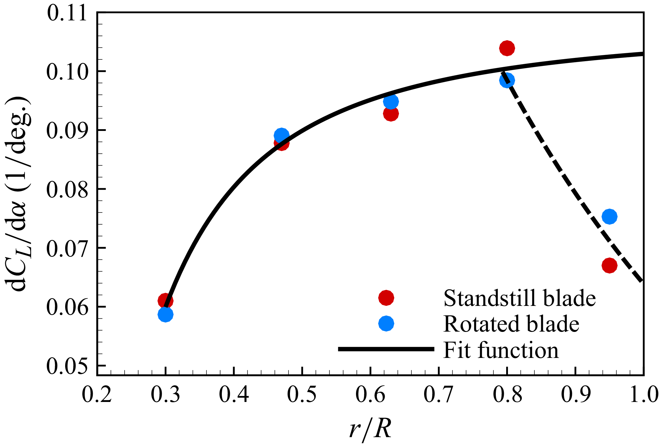
 dCL/dα
 r/R
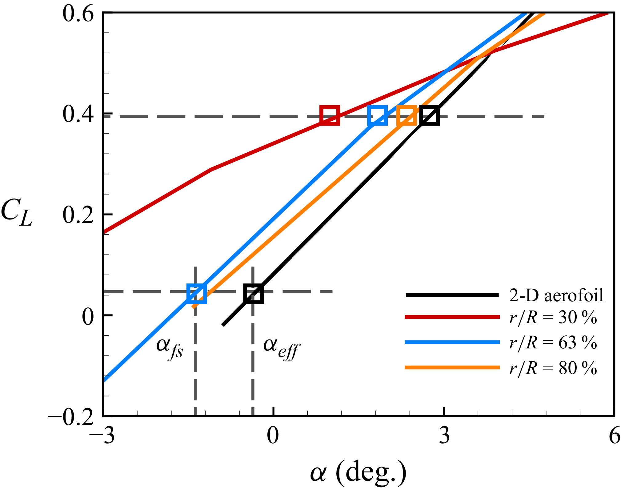
 αeff

 αfs
 ∘
 αfs
 ∘
 αfs
 ∘

 U0
 U0
 U0

 β
 ∘
 β
 ∘

 U0
 U0
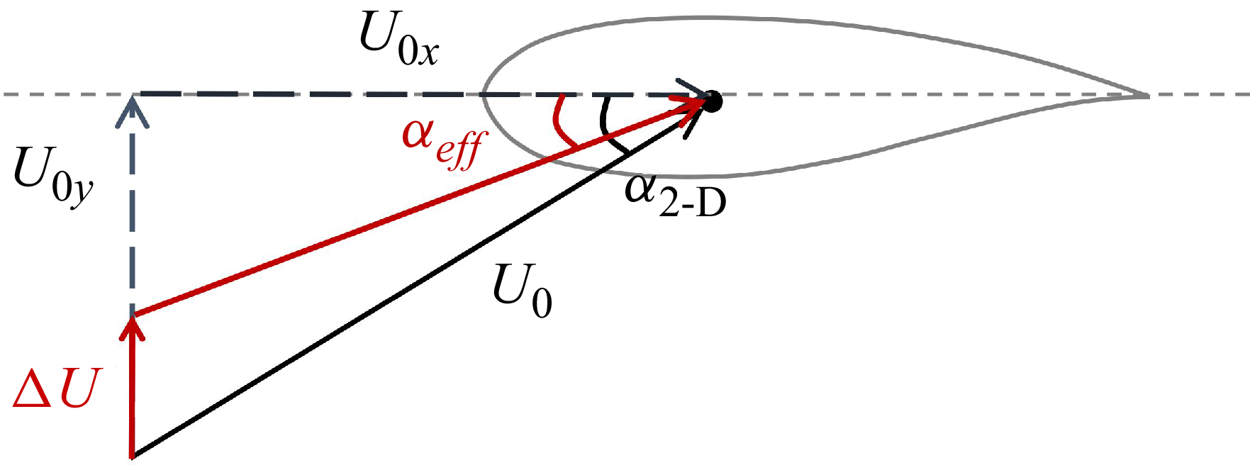
 αeff
 ΔU
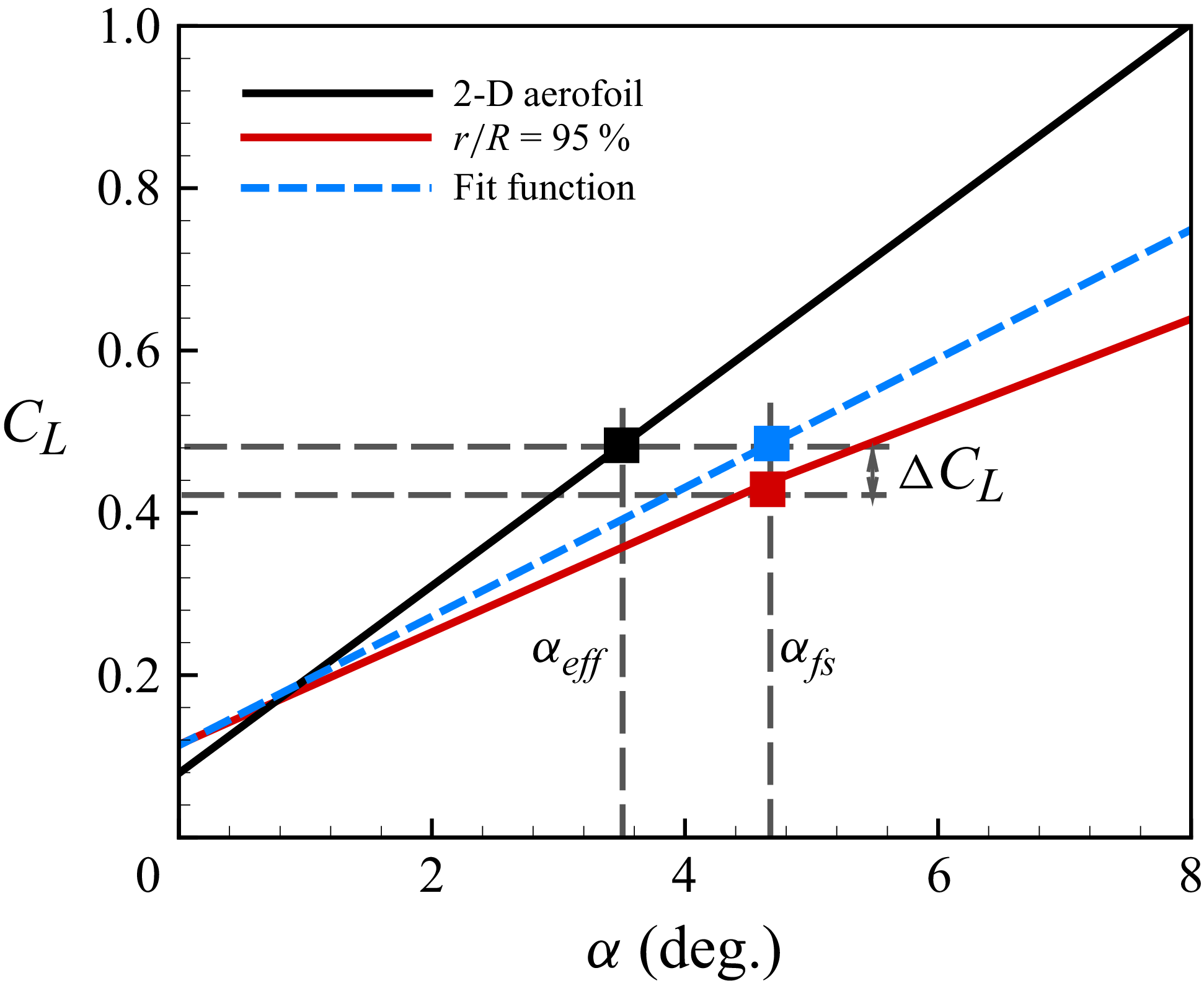
 αeff
 ΔCL

 αfs
 ∘
 αfs
 ∘
 αfs
 ∘

 U0
 U0
 U0

 u/U0
 β
 =86∘
 β
 =81∘

 αeff
 u/U0
 v/U0
 Cp

 dCpt
 β=86∘
 r/R=47%
 80%
 95%
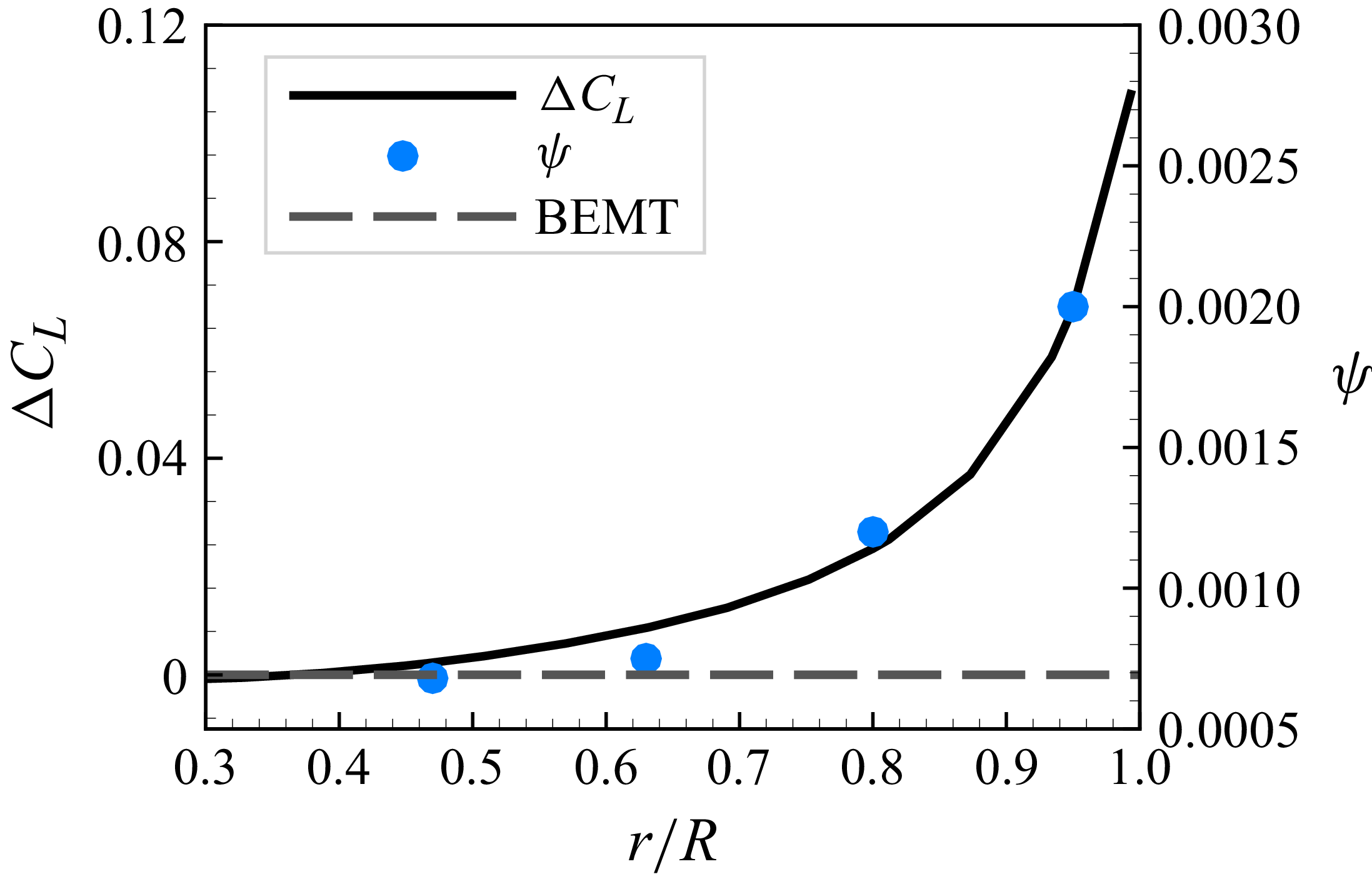
 ψ
 ΔCL
 β=86∘

 Q=3.0
 β
 =86∘
 β
 =80∘

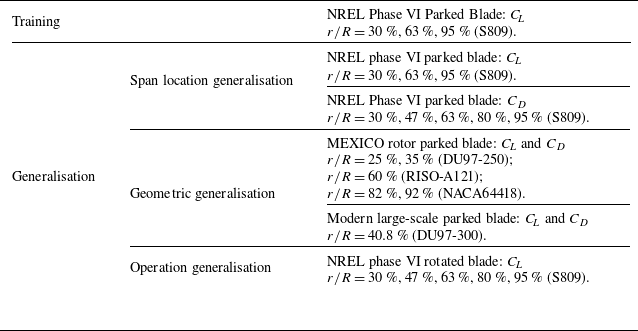

 Fa
 Fr

 Fa
 α2-D
 ∘
 ∘
 Fa
 Fa
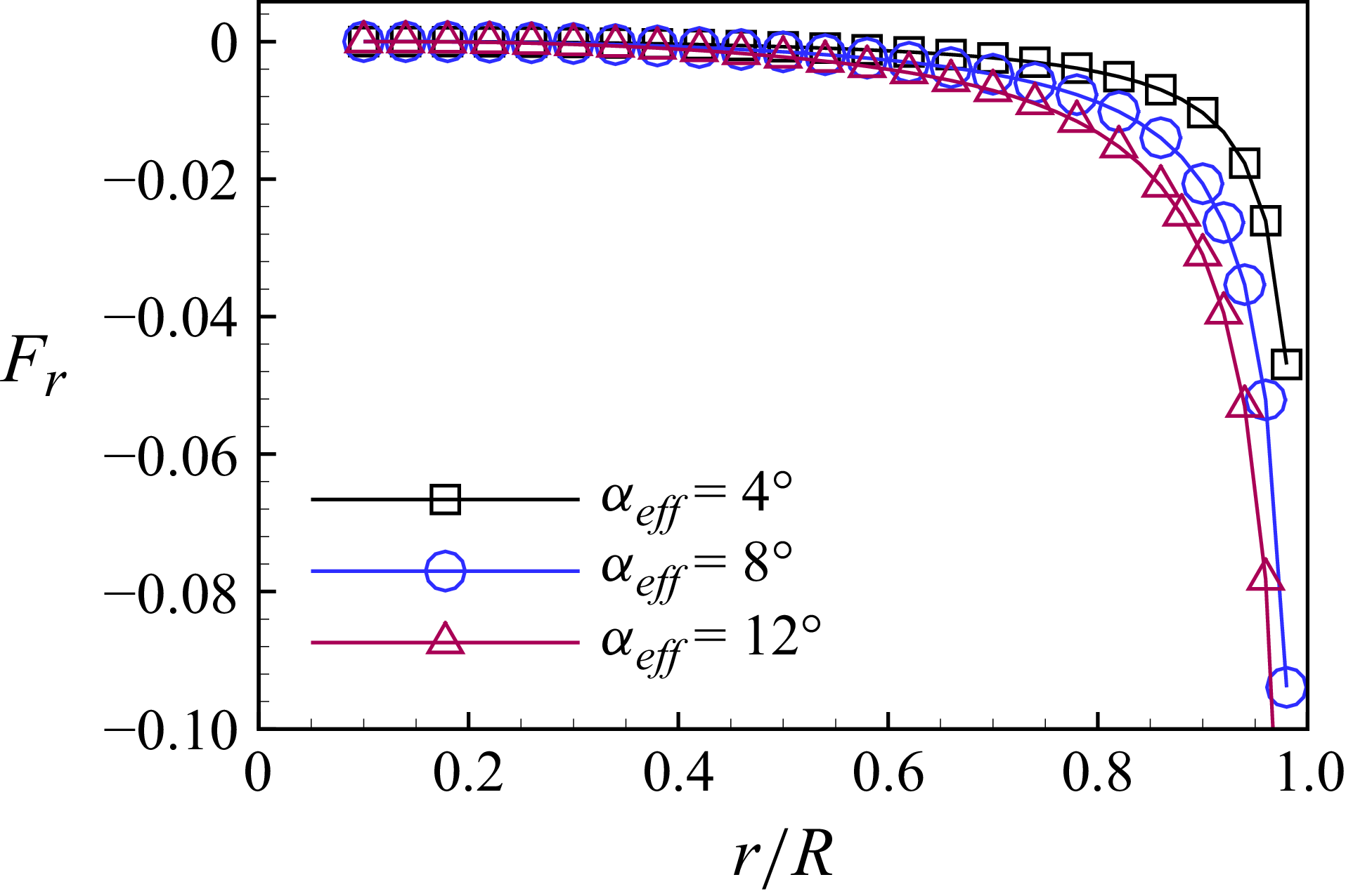
 Fr
 αeff
 ∘
 ∘
 Fr

 r/R
 r/R
 r/R
 r/R
 r/R

 r/R
 r/R
 r/R
 r/R
 r/R
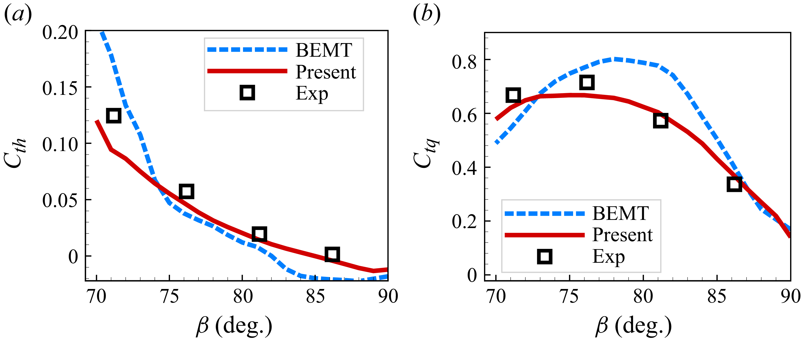
 Cth
 Ctq
 ∘
 ∘
 Cth
 Ctq

 r/R
 r/R
 r/R
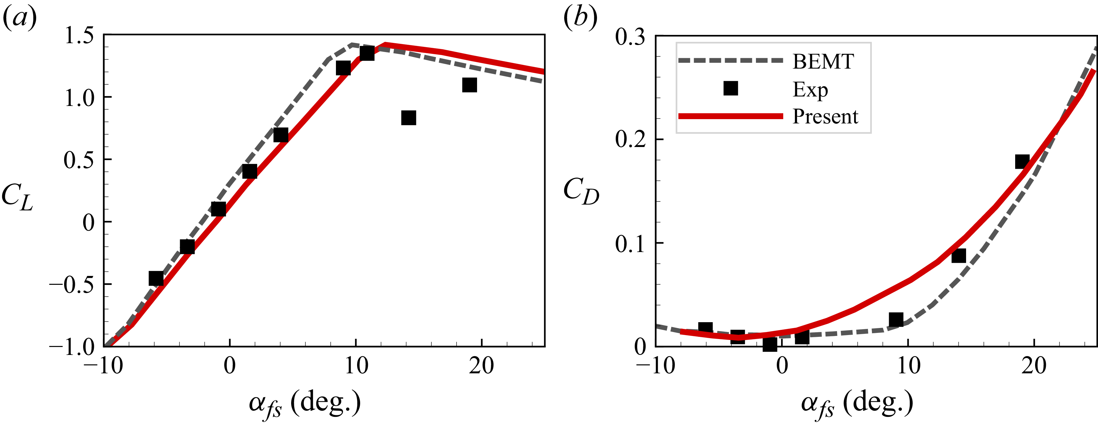

 r/R
 r/R
 r/R
 r/R
 r/R
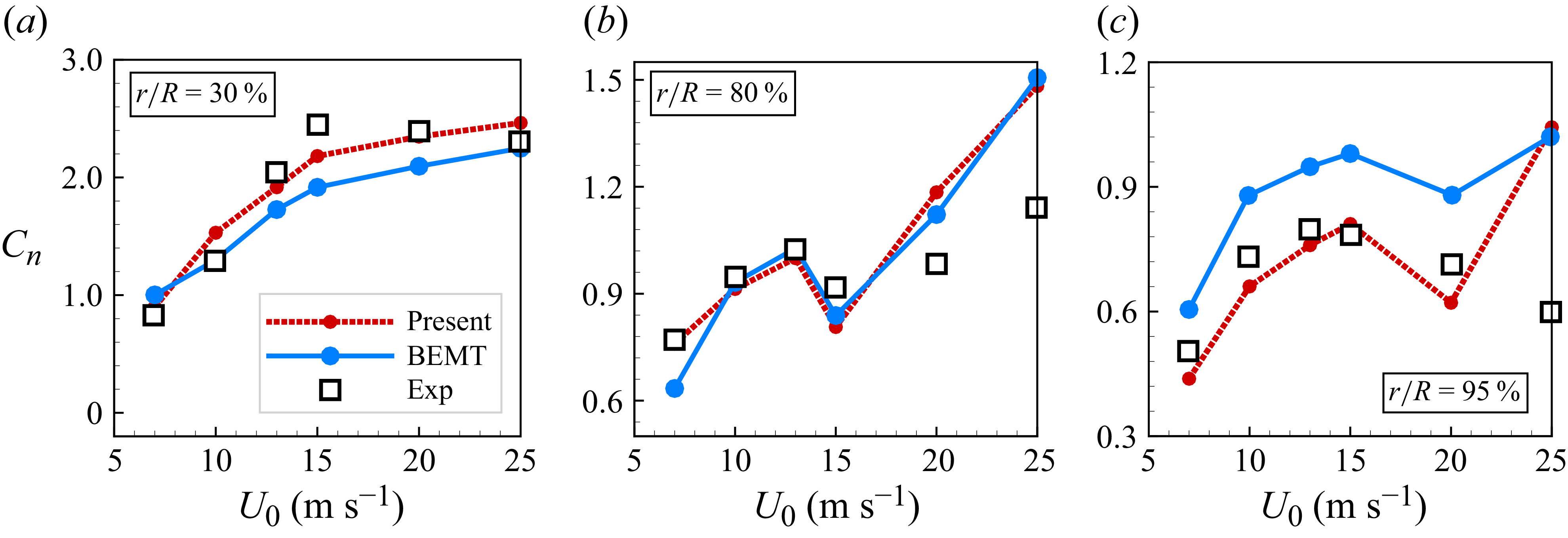
 r/R=30%
 r/R=80%
 r/R=95%
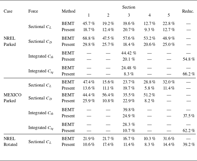

 vd
 β=86∘
 β=76∘
 Q
 Q=3.0
 Fa
 Fr

 β=86∘

 β=76∘
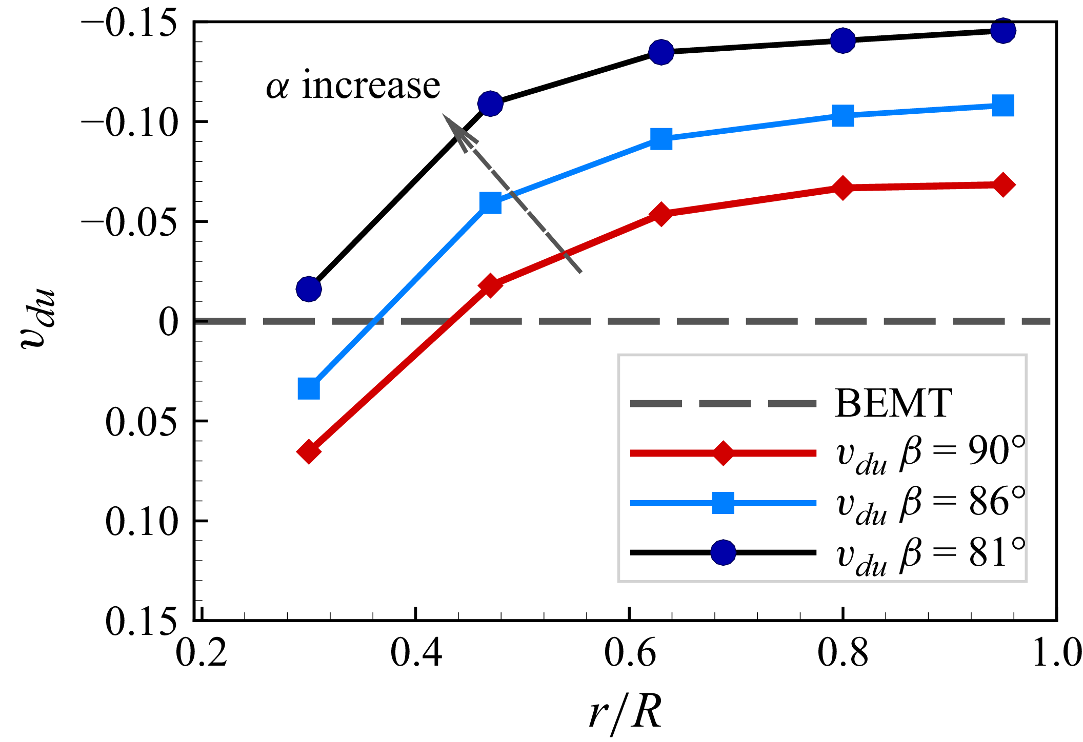
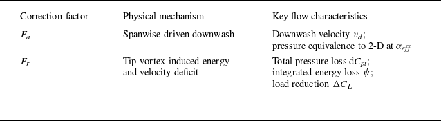

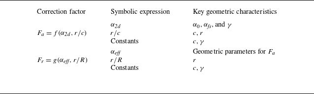


 X
 Y
 x
 y
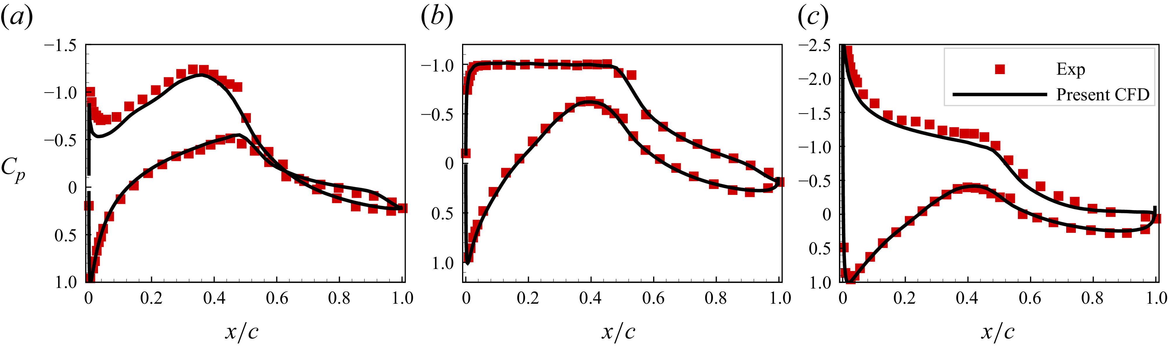
 α=−4.1∘
 α=4.1∘
 α=8.1∘

 75∘
 r/R
 r/R
 r/R
 r/R
 r/R


 U0
 r/R
 r/R
 r/R
 r/R
 r/R
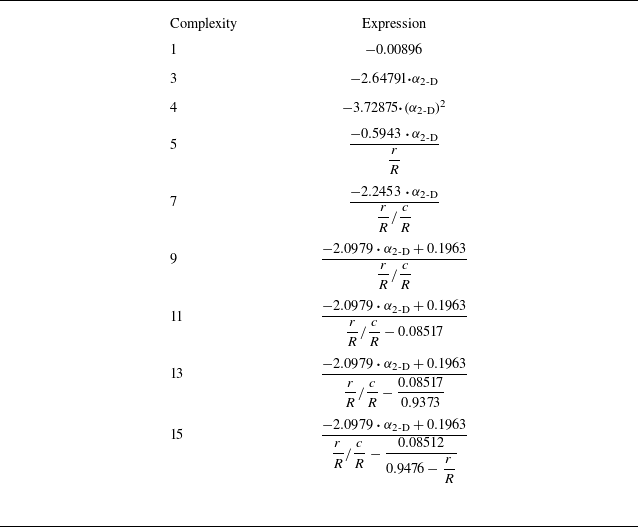
 Fa
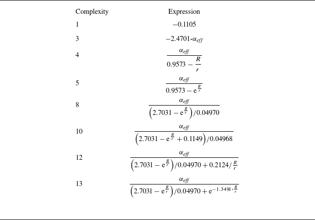
 Fr
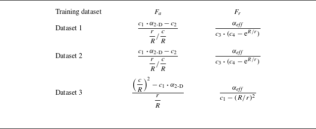
 Fa
 Fr
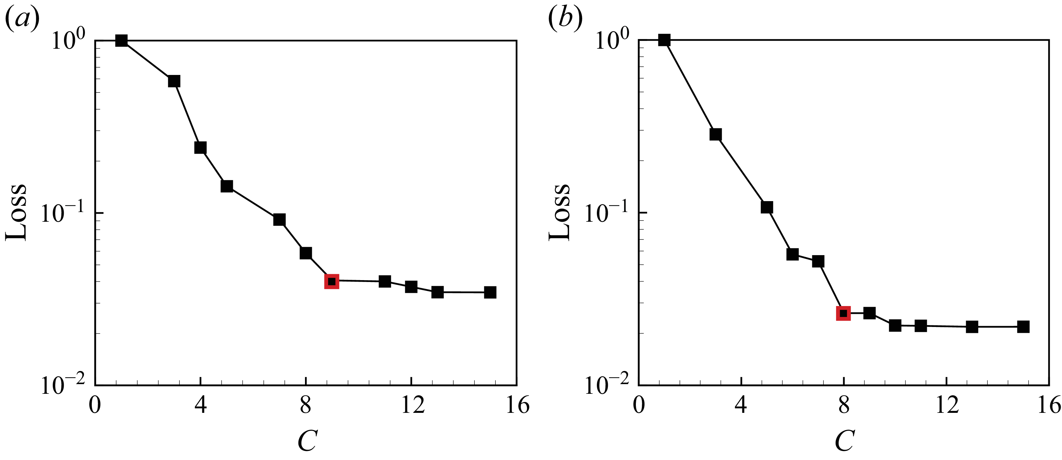
 C
 Fa
 Fr
 Fa
 Fr
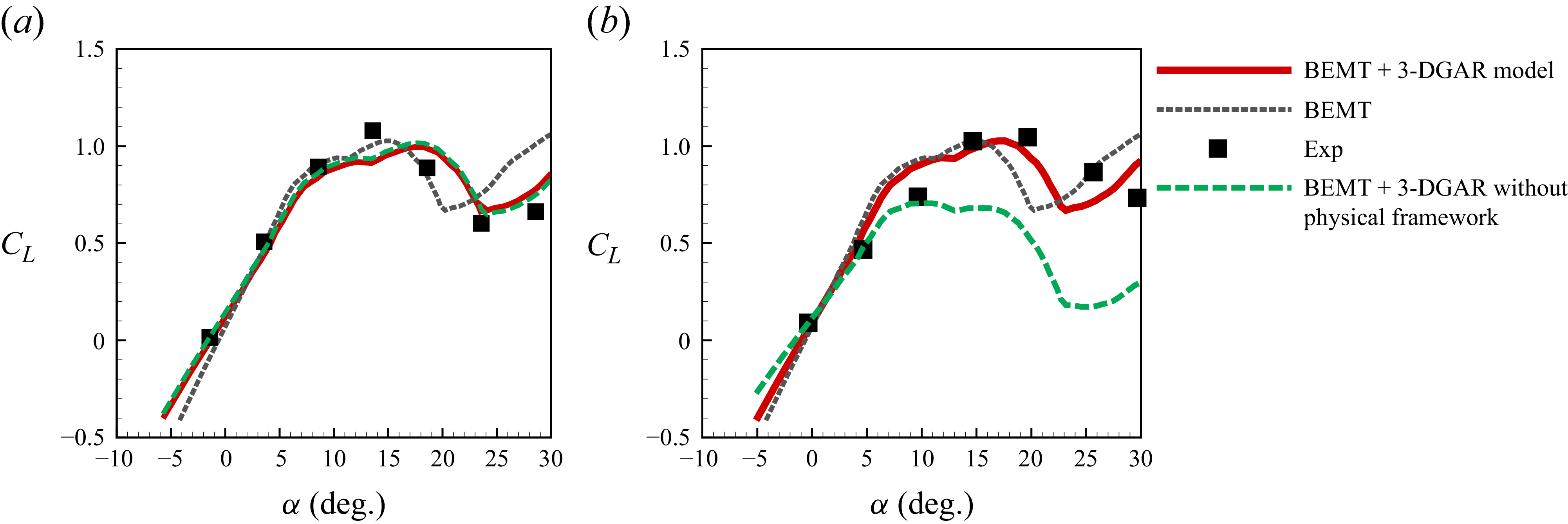
 r/R
 r/R


