1. Introduction
Instabilities in core–annular flows of two miscible fluids (i.e. consist of one fluid in the core and the other fluid in the annular region of a pipe) have been extensively studied due to their relevance in many industrial applications, e.g. transportation of crude oil in pipelines, polymer deposition and extrusion, food processing industries, etc. (Homsy Reference Homsy1987; Selvam et al. Reference Selvam, Merk, Govindarajan and Meiburg2007; Govindarajan & Sahu Reference Govindarajan and Sahu2014). Viscosity stratified flows can also be observed in natural phenomena, e.g. turbidity current (Nasr-Azadani & Meiburg Reference Nasr-Azadani and Meiburg2014). In these flow systems, viscosity stratification is achieved due to the presence of single scalar or multiple scalars diffusing at different rates, such as concentration of a species, temperature etc. Here, the former and the latter systems are termed as single-component (SC) and double-diffusive (DD) flows, respectively. More explicitly, SC systems are the flows having a pure solvent and a solution of the same solvent containing a species at a particular concentration. On the other hand, when the viscosity stratification results from not one, but two species of different diffusivities, the systems are referred to as double-diffusive (DD) systems.
There have been many studies of buoyancy-driven flows in which double diffusion affects density (Turner Reference Turner1974; Taghavi et al. Reference Taghavi, Séon, Martinez and Frigaard2009) but far fewer studies of pressure-driven flows in which double diffusion affects viscosity (see e.g. Mishra et al. Reference Mishra, Trevelyan, Almarcha and De Wit2010; Sahu Reference Sahu2013). The instabilities associated with density-stratified systems are not discussed further, as the focus of the present study is to isolate the effect of viscosity stratification due to the presence of two scalars diffusing at different rates, and to investigate the instabilities in an otherwise stable core–annular pipe flow. This problem has not been investigated yet to the best of the author’s knowledge.
It is well known that flow through a circular pipe is very different from flow through a planar channel even in constant viscosity systems. Classical linear stability analysis has shown that channel flow of a constant viscosity fluid is linearly unstable for Reynolds number,
 $Re>5772.2$
, whereas Hagen–Poiseuille pipe flow is stable for any
 $Re$
(Schmid & Henningson Reference Schmid and Henningson2001).
Let us now discuss what happens in single-component (SC) three-layer flows of two miscible fluids in planar channels. By conducting linear stability analysis in a three-layer channel flow, Ranganathan & Govindarajan (Reference Ranganathan and Govindarajan2001) and Govindarajan (Reference Govindarajan2004) showed that laminar flow becomes unstable when the near wall fluid is more viscous than the fluid in the central region of the channel. In addition to the Tollmien–Schlichting (TS) mode, a new mode of instability was found at low Reynolds number (
 $Re$
) and high diffusivity, when the critical layer (a location where the axial velocity is equal to the phase speed of dominant mode) overlaps with the mixed layer of varying viscosity. On the other hand, a large stabilization occurs in the opposite configuration when the less viscous fluid is placed at the near wall region (Govindarajan Reference Govindarajan2004). In the unstable configuration by conducting a linear stability analysis, Sahu et al. (Reference Sahu, Ding, Valluri and Matar2009) found that the flow is absolutely unstable under certain parameter ranges, which in turn takes the flow towards a transitional state via a nonlinear mechanism.
In the case of core–annular miscible SC flows in cylindrical pipes, several authors (Lajeunesse et al. Reference Lajeunesse, Martin, Rakotomalala and Salin1997, Reference Lajeunesse, Martin, Rakotomalala, Salin and Yortsos1999; Scoffoni, Lajeunesse & Homsy Reference Scoffoni, Lajeunesse and Homsy2001; Selvam et al. Reference Selvam, Talon, Lesshafft and Meiburg2009) have examined the development of axisymmetric and corkscrew patterns. Similar instability patterns were also observed in the experiment of d’Olce et al. (Reference d’Olce, Martin, Rakotomalala, Salin and Talon2008) in the case of neutrally buoyant, miscible core–annular flows in horizontal pipes at high Schmidt and Reynolds numbers. Selvam et al. (Reference Selvam, Merk, Govindarajan and Meiburg2007) conducted linear stability analysis for a core–annular flow in a pipe, and showed that beyond a critical viscosity ratio, the flow is unstable even when the less viscous fluid is at the wall, in contrast to immiscible lubricated pipelining (Joseph et al. Reference Joseph, Bai, Chen and Renardy1997) and to miscible planar channel flows (Govindarajan Reference Govindarajan2004; Malik & Hooper Reference Malik and Hooper2005; Sahu et al. Reference Sahu, Ding, Valluri and Matar2009) which are stable in this configuration. Selvam et al. (Reference Selvam, Merk, Govindarajan and Meiburg2007) also showed that the axisymmetric (corkscrew) mode is dominant if the pipe core is occupied with the more (less) viscous fluid. This is in contrast with the single fluid pipe flow (the Hagen–Poiseuille flow), for which the corkscrew mode is always the least stable one.
The investigations discussed so far are for SC systems. One objective of the present study is to identify the differences between the DD systems and their SC counterparts. The instability due to the DD effect in miscible flows of two fluids having different viscosities has received comparatively less attention than that received by SC systems. By conducting linear stability analysis, Sahu & Govindarajan (Reference Sahu and Govindarajan2011) investigated the instability associated with DD phenomenon in a three-layer channel configuration, wherein viscosity decreases towards the wall. As discussed above, this is a stable configuration in the context of SC flows as the less viscous fluid present in the near wall region essentially acts as a lubricating fluid (Ranganathan & Govindarajan Reference Ranganathan and Govindarajan2001). Their results show the existence of an unstable DD mode at low
 $Re$
(about 100) in this classically stable configuration (Sahu & Govindarajan Reference Sahu and Govindarajan2011). The DD system is observed to exhibit instability characteristics which are fundamentally different from those shown by SC systems. Their investigation clearly demonstrates the significance of viscosity stratification in a double-diffusive three-layer channel flow. In a similar system with DD effect, Sahu & Govindarajan (Reference Sahu and Govindarajan2012) demonstrated the appearance of a rapidly growing absolute instability, which is only convectively unstable without the presence of DD phenomenon. The instabilities due to the influence of DD effect were also observed in other flow systems, e.g. displacement of a highly viscous fluid by a less viscous one in porous media (Swernath & Pushpavanam Reference Swernath and Pushpavanam2007; Mishra et al.
Reference Mishra, Trevelyan, Almarcha and De Wit2010), Hele-Shaw cell (Pritchard Reference Pritchard2009), and in pressure-driven flow in a channel (Mishra, De Wit & Sahu Reference Mishra, De Wit and Sahu2012). A review of instabilities associated with DD effect in various flow configurations can be found in Govindarajan & Sahu (Reference Govindarajan and Sahu2014).
Recently, Bhagat, Tripathi & Sahu (Reference Bhagat, Tripathi and Sahu2016) numerically investigated displacement flow of a less viscous fluid initially occupying an entire pipe by a highly viscous fluid injected at the inlet, in the presence of DD effect. They found instability due to the DD phenomenon in a classically stable configuration in the context of SC flows (Saffman & Taylor Reference Saffman and Taylor1958). The present work differs from that of Bhagat et al. (Reference Bhagat, Tripathi and Sahu2016) in two ways: (i) the geometry considered in the present study is a core–annular configuration, whereas Bhagat et al. (Reference Bhagat, Tripathi and Sahu2016) studied a displacement flow of one fluid by another one, and (ii) they performed numerical simulations of a displacement flow in an extended pipe, on the other hand, the objective of the present work is to study instabilities associated with a core–annular flow in linear and nonlinear regimes via linear stability analysis and direct numerical simulations.
As the above brief review shows, all the previous work carried out on the DD effect has so far been for planar channels (except the recent study of Bhagat et al. (Reference Bhagat, Tripathi and Sahu2016)) although cylindrical geometries are frequently encountered in industrial applications. Hence, the main goal of the present work is to establish the differences between viscosity-stratified core–annular flows with their planar counterparts in the presence of the DD effect. In the present work, a core–annular pipe flow in the presence of the DD effect is investigated via a temporal linear analysis and axisymmetric direct numerical simulations. It is shown that the flow which is stable in the context of SC systems, now becomes unstable in the presence of the DD effect. Increasing the diffusivity ratio of the faster and the slower-diffusing scalars enhances the instability. It is shown that the faster-growing axisymmetric mode is more unstable than the corresponding corkscrew mode for the parameter values considered in this work, whereas the equivalent SC flows are stable to all the modes. The diffusion and the radial location of the mixed layer are found to have non-monotonic effects on the instability characteristics. An energy budget analysis and inviscid stability theory are conducted in order to understand the underlying mechanism of the instability in the DD pipe flow. The study of linear instability due to the DD phenomenon is extended to the nonlinear regime via direct numerical simulations.
The rest of this paper is organised as follows. The problem is formulated and the governing linear stability equations are derived in § 2. The results obtained from the linear stability analysis are discussed in § 3, wherein a parametric study is conducted to investigate the effects of the diffusivity ratio, location and thickness of the mixed layer. The results obtained from the direct numerical simulations are presented in § 4. Concluding remarks are provided in § 5.
2. Formulation
The linear stability characteristics and direct numerical simulations of a pressure-driven core–annular flow of two miscible fluids consisting of two scalars diffusing at different rates in a rigid and impermeable pipe of radius
 $R$
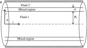
is considered. A schematic diagram of the system is shown in figure 1. The fluids are Newtonian and incompressible of equal densities and different viscosities. A cylindrical coordinate system
 $(r,{\it\theta},z)$
, where
 $r$
,
 ${\it\theta}$
and
 $z$
denote the radial, the azimuthal and the axial coordinates, respectively, is used. The core fluid of viscosity
 ${\it\mu}_{1}$
(fluid ‘1’), which is located in the region
 $0\leqslant r\leqslant R_{1}$
, contains the slower- and the faster-diffusing scalars,
 $S$
and
 $F$
, respectively, in quantities
 $S_{1}$
and
 $F_{1}$
. Another fluid of viscosity
 ${\it\mu}_{2}$
(fluid ‘2’), containing the slower- and the faster-diffusing scalars in quantity
 $S_{2}$
and
 $F_{2}$
, occupies the annular region of the pipe
 $(R_{1}+q<r<R)$
. The fluids are separated by a mixed layer of uniform thickness
 $q$
(Selvam et al.
Reference Selvam, Merk, Govindarajan and Meiburg2007; Sahu & Govindarajan Reference Sahu and Govindarajan2011). The parallel flow approximation is employed in prescribing the thickness
 $q$
to be uniform. The diffusion of the two fluids is proportional to the inverse of the Péclet number
 $(Pe=ScRe)$
;
 $Re$
and
 $Sc$
are Reynolds and Schmidt numbers defined below. As the minimum Reynolds numbers considered in this study is
 $O(10^{2})$
, the parallel flow approximation is justified unless
 $Sc\ll 1$
.
Schematic of the flow configuration considered. Fluids ‘1’ and ‘2’ occupy the core
 $(0\leqslant r\leqslant R_{1})$
and annular
 $(R_{1}+q<r<R)$
regions of the pipe, respectively. The fluids are separated by a mixed layer of uniform thickness
 $q$
.

The dynamic viscosity,
 ${\it\mu}$
is assumed to be an exponential function of the concentration of the scalars:
 $$\begin{eqnarray}{\it\mu}={\it\mu}_{1}\exp \left[R_{s}\left(\frac{S-S_{1}}{S_{2}-S_{1}}\right)+R_{f}\left(\frac{F-F_{1}}{F_{2}-F_{1}}\right)\right],\end{eqnarray}$$
where
 $R_{s}\,(\equiv (S_{2}-S_{1})\text{d}(\ln {\it\mu})/\text{d}S)$
and
 $R_{f}\,(\equiv (F_{2}-F_{1})\text{d}(\ln {\it\mu})/\text{d}F)$
are the log-mobility ratios of the slower- and faster-diffusing scalars, respectively.
The flow dynamics are governed by the incompressible form of continuity and Navier–Stokes equations along with the convection-diffusion equations for both the scalars:
 $$\begin{eqnarray}\displaystyle & \displaystyle \boldsymbol{{\rm\nabla}}\boldsymbol{\cdot }\boldsymbol{u}=0, & \displaystyle\end{eqnarray}$$
 $$\begin{eqnarray}\displaystyle & \displaystyle {\it\rho}\left[\frac{\partial \boldsymbol{u}}{\partial t}+\boldsymbol{u}\boldsymbol{\cdot }\boldsymbol{{\rm\nabla}}\boldsymbol{u}\right]=-\boldsymbol{{\rm\nabla}}p+\boldsymbol{{\rm\nabla}}\boldsymbol{\cdot }[{\it\mu}(\boldsymbol{{\rm\nabla}}\boldsymbol{u}+\boldsymbol{{\rm\nabla}}\boldsymbol{u}^{\text{T}})], & \displaystyle\end{eqnarray}$$
 $$\begin{eqnarray}\displaystyle & \displaystyle \frac{\partial S}{\partial t}+\boldsymbol{u}\boldsymbol{\cdot }\boldsymbol{{\rm\nabla}}S=\mathscr{D}_{s}{\rm\nabla}^{2}S, & \displaystyle\end{eqnarray}$$
 $$\begin{eqnarray}\displaystyle & \displaystyle \frac{\partial F}{\partial t}+\boldsymbol{u}\boldsymbol{\cdot }\boldsymbol{{\rm\nabla}}F=\mathscr{D}_{f}{\rm\nabla}^{2}F, & \displaystyle\end{eqnarray}$$
 $\boldsymbol{u}\equiv ({u_{r}}_{T},{u_{{\it\theta}}}_{T},{u_{z}}_{T})$
is the velocity vector and
 ${u_{r}}_{T}$
,
 ${u_{{\it\theta}}}_{T}$
and
 ${u_{z}}_{T}$
are the velocity components in the radial, the azimuthal and the axial directions, respectively,
 $t$
is time and
 $p$
denotes pressure.
 $\mathscr{D}_{s}$
and
 $\mathscr{D}_{f}$
are the diffusion coefficients of the slower- and the faster-diffusing scalars, respectively. Thus by definition
 $\mathscr{D}_{f}>\mathscr{D}_{s}$
, and
 ${\it\delta}\,(\equiv \mathscr{D}_{f}/\mathscr{D}_{s})$
is greater than or equal to one;
 ${\it\delta}=1$
represents a system having scalars of equal diffusion coefficients.
Equations (2.1)–(2.2) are non-dimensionalised using the radius of the pipe
 $(R)$
as the length scale and
 $V\,(\equiv Q/{\rm\pi}R^{2})$
as the velocity scale, where
 $Q$
denotes the volumetric flow rate. The following scaling is employed to render the governing equations dimensionless:
 $$\begin{eqnarray}\displaystyle \left.\begin{array}{@{}c@{}}\displaystyle (r,z,q,R_{1})=R(\,\widetilde{r},\widetilde{z},\widetilde{q},\widetilde{R}_{1}),\quad t=\frac{R}{V}\widetilde{t},\\ \displaystyle ({u_{r}}_{T},{u_{{\it\theta}}}_{T},{u_{z}}_{T})=V(\widetilde{u_{r}}_{T},\widetilde{u_{{\it\theta}}}_{T},\widetilde{u_{z}}_{T}),\quad p={\it\rho}V^{2}\widetilde{p},\\ \displaystyle {\it\mu}=\widetilde{{\it\mu}}{\it\mu}_{1},\quad \widetilde{s}=\frac{S-S_{1}}{S_{2}-S_{1}},\quad \widetilde{f}=\frac{F-F_{1}}{F_{2}-F_{1}},\end{array}\right\} & & \displaystyle\end{eqnarray}$$
where tildes designate dimensionless quantities and
 ${\it\rho}$
is the constant density. After dropping the tildes decoration, the dimensionless governing equations are given by
 $$\begin{eqnarray}\displaystyle & \displaystyle \boldsymbol{{\rm\nabla}}\boldsymbol{\cdot }\boldsymbol{u}=0, & \displaystyle\end{eqnarray}$$
 $$\begin{eqnarray}\displaystyle & \displaystyle \left[\frac{\partial \boldsymbol{u}}{\partial t}+\boldsymbol{u}\boldsymbol{\cdot }\boldsymbol{{\rm\nabla}}\boldsymbol{u}\right]=-\boldsymbol{{\rm\nabla}}p+\frac{1}{Re}\boldsymbol{{\rm\nabla}}\boldsymbol{\cdot }[{\it\mu}(\boldsymbol{{\rm\nabla}}\boldsymbol{u}+\boldsymbol{{\rm\nabla}}\boldsymbol{u}^{\text{T}})], & \displaystyle\end{eqnarray}$$
 $$\begin{eqnarray}\displaystyle & \displaystyle \frac{\partial s}{\partial t}+\boldsymbol{u}\boldsymbol{\cdot }\boldsymbol{{\rm\nabla}}s=\frac{1}{Re\,Sc}{\rm\nabla}^{2}s, & \displaystyle\end{eqnarray}$$
 $$\begin{eqnarray}\displaystyle & \displaystyle \frac{\partial f}{\partial t}+\boldsymbol{u}\boldsymbol{\cdot }\boldsymbol{{\rm\nabla}}f=\frac{{\it\delta}}{Re\,Sc}{\rm\nabla}^{2}f, & \displaystyle\end{eqnarray}$$
 $Re\,(\equiv {\it\rho}VR/{\it\mu}_{1})$
,
 $Sc\,(\equiv {\it\mu}_{1}/{\it\rho}\mathscr{D}_{s})$
are the Reynolds number and Schmidt numbers, respectively, which are defined based on the slower-diffusing scalar. Thus, the effective Schmidt number of the faster-diffusing fluid is
 $Sc/{\it\delta}$
.
The dimensionless viscosity,
 ${\it\mu}$
is given by
 $$\begin{eqnarray}{\it\mu}=\exp (R_{s}s+R_{f}f).\end{eqnarray}$$
Here,
 $R_{s}+R_{f}>0\,({<}0)$
represents a configuration when the annular fluid is more (less) viscous than the core fluid. The focus of the present study is to investigate the instability of systems which are stable in the context of single component flows.
2.1. Linear stability analysis
2.1.1. Basic state
The basic state whose linear stability characteristics will be analysed corresponds to a steady, parallel, fully-developed flow, i.e.
 $U_{r}=U_{{\it\theta}}=0;U_{z}=U_{z}(r)$
and
 $P$
is linear in
 $z$
. This is obtained by solving the steady, fully-developed version of (2.8), i.e.
 $$\begin{eqnarray}\frac{1}{r}\frac{\partial }{\partial r}\left[r{\it\mu}_{0}\frac{\partial U_{z}}{\partial r}\right]=\frac{\text{d}P}{\text{d}z}Re,\end{eqnarray}$$
subject to the no-slip and the symmetric boundary conditions at the pipe wall and the centreline of the channel, respectively. The dimensionless pressure gradient
 $\text{d}P/\text{d}z$
is fixed by using
 $\int _{0}^{1}U_{z}r\,\text{d}r=1$
. Here
 ${\it\mu}_{0}=\text{e}^{(R_{s}s_{0}+R_{f}f_{0})}$
. The basic state quantities are designated by upper-case letters for the flow variables, and by the subscript
 $0$
for viscosity,
 $s$
and
 $f$
. In order to make the concentration of the scalars continuous up to the second derivative at
 $r=R_{1}$
and
 $r=R_{1}+q$
, the scalars
 $s_{0}$
and
 $f_{0}$
are chosen to be fifth order polynomials in the mixed layer (Sahu & Govindarajan Reference Sahu and Govindarajan2011):
 $$\begin{eqnarray}\displaystyle s_{0}=\left\{\begin{array}{@{}ll@{}}\displaystyle f_{0}=0,\quad & \displaystyle 0\leqslant r\leqslant R_{1},\\ \displaystyle f_{0}=\mathop{\sum }_{i=1}^{6}a_{i}r^{i-1},\quad & \displaystyle R_{1}\leqslant r\leqslant R_{1}+q,\\ \displaystyle f_{0}=1,\quad & \displaystyle R_{1}+q\leqslant r\leqslant 1,\end{array}\right. & & \displaystyle\end{eqnarray}$$
where
 $a_{i}~(i=1,6)$
are given by
 $$\begin{eqnarray}\displaystyle \left.\begin{array}{@{}c@{}}\displaystyle a_{1}=-\frac{{R_{1}}^{3}}{q^{5}}(6R_{1}^{2}+15R_{1}q+10q^{2}),\quad a_{2}=\frac{30{R_{1}}^{2}}{q^{5}}(R_{1}+q)^{2},\\ \displaystyle a_{3}=-\frac{30R_{1}}{q^{5}}(R_{1}+q)(2R_{1}+q),\quad a_{4}=\frac{10}{q^{5}}(6R_{1}^{2}+6R_{1}q+q^{2}),\\ \displaystyle a_{5}=-\frac{15}{q^{5}}(2R_{1}+q)\quad \text{and}\quad a_{6}=\frac{6}{q^{5}}.\end{array}\right\} & & \displaystyle\end{eqnarray}$$
It has been confirmed that the other sufficiently smooth profiles, such as the one used by Selvam et al. (Reference Selvam, Merk, Govindarajan and Meiburg2007):
 $$\begin{eqnarray}s_{0}=f_{0}=0.5+0.5\,\text{erf}\left[\frac{r-R_{1}-0.5q}{0.25q}\right],\end{eqnarray}$$
also gives results practically indistinguishable from those presented here. The validity of the basic state considered in this study is discussed in appendix C.
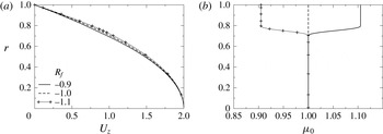
Typical basic state profiles of axial velocity
 $(U_{z})$
and viscosity
 $({\it\mu}_{0})$
are shown for different values of
 $R_{f}$
in figures 2(a) and 2(b), respectively. The rest of the parameters are chosen as
 $R_{1}=0.7$
,
 $q=0.1$
and
 $R_{s}=1$
. In figure 2(a), it can be seen that the basic state axial velocity at the mixed region increases with decreasing the value of
 $R_{f}$
. It is also seen that for
 $R_{f}=-0.9$
and
 $-1.1$
, the annular fluid is respectively more and less viscous than the fluid occupying the core of the pipe;
 $R_{f}=-1$
means that both fluids are of equal viscosities (single-component (SC) system), as
 $R_{s}=1$
. In three-layer SC channel flows, it is well known that when the near wall fluid is less viscous, the velocity profile goes away from the inflectional profile (i.e. profile with
 $U_{z}^{\prime \prime }=0$
) and thus has a stabilising influence (Govindarajan Reference Govindarajan2004). However, for pipe flows, Selvam et al. (Reference Selvam, Merk, Govindarajan and Meiburg2007) showed that an axisymmetric mode becomes unstable above a critical viscosity ratio even when the annular fluid is less viscous. These aspects will be discussed again in the following section.
Basic state profiles of (a) axial velocity (b) viscosity, for different values of
 $R_{f}$
. The rest of the parameter values are
 $R_{1}=0.7$
,
 $q=0.1$
and
 $R_{s}=1$
.

2.1.2. Linear stability equations
We investigate the temporal stability of the basic flow given by (2.12)–(2.13) to infinitesimal perturbations using a normal mode analysis by expressing each flow variable as a sum of the basic state and a time-dependent perturbation (designated by a hat):
 $$\begin{eqnarray}\displaystyle ({u_{r}}_{T},{u_{{\it\theta}}}_{T},{u_{z}}_{T},p,s,f)(r,{\it\theta},z,t) & = & \displaystyle (0,0,U_{z}(r),P,s_{0}(r),f_{0}(r))\nonumber\\ \displaystyle & & \displaystyle +\,(\text{i}\hat{u} _{r},\hat{u} _{{\it\theta}},\hat{u} _{z},\hat{p},{\hat{s}},\hat{f})(r)\text{e}^{\text{i}({\it\alpha}z+{\it\beta}{\it\theta}-{\it\omega}t)},\end{eqnarray}$$
where
 $\text{i}\equiv \sqrt{-1}$
,
 ${\it\alpha}$
,
 ${\it\beta}$
and
 ${\it\omega}\,(\equiv {\it\alpha}c)$
are the wavenumbers in the axial and the azimuthal directions (real) and the frequency (complex) of the perturbation, respectively, wherein
 $c\,(\equiv c_{r}+\text{i}c_{i})$
is the phase speed of the perturbation. The subscripts
 $r$
and
 $i$
represent the real and imaginary parts, respectively. Here, a given mode is unstable if
 ${\it\omega}_{i}>0$
, stable if
 ${\it\omega}_{i}<0$
and neutrally stable if
 ${\it\omega}_{i}=0$
. The perturbation viscosity is given by:
 $\hat{{\it\mu}}=(\partial {\it\mu}_{0}/\partial s_{0}){\hat{s}}+(\partial {\it\mu}_{0}/\partial f_{0})\hat{f}.$
Following the standard procedure (Schmid & Henningson Reference Schmid and Henningson2001): (i) substitution of (2.16) into (2.7)–(2.10), (ii) subtraction of the basic state equations, and (iii) linearization and elimination of the pressure perturbation, we obtained the following linear stability equations (suppressing the hat notations):
 $$\begin{eqnarray}\displaystyle u_{r}^{\prime }+\frac{u_{r}}{r}+\frac{{\it\beta}u_{{\it\theta}}}{r}+{\it\alpha}u_{z}=0, & & \displaystyle\end{eqnarray}$$
 $$\begin{eqnarray}\displaystyle -{\it\omega}u_{r}+{\it\alpha}u_{r}U_{z} & = & \displaystyle \displaystyle p^{\prime }-\frac{\text{i}}{Re}\left[{\it\mu}_{0}\left\{u_{r}^{\prime \prime }+\frac{u_{r}^{\prime }}{r}-\left(\frac{{\it\beta}^{2}+1}{r^{2}}+{\it\alpha}^{2}\right)u_{r}-\frac{2{\it\beta}}{r^{2}}u_{{\it\theta}}\right\}\right.\nonumber\\ \displaystyle & & \displaystyle \displaystyle +\left.2{\it\mu}_{0}^{\prime }u_{r}^{\prime }+{\it\alpha}U_{z}^{\prime }{\it\mu}\right],\end{eqnarray}$$
 $$\begin{eqnarray}\displaystyle -{\it\omega}u_{{\it\theta}}+{\it\alpha}u_{{\it\theta}}U_{z} & = & \displaystyle \displaystyle -\frac{{\it\beta}p}{r}-\frac{\text{i}{\it\mu}_{0}}{Re}\left\{u_{{\it\theta}}^{\prime \prime }+\frac{u_{{\it\theta}}^{\prime }}{r}-\left(\frac{{\it\beta}^{2}+1}{r^{2}}+{\it\alpha}^{2}\right)u_{{\it\theta}}-\frac{2{\it\beta}}{r^{2}}u_{r}\right\}\nonumber\\ \displaystyle & & \displaystyle \displaystyle -\,\frac{\text{i}{\it\mu}_{0}^{\prime }}{Re}\left[u_{{\it\theta}}^{\prime }-\frac{u_{{\it\theta}}}{r}-\frac{{\it\beta}u_{r}}{r}\right],\end{eqnarray}$$
 $$\begin{eqnarray}\displaystyle -{\it\omega}u_{z}+U_{z}^{\prime }u_{r}+{\it\alpha}U_{z}u_{z} & = & \displaystyle \displaystyle -{\it\alpha}p-\frac{\text{i}{\it\mu}_{0}}{Re}\left\{u_{z}^{\prime \prime }+\frac{u_{z}^{\prime }}{r}-\left(\frac{{\it\beta}^{2}}{r^{2}}+{\it\alpha}^{2}\right)u_{z}\right\}\nonumber\\ \displaystyle & & \displaystyle \displaystyle -\,\frac{\text{i}{\it\mu}_{0}^{\prime }}{Re}[v_{z}^{\prime }-{\it\alpha}v_{r}]-\frac{\text{i}U_{z}^{\prime }}{Re}{\it\mu}^{\prime }-\frac{\text{i}{\it\mu}}{Re}\left[U_{z}^{\prime \prime }+\frac{U_{z}^{\prime }}{r}\right],\end{eqnarray}$$
 $$\begin{eqnarray}\displaystyle & \displaystyle -{\it\omega}s+s_{0}^{\prime }u_{r}+{\it\alpha}U_{z}s=-\frac{\text{i}}{Re\,Sc}\left\{s^{\prime \prime }+\frac{s^{\prime }}{r}-\left(\frac{{\it\beta}^{2}}{r^{2}}+{\it\alpha}^{2}\right)s\right\}, & \displaystyle\end{eqnarray}$$
 $$\begin{eqnarray}\displaystyle & \displaystyle -{\it\omega}f+f_{0}^{\prime }u_{r}+{\it\alpha}U_{z}f=-\frac{\text{i}{\it\delta}}{Re\,Sc}\left\{f^{\prime \prime }+\frac{f^{\prime }}{r}-\left(\frac{{\it\beta}^{2}}{r^{2}}+{\it\alpha}^{2}\right)f\right\}, & \displaystyle\end{eqnarray}$$
 $r$
. We confirm that for the no viscosity-stratification case, i.e. by setting
 ${\it\mu}_{0}=1$
, these equations reduce to the stability equations for the Hagen–Poiseuille flow (Schmid & Henningson Reference Schmid and Henningson2001). Solutions of these equations are obtained subject to the following boundary conditions (Sahu & Govindarajan Reference Sahu and Govindarajan2005; Selvam et al.
Reference Selvam, Merk, Govindarajan and Meiburg2007):
At the centreline of the pipe
 $(r=0)$
, the boundary conditions are
 $$\begin{eqnarray}\displaystyle v_{r}=0,\quad v_{{\it\theta}}=0,\quad v_{z}^{\prime }=0,\quad p^{\prime }=0,\quad s^{\prime }=0\quad \text{and}\quad f^{\prime }=0\quad \text{for}\;{\it\beta}=0,\qquad & & \displaystyle\end{eqnarray}$$
 $$\begin{eqnarray}\displaystyle v_{r}+v_{{\it\theta}}=0,\quad 2v_{r}^{\prime }+v_{{\it\theta}}^{\prime }=0,\quad v_{z}=0,\quad p=0,\quad s=0\quad \text{and}\quad f=0\quad \text{for}\;{\it\beta}=1, & & \displaystyle \nonumber\\ \displaystyle & & \displaystyle\end{eqnarray}$$
 $$\begin{eqnarray}\displaystyle v_{r}=0,\quad v_{{\it\theta}}=0,\quad v_{z}=0,\quad p=0,\quad s=0\quad \text{and}\quad f=0\quad \text{for}\;{\it\beta}\geqslant 2.\quad & & \displaystyle\end{eqnarray}$$
At the pipe wall
 $(r=1)$
, the boundary conditions are
 $$\begin{eqnarray}v_{r}=0,\quad v_{{\it\theta}}=0,\quad v_{z}=0,\quad s^{\prime }=0\quad \text{and}\quad f^{\prime }=0,\end{eqnarray}$$
for all values of
 ${\it\beta}$
. Equations (2.17)–(2.22) along with the boundary conditions (2.23)–(2.26) constitute an eigenvalue problem, given by
 $$\begin{eqnarray}\displaystyle & & \displaystyle \left[\begin{array}{@{}cccccc@{}}\mathscr{A}_{11} & \mathscr{A}_{12} & 0 & \mathscr{A}_{14} & \mathscr{A}_{15} & \mathscr{A}_{16}\\ \mathscr{ A}_{21} & \mathscr{A}_{22} & 0 & \mathscr{A}_{24} & 0 & 0\\ \mathscr{ A}_{31} & 0 & \mathscr{A}_{33} & \mathscr{A}_{34} & \mathscr{A}_{35} & \mathscr{A}_{36}\\ \mathscr{ A}_{41} & \mathscr{A}_{42} & \mathscr{A}_{43} & 0 & 0 & 0\\ \mathscr{ A}_{51} & 0 & 0 & 0 & \mathscr{A}_{55} & 0\\ \mathscr{ A}_{61} & 0 & 0 & 0 & 0 & \mathscr{A}_{66}\end{array}\right]\left[\begin{array}{@{}c@{}}u_{r}\\ u_{{\it\theta}}\\ u_{z}\\ p\\ s\\ f\\ \end{array}\right]\nonumber\\ \displaystyle & & \displaystyle \quad ={\it\omega}\left[\begin{array}{@{}cccccc@{}}\mathscr{B}_{11} & 0 & 0 & 0 & 0 & 0\\ 0 & \mathscr{B}_{22} & 0 & 0 & 0 & 0\\ 0 & 0 & \mathscr{B}_{33} & 0 & 0 & 0\\ 0 & 0 & 0 & 0 & 0 & 0\\ 0 & 0 & 0 & 0 & \mathscr{B}_{55} & 0\\ 0 & 0 & 0 & 0 & 0 & \mathscr{B}_{66}\end{array}\right]\left[\begin{array}{@{}c@{}}u_{r}\\ u_{{\it\theta}}\\ u_{z}\\ p\\ s\\ f\\ \end{array}\right],\end{eqnarray}$$
where,
 $$\begin{eqnarray}\mathscr{A}_{11}={\it\alpha}U_{z}+\frac{\text{i}{\it\mu}_{0}}{Re}\left\{\mathscr{D}^{2}+\frac{\mathscr{D}}{r}-\left(\frac{{\it\beta}^{2}+1}{r^{2}}+{\it\alpha}^{2}\right)\right\}+\frac{2\text{i}{\it\mu}_{0}^{\prime }}{Re}\mathscr{D},\end{eqnarray}$$
 $$\begin{eqnarray}\mathscr{A}_{12}=-\frac{2\text{i}{\it\beta}{\it\mu}_{0}}{r^{2}Re},\quad \mathscr{A}_{14}=-\mathscr{D},\end{eqnarray}$$
 $$\begin{eqnarray}\displaystyle \mathscr{A}_{15}=\frac{\text{i}U_{z}^{\prime }{\it\alpha}}{R}{\it\mu}_{0}R_{s},\quad \mathscr{A}_{16}=\frac{\text{i}U_{z}^{\prime }{\it\alpha}}{R}{\it\mu}_{0}R_{f},\quad \mathscr{A}_{21}=-\frac{2\text{i}{\it\beta}{\it\mu}_{0}}{r^{2}Re}-\frac{\text{i}{\it\beta}{\it\mu}_{0}^{\prime }}{rRe}, & & \displaystyle\end{eqnarray}$$
 $$\begin{eqnarray}\mathscr{A}_{22}={\it\alpha}U_{z}+\frac{\text{i}{\it\mu}_{0}}{Re}\left\{\!\mathscr{D}^{2}+\frac{\mathscr{D}}{r}-\left(\!\frac{{\it\beta}^{2}+1}{r^{2}}+{\it\alpha}^{2}\!\right)\!\right\}+\frac{\text{i}{\it\mu}_{0}^{\prime }}{Re}\left(\!\mathscr{D}-\frac{1}{r}\!\right),\quad \mathscr{A}_{24}=\frac{{\it\beta}}{r},\end{eqnarray}$$
 $$\begin{eqnarray}\displaystyle & \displaystyle \mathscr{A}_{31}=U_{z}^{\prime }-\frac{\text{i}{\it\mu}_{0}^{\prime }{\it\alpha}}{Re},\quad \mathscr{A}_{33}={\it\alpha}U_{z}+\frac{\text{i}{\it\mu}_{0}}{Re}\left\{\mathscr{D}^{2}+\frac{\mathscr{D}}{r}-\left(\frac{{\it\beta}^{2}}{r^{2}}+{\it\alpha}^{2}\right)\right\}+\frac{\text{i}{\it\mu}_{0}^{\prime }}{Re}\mathscr{D},\qquad \qquad & \displaystyle\end{eqnarray}$$
 $$\begin{eqnarray}\displaystyle & \displaystyle \mathscr{A}_{34}={\it\alpha},\quad \mathscr{A}_{35}=\frac{\text{i}U_{z}^{\prime }}{Re}\left(R_{s}{\it\mu}_{0}+R_{s}{\it\mu}_{0}^{\prime }\right)+\frac{\text{i}R_{s}{\it\mu}_{0}}{Re}\left(U_{z}^{\prime \prime }+\frac{U_{z}^{\prime }}{r}\right), & \displaystyle\end{eqnarray}$$
 $$\begin{eqnarray}\mathscr{A}_{36}=\frac{\text{i}U_{z}^{\prime }}{Re}(R_{f}{\it\mu}_{0}+R_{f}{\it\mu}_{0}^{\prime })+\frac{\text{i}R_{f}{\it\mu}_{0}}{Re}\left(U_{z}^{\prime \prime }+\frac{U_{z}^{\prime }}{r}\right),\end{eqnarray}$$
 $$\begin{eqnarray}\mathscr{A}_{41}=\frac{\mathscr{D}}{r}+1,\quad \mathscr{A}_{42}=\frac{{\it\beta}}{r^{2}},\quad \mathscr{A}_{43}=\frac{{\it\alpha}}{r},\end{eqnarray}$$
 $$\begin{eqnarray}\displaystyle \mathscr{A}_{51}=s_{0}^{\prime },\quad \mathscr{A}_{55}={\it\alpha}U_{z}+\frac{\text{i}}{Re\,Sc}\left\{\mathscr{D}^{2}+\frac{\mathscr{D}}{r}-\left(\frac{{\it\beta}^{2}}{r^{2}}+{\it\alpha}^{2}\right)\right\}, & & \displaystyle\end{eqnarray}$$
 $$\begin{eqnarray}\displaystyle \mathscr{A}_{61}=f_{0}^{\prime },\quad \mathscr{A}_{66}={\it\alpha}U_{z}+\frac{\text{i}{\it\delta}}{Re\,Sc}\left\{\mathscr{D}^{2}+\frac{\mathscr{D}}{r}-\left(\frac{{\it\beta}^{2}}{r^{2}}+{\it\alpha}^{2}\right)\right\}, & & \displaystyle\end{eqnarray}$$
 $$\begin{eqnarray}\displaystyle \mathscr{B}_{11}=\mathscr{B}_{22}=\mathscr{B}_{23}=\mathscr{B}_{55}=\mathscr{B}_{66}=1. & & \displaystyle\end{eqnarray}$$
Here
 $\mathscr{D}\equiv \text{d}/\text{d}r$
. The domain
 $(r=[0,1])$
is discretised using the Chebyshev spectral collocation method (Canuto et al.
Reference Canuto, Hussaini, Quarteroni and Zang1987) and solved using a public domain software, LAPACK. As gradients are large in the mixed region, we require a large number of grid points in this region. For this we use the stretching function (Govindarajan Reference Govindarajan2004)
 $$\begin{eqnarray}r_{j}=\frac{a}{\sinh (br_{0})}[\sinh \{(r_{c}-r_{0})b\}+\sinh (br_{0})],\end{eqnarray}$$
where
 $r_{j}$
are the locations of the grid points,
 $a$
is the mid-point of the mixed layer and
 $r_{c}$
is a Chebyshev collocation point defined as
 $r_{c}=0.5\,\!\cos \{[({\rm\pi}(j-1))/(n-1)]+1\}$
where
 $n$
is the number of collocation points. In the above equation,
 $$\begin{eqnarray}r_{0}=\frac{0.5}{b}\ln \left[\frac{1+(\text{e}^{b}-1)a}{1+(\text{e}^{-b}-1)a}\right],\end{eqnarray}$$
and
 $b$
is the degree of clustering. We have taken
 $b=8$
which gives an accuracy of at least five decimal places in the range of parameters considered.
2.1.3. Validation
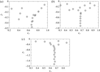
In order to validate the predictions of our numerical procedure for the linear stability analysis, we have made detailed comparisons with several published results for single fluid and core–annular flows. In figure 3, we compare the eigenspectrums for the Hagen–Poiseuille flow obtained using the present code (by setting
 ${\it\delta}=1$
and
 $R_{s}=R_{f}=0$
) with those given in Schmid & Henningson (Reference Schmid and Henningson2001) for different values of wavenumbers in the axial and the azimuthal directions and find excellent agreement. Note that we use the average velocity as a characteristic scale, rather than the centreline velocity which was used by Schmid & Henningson (Reference Schmid and Henningson2001). The present Reynolds number and phase speed are related with those of Schmid & Henningson (Reference Schmid and Henningson2001) (designated by subscript SH) as
 $Re=2Re_{SH}$
and
 $c=2c_{SH}$
. Excellent agreement is also found (not shown) with the stability analysis of SC core–annular flow through a straight pipe by Selvam et al. (Reference Selvam, Merk, Govindarajan and Meiburg2007). The results obtained in the configurations which are stable in the context of equivalent SC flows, as reported by Selvam et al. (Reference Selvam, Merk, Govindarajan and Meiburg2007), but are unstable in the presence of DD effect, are discussed below.
Comparison of eigenspectrums for the Hagen–Poiseuille flow obtained using the present code (circles) with those given in Schmid & Henningson (Reference Schmid and Henningson2001) (plus signs) for
 $Re_{SH}=2000$
. (a)
 ${\it\alpha}=1$
,
 ${\it\beta}=0$
, (b)
 ${\it\alpha}=0.5$
,
 ${\it\beta}=1$
, and (c)
 ${\it\alpha}=0.25$
,
 ${\it\beta}=2$
. Here
 $Re_{SH}\equiv U_{c}{\it\rho}R/{\it\mu}$
, where
 $U_{c}$
is the centreline velocity and
 ${\it\mu}\;({\it\mu}_{1}={\it\mu}_{2})$
is viscosity of fluid, obtained by setting
 $R_{s}=R_{f}=0$
.

3. Results from the linear stability analysis
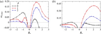
In order to contrast the instability characteristics due to the double-diffusive effect with the equivalent SC system, the variation of maximum growth rate,
 ${\it\omega}_{i,max}$
with increasing viscosity ratio (increasing the value of
 $R_{s}$
) for an SC system (
 ${\it\delta}=1$
and
 $R_{f}=0$
) is presented in figures 4(a) and 4(b) for
 $R_{1}=0.7$
and 0.45, respectively. The rest of the parameter values are
 $Re=1000$
,
 $Sc=10$
and
 $q=0.1$
. Three values of azimuthal wavenumber of the perturbation, i.e.
 ${\it\beta}=0$
, 1 and 2 are considered for the presentation. The higher modes (
 ${\it\beta}>2$
) are found to be stable for the parameters considered in this study. Here,
 $R_{s}>0$
 $({<}0)$
represents a situation when the annular fluid is more (less) viscous than the core fluid. It can be seen in figure 4(a) for
 $R_{1}=0.7$
that when
 $R_{s}>0$
, i.e.
 ${\it\mu}_{2}>{\it\mu}_{1}$
,
 ${\it\beta}=1$
is the most unstable mode giving the highest growth rate, whereas the axisymmetric mode
 $({\it\beta}=0)$
is the least unstable one;
 ${\it\beta}=2$
is the intermediate unstable mode for the parameter values considered. A similar observation can be made for
 $R_{1}=0.45$
(figure 4
b). For
 $R_{s}<0$
, when the annular fluid is less viscous than the core fluid (
 ${\it\mu}_{2}<{\it\mu}_{1}$
), the axisymmetric mode
 $({\it\beta}=0)$
and swirling mode with
 ${\it\beta}=1$
give almost the same maximum growth rate up to
 $R_{s}\sim -0.5$
, but the axisymmetric mode dominates for
 $R_{s}<-0.5$
. A similar conclusion was reported by Selvam et al. (Reference Selvam, Merk, Govindarajan and Meiburg2007). In figure 4(b) it can be seen that moving the mixed layer closer to the centreline
 $(R_{1}=0.45)$
significantly increases the maximum growth rate for a positive viscosity ratio
 $(R_{s}>0)$
, but decreases the maximum growth rate for a negative viscosity ratio
 $(R_{s}<0)$
; in fact, unlike
 $R_{1}=0.7$
(figure 4
a), for
 $R_{1}=0.45$
the flow is stable for
 $R_{s}<0$
for this set of parameter values. In the discussion to follow, the linear instability characteristics due to the DD effect (
 ${\it\delta}>1$
) in the parameter regimes where the equivalent SC flow is stable are investigated. In the rest of the work, only the axisymmetric
 $({\it\beta}=0)$
and corkscrew
 $({\it\beta}=1)$
modes are considered as higher modes
 $({\it\beta}>1)$
are less unstable or even stable.
Variation of the maximum growth rate,
 ${\it\omega}_{i,max}$
versus
 $R_{s}$
for different values of
 ${\it\beta}$
in an SC system (
 ${\it\delta}=1$
and
 $R_{f}=0$
): (a)
 $R_{1}=0.7$
and (b)
 $R_{1}=0.45$
. The rest of the parameter values are
 $Re=1000$
,
 $Sc=10$
and
 $q=0.1$
.

3.1. Effect of
 ${\it\delta}$

The influence of varying the diffusivity ratio of the faster-diffusing scalar to that of the slower-diffusing scalar,
 ${\it\delta}$
is investigated in figure 5(a,b) for
 $R_{s}=1$
,
 $R_{f}=-1.1$
and
 $R_{s}=-1.1$
,
 $R_{f}=1$
, respectively. The remaining parameter values are
 $Re=1000$
,
 $Sc=10$
,
 $R_{1}=0.7$
,
 $q=0.1$
and
 ${\it\beta}=1$
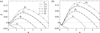
. From figure 4(a), it can be seen that the parameters considered in figure 5(a) correspond to a situation when the slower-diffusing scalar has a destabilising influence, whereas the faster-diffusing scalar is close to a neutrally stable state. The situation is opposite in figure 5(b), wherein the faster-diffusing scalar has a destabilising influence, whereas the slower-diffusing scalar is close to a neutrally stable state. In both the cases, as
 $R_{s}+R_{f}=-0.1$
, the net stratification is stabilizing. The equivalent SC system whose diffusivity is the average of
 $\mathscr{D}_{s}$
and
 $\mathscr{D}_{f}$
, is stable for the parameter values considered. However, the flow becomes unstable in the presence of the DD effect. It can be seen in figure 5(a) that the growth rate,
 ${\it\omega}_{i}$
, becomes positive for
 ${\it\delta}=5$
, which indicates temporal instability. We also observe that increasing
 ${\it\delta}$
increases the growth rate.
Inspection of figure 5(b) reveals that the flow becomes unstable for
 ${\it\delta}=2.5$
; a
 ${\it\delta}$
value lower than that observed in figure 5(a). This is counter-intuitive. In figure 5(a), one observes that the scalar
 $f$
will diffuse away faster, leaving the destabilizing effect of the scalar
 $s$
, which causes the DD instability. Intuitively less obvious is the existence of the DD instability in figure 5(b), where the faster-diffusing scalar is destabilizing and the slower-diffusing scalar is stabilizing. In this case, the scalar having a destabilising influence will diffuse away faster, leaving the stabilising scalar in the flow system. The instabilities seen in figure 5(a,b) are broadly analogous to the fingering and the oscillatory instabilities, respectively in the DD convection of gravity-driven systems (Turner Reference Turner1974).
Effect of the relative diffusion rate,
 ${\it\delta}$
on the instability growth rate for (a)
 $R_{s}=1$
,
 $R_{f}=-1.1$
, and (b)
 $R_{s}=-1.1$
,
 $R_{f}=1$
. The rest of the parameter values are
 $Re=1000$
,
 $Sc=10$
,
 $R_{1}=0.7$
,
 $q=0.1$
and
 ${\it\beta}=1$
. The equivalent SC flow (
 $Sc_{eq}=2Sc/({\it\delta}+1)$
,
 $R_{s}=-0.1$
and
 $R_{f}=0$
) is stable
 $({\it\omega}_{i}<0)$
for these sets of parameter values. The points
 $A_{1}$
,
 $B_{1}$
,
 $C_{1}$
and
 $D_{1}$
in (a) correspond to
 ${\it\alpha}=1$
, 1.5, 1.8 and 2, respectively. The points
 $A_{2}$
,
 $B_{2}$
,
 $C_{2}$
and
 $D_{2}$
in (b) correspond to
 ${\it\alpha}=1.54$
, 1.87, 2.14 and 2.4, respectively.

In order to gain insight into the mechanisms underlying the instability which arises due to the DD effect discussed in the foregoing, we carried out an analysis of the energy budget (Selvam et al. Reference Selvam, Merk, Govindarajan and Meiburg2007; Sahu et al. Reference Sahu, Ding, Valluri and Matar2009) and an inviscid stability analysis (Sahu & Govindarajan Reference Sahu and Govindarajan2005), which are outlined in appendices A and B, respectively.
Energy budgets for the points labelled
 $A_{1}$
,
 $B_{1}$
,
 $C_{1}$
and
 $D_{1}$
in figure 5(a).

In the energy budget analysis, the temporal rate of change of the perturbation kinetic energy,
 $\dot{\mathscr{E}}$
is split into several terms based on their contributions to influence
 $\dot{\mathscr{E}}$
, namely, the rate of transfer of energy from the basic flow to the perturbation (
 $\mathscr{P}$
), rate of viscous dissipation energy of the perturbation (
 $\mathscr{D}$
), the rate of energy of the perturbation due to mean viscosity gradients
 $(\mathscr{A})$
, the rate of perturbation energies associated with the gradient of viscosity perturbation in the radial (
 $\mathscr{B}_{r}$
) and axial
 $(\mathscr{B}_{z})$
directions and the rate of energy due to the gradient of viscosity perturbation (
 $\mathscr{C}$
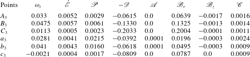
) (see appendix A for details). In table 1, the contributions due to these rate of energy transferred terms at points
 $A_{1}$
,
 $B_{1}$
,
 $C_{1}$
and
 $D_{1}$
in figure 5(a), which correspond to axial wavenumbers at which the growth rates are maximum for
 ${\it\delta}=2.5$
, 5, 10 and 20, respectively, are provided. It can be seen that for
 ${\it\delta}=2.5$
(point
 $A_{1}$
)
 $\dot{\mathscr{E}}$
is negative, indicating that flow is stable. For
 ${\it\delta}\geqslant 5$
, it can be observed that the largest positive contributor to the instability is
 $\mathscr{P}$
. However,
 $\mathscr{B}_{r}$
also contributed to the instability. The perturbation energies associated with mean viscosity gradient
 $(\mathscr{A})$
, perturbation viscosity gradient in the
 $z$
-direction
 $(\mathscr{B}_{z})$
and perturbation viscosity itself
 $(\mathscr{C})$
are small for all values of
 ${\it\delta}$
considered. The viscous dissipation energy
 $\mathscr{D}$
is negative and thus stabilizing. Inspection of table 1 also reveals that increasing
 ${\it\delta}$
increases the positive contributions at much faster rates than the negative contributions.
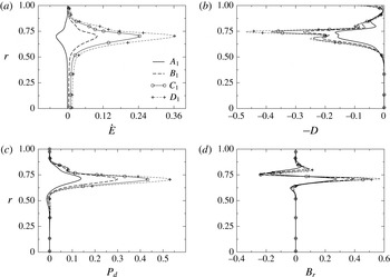
In order to understand this further, the variation of
 ${\dot{E}}$
and the dominant energy terms, i.e.
 $-D$
,
 $P_{d}$
and
 $B_{r}$
(defined in appendix A) of the most dangerous modes (denoted by
 $A_{1}$
 $B_{1}$
,
 $C_{1}$
and
 $D_{1}$
in figure 5
a) in the wall-normal direction are plotted for different values of
 ${\it\delta}$
in figures 6(a), 6(b), 6(c), 6(d), respectively. It can be seen that the rate of production due to the transfer of energy from the basic flow to the perturbation (
 $P_{d}$
) and gradient of viscosity perturbation in the radial (
 $B_{r}$
) are zero everywhere, except in the mixed layer (
 $0.7\leqslant r\leqslant 0.8$
). The rate of viscous dissipation
 $(-D)$
, i.e. the rate of energy transfer from the perturbation to the mean flow is negative at the mixed layer and near the pipe wall. However, the combined positive contribution from
 $P_{d}$
and
 $B_{r}$
is more than the negative viscous dissipation for
 ${\it\delta}>2.5$
for this set of parameter values. Thus, for
 ${\it\delta}>2.5$
, the perturbation gains energy from the mean flow, which in turn destabilises the flow.
Radial variations of (a) the rate of change of kinetic energy,
 ${\dot{E}}$
, (b) the dissipation rate; the negative
 $(D)$
is shown to help viewing, (c) the production rate,
 $P_{d}$
and (d)
 $B_{r}$
of the most dangerous modes represented by
 $A_{1}$
 $B_{1}$
,
 $C_{1}$
and
 $D_{1}$
in figure 5(a) for different values of
 ${\it\delta}$
in the wall-normal direction. The rest of the parameter values are the same as those used to generate figure 5(a).

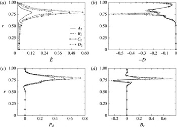
Radial variations of (a) the rate of change of kinetic energy,
 ${\dot{E}}$
, (b) the dissipation rate; the negative
 $(D)$
is shown to help viewing, (c) the production rate,
 $P_{d}$
and (d)
 $B_{r}$
of the most dangerous modes represented by
 $A_{2}$
 $B_{2}$
,
 $C_{2}$
and
 $D_{2}$
in figure 5(b) for different values of
 ${\it\delta}$
in the wall-normal direction. The rest of the parameter values are the same as those used to generate figure 5(b).

Energy budgets for the points labelled
 $A_{2}$
,
 $B_{2}$
,
 $C_{2}$
and
 $D_{2}$
in figure 5(b).

The instability due to the DD effect shown in figure 5(b) is intuitively less obvious as in this case, the faster-diffusing scalar is more destabilizing than the slower-diffusing scalar. Thus, the former will diffuse faster, leaving only the stabilising one (
 $s$
) in the system. It can be seen in table 2 and figure 7 that
 $\dot{\mathscr{E}}$
is positive even for
 ${\it\delta}=2.5$
, making the flow unstable at a lower diffusivity ratio as compared to that in figure 5(a). The contributions from all the energy terms for
 $R_{s}=-1.1$
and
 $R_{f}=1$
are also higher than those obtained for
 $R_{s}=1$
and
 $R_{f}=-1.1$
.
In order to understand the stability behaviour of the flow in the inviscid limit (
 $Re\rightarrow \infty$
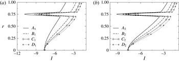
), an inviscid analysis is conducted in appendix B. Based on this, a pipe flow is inviscidly unstable if the inviscid stability function,
 $I\equiv U_{z}^{\prime \prime }-U_{z}^{\prime }({\it\alpha}^{2}r^{2}-{\it\beta}^{2})/r/({\it\alpha}^{2}r^{2}+{\it\beta}^{2})$
corresponding to the most dangerous mode changes its sign inside the domain. The radial variations of the inviscid stability function,
 $I$
for
 $R_{s}=1$
,
 $R_{f}=-1.1$
and
 $R_{s}=-1.1$
,
 $R_{f}=1$
, with the rest of the parameter values the same as those used to generate figure 5, are shown in figure 8(a,b), respectively. It can be seen that for both sets of parameters,
 $I$
remains negative for all values of
 ${\it\delta}$
. In fact, increasing
 ${\it\delta}$
takes away the profile from
 $I=0$
, which implies that the flow is inviscidly stable for these sets of parameters. It has been checked that this is true even for all other cases studied in this work. As the flow is stable in the limit (
 $Re\rightarrow \infty$
), we will see below that the neutral stability curves are closed curves, unlike several other shear flows, e.g. plane Poiseuille flow.
Radial variations of the inviscid instability function,
 $I$
for the most dangerous modes for (a)
 $R_{s}=1$
and
 $R_{f}=-1.1$
, (b)
 $R_{s}=-1.1$
and
 $R_{f}=1$
. The rest of the parameter values are the same as those used to generate figure 5.

(a) The effect of varying
 ${\it\delta}$
on the neutral stability curves (solid lines:
 ${\it\beta}=0$
, dashed lines:
 ${\it\beta}=1$
), (b) zoomed view of (a), and (c)
 $Re_{cr}$
versus
 ${\it\delta}$
for both
 ${\it\beta}$
values. The rest of the parameter values are
 $Sc=10$
,
 $R_{1}=0.45$
,
 $q=0.1$
,
 $R_{s}=1$
and
 $R_{f}=-1.1$
.

Next, we investigate the effect of variation of
 ${\it\delta}$
on the neutral stability curves for both the axisymmetric (
 ${\it\beta}=0$
) and corkscrew modes (
 ${\it\beta}=1$
) in figure 9. The rest of the parameter values are
 $Sc=10$
,
 $R_{1}=0.45$
,
 $q=0.1$
,
 $R_{s}=1$
and
 $R_{f}=-1.1$
. For this figure,
 $R_{1}$
is fixed at
 $0.45$
. This selection is motivated from figure 4(b), which shows that for
 $R_{1}=0.45$
, when
 $R_{s}<0$
, i.e. when the annular fluid is less viscous than the core fluid, the flow is completely stable for all values of
 ${\it\beta}$
. Here, the objective is to demonstrate the appearance of the DD instability in the parameter regime where the equivalent SC flow (whose diffusivity is the average of
 $\mathscr{D}_{s}$
and
 $\mathscr{D}_{f}$
, i.e.
 $Sc_{eq}=2Sc/({\it\delta}+1)$
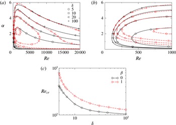
) is stable. In the neutral stability curves shown in figure 9(a), the flow is unstable in the region inside the closed curves. The neutral stability curves are closed curves for all values of
 ${\it\delta}$
, but complete curves are shown only for
 ${\it\delta}=$
5 and 10. It can also be seen that the unstable region also grows with increase in the value of
 ${\it\delta}$
. The zoomed view of figure 9(a) is shown in figure 9(b), which reveals that increasing
 ${\it\delta}$
decreases the critical Reynolds number,
 $Re_{cr}$
(the minimum value of
 $Re$
at which the flow becomes linearly unstable). This is quantified in figure 9(c), which reveals that
 $Re_{cr}$
for the axisymmetric mode
 $({\it\beta}=0)$
is always less than that of the corkscrew mode
 $({\it\beta}=1)$
, i.e. the faster-growing axisymmetric mode is more unstable than the corresponding corkscrew mode, for this set of parameters.
3.2. Effect of the radial location of the mixed layer
The effects of radial location of the mixed layer,
 $R_{1}$
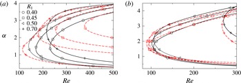
, on the neutral stability curves for the axisymmetric mode (solid lines) and corkscrew mode (dashed lines) are plotted in figure 10(a,b) for
 $R_{s}=1$
,
 $R_{f}=-1.1$
and
 $R_{s}=-1.1$
,
 $R_{f}=1$
, respectively. It can be seen in figure 10(a) that for
 $R_{s}=1$
and
 $R_{f}=-1.1$
, as expected (Selvam et al.
Reference Selvam, Merk, Govindarajan and Meiburg2007), the faster-growing axisymmetric mode is more unstable (lower
 $Re_{cr}$
) than the corresponding corkscrew mode
 $({\it\beta}=1)$
for
 $R_{1}\leqslant 0.5$
. However, interestingly for
 $R_{1}=0.7$
, it can be seen that the faster-growing corkscrew mode
 $({\it\beta}=1)$
becomes more unstable than the axisymmetric mode. It is found that this is due to the overlap of the critical layer (the radial location at which the basic state axial velocity,
 $U_{z}$
is equal to
 $c_{r}$
of the most dangerous mode) with the mixed layer when
 ${\it\beta}=1$
. As discussed by Govindarajan (Reference Govindarajan2004), Talon & Meiburg (Reference Talon and Meiburg2011) for planar flows, the most unstable mode resembles with the interfacial mode of a sharp interface (Yih Reference Yih1967) in this overlap region. Close inspection also reveals that taking the mixed layer closer to the wall destabilises the flow for
 $R_{s}=1$
,
 $R_{f}=-1.1$
up to
 $R_{1}=0.5$
, but increasing
 $R_{1}$
further stabilises the flow (see figure 10
a). For
 $R_{s}=-1.1$
,
 $R_{f}=1$
, the critical Reynolds number is almost the same till
 $R_{1}=0.5$
, but has a huge stabilization for
 $h=0.7$
(see figure 10
b).
The neutral stability curves for different values of
 $R_{1}$
(solid lines:
 ${\it\beta}=0$
, dashed lines:
 ${\it\beta}=1$
): (a)
 $R_{s}=1$
,
 $R_{f}=-1.1$
, and (b)
 $R_{s}=-1.1$
,
 $R_{f}=1$
. The rest of the parameter values are
 $Sc=10$
,
 $q=0.1$
and
 ${\it\delta}=10$
.

3.3. Effect of
$Sc$
and
$q$


Next, the effects of Schmidt number,
 $Sc$
of the slower-diffusing scalar and mixed-layer thickness,
 $q$
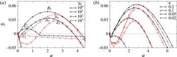
are investigated in figure 11(a,b), respectively. Unlike the DD instability in planar flow (Sahu & Govindarajan Reference Sahu and Govindarajan2011), Schmidt number has a non-monotonic effect in pipe flow for the parameter values considered in this study. A similar behaviour of
 $Sc$
was previously observed in a two-layer planar SC flow for high viscosity ratio in the Stokes flow regime (Talon & Meiburg Reference Talon and Meiburg2011). They also suggested a mechanism of this non-monotonic behaviour of
 $Sc$
using an argument similar to the one proposed by Hinch (Reference Hinch1984) for interfacial flows. It can be seen that increasing
 $Sc$
increases the maximum growth rate of the perturbation and also increases the range of
 ${\it\alpha}$
for which the flow is unstable for both the axisymmetric and corkscrew modes. It can also be seen that for all values of
 $Sc$
, the faster-growing axisymmetric mode is more unstable than the corresponding corkscrew mode. As expected, in figure 11(b), it is found that decreasing the mixed-layer thickness,
 $q$
increases the growth rate.
The effect of varying (a)
 $Sc$
for
 $q=0.1$
, and (b)
 $q$
for
 $Sc=10$
, on the dispersion curves (
 ${\it\omega}_{i}$
versus
 ${\it\alpha}$
). Here solid and dashed lines represent the results for
 ${\it\beta}=0$
and
 ${\it\beta}=1$
, respectively. The radius of the centre of the mixed region, i.e.
 $R_{1}+q/2$
is fixed at 0.5. The rest of the parameter values are
 $Re=500$
,
 $R_{s}=1$
,
 $R_{f}=-1.1$
and
 ${\it\delta}=10$
. The region above the dotted line (
 ${\it\omega}_{i}=0$
) is the unstable region. The points
 $A_{3}$
,
 $B_{3}$
,
 $C_{3}$
and
 $a_{3}$
,
 $b_{3}$
,
 $c_{3}$
in panel (a) correspond to the most dangerous axisymmetric and corkscrew modes for
 $Sc=10$
, 100 and 1000, respectively. The equivalent SC flows (
 $Sc_{eq}=2Sc/({\it\delta}+1)$
,
 $R_{s}=-0.1$
and
 $R_{f}=0$
) are stable
 $({\it\omega}_{i}<0)$
for these sets of parameter values.

It is to be noted here that for the parameter values considered so far, the equivalent single component system whose diffusivity is the average of
 $\mathscr{D}_{s}$
and
 $\mathscr{D}_{f}$
, i.e.
 $Sc_{eq}=2Sc/({\it\delta}+1)$
is linearly stable.
To understand the non-monotonic behaviour of Schmidt number in the DD system, the energy budget analysis is conducted. The contributions of the various energy terms (discussed in the appendix A) at points
 $A_{3}$
,
 $B_{3}$
and
 $C_{3}$
(associated with the most dangerous axisymmetric modes for
 $Sc=10$
, 100 and 1000, respectively) and
 $a_{3}$
,
 $b_{3}$
and
 $c_{3}$
(associated with the most dangerous corkscrew modes for
 $Sc=10$
, 100 and 1000, respectively) are given in table 3. It can be seen that for the axisymmetric modes, the negative contribution due to the viscous dissipation
 $(-\mathscr{D})$
almost balances out the positive contribution due to the gradient of viscosity perturbation in the radial direction
 $\mathscr{B}_{r}$
, and the non-monotonicity in the stability behaviour is clearly due to the rate of transfer of energy from the basic flow to the perturbation (
 $\mathscr{P}$
). However, for the corkscrew mode, the mechanism of instability is due to the combined effects of the energy terms. It can also be seen that the values of
 $\mathscr{B}_{r}$
for axisymmetric modes are much larger than those for the corresponding corkscrew modes. Thus, the faster-growing axisymmetric modes are more unstable then the corresponding corkscrew modes for this set of parameter values. Finally in this section, the effect of the DD phenomenon on unstable configurations in the context of SC flows, will be investigated.
Stability characteristics in the unstable SC regions: (a,c)
 $R_{s}+R_{f}>0$
, (b,d)
 $R_{s}+R_{f}<0$
. The solid and dashed lines represent the results for the DD and the equivalent
 $SC$
systems, respectively. For the DD system in (a)
 $R_{f}=-1$
,
 ${\it\beta}=1$
, and in (b)
 $R_{s}=1$
and
 ${\it\beta}=0$
, and for the single component system (
 $Sc_{eq}=2Sc/({\it\delta}+1)$
, modified
 $R_{s}$
and
 $R_{f}$
values are set to
 $R_{s}+R_{f}$
and
 $R_{f}=0$
), respectively. The rest of the parameter values are
 $R_{1}=0.45$
,
 $q=0.1$
and
 ${\it\delta}=10$
.

Energy budgets for the points labelled
 $A_{3}$
,
 $B_{3}$
,
 $C_{3}$
,
 $a_{3}$
,
 $b_{3}$
and
 $c_{2}$
in figure 11(a).

3.4. Unstable case in the context of SC flows
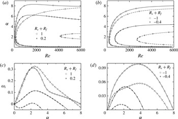
The stability behaviour of the DD systems in the unstable regions for which the net viscosity stratifications are positive (
 $R_{s}+R_{f}>0$
, i.e. when the annular fluid is more viscous than the core fluid) and negative (
 $R_{s}+R_{f}<0$
, i.e. when the annular fluid is less viscous than the core fluid) is investigated in figure 12. As discussed above, the axisymmetric mode is dominant for
 $R_{s}+R_{f}<0$
, whereas the corkscrew mode is the most unstable one for
 $R_{s}+R_{f}>0$
. The corresponding results for the equivalent SC system (
 $Sc_{eq}=2Sc/({\it\delta}+1)$
, where modified
 $R_{s}$
and
 $R_{f}$
values are set to
 $R_{s}+R_{f}$
and
 $R_{f}=0$
) are also shown by dashed lines. It can be seen that the region of instability and the maximum temporal growth rate are larger in the case of the DD system as compared to the equivalent SC system. The critical Reynolds number obtained for the DD system is also lower than that of the equivalent SC system. This result also demonstrates that the DD effect enhances the instability even in the linearly unstable regions in the context of SC flows.
The results presented so far are obtained from the linear stability analysis. The DD flow in the nonlinear region is discussed in the next section.
4. Direct numerical simulations
As axisymmetric modes are found to be the most unstable eigenmodes by the linear stability analysis, in this section, axisymmetric numerical simulations are conducted by solving (2.7)–(2.10) directly without further assumptions using the no-slip and the no-penetration boundary conditions for the velocity components and the no-flux conditions for the scalars
 $s$
and
 $f$
at the pipe wall. A periodic boundary condition is implemented in the axial direction. A bespoke finite-volume flow solver (Sahu et al.
Reference Sahu, Ding, Valluri and Matar2009; Tripathi, Sahu & Govindarajan Reference Tripathi, Sahu and Govindarajan2015) is used to solve the governing equations on a staggered grid. The scalar variables (the pressure and the volume fraction of the outer fluid) are defined at the cell centres and the velocity components are defined at the cell faces, respectively. In order to achieve second-order accuracy, the Adams–Bashforth and the Crank–Nicholson methods are used to discretize the advective and dissipation terms in (2.8), respectively.
The discretized governing equations are given by:
 $$\begin{eqnarray}\displaystyle \frac{\boldsymbol{u}^{\ast }-\boldsymbol{u}^{n}}{{\rm\Delta}t}=\frac{1}{p^{n+1/2}}\left\{-\left[\frac{3}{2}\mathscr{H}(\boldsymbol{u}^{n})-\frac{1}{2}\mathscr{H}(\boldsymbol{u}^{n-1})\right]+\,\frac{1}{2Re}[\mathscr{L}(\boldsymbol{u}^{\ast },{\it\mu}^{n+1})+\mathscr{L}(\boldsymbol{u}^{n},{\it\mu}^{n})]\right\}\!, & & \displaystyle \nonumber\\ \displaystyle & & \displaystyle\end{eqnarray}$$
where
 $\boldsymbol{u}^{\ast }$
is the intermediate velocity, and
 $\mathscr{H}$
and
 $\mathscr{L}$
denote the discrete convection and diffusion operators, respectively.
 ${\rm\Delta}t=t^{n+1}-t^{n}$
and the superscript
 $n$
signifies the discretized
 $n$
th step.
The intermediate velocity
 $\boldsymbol{u}^{\ast }$
is then corrected to
 $(n+1)$
th time level:
 $$\begin{eqnarray}\frac{\boldsymbol{u}^{n+1}-\boldsymbol{u}^{\ast }}{{\rm\Delta}t}=\boldsymbol{{\rm\nabla}}p^{n+1/2}.\end{eqnarray}$$
The pressure distribution is obtained from the continuity equation at time step
 $n+1$
using
 $$\begin{eqnarray}\boldsymbol{{\rm\nabla}}\boldsymbol{\cdot }(\boldsymbol{{\rm\nabla}}p^{n+1/2})=\frac{\boldsymbol{{\rm\nabla}}\boldsymbol{\cdot }\boldsymbol{u}^{\ast }}{{\rm\Delta}t}.\end{eqnarray}$$
The discretized diffusion equations of the slower- and faster-diffusing species are
 $$\begin{eqnarray}\displaystyle & \displaystyle \frac{\frac{3}{2}s^{n+1}-2s^{n}+\frac{1}{2}s^{n-1}}{{\rm\Delta}t}=\frac{1}{Re\,Sc}{\rm\nabla}^{2}s^{n+1}-2\boldsymbol{{\rm\nabla}}\boldsymbol{\cdot }(\boldsymbol{u}^{n}s^{n})+\boldsymbol{{\rm\nabla}}\boldsymbol{\cdot }(\boldsymbol{u}^{n-1}s^{n-1}), & \displaystyle\end{eqnarray}$$
 $$\begin{eqnarray}\displaystyle & \displaystyle \frac{\frac{3}{2}f^{n+1}-2f^{n}+\frac{1}{2}f^{n-1}}{{\rm\Delta}t}=\frac{{\it\delta}}{Re\,Sc}{\rm\nabla}^{2}f^{n+1}-2\boldsymbol{{\rm\nabla}}\boldsymbol{\cdot }(\boldsymbol{u}^{n}f^{n})+\boldsymbol{{\rm\nabla}}\boldsymbol{\cdot }(\boldsymbol{u}^{n-1}f^{n-1}), & \displaystyle\end{eqnarray}$$
The spatio-temporal evolutions of the
 $s$
contours: (a,c,e,g)
 ${\it\delta}=1$
and (b,d,f,h)
 ${\it\delta}=20$
. From top to bottom:
 $t=100$
, 150, 200 and 250. The rest of the parameter values are
 $Re=1000$
,
 $Sc=100$
,
 $R_{s}=1$
,
 $R_{f}=-1.1$
. The values of
 $R_{1}$
and
 $q$
at the starting of the simulations are
 $0.6$
and
 $0.1$
, respectively.

The results obtained from this solver are validated against another finite-volume open source code, Gerris (Popinet Reference Popinet2003; Tripathi et al.
Reference Tripathi, Sahu and Govindarajan2015) with dynamic adaptive grid refinement feature based on the vorticity magnitude and species concentration. We found that the finest grid size of 0.015 (approximately) in the diffusive region of the slower- and faster-diffusing species and grids of size
 $0.06$
(approximately) in the vortical region are sufficient to yield grid independent results to capture the onset of instability and other flow features for the parameters considered in the present study. The readers are referred to Tripathi et al. (Reference Tripathi, Sahu and Govindarajan2015) for a detailed description of the numerical method used in this study.
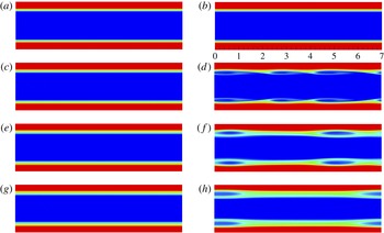
The objective of this section is to demonstrate the appearance of DD instability in the nonlinear regime for
 ${\it\delta}>1$
. It can be seen in figure 13 that the flow is unstable giving rise to ‘roll-up’ structures (Kelvin–Helmholtz (KH) type instability) in the presence of DD effect (
 ${\it\delta}=20$
), whereas the flow is completely stable for
 ${\it\delta}=1$
. The rest of the parameter values are
 $Re=1000$
,
 $Sc=100$
,
 $R_{s}=1$
,
 $R_{f}=-1.1$
 $R_{1}=0.6$
and
 $q=0.1$
. It can be see that for
 $t\geqslant 200$
, a new type of instability of an elliptical shape is observed, which migrates at a speed close to the phase speed of the most dangerous mode for this set of parameters. It is found (not shown) that although at
 $t=0$
the less (high) viscous fluid occupies the annular (core) region of the pipe, the double-diffusive phenomenon alters the viscosity variation at the later times by creating a highly-viscous region near the wall, which is the main cause of instability observed in this case. A similar mechanism was previously observed by Mishra et al. (Reference Mishra, De Wit and Sahu2012) and Bhagat et al. (Reference Bhagat, Tripathi and Sahu2016) in the numerical simulations of displacement flows in planar channel and axisymmetric pipe in the presence of DD effect. On the other hand, the dynamics for
 ${\it\delta}=1$
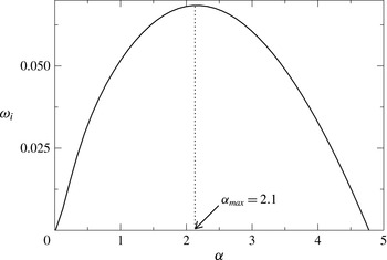
is dominated only by diffusive mixing. The wavelength
 $(2{\rm\pi}/{\it\alpha})$
of the most dangerous mode obtained from the linear stability analysis (shown in figure 14) is approximately equal to that obtained in the nonlinear simulation for
 ${\it\delta}=20$
. This also confirms the finding of the linear stability analysis conducted in the previous section.
The dispersion curve obtained from the linear stability analysis for
 ${\it\delta}=20$
with the rest of the parameters the same as those used to generate figure 13. The phase speed of the most dangerous mode,
 $c_{r}\,(\equiv {\it\omega}_{r\,max}/{\it\alpha}_{max})=1.26$
.

5. Concluding remarks
The instability due to the double-diffusive effect in a core–annular pipe flow of two miscible fluids of the same densities, but different viscosities is investigated using linear stability theory and direct numerical simulations. The DD flow exhibits strikingly different stability characteristics as compared to the DD flow in a planar channel and the corresponding SC flow in a cylindrical pipe. The flow which is stable in the context of SC systems, now becomes unstable in the presence of two scalars diffusing at different rates. It is found that increasing the diffusivity ratio of the faster- and the slower-diffusing scalars enhances the instability by increasing the growth rate of the perturbation, and also by widening the unstable region. In contrast with the single fluid flow through a pipe (Hagen–Poiseuille flow), it is shown that the faster growing axisymmetric mode is more unstable than the corresponding corkscrew mode for the parameter values considered. The equivalent SC flows are stable to all the modes (for any value of
 ${\it\beta}$
). However, this finding is consistent with that of Selvam et al. (Reference Selvam, Merk, Govindarajan and Meiburg2007) for SC core–annular flow, who found that beyond a critical viscosity ratio, when the annular fluid is less viscous than the core fluid, the axisymmetric mode is the most unstable one. It is found that Schmidt number
 $(Sc)$
and the radial location of the mixed layer
 $(R_{1})$
have non-monotonic influences on the instability characteristics, and as expected, decreasing the mixed-layer thickness increases the growth rate.
An energy budget analysis is conducted in order to understand the underlying mechanism of the instability in the DD flow, whose equivalent SC system is stable. It is found that the ‘Reynolds stress’ term, which represents the rate of transfer of energy from the basic flow to the perturbations and rate of energy associated with the gradient of viscosity perturbations in the radial direction provide positive contributions to the DD instability observed in this work. The inviscid stability theory conducted in this study shows that the DD flows in a cylindrical pipe are inviscidly stable. Thus, the neutral stability curves are closed curves at high
 $Re$
.
The direct numerical simulations conducted for different diffusivity ratios,
 ${\it\delta}$
, show the development of the DD instabilities in the nonlinear regime. The behaviour observed in direct numerical simulations is consistent with that obtained from the linear stability theory; the wavelengths of the unstable waves observed in the numerical simulation and the linear stability theory are found to be approximately the same. A new type of instability pattern of an elliptical shape is observed in the nonlinear simulations in the presence of double-diffusive effect. In some flows, such as flow in vertical pipes and in configurations where inertial force is much larger than the gravitational force, buoyancy variations could be negligible, and the present study will be directly relevant to such situations. However, including the density variation will make the problem more complex due to the simultaneous interplay between the viscosity and density stratifications. It is hoped that the present work will motivate experiments on double-diffusive systems with viscosity stratification to confirm the findings.
Acknowledgements
The author gratefully acknowledged Professor M. Deepa of IIT Hyderabad for reading the manuscript and providing valuable suggestions. I also thank Dr M. Tripathi for his help in nonlinear simulations using Gerris.
Appendix A. Energy budget analysis
In order to gain insight into the mechanisms underlying the instabilities, we have carried out an energy budget analysis; a similar analysis was also performed by Selvam et al. (Reference Selvam, Merk, Govindarajan and Meiburg2007) and Sahu et al. (Reference Sahu, Ding, Valluri and Matar2009) for single-component miscible flows in a pipe and a two-dimensional channel, respectively. The energy equation is derived by multiplying (2.18), (2.19) and (2.20) with the radial, azimuthal and axial components of the perturbation velocity, respectively. By adding the resulting equations and integrating across the domain, we obtain the require energy budget equation, given by
 $$\begin{eqnarray}\dot{\mathscr{E}}=\mathscr{P}-\mathscr{D}+\mathscr{A}+\mathscr{B}+\mathscr{C},\end{eqnarray}$$
where
 $$\begin{eqnarray}\displaystyle & \displaystyle \dot{\mathscr{E}}=\int _{0}^{1}{\dot{E}}r\,\text{d}r={\it\omega}_{i}\int _{0}^{1}(u_{r}u_{r}^{\ast }+u_{{\it\theta}}u_{{\it\theta}}^{\ast }+u_{z}u_{z}^{\ast })r\,\text{d}r, & \displaystyle\end{eqnarray}$$
 $$\begin{eqnarray}\displaystyle & \displaystyle \mathscr{P}=\int _{0}^{1}P_{d}r\,\text{d}r=\int _{0}^{1}\text{Im}(u_{r}u_{z}^{\ast })U_{z}^{\prime }r\,\text{d}r, & \displaystyle\end{eqnarray}$$
 $$\begin{eqnarray}\displaystyle \mathscr{D}=\int _{0}^{1}\text{D}r\,\text{d}r & = & \displaystyle \frac{1}{Re}\int _{0}^{1}{\it\mu}_{0}\left[\vphantom{\frac{r^{2}}{1}}u_{r}^{\prime }{u_{r}^{\prime }}^{\ast }+u_{{\it\theta}}^{\prime }{u_{{\it\theta}}^{\prime }}^{\ast }+u_{z}^{\prime }{u_{z}^{\prime }}^{\ast }\right.+\left(\frac{{\it\beta}^{2}}{r^{2}}+{\it\alpha}^{2}\right)(u_{r}u_{r}^{\ast }+u_{{\it\theta}}u_{{\it\theta}}^{\ast }+u_{z}u_{z}^{\ast })\nonumber\\ \displaystyle & & \displaystyle \left.+\,\frac{1}{r^{2}}\{u_{r}u_{r}^{\ast }+u_{{\it\theta}}u_{{\it\theta}}^{\ast }+4{\it\beta}\text{Re}(u_{{\it\theta}}u_{r}^{\ast })\}\right]r\,\text{d}r,\end{eqnarray}$$
 $$\begin{eqnarray}\mathscr{A}=\int _{0}^{1}Ar\,\text{d}r=\frac{1}{Re}\int _{0}^{1}\frac{{\it\mu}_{0}^{\prime }}{r}\left(\frac{\text{d}}{\text{d}r}(ru_{r}u_{r}^{\ast })-u_{{\it\theta}}u_{{\it\theta}}^{\ast }\right)r\,\text{d}r,\end{eqnarray}$$
 $$\begin{eqnarray}\displaystyle \mathscr{B}=\mathscr{B}_{r}+\mathscr{B}_{z} & = & \displaystyle \int _{0}^{1}B_{r}r\,\text{d}r+\int _{0}^{1}B_{z}r\,\text{d}r\nonumber\\ \displaystyle & = & \displaystyle \frac{1}{Re}\int _{0}^{1}U_{z}^{\prime }\text{Re}({\it\mu}^{\prime }z^{\ast })r\,\text{d}r+\frac{1}{Re}\int _{0}^{1}U_{z}^{\prime }\text{Re}({\it\alpha}{\it\mu}u_{r}^{\ast })r\,\text{d}r,\end{eqnarray}$$
 $$\begin{eqnarray}\displaystyle & \displaystyle \mathscr{C}=\int _{0}^{1}Cr\,\text{d}r=\frac{\text{d}P}{\text{d}z}\int _{0}^{1}\text{Re}({\it\mu}u_{z}^{\ast })r\,\text{d}r. & \displaystyle\end{eqnarray}$$
Here
 $\dot{\mathscr{E}}$
represents the temporal rate of change of the perturbation kinetic energy (for unstable flows,
 $\dot{\mathscr{E}}$
is positive);
 $\mathscr{P}$
denotes the ‘Reynolds stress’ term, which determines the rate of transfer of energy from the basic flow to the perturbations and
 $\mathscr{D}$
corresponds to the viscous dissipation of energy of the perturbation. The term
 $\mathscr{A}$
denotes the energy of the perturbations due to mean viscosity gradients. The terms
 $\mathscr{B}$
and
 $\mathscr{C}$
are the perturbation energies due to the gradient of viscosity perturbations and viscosity perturbations, respectively. The term
 $\mathscr{B}$
can be further decomposed into
 ${\mathcal{B}}_{r}$
and
 $\mathscr{B}_{z}$
, where
 $\mathscr{B}_{r}$
and
 $\mathscr{B}_{z}$
are the perturbation energies associated with the gradient of viscosity perturbations in the radial and axial directions, respectively.
Appendix B. Inviscid stability analysis
The necessary conditions for instability in the inviscid limit (
 $Re\rightarrow \infty$
) states that it is necessary to have a point of inflection in the velocity profile for the two-dimensional flow to be inviscidly unstable. This is known as the Rayleigh theorem for inviscid instability in a two-dimensional channel (Rayleigh Reference Rayleigh1880). The corresponding condition for a pipe flow can be derived from (2.17)–(2.20) in the limit
 $Re\rightarrow \infty$
(Sahu & Govindarajan Reference Sahu and Govindarajan2005). The stability equations (2.17)–(2.20) in the cylindrical coordinate systems in the limit
 $Re\rightarrow \infty$
are given by
 $$\begin{eqnarray}\displaystyle & \displaystyle {\it\alpha}u_{z}+u_{r}^{\prime }+\frac{u_{r}}{r}+\frac{1}{r}{\it\beta}u_{{\it\theta}}=0, & \displaystyle\end{eqnarray}$$
 $$\begin{eqnarray}\displaystyle & \displaystyle -{\it\alpha}cu_{r}+U_{z}{\it\alpha}u_{r}=-p^{\prime }, & \displaystyle\end{eqnarray}$$
 $$\begin{eqnarray}\displaystyle & \displaystyle -{\it\alpha}cu_{{\it\theta}}+U_{z}{\it\alpha}u_{{\it\theta}}=-\frac{{\it\beta}p}{r}, & \displaystyle\end{eqnarray}$$
 $$\begin{eqnarray}\displaystyle & \displaystyle -{\it\alpha}cu_{z}+U_{z}{\it\alpha}u_{z}+u_{r}U_{z}^{\prime }=-p{\it\alpha}. & \displaystyle\end{eqnarray}$$
 $u_{{\it\theta}}$
,
 $u_{z}$
and
 $p$
from the above equations, we obtain
 $$\begin{eqnarray}\displaystyle & & \displaystyle (U_{z}-c)\left[u_{r}^{\prime \prime }+\frac{(3{\it\beta}^{2}+{\it\alpha}^{2}r^{2})}{({\it\alpha}^{2}r^{2}+{\it\beta}^{2})}\frac{u_{r}^{\prime }}{r}-\frac{({\it\alpha}^{2}r^{2}+{\it\beta}^{2}+2)}{({\it\alpha}^{2}r^{2}+{\it\beta}^{2})}{\it\alpha}^{2}u_{r}+(1-{\it\beta}^{2})\frac{u_{r}}{r^{2}}\right]\nonumber\\ \displaystyle & & \displaystyle \qquad \qquad \qquad -\,\left[U_{z}^{\prime \prime }-\frac{({\it\alpha}^{2}r^{2}-{\it\beta}^{2})}{r({\it\alpha}^{2}r^{2}+{\it\beta}^{2})}U_{z}^{\prime }\right]u_{r}=0.\end{eqnarray}$$
Let us define a function
 $f(r)$
, which is given by
 $$\begin{eqnarray}\frac{f^{\prime }}{f}=\left[\frac{3{\it\beta}^{2}+{\it\alpha}^{2}r^{2}}{r({\it\alpha}^{2}r^{2}+{\it\beta}^{2})}\right].\end{eqnarray}$$
Now multiplying (B 5) with
 $f(r)u_{r}^{\ast }$
and integrating from
 $r=0$
to
 $r=1$
, we obtain
 $$\begin{eqnarray}\displaystyle & & \displaystyle \int _{0}^{1}(fu_{r}^{\prime })^{\prime }u_{r}^{\ast }\,\text{d}r-\int _{0}^{1}f\left[\frac{{\it\alpha}^{2}r^{2}+{\it\beta}^{2}+2}{{\it\alpha}^{2}r^{2}+{\it\beta}^{2}}\right]{\it\alpha}^{2}|u_{r}|^{2}\,\text{d}r+\int _{0}^{1}(1-{\it\beta}^{2})\frac{|u_{r}|^{2}}{r^{2}}\,\text{d}r\nonumber\\ \displaystyle & & \displaystyle \quad =\int _{0}^{1}f\left[U_{z}^{\prime \prime }-\frac{{\it\alpha}^{2}r^{2}-{\it\beta}^{2}}{r({\it\alpha}^{2}r^{2}+{\it\beta}^{2})}U_{z}^{\prime }\right]\frac{|u_{r}|^{2}}{|U_{z}-c|^{2}}(U_{z}-c)^{\ast }\,\text{d}r,\end{eqnarray}$$
where, superscript * denotes complex conjugate quantities. Integrating the first term in (B 7) and applying the boundary conditions, we find
 $$\begin{eqnarray}\int _{0}^{1}(fu_{r}^{\prime })^{\prime }u_{r}^{\ast }\,\text{d}r=fu_{r}^{\ast }u_{r}^{\prime }|_{0}^{1}-\int _{0}^{1}f|u_{r}^{\prime }|^{2}\,\text{d}r=-\int _{0}^{1}f|u_{r}^{\prime }|^{2}\,\text{d}r.\end{eqnarray}$$
As
 $f$
is always positive (see (B 6)), it can be shown that for any values of
 ${\it\beta}$
, the left-hand side of (B 7) is real and negative.
Thus, equating the imaginary part of (B 7), we obtain
 $$\begin{eqnarray}c_{i}\int _{0}^{1}f\left[U_{z}^{\prime \prime }-\frac{({\it\alpha}^{2}r^{2}-{\it\beta}^{2})}{r({\it\alpha}^{2}r^{2}+{\it\beta}^{2})}U_{z}^{\prime }\right]\frac{|u_{r}|^{2}}{|U_{z}-c|^{2}}\,\text{d}r=0,\end{eqnarray}$$
where
 $c_{i}$
is the imaginary part of the phase speed,
 $c$
. For unstable flow
 $c_{i}>0$
, hence
 $$\begin{eqnarray}\int _{0}^{1}fI\frac{|u_{r}|^{2}}{|U_{z}-c|^{2}}\,\text{d}r=0,\end{eqnarray}$$
where
 $$\begin{eqnarray}I\equiv U_{z}^{\prime \prime }-\frac{({\it\alpha}^{2}r^{2}-{\it\beta}^{2})}{r({\it\alpha}^{2}r^{2}+{\it\beta}^{2})}U_{z}^{\prime }.\end{eqnarray}$$
Therefore, a necessary condition of instability for pipe flow is the quantity
 $I=0$
at some radial location inside the pipe.
Appendix C. Parallel flow assumption
Consider a situation when a splitter plate is located at
 $z<z_{0}$
, at a constant
 $r$
and the parallel streams of two miscible fluids flow on both sides of this plate. The streams come in to contact with each other at
 $z=z_{0}$
. The two fluids begin to mix with each other for
 $z>z_{0}$
, thus producing a stratified layer. The thickness ‘
 $q$
’ of this layer grows as the fluids move downstream and therefore
 $q$
is a function of
 $z$
.
We know at any location, the mean concentrations
 $f_{0}$
and
 $s_{0}$
corresponding to the species
 $F$
and
 $S$
satisfy
 $$\begin{eqnarray}\displaystyle & \displaystyle \frac{\partial f_{0}}{\partial t}+\boldsymbol{u}\boldsymbol{\cdot }\boldsymbol{{\rm\nabla}}f_{0}=\frac{{\it\delta}}{Re\,Sc}{\rm\nabla}^{2}f_{0}, & \displaystyle\end{eqnarray}$$
 $$\begin{eqnarray}\displaystyle & \displaystyle \frac{\partial s_{0}}{\partial t}+\boldsymbol{u}\boldsymbol{\cdot }\boldsymbol{{\rm\nabla}}s_{0}=\frac{1}{Re\,Sc}{\rm\nabla}^{2}s_{0}, & \displaystyle\end{eqnarray}$$
 $Pe\equiv ReSc$
), we can make the assumption of locally parallel flow (variations of
 $f_{0}$
and
 $s_{0}$
in the
 $r$
direction are much larger than that in the axial direction); thus (
 $u_{r}\ll u_{z}$
and
 $\partial ^{2}/\partial z^{2}\ll \partial ^{2}/\partial r^{2}$
). This is equivalent to saying that the variations of the gradients of the flow variables and the thickness
 $q$
of the mixed region have much larger length scale than the disturbance wavelength. In such a scenario, the concentrations are function of
 $r$
and
 $t$
only and not of
 $z$
. Thus the above equations reduce to
 $$\begin{eqnarray}\frac{\partial f_{0}}{\partial t}=\frac{1}{Pe}\frac{\partial ^{2}f_{0}}{\partial r^{2}},\end{eqnarray}$$
and
 $$\begin{eqnarray}\frac{\partial s_{0}}{\partial t}=\frac{1}{Pe}\frac{\partial ^{2}s_{0}}{\partial r^{2}}.\end{eqnarray}$$
Also, using the same approximation, we know that
 $U\sim O(1)$
,
 $r\sim \sqrt{{\it\nu}}$
, where
 ${\it\nu}$
is the kinematic viscosity. Therefore,
 $qf_{0}\sim O(r^{2})$
since
 $f_{0}$
is the mean concentration over the mixed layer of thickness
 $q$
. This implies that
 $\partial f_{0}/\partial z\simeq (1/q)\,O({\it\delta}/Pe)$
(from (C 3)). Similarly, (from (C 4)), we can get
 $\partial s_{0}/\partial z\simeq (1/q)O(1/Pe)$
. So, for large values of
 $Pe$
,
 $\partial f_{0}/\partial z$
,
 $\partial s_{0}/\partial z$
are very small, showing that the downstream variations of
 $f_{0}$
and
 $s_{0}$
are very small, which in turn implies that the changes in the thickness
 $q$
of the mixed layer along the
 $z$
-direction is very small.
Alternatively, if we assume a similarity solution
 $f_{0}(r/q(z))\simeq f({\it\zeta})$
(where
 ${\it\zeta}=(r/q(z))$
), from (C 1), at the steady state, we obtain
 $$\begin{eqnarray}u_{z}\frac{\text{d}f_{0}}{\text{d}{\it\zeta}}\left(-\frac{{\it\zeta}}{q}\,\frac{\text{d}q}{\text{d}z}\right)\simeq \frac{{\it\delta}}{Pe}\left(\frac{\text{d}^{2}f_{0}}{\text{d}{\it\zeta}^{2}}\,\frac{1}{q^{2}}\right).\end{eqnarray}$$
As a consequence,
 $$\begin{eqnarray}\frac{1}{q}\,\frac{\text{d}q}{\text{d}z}\sim \frac{{\it\delta}}{q^{2}Pe}\Rightarrow \frac{\text{d}q}{\text{d}z}\sim \frac{1}{q}O\left(\frac{{\it\delta}}{Pe}\right).\end{eqnarray}$$
Thus, the downstream growth of mixed layer is inversely proportional to the Péclet number as
 $u_{r}$
and
 ${\it\zeta}$
are of
 $O(1)$
and
 $O(\text{d}f_{0}/\text{d}{\it\zeta})\simeq O(\text{d}^{2}f_{0}/\text{d}{\it\zeta}^{2})$
, which confirms that for the Reynolds and Schmidt numbers considered in the present study, the assumption of uniform thickness of the viscosity stratified layer (mixed layer) is justified.
Now, the solution of (C 3) or (C 4) is an error function, and the fifth-order polynomial is a good representation of this. We also note here that such basic flows are commonly used in stability studies. Several authors have used the same logic to give a basic concentration profile in the form of a hyperbolic tangent (Ern, Charru & Luchini Reference Ern, Charru and Luchini2003) or an error function (e.g. Selvam et al. Reference Selvam, Merk, Govindarajan and Meiburg2007; Talon & Meiburg Reference Talon and Meiburg2011). Some have also used a fifth-order polynomial (see e.g. Malik & Hooper Reference Malik and Hooper2005; Sahu et al. Reference Sahu, Ding, Valluri and Matar2009), which is smooth enough to approximate either profile.