There are two widely accepted but contradictory findings about the agricultural frontier of the nineteenth-century United States. The first is that the population of the frontier was highly geographically mobile.Footnote 1 A large fraction of families observed at one point in time are not observed in the same location five or ten years later. The second is that the economic return to geographic persistence on the frontier was high. The opportunity to accumulate wealth reflected the abundance and rapid price appreciation of land.Footnote 2 These facts are well established but raise a question: if the returns to geographic persistence on the frontier were so high, why was the frontier population so mobile?
Economic models of migration posit that income, wealth, or utility maximization underlies the choice of where to live.Footnote 3 A useful framework for identifying the causes of migration on the frontier is the “push-pull” model. In its simplest form, the model posits that adverse economic developments (e.g., in the form of declining wages, rising unemployment, or poor harvests) can push migrants out of their places of residence, or that economic opportunity (e.g., in the form of rising wages, superior amenities or public goods, or more fertile land) can pull migrants away. More sophisticated forms of the model recognize that migration depends on relative prices and thus push and pull forces jointly determine the incentives for migration.
Which set of factors—push or pull—exerted a greater influence on migration decisions on the frontier? In most histories of the frontier, “push” factors have predominated, as historians have emphasized periodic economic hardships caused by drought, low farm prices, or farm mismanagement.Footnote 4 This article argues, however, that “pull” factors were more important—at least for the decades under study. Economic opportunity was widespread and migrants were pulled elsewhere because of the abundance and rapid price appreciation of frontier land, helping to explain the occurrence of both high rates of wealth accumulation and mobility.
Like earlier studies of geographic mobility on the frontier, this one employs a data set of families linked between the decennial federal censuses. Each family was living in Kansas, Nebraska, or the Dakota Territory in 1870 and is observed in the 1860 and 1870 censuses or the 1860, 1870, and 1880 censuses.Footnote 5 But unlike other studies, this one follows non-persisters after they leave their place of residence, enabling comparisons of post-migration wealth between persisters and non-persisters.
In the first part of the article, I document the greater wealth accumulation of persisters in frontier townships and counties. The wealth of county persisters was nearly 2.5 times higher than that of non-persisters in the 1860s.Footnote 6 Ordinary least squares (OLS) regression analysis shows geographic persistence had a large and positive effect on wealth accumulation between 1860 and 1870, consistent with the accumulation of location-specific human capital and Ricardian rents on land in frontier areas.Footnote 7 The effect of persistence disappears, however, when the persistence decision and wealth accumulation are treated endogenously. Using variation between frontier counties in the incidence of Confederate guerilla raids and attacks during the Civil War to generate exogenous migration, I find the effect of geographic persistence on wealth was zero. The abundance of cheap farmland, rising population densities, and the rapid appreciation of real estate created a steady supply of new opportunities for non-persisters to accumulate wealth.
In the second part of the article, I turn to the causes of mobility and persistence between 1870 and 1880. The frontier population was quite mobile. Only 36 percent of families could be found in the same township in 1870 and 1880. The probability of migration was highest for blue-collar workers, the young, tenants, and the unmarried. These individuals had the largest potential benefit of migration, but also less ability to accumulate wealth than persisters. The large number of young and blue-collar migrants helps to explain both the wealth accumulation of persisters and the high degree of geographic mobility on the frontier.
GEOGRAPHIC MOBILITY ON THE AGRICULTURAL FRONTIER
Typically, researchers interested in geographic mobility have compared the population of a township or county in one census year to the population of the same place in the preceding or subsequent census year.Footnote 8 Families appearing in one census but not the next are classified as non-persisters.
James Malin pioneered this approach in his study of Kansas farmers between 1855 and 1934.Footnote 9 His main finding was that the farm population of Kansas was highly mobile. In eastern Kansas, only 26 percent of farmers could be found in the same township in 1860 and 1870, and only 44 percent between 1870 and 1880. Malin uncovered other interesting patterns, including persistence rates specific to particular locations increased over time, mobility increased during economic downturns, but that the incidence of drought or other environmental adversities (measured by degree of longitude west and changes in the amount of rainfall over time) were not correlated with persistence.Footnote 10 Based on these findings, Malin concluded that the causes of geographic mobility were myriad and complex and “a high degree of persistence or mobility of farm operators does not necessarily mean either prosperity or failure.”Footnote 11
Subsequent studies of other areas show frontier populations in Iowa, Illinois, and Wisconsin exhibited similar tendencies. For instance, Allan Bogue finds persistence rates between 1860 and 1870 in four townships in Iowa ranged between 37 and 56 percent.Footnote 12 Among the factors found to have been positively correlated with persistence on the agricultural frontier were age, wealth, and marital status.Footnote 13
Unanswered Questions
While earlier studies have substantially advanced our knowledge of geographic mobility on the frontier, they have some methodological shortcomings and therefore leave some important questions unanswered. First, as most studies acknowledge, persistence rates reflect factors other than out-migration and thus distort the actual extent of mobility. Absence from the manuscript schedules a decade later could reflect not only out-migration, but also mortality or under-enumeration.Footnote 14 Ignoring mortality or underenumeration imparts a downward bias to persistence rates, although the bias from ignoring mortality in frontier areas is likely to be small because of the youthfulness of the population. Second, existing studies do not observe the post-migration outcomes of non-persisters. Thus, it is not possible to know whether persistence had a positive or negative effect on economic outcomes. Without such information, it is hard to interpret the meaning of non-persistence.
The Data
The indexing of the censuses and advances in data collection methods mean many of the deficiencies of earlier studies can be overcome. In this article, non-persisters and persisters are observed at two points in time and therefore the effect of persistence on outcomes like wealth or occupation can be estimated. Also, mortality will not bias persistence rates downward because persistence is conditional on survival to and enumeration in the next census.Footnote 15
The data for this article were collected as follows.Footnote 16 First, a sample of 7,257 families living in Kansas, Nebraska, or the Dakota Territory (the agricultural frontier) was drawn from the manuscript schedules of the 1870 U.S. Census. These families had uncommon combinations of first and last names (to facilitate the matching of records between the censuses), but were otherwise representative of the frontier population. Then these same families were sought in the manuscript schedules of the 1860 U.S. Census using the census indexes. Families were matched between the censuses on the basis of their Soundex-coded names, ages, and birthplaces. This procedure resulted in the successful matching of 1,271 families residing on the frontier in 1870, but elsewhere in 1860 and 300 families residing on the frontier in both years. The censuses provide information about place of residence (township, county, and state), age, occupation, real estate wealth, personal property wealth, place of birth, and ability to read and write.
Families successfully matched between the 1860 and 1870 censuses were also sought in the 1880 U.S. Census. Employing identical procedures, this step resulted in 684 families linked between the 1860, 1870, and 1880 censuses. Except for wealth, the 1880 census provides the same information as the preceding censuses. Because of this omission, I use the sample of 300 families (of which 276 contain complete information about township of residence and wealth in both years) to estimate the effect of geographic persistence on wealth between 1860 and 1870 and the sample of 684 families to study the causes of persistence between 1870 and 1880. Because of the backward linkage of families from the 1870 to the 1860 census, inclusion in the sample is conditional on residency on the frontier in 1870 and therefore the experiences of families living on the frontier in 1860 but elsewhere in 1870 are not captured.
To analyze geographic persistence, each family in the sample had to be categorized as a persister or non-persister based on information about place of residence in the censuses. Each family was classified as a township persister (same township in both census years), an intra-county mover (same county in both years but different townships), an intercounty mover (different frontier counties in both years), or an interregional mover (living in Kansas, Nebraska, or the Dakota Territory in one census year, but elsewhere a decade later). The classification of families as persisters or non-persisters accounted for changes in the names and boundaries of frontier counties (though not townships) over time. For instance, residents of counties that were subdivided and renamed between the censuses were classified as persisters.
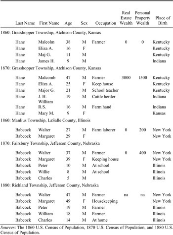
Table 1 shows two observations from the data set and how the persistence definitions were applied. The first is the Hane family, who lived in the same Kansas township in 1860 and 1870 and thus was classified as a township persister. The second is the Babcock family, who lived in Illinois in 1860 and in Nebraska in 1870 and 1880. Because the Babcock family moved between townships in the same county between 1870 and 1880, it was classified as an intra-county mover.
The linked data have several shortcomings. First, the geographic persistence rates in this study are conditional on survival to and enumeration in the next census and thus are not comparable to the unconditional rates reported in most other studies of the frontier.
HANE AND BABCOCK FAMILIES LINKED BETWEEN THE U.S. CENSUSES

Sources:
The 1860 U.S. Census of Population, 1870 U.S. Census of Population, and 1880 U.S. Census of Population.
Another factor confounding comparisons to other studies is the persistence rates in this study pertain to a large number of townships and counties, whereas those in other studies pertain to a single township or county. Idiosyncratic local influences on persistence are therefore averaged out. Further, the time period of study may not be representative. During the Civil War, Kansas counties bordering Missouri were the target of Confederate guerilla attacks that caused widespread out-migration. Moreover, with the exception of a mild and short drought in the early 1860s and the economic downturn of 1873, the 1860s and 1870s were temperate and prosperous years.Footnote 17 In later decades, the farming frontier experienced severe droughts and economic downturns.Footnote 18
THE EFFECT OF GEOGRAPHIC MOBILITY ON WEALTH ACCUMULATION
Our knowledge of the effect of geographic mobility on economic outcomes like income, wealth, and occupation has substantial gaps because historians have been unable to observe the post-migration outcomes of non-persisters. In comparison, we know much more about the effect of geographic precedence on wealth. Previous studies of the frontier have identified an economic return to geographic precedence.Footnote 19 Early arrivers (those appearing in the preceding census) accumulated wealth much faster than latecomers. For instance, Mary Eschelbach Gregson shows half of the early arrival premium was due to the accumulation of location-specific human capital and half was due to the heterogeneity of land and the ability of the first settlers to pick the best parcels.Footnote 20 Geographic precedence and persistence are not the same, but the returns to geographic precedence suggest there were also returns to geographic persistence. Like early arrivers, geographic persisters would have accumulated more knowledge about local agriculture and markets than movers. In this section, I use information about the post-migration wealth of non-persisters in 1870 to estimate the effect of persistence on wealth accumulation.
Geographic Mobility and Wealth Accumulation, 1860–1870
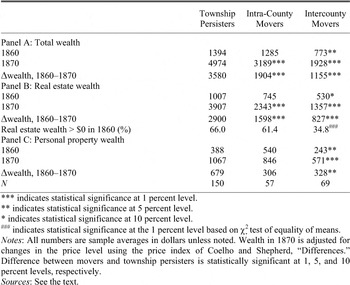
Panel A of Table 2 shows the accumulation of wealth in 1860 and 1870 of township persisters (N = 150), intra-county (short-distance) movers (N = 57), and intercounty (long-distance) movers (N = 69). Wealth in 1870 was adjusted for changes in the price level between
WEALTH ACCUMULATION OF PERSISTERS AND NON-PERSISTERS, 1860–1870

*** indicates statistical significance at 1 percent level.
** indicates statistical significance at 5 percent level.
* indicates statistical significance at 10 percent level.
### indicates statistical significance at the 1 percent level based on c2 test of equality of means.
Notes:
All numbers are sample averages in dollars unless noted. Wealth in 1870 is adjusted for changes in the price level using the price index of Coelho and Shepherd, “Differences.” Difference between movers and township persisters is statistically significant at 1, 5, and 10 percent levels, respectively.
Sources:
See the text.
1860 and 1870 using the regional price index of Philip R. P. Coelho and James F. Shepherd.Footnote 21 The most noticeable feature is the large gains in wealth of all households, regardless of their mobility status. Persisting and non-persisting households were substantially wealthier in 1870 than in 1860.
A comparison of the wealth of persisters and non-persisters shows, however, there appears to have been substantial returns to remaining in the same township over time. While persisters and movers to nearby townships had approximately equal amounts of initial wealth, persisters made much larger gains ($3,580 vs. $1,904) over the decade and were therefore substantially wealthier in 1870 than non-persisters ($4,974 vs. $3,189). Panel B shows the tendency of non-persisters to hold a smaller fraction of their wealth in 1860 in the form of real estate (72 percent vs. 58 percent), perhaps in anticipation of their moving, might explain some of this difference.
In comparison to township and county persisters, long-distance (intercounty) movers made more modest, but still large, absolute and percentage gains in wealth over the decade. The fraction of intercounty movers owning land in 1860 (Panel B) was much smaller than the corresponding fraction of county persisters, and accordingly, intercounty movers made much smaller gains in real estate wealth over the decade. Intercounty movers did, however, make absolute gains in personal property wealth approximately equal to those of intra-county movers (Panel C).
If the differences in wealth between persisters and non-persisters in Table 2 reflect the effects of persistence, the extent of geographic mobility on the frontier would be genuinely surprising. Given the high returns to staying in one place, migration should have been much less frequent. Assuming the effect is real, what might account for the difference in wealth accumulation between persisters and non-persisters? One source could have been the accumulation of location-specific knowledge about agriculture and markets. The other source was probably the heterogeneity of frontier land and the ability of the first settlers of an area to pick the best parcels.Footnote 22 Non-persisters may have had less choice about where to settle in their new locations. Competition for the best parcels might have been especially intense in areas undergoing rapid settlement.
A Regression Model of Geographic Persistence and Wealth Accumulation
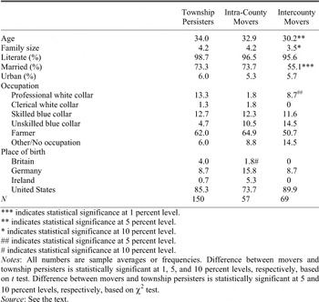
The differences in wealth between persisters and non-persisters in Table 2, however, may reflect not the effect of persistence on wealth but rather the omission of one or more explanatory variables. As Table 3 shows, there were significant differences between persisters and non-persisters in their observable characteristics such as age and occupation. For instance, the youth and blue-collar occupations of non-persisters could perhaps explain both their mobility and their lower wealth.
To control for differences between persisters and non-persisters in their observable characteristics, I estimate the effect of geographic persistence on wealth in 1870 in the following simple regression framework

THE 1860 CHARACTERISTICS OF PERSISTERS AND NON-PERSISTERS

*** indicates statistical significance at 1 percent level.
** indicates statistical significance at 5 percent level.
* indicates statistical significance at 10 percent level.
## indicates statistical significance at 5 percent level.
# indicates statistical significance at 10 percent level.
Notes:
All numbers are sample averages or frequencies. Difference between movers and township persisters is statistically significant at 1, 5, and 10 percent levels, respectively, based on t test. Difference between movers and township persisters is statistically significant at 5 and 10 percent levels, respectively, based on c2 test.
Source:
See the text.
where ln(wijk) is the natural logarithm of 1870 wealth for family i in county j in state (or territory) k, Xijk is a vector of observable characteristics (age, occupation, place of birth, family size, and literacy), and Zijk is a dummy variable equaling one if the family is observed in the same location (township or county) in 1860 and 1870 and equaling zero otherwise.Footnote 23 gk , lj , and mijk are, respectively, unobservable factors in the state (e.g., laws and institutions), in the county (e.g., local growing conditions and access to transportation), and specific to the individual (e.g., luck, talents, and motivation) affecting wealth. If persistence had a positive effect, q should have a positive sign.
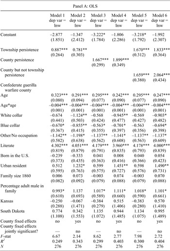
Table 4 reports results from the OLS estimation of equation 1. Panel A indicates a large and positive effect of geographic persistence on wealth. The coefficient on the persistence variable in column 1 implies that the wealth of township persisters in 1870 was 143 percent (e q − 1) higher than that of non-persisters, all else the same. The results also imply the following age-specific rate of wealth accumulation profile: 16.5 percent at age 20, 8.5 percent at age 30, and 0.5 percent at age 40. These rates are high and compare favorably to age-specific rates of wealth accumulation in other frontier areas.Footnote 24 When 1860 county fixed effects are included in equation 1 (column 2), the coefficient on persistence is slightly smaller but not statistically different than before, and the county fixed effects are jointly insignificant.Footnote 25
Columns 3 and 4 report the effect of persistence in a county. If township and county persisters accumulated wealth at approximately the same rates (i.e., migration to neighboring townships had a similar effect to remaining in the township), the effect of geographic persistence in columns 1 and 2 is biased downward. This appears to be the case. Column 3 indicates the effect of county persistence was to increase wealth by 429 percent. Again, inclusion of county fixed effects does not change the result, and the fixed effects are jointly insignificant (column 4). Columns 5 and 6 then show the results of a regression containing separate dummy variables for township persisters and intra-county movers. The coefficients in columns 5 and 6 are positive and statistically indistinguishable from each other and the coefficients in columns 3 and 4. Thus, township persisters and short-distance movers appear to have accumulated wealth at the same rate but at a rate higher than that of intercounty movers, all else the same.
An Instrumental Variables Analysis
The validity of the OLS results depends strongly on the assumption of the exogeneity of Z. Unfortunately, this assumption is unlikely to hold. On the frontier, unobservable factors affecting wealth accumulation likely also influenced persistence. For instance, a farmer's
THE EFFECT OF GEOGRAPHIC PERSISTENCE AND OTHER CHARACTERISTICS ON 1870 WEALTH


*** indicates statistical significance at 1 percent level.
** indicates statistical significance at 5 percent level.
* indicates statistical significance at 10 percent level.
Notes:
Omitted categories are farming for an occupation, born outside the United States, and residing in Nebraska in 1860.
business ties to local bankers and merchants might make him both more likely to persist and to accumulate wealth. The estimates of the effect of persistence on wealth would therefore be biased. Moreover, without knowing the nature of selection in persistence, it is not possible to say whether the coefficients are biased upward or downward.
To control for the simultaneity of geographic persistence and wealth, I reestimate equation 1 using instrumental variables (IV). Identification of q depends on finding a suitable instrument for Z, but the existence of such a variable in the census is not obvious. Instead, I use geographic variation in the incidence of armed raids and other small-scale guerilla warfare during the Civil War to generate exogenous migration.
The activities of Confederate guerillas in Kansas between 1862 and 1864 are well documented.Footnote 26 The raids were widespread and intended to sow fear in the pro-Union population of Kansas and to draw material and men away from the Union armies in the East. Most of the guerilla raids occurred in eastern Kansas, south of the Kaw (Kansas) River and north of Fort Scott.Footnote 27 A list of affected townships and counties is in the Appendix, but the most famous incident was the sacking of Lawrence in August 1863 by William Clarke Quantrill, which resulted in the deaths of 150 residents.Footnote 28
One result of the raids was thousands of refugees as Kansas residents fled their homes in mass. When the raids began, “[h]undreds of Kansans living along the border became panic-stricken and either moved back into the interior [of the state], abandoning crops and homes, or else left the state altogether,” wrote one historian.Footnote 29 By May 1863 newspapers reported that the border counties “from the Kaw [Kansas River] to Fort Scott” had been depopulated.Footnote 30
The flight of border residents potentially makes residence in a border county affected by this guerilla warfare a good instrument for persistence. Although the guerilla raids ended in 1864 and many refugees returned to their homes, a large number did not, electing to remain in their places of refuge permanently.Footnote 31 But because refugees fled their homes to escape violence and physical harm, their migration decisions were not guided primarily by economic considerations.
More generally, the validity of the instrumental variable hinges on the assumption that the raids influenced wealth only through their effect on persistence. This assumption could have been violated in a number of ways, however. One was the nonrandom selection of targets by Confederate guerillas. If the residents of targeted townships were more or less likely to accumulate wealth than nonresidents, the IV estimates of persistence's effect may be biased.
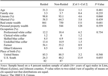
To investigate the nature of the raids, I constructed a 4 percent sample (N = 169) of the male, adult (older than 16 years of age) population of three border counties in Kansas (Johnson, Linn, and Lykins) from the 1860 U.S. Census. A comparison of residents of affected and unaffected townships shows only small and statistically insignificant differences in age, family size, marital status, real estate and personal property wealth, occupation, and country of birth (see Appendix Table 1). Thus, the raids appear to have been uncorrelated with wealth and most observable characteristics affecting wealth.Footnote 32
Another potential violation of the exogeneity of the instrumental variable was selective migration from raided counties. For instance, if those residents who were least able to accumulate wealth fled, then residency in a raided county would proxy for high ability and the IV estimates would be biased upward. However, migration from border counties appears to have been orthogonal to characteristics affecting wealth. First, when the persistence decision is regressed on the variables in X in equation 1 (i.e., the equivalent of the first stage of the IV model without the instrumental variable), none of the explanatory variables is statistically significant.Footnote 33 Adding 1860 real estate and personal property wealth as explanatory variables to proxy for unobserved ability yields the same result.Footnote 34 In contrast, when the first stage of the IV model is estimated using families in non-treated counties (N = 213), many of the explanatory variables, including age, wealth, and place of birth, are statistically significant. The causes of migration in raided counties thus appear random and fundamentally different from those in counties spared from the raids.
The sale of real estate or personal property by refugees before migration is still another potential source of endogeneity between the instrumental variable and wealth. The raids and the simultaneous flight of refugees may have created a glut in land and livestock markets that depressed prices and reduced the wealth of refugees. The terms of sale of refugees' property are unknown, but a number of factors suggest the effect of the raids on the wealth of refugees was minimal. First, most raids targeted towns and villages and left outlying areas untouched. The geographic scope of destruction was therefore limited. Another factor was that eastern Kansas had very fertile soils and received above average rainfall during the 1860s, resulting in high crop yields and land prices.Footnote 35 Last, the demands of the Union and Confederate armies for provisions kept the prices of crops and livestock and thus land values high.Footnote 36 All of these factors counteracted the depressing effects of the raids on property values and helped to preserve the wealth of refugees.
I estimate the IV model first using the subsample of Kansas families (because the Confederate raids occurred only in Kansas) and then the full sample of frontier families. Given their insignificance in the OLS model, county fixed effects are omitted from the models, though including them does not affect the results.Footnote 37
The second and fourth columns of Panel B of Table 4 show the first stage regression results. As expected, residence in a county afflicted by guerilla warfare had a negative and statistically significant effect on the likelihood of persistence. In the first model, residency was the only variable that affected migration in Kansas, decreasing the probability of persistence by 13 percentage points. In the second model, the effect of residency was −12 percentage points. For both IV models, I reject the hypothesis that the model is underidentified based on an Anderson canonical correlation test.Footnote 38
The first and third columns of Panel B of Table 4 show the second stage results. The effect of persistence on wealth in the first model (0.07) is much smaller than in the OLS models and close to zero. When the model is estimated using the whole sample of families (column 8), q is also significantly less than the OLS estimate and close to zero (0.247). Thus, when persistence and wealth are treated endogenously, the point estimates of q decrease substantially and are statistically insignificant. This suggests the large and positive OLS estimates in columns 1–6 are biased upward, reflecting either the negative selection of non-persisters or positive selection of persisters.Footnote 39
Although the IV analysis suggests persistence did not influence wealth, we should be cautious in drawing conclusions because q is estimated imprecisely. The large standard errors increase the probability of wrongly accepting the null hypothesis of no effect. The large standard errors may be the result of weakness in the relationship between the instrumental variable and persistence. The F-statistics from tests of the significance of the instrument in the first stages of the IV models are below the minimum of ten necessary to reject conclusively the hypothesis of weak instruments.Footnote 40 Thus, although the IV estimates of q have the desirable large sample property of consistency when persistence is endogenous, they are imprecisely estimated and thus leave some doubt about persistence's true effect.
The Sources of Wealth and Mobility on the Frontier
Consequently, while geographic persisters accumulated more wealth than non-persisters, it was not necessarily because of persistence. When the incidence of Confederate guerilla raids is used as an instrument for persistence, the effect of persistence on wealth drops significantly and is close to zero. This result appears robust to a number of potentially confounding factors including non-random guerilla raids and selective out-migration. The terms of sale of refugees' property are less certain, however. Note, though, that if refugees did sell their property at depressed prices, migration from raided counties would be associated with lower wealth in 1870 and the IV estimates of persistence's effect on wealth would be biased upward. This strengthens the conclusion that geographic persistence had a negligible effect on wealth.
The insignificance of persistence helps to explain the high rate of geographic mobility on the frontier. The cause of migration was most likely the opportunity to own land. The frontier was thinly populated, and thus land was cheap and plentiful. Non-persisters could therefore obtain farmland of comparable or superior quality to farmland in their places of origin. The subsequent population and economic development of newly settled areas then meant the real estate and the wealth of non-persisters appreciated rapidly.
A simple test of this hypothesis about the source of wealth of migrants is that wealth accumulation should have been correlated with the direction of migration. All else equal, opportunities for wealth accumulation should have been greater for families migrating west, because land was most plentiful in this direction. To test this hypothesis, the natural logarithm of 1870 wealth was regressed on a dummy variable for intercounty migration, an interaction variable between intercounty migration and a dummy variable indicating the direction of migration was west, and a set of control variables.Footnote 41 Because an instrumental variable for the direction of migration could not be found, the model was estimated by OLS.Footnote 42 The results (available upon request) show that conditional on migration, the direction of migration influenced wealth. The coefficient on the interaction variable for migration west is large, positive, and statistically significant (b = 0.958, s.e. = 0.512). This result supports the hypothesis about land having been a source of wealth of migrants. Opportunities for wealth accumulation seem to have been greater in less densely populated areas.Footnote 43
THE GEOGRAPHIC MOBILITY OF FRONTIER FAMILIES, 1870–1880

Notes:
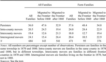
All numbers are percentages except number of observations. Persisters are families in the same township in 1870 and 1880. Intra-county movers are families in the same county in 1870 and 1880, but in different townships. Intercounty movers are families in different frontier counties in 1870 and 1880. Interregional movers are families living on the frontier in 1870, but not in 1880.
Sources:
See the text.
GEOGRAPHIC MOBILITY ON THE AGRICULTURAL FRONTIER, 1870–1880
While guerilla warfare in Kansas in the 1860s is useful for identifying migration's effect on wealth, patterns of migration during this period may have been unique. The 1870s were a more typical decade. The preceding section has suggested the opportunity to own land and to accumulate wealth was a cause of migration on the frontier. But who left? And where did non-persisters go?
The Destinations of Non-persisters, 1870–1880
Table 5 shows the distribution of frontier families by place of residence in 1870 and 1880. Persistence rates are shown separately for all families and for farm families and broken down further by length of residence on the frontier. Township persistence rates were low between 1870 and 1880. Just 36 percent of frontier inhabitants in 1870 could have been found in the same township a decade later. The rate of persistence was substantially higher (though still low in absolute terms) among families who had migrated to the frontier before 1860. Non-persisters were distributed approximately evenly across the other categories. Twenty percent of frontier families moved between townships in the same county. Another 20 percent moved between frontier counties. Almost a quarter of families left the region altogether.
In general, patterns of mobility of farm and non-farm families were similar. Farm families were slightly more likely to have persisted at the township or county level than nonfarm families. The township persist- ence rate of Kansas farmers was 39.5 percent, approximately equal to the rates Malin found in eastern and central Kansas over the same period.Footnote 44
The Characteristics of Persisters and Non-persisters, 1870–1880
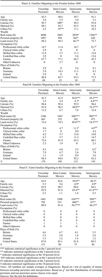
Did persisters and non-persisters differ systematically, and if so, how? Table 6 shows the mean 1870 characteristics of township persisters, intra-county movers, intercounty movers, and interregional movers. Because settlers with short tenure on the frontier seem to have been inherently more mobile than settlers with long tenure, Panels A and B of Table 6 disaggregate the means according to the time of migration (whether families migrated to the frontier before or after 1860). Panel C reports the mean characteristics of persisters and non-persisters who migrated to the frontier after 1860 and were farming in 1870.
Conditional on the time of migration to the frontier and occupation, there were few differences between township persisters and short- distance (intra-county) movers. The only statistically significant differences were with regard to literacy and urban residency. In contrast, there were significant differences between county persisters and non-persisters. In 1870 county persisters were several years older, had larger families, were wealthier, and were more likely to own land and to farm than non-persisters. In only a few respects, including place of birth, urban residency, and literacy, were the two groups alike.
A Regression Model of Geographic Mobility on the Frontier, 1870–1880
To explore the causes of geographic mobility more completely, I estimate an ordered probit model. In the model, families have four choices (denoted by z) about where to live. These choices vary according to their distance from the family's 1870 location.Footnote 45 From least to greatest distance, families could remain in their township of
THE 1870 CHARACTERISTICS OF GEOGRAPHIC PERSISTERS AND NON-PERSISTERS

*** indicates statistical significance at the 1 percent level.
** indicates statistical significance at the 5 percent level.
* indicates statistical significance at the 10 percent level.
### indicates statistical significance at the 1 percent level.
## indicates statistical significance at the 5 percent level.
# indicates statistical significance at the 10 percent level.
Notes:
All numbers are sample averages or frequencies. based on t test of equality of means between township persisters and non-persisters. Based on c2 test that distributions of township persisters and non-persisters across classes were equal.
Sources:
See the text for definitions.
residence in 1870 (z 1 = 1 if true, 0 otherwise), move to a different township in their county of residence in 1870 (z 2), move to a different county in Kansas, Nebraska, or the Dakota Territory (z 3), or move outside of the region (z 4). The opportunity to accumulate wealth would increase with distance moved (as a larger number of opportunities become available) but so would the probability of bad outcomes as ex-ante uncertainty increases. (It is assumed information about wages, land prices, growing conditions, etc. in prospective destinations becomes less precise with distance from the place of origin.) Three main factors probably determined distance moved: one's preferences for and ability to deal with risk, the ability to cope with “disequilibria” or a new physical, economic, and social environment, and the pecuniary, opportunity, and psychic costs of migration.Footnote 46 It is hypothesized that young, single, and educated (literate) persons would have been best able to deal with migration's risks and thus more willing to migrate long distances.
Let zijk* be the optimal distance from the 1870 location of family i in county j in state k and a linear function of observable characteristics (Wijk) and nk, wj, and eijk, which are, respectively, unobservable state, county, and individual characteristics affecting distance moved

Wijk includes 1870 variables for age, place of birth, literacy, wealth, occupation, family characteristics, and the time of migration to the frontier. The objective is to estimate λ, but z* is unobservable. Migration between townships, counties, and states is observable, however. Assume the location decision z is determined as follows:

where c 1, c 2, and c 3 are unknown thresholds determining the choice of where to live. If the error term has a normal distribution, the parameters of equation 2 and the unknown thresholds can be estimated in an ordered probit model.
Results
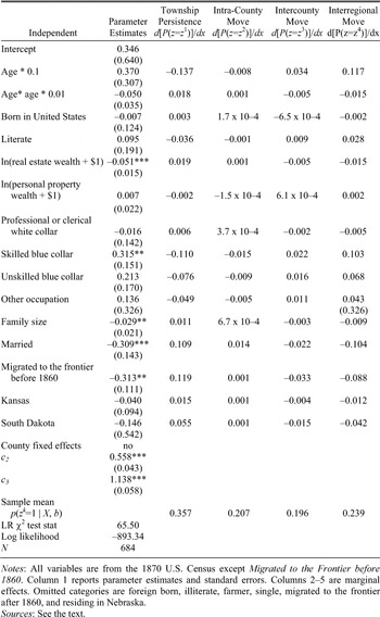
The ordered probit results are in Table 7 and show township persisters were more likely than non-persisters to have been old, married, farmers, and landowners.Footnote 47 The probability of persistence was quadratic in age and reached a minimum at 37 years. Marriage increased the likelihood of township persistence by 11 percentage
ORDERED PROBIT MODEL OF GEOGRAPHIC PERSISTENCE ON THE AGRICULTURAL FRONTIER, 1870–1880

Notes:
All variables are from the 1870 U.S. Census except Migrated to the frontier before 1860. Column 1 reports parameter estimates and standard errors. Columns 2–5 are marginal effects. Omitted categories are foreign born, illiterate, farmer, single, migrated to the frontier after 1860, and residing in Nebraska.
Sources:
see the text.
points, all else the same. Farmers (the omitted category) were 11 and 8 percentage points more likely to persist in townships than skilled and unskilled blue-collar workers. The probability of persistence was increasing in real estate wealth as well. Literacy had the expected positive effect on the probability of long-distance migration, but is not statistically significant. When the model is estimated with a set of county fixed effects, the results are essentially unchanged.Footnote 48
In general, the factors affecting migration on the frontier between 1870 and 1880 are consistent with the risks and benefits of migration increasing with distance moved. Young, blue-collar, and unattached persons had the most to gain and least to lose by moving long distances and thus could have coped best with migration's risks. For example, by moving to less densely populated areas where land was more plentiful, farm laborers might have become tenants or owners and increased their wealth. If migration proved less beneficial than expected, repeat migration could be undertaken at relatively small expense. In contrast, farm families would be giving up the security of their farms for the uncertain prospect of greater wealth. In addition, they had higher pecuniary and psychic costs of migration.
The factors affecting migration also help to explain patterns of wealth accumulation and mobility on the frontier. Young farm hands and other blue-collar workers were not just more likely to move, they were also less able to accumulate wealth than farm owners. These tendencies help to explain the high rate of geographic mobility and the superior wealth accumulation of persisters.
What Became of Frontier Non-persisters?
While long-distance migration was risky, little is actually known about the destinations of frontier non-persisters. Contrary to expectation, only a small percentage (20 percent) continued to migrate west and are observed in 1880 in the Mountain or Pacific census regions. Almost 60 percent relocated to the East North Central region (Wisconsin, Illinois, Indiana, Michigan, or Ohio (27.9 percent)) or to neighboring Minnesota, Iowa, or Missouri (the West North Central region (28.5 percent)). Thirteen percent could be found in the distant New England (5.5 percent) or Middle Atlantic (8.5 percent) regions. The remainder (9.7 percent) settled in the South. Thus, the popular perception of frontier non-persisters as incurable wanderers, ultimately destined for places and perhaps riches farther west, is inaccurate. Most migration from the frontier was return migration.Footnote 49
CONCLUSION
The frontier population was highly mobile. Only 39 percent of farmers in Kansas, Nebraska, and the Dakota Territory could be found in the same township in 1870 and 1880. Historians disagree about the meaning of mobility. One interpretation regards mobility as the result of economic hardship, while the other sees it as the result of widespread economic opportunity.
Based on an analysis of wealth and migration, this article concludes geographic mobility reflected the opportunity to accumulate wealth. Non-persisters fared as well as persisters in terms of wealth after controlling for the endogeneity of the migration decision. The source of the wealth of non-persisters was probably the opening of new lands for settlement along the leading edge of the frontier. Also, non-persisters tended to be young, single, landless, and blue collar and therefore to have the greatest net benefits of migration.
These findings are consistent with earlier research stressing the economic benefit of migration to the frontier.Footnote 50 Nonetheless, caution should be taken in extending this conclusion to other decades. The Civil War and immediate postwar eras were prosperous and perhaps exceptional. Other periods on the frontier may have been marked by more adverse circumstances and different patterns of mobility. For instance, Gary D. Libecap and Zeynep K. Hansen show during the late 1910s and early 1920s there were large numbers of farm failures, farm consolidations, and a decline in the rural population on the frontier because of prolonged drought.Footnote 51 This suggests that both hardship and economic opportunity were endemic to the frontier and the dangers of making generalizations about the sources of geographic mobility based on the study of one or two decades.
Appendix
The following describe the townships and counties experiencing Confederate guerilla raids between 1862 and 1864.Footnote 52
BOURBON COUNTY
Barnesville
Fort Lincoln
Fort Scott
Marmaton
Xenia
LINN COUNTY
Blooming Grove
Mine Creek
Mound City
Potosi
Trading Post
MIAMI (LYKINS) COUNTY
Osawatomie
Paola
JOHNSON COUNTY
Aubrey
Chilicothe
Gardner
Monticello
Olathe
Shawnee
Spring Hill
WYANDOTTE COUNTY
Wyandotte
CHARACTERISTICS OF RAIDED AND NON-RAIDED KANSAS TOWNSHIPS, 1860

Notes:
Sample based on a 4 percent random sample of adult (16+ years of age) males in Linn, Miami (Lykins), and Johnson counties. p-value refers to two-sided t test of equality of means or chi squared test that distributions are equal.
Source:
The 1860 U.S. Census.
LEAVENWORTH COUNTY
Leavenworth
DOUGLAS COUNTY
Baldwin City
Black Jack
Clinton
Lawrence
Lecompton
Marion
FRANKLIN COUNTY
Minneoloa
Pottawatomie
ALLEN COUNTY
Humboldt