1 Introduction
Mixing is a key process in many industrial applications and natural phenomena (Ottino Reference Ottino1989). Practical examples include glass manufacture, processing of food, microfluidic manipulations, and contaminant transport in the atmosphere, oceans and hydrological systems. During recent decades, substantial progress has been made in the description of mixing in systems as complex as turbulent flows (Kalda Reference Kalda2000; Shraiman & Siggia Reference Shraiman and Siggia2000; Warhaft Reference Warhaft2000; Falkovich, Gawedzki & Vergassola Reference Falkovich, Gawedzki and Vergassola2001; Duplat & Villermaux Reference Duplat and Villermaux2008), oceanic and atmospheric flows (Rhines & Young Reference Rhines and Young1983), the Earth’s mantle (Allègre & Turcotte Reference Allègre and Turcotte1986), porous media (Dentz et al. Reference Dentz, Leborgne, Englert and Bijeljic2011; Villermaux Reference Villermaux2012; Le Borgne, Dentz & Villermaux Reference Le Borgne, Dentz and Villermaux2015) and sheared particulate suspensions (Souzy et al. Reference Souzy, Lhuissier, Villermaux and Metzger2017). In particular, the conceptualization of scalar mixtures as ensembles of ‘lamellae’ evolving through stretching, diffusion and aggregation (Ranz Reference Ranz1979; Villermaux & Duplat Reference Villermaux and Duplat2003) has allowed the derivation of quantitative accurate theoretical predictions for the evolution of the full concentration probability density functions (PDFs) for a broad range of flows. Within this framework (valid for lamellae thinner than the smallest scale within the flow), mixing is driven by three processes occurring simultaneously: (i) stretching a scalar field by a given flow, creating elongated lamellar structures, (ii) diffusion and compression, which compete to define concentration gradients, and (iii) lamella coalescence leading ultimately to the final homogeneity of the system (Duplat & Villermaux Reference Duplat and Villermaux2008).
In complex configurations such as those listed above, the evolution of the concentration distribution is sensitive to a number of characteristics of the system: the distribution of stretching rates, the macroscopic dispersion rate, the scalar molecular diffusion coefficient and the rate at which lamellae aggregate. While their influence on the dynamics of mixing is clear from a theoretical point of view, they can rarely be observed independently. Moreover, in spite of the numerous experimental studies on mixing, the question of the spatial resolution required to quantify the evolution of a concentration field has received little attention. This latter point is obviously crucial, since under-resolved images, by artificially broadening the concentration distribution of isolated lamellae, or conversely, by sharpening the concentration distribution of bundles of adjacent lamellae, lead to an erroneous appreciation of the mixing rate.
Here, we present highly resolved experiments where the basic mechanisms governing mixing are quantified individually: the formation of elongated lamellae by stretching, the establishment of a Batchelor scale by competition between compression and diffusion, the enhancement of diffusive mixing by stretching, and the diffusive aggregation of lamellae. We consider for this a lamella formed by photobleaching of a fluorescent dye in a laminar shear flow where the concentration distribution can be quantified using a well-controlled experimental set-up, built specifically to resolve small length scales. This benchmark experiment was chosen precisely because it is well established theoretically. Unambiguous conclusions can therefore be drawn regarding the spatial resolution required to capture the evolution of the concentration distribution of an isolated lamella, and more generally within any mixing protocols. Moreover, it illustrates, with an unprecedented resolution and level of detail, the basic lamellar theories for mixing at the scale of a single lamella. Last, we investigate the coalescence of two nearby lamellae, specifically focusing on its impact on the evolution of the concentration distribution. The theoretical prerequisites are recalled in § 2. After presenting the experimental set-up in § 3, the measurements are reported in § 4. Conclusions are drawn in § 5.
2 Mixing in a laminar shear flow
2.1 General picture
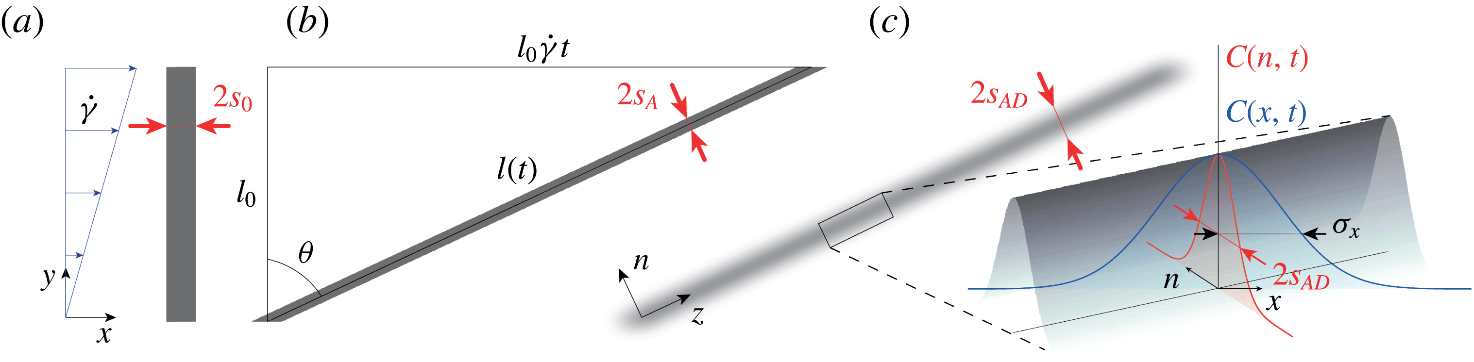
We consider a lamella of dye of length
 $l_{0}$
and half-width
 $s_{0}$
initially positioned perpendicular to the flow, as illustrated in figure 1(a). As the lamella is advected by a laminar shear flow with a shear rate
 $\dot{\unicode[STIX]{x1D6FE}}$
, its length increases as
 $l(t)=l_{0}\sqrt{1+(\dot{\unicode[STIX]{x1D6FE}}t)^{2}}$
. Thus, considering the sole effect of the advection field (for now neglecting that of molecular diffusion), the half-width of the lamella
 $s_{A}(t)$
decreases following
 $s_{A}(t)=s_{0}/\sqrt{1+(\dot{\unicode[STIX]{x1D6FE}}t)^{2}}$
(see figure 1
b) since in this two-dimensional flow, mass conservation prescribes
 $s_{0}l_{0}=s_{A}(t)l(t)$
. The effect of the shear flow can thus be quantified by a compression rate
 $(-1/s_{A})(\text{d}s_{A}/\text{d}t)$
which describes how fast the lamella transverse dimension thins down owing to its stretching by the advection field. Conversely, molecular diffusion tends to broaden the lamella with a diffusive broadening rate
 $D_{0}/s_{A}^{2}$
, where
 $D_{0}$
is the molecular diffusion coefficient of the scalar. Balancing these two rates,
 $(-1/s_{A})(\text{d}s_{A}/\text{d}t)\sim D_{0}/s_{A}^{2}$
and assuming
 $\dot{\unicode[STIX]{x1D6FE}}t\gg 1$
, naturally defines a time scale, also called the Batchelor time,
 $t_{B}\sim Pe^{1/3}/\dot{\unicode[STIX]{x1D6FE}}$
, where
 $Pe=\dot{\unicode[STIX]{x1D6FE}}s_{0}^{2}/D_{0}$
denotes the Péclet number. This time corresponds to the onset of the homogenization of the concentration levels within the system, beyond which the concentration levels within the lamella start to decay significantly.
(a) Schematic of a lamella of dye of initial length
 $l_{0}$
and half-width
 $s_{0}$
advected in a laminar shear flow. (b) Effect of the advection field alone: the strain
 $\dot{\unicode[STIX]{x1D6FE}}t$
has stretched the lamella and thinned down its transverse dimension to
 $2s_{A}(t)$
. (c) Effect of both advection and molecular diffusion: at the same strain, the half-width of the lamella is denoted
 $s_{AD}(t)$
. Inset: schematic of the Gaussian concentration field of the lamella with its concentration profiles along the flow
 $C(x,t)$
and transverse to the lamella
 $C(n,t)$
.

2.2 Exact solution
The complete description of the evolution of the lamella of dye can be found by directly solving the full advection–diffusion equation
 $$\begin{eqnarray}\frac{\unicode[STIX]{x2202}C}{\unicode[STIX]{x2202}t}+\boldsymbol{u}\boldsymbol{\cdot }\unicode[STIX]{x1D735}C=D_{0}\unicode[STIX]{x1D6FB}^{2}C,\end{eqnarray}$$
where
 $\boldsymbol{u}=(\dot{\unicode[STIX]{x1D6FE}}y,0,0)$
denotes the advection field, and
 $C$
the concentration field.
This equation can be simplified (Ranz Reference Ranz1979; Rhines & Young Reference Rhines and Young1983; Ottino Reference Ottino1989; Meunier & Villermaux Reference Meunier and Villermaux2003, Reference Meunier and Villermaux2010) if written in a moving frame
 $(n,z)$
aligned with the directions of maximal compression and stretching of the lamellae (see figure 1
c), and by using Ranz’s transform (Ranz Reference Ranz1979), which uses warped time units,
 $\unicode[STIX]{x1D70F}=\int _{0}^{t}D_{0}/s_{A}^{2}(t^{\prime })\,\text{d}t^{\prime }$
, and distances normalized by the lamella transverse dimension,
 $\unicode[STIX]{x1D709}=n/s_{A}(t)$
. Equation (2.1) then reduces to a simple diffusion equation
 $$\begin{eqnarray}\frac{\unicode[STIX]{x2202}C}{\unicode[STIX]{x2202}\unicode[STIX]{x1D70F}}=\frac{\unicode[STIX]{x2202}^{2}C}{\unicode[STIX]{x2202}\unicode[STIX]{x1D709}^{2}},\end{eqnarray}$$
whose solution for an initial Gaussian concentration profile with maximum
 $C_{0}$
is
 $$\begin{eqnarray}C(\unicode[STIX]{x1D709},\unicode[STIX]{x1D70F})=\frac{C_{0}}{\sqrt{1+4\unicode[STIX]{x1D70F}}}\text{e}^{-(\unicode[STIX]{x1D709}^{2}/(1+4\unicode[STIX]{x1D70F}))}.\end{eqnarray}$$
The maximum concentration of the lamella thus decays with time according to
 $$\begin{eqnarray}C_{max}(t)=\frac{C_{0}}{\sqrt{1+4\unicode[STIX]{x1D70F}}}.\end{eqnarray}$$
Since the half-width of the lamella in Ranz’s units is
 $\unicode[STIX]{x1D70E}_{\unicode[STIX]{x1D709}}=(1+4\unicode[STIX]{x1D70F})^{1/2}$
(see (2.3)), the transverse dimension of the lamella
 $s_{AD}(t)$
, accounting both for the effect of advection and diffusion, and expressed in standard unit of length, is
 $$\begin{eqnarray}s_{AD}(t)=\unicode[STIX]{x1D70E}_{\unicode[STIX]{x1D709}}s_{A}(t)=\frac{s_{0}(1+4\unicode[STIX]{x1D70F})^{1/2}}{\sqrt{1+(\dot{\unicode[STIX]{x1D6FE}}t)^{2}}}.\end{eqnarray}$$
The latter expression gives access to the half-width of the lamella along the flow (
 $x$
-direction)
 $$\begin{eqnarray}\unicode[STIX]{x1D70E}_{x}(t)=\frac{s_{AD}(t)}{\cos \unicode[STIX]{x1D703}}=\unicode[STIX]{x1D70E}_{0}(1+4\unicode[STIX]{x1D70F})^{1/2},\end{eqnarray}$$
with
 $\unicode[STIX]{x1D70E}_{0}=s_{0}$
and
 $\cos \unicode[STIX]{x1D703}=1/\sqrt{1+(\dot{\unicode[STIX]{x1D6FE}}t)^{2}}$
(see figure 1).
We now have access to a more accurate estimation of the Batchelor time, which by definition is reached when
 $\unicode[STIX]{x1D70F}=1$
(Ranz Reference Ranz1979). Since
 $\unicode[STIX]{x1D70F}=D_{0}(t+\dot{\unicode[STIX]{x1D6FE}}^{2}t^{3}/3)/s_{0}^{2}$
, the Batchelor time, for
 $Pe\gg 1$
, is
 $$\begin{eqnarray}t_{B}\approx \frac{(3Pe)^{1/3}}{\dot{\unicode[STIX]{x1D6FE}}}.\end{eqnarray}$$
At this time, the transverse dimension of the lamella, from now on referred to as the Batchelor scale (Batchelor Reference Batchelor1959), is found to be
 $$\begin{eqnarray}s_{AD}(t_{B})=s_{0}\sqrt{5}(3Pe)^{-1/3}.\end{eqnarray}$$
Last, the evolution of the concentration distribution
 $P(C,t)$
of the lamella can be derived. Using the following change of variables
 $P(C)\,\text{d}C=P(x)\,\text{d}x$
yields
 $P(C)=P(x)|\text{d}C/\text{d}x|^{-1}$
, which can easily be expressed from
 $$\begin{eqnarray}C(x,t)=C_{max}(t)\text{e}^{-x^{2}/\unicode[STIX]{x1D70E}_{0}^{2}(1+4\unicode[STIX]{x1D70F})},\end{eqnarray}$$
and the uniformity of
 $P(x)$
. Considering the range of concentration
 $C_{th}\leqslant C\leqslant C_{max}(t)$
, above any arbitrary threshold concentration
 $C_{th}$
(larger than the experimental background noise), one obtains
 $$\begin{eqnarray}P(C,t)=\frac{1}{\unicode[STIX]{x1D6FD}C\sqrt{\ln (C_{max}/C)}},\end{eqnarray}$$
where
 $\unicode[STIX]{x1D6FD}$
is a normalizing prefactor ensuring that
 $\int _{C_{th}}^{C_{max}(t)}P(C,t)\,\text{d}C=1$
.
The above set of equations fully describes the evolution of a lamella of dye advected in a laminar shear flow.
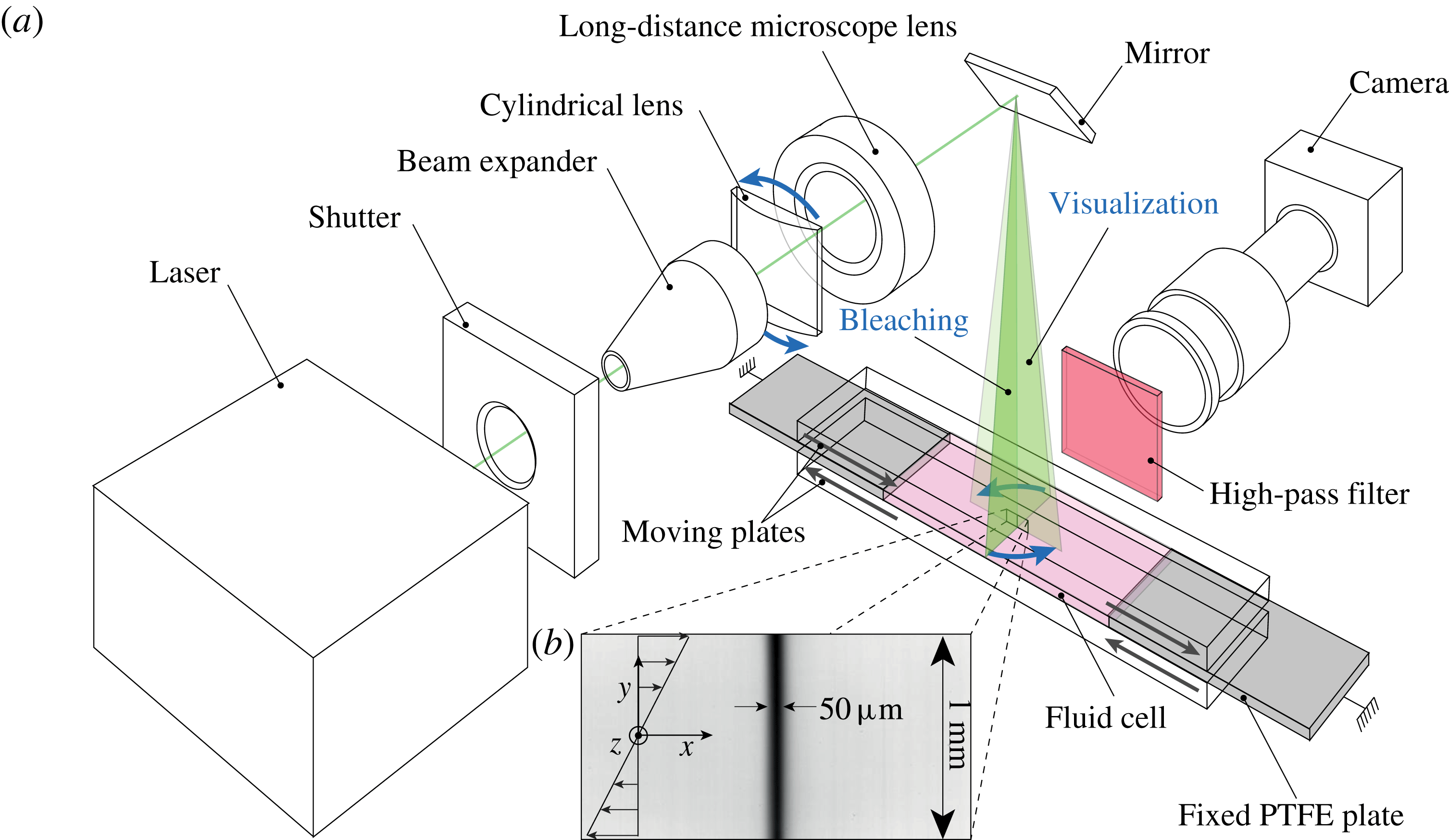
(a) Schematic of the set-up. (b) Typical image of a lamella obtained by photobleaching.

3 Experimental set-up
The experimental set-up is shown in figure 2. It consists of a shear cell made of two parallel Plexiglas plates sandwiching a fluid cell 85 mm long, 25 mm wide and of height
 $h=3~\text{mm}$
. The fluid is sheared by setting the two plates into opposite motion with two high-resolution translation stages (not shown on the schematic). The travel range of the plate enables a maximum strain of 30. The cell is sealed on both ends by two PTFE plates (grey in figure 2), and on the sides by two transparent sidewalls (not shown on the schematic) mounted on the bottom moving plate.
The fluid is a Newtonian mixture of Triton X-100 (77.4 wt. %), zinc chloride (13.4 wt. %) and water (9.2 wt. %) having a density
 $\unicode[STIX]{x1D70C}=1.19~\text{g}~\text{cm}^{-3}$
and viscosity
 $\unicode[STIX]{x1D702}=4.2~\text{Pa}~\text{s}$
, which ensures laminar flow conditions (over the full range of shear rates investigated the Reynolds number is
 $Re=\unicode[STIX]{x1D70C}\dot{\unicode[STIX]{x1D6FE}}h^{2}/\unicode[STIX]{x1D702}\leqslant 10^{-3}$
). Prior to filling the cell, some fluorescent dye (Rhodamine 6G) is thoroughly mixed to the fluid at a concentration of
 $2\,\,10^{-6}~\text{g}~\text{ml}^{-1}$
. The molecular diffusion coefficient of this dye was measured in the cell with the fluid at rest using a technique similar to that reported in Souzy et al. (Reference Souzy, Lhuissier, Villermaux and Metzger2017). We find
 $D_{0}\approx 2.66\,\,10^{-13}~\text{m}^{2}~\text{s}^{-1}$
at a temperature of
 $22~^{\circ }\text{C}$
.
The initial lamella is generated using photobleaching, (Axelrod et al.
Reference Axelrod, Koppel, Schlessinger, Elson and Webb1976). A high-power laser-diode beam (Laser Quantum Gem512-2.5W) is shaped into a thin laser sheet using the combination of lenses set in their ‘bleaching’ configuration, as shown in figure 2(a). This sheet, oriented in the
 $y-z$
plane (perpendicular to the flow) and used with full intensity, locally changes the conformation of the rhodamine molecules, which irreversibly become unable to fluoresce.
Then, the set-up is set into its ‘visualization’ configuration by rotating the cylindrical lens
 $90^{\circ }$
: this orients the laser sheet along the
 $x-y$
plane (along the flow). The lamella then appears as a thin dark vertical line (see figure 2
b). Note that the initial lamella is in fact a transverse sheet, rather than just a line. This avoids diffusion in the
 $z$
-direction and enables us to study a purely two-dimensional process. This photobleaching technique, relative to a direct injection of fluorescent dye, also ensures well-controlled initial conditions: the lamella is uniform and its initial concentration profile is Gaussian owing to the Gaussian nature of the impacting laser beam.
Immediately after bleaching, the fluid is sheared at the desired shear rate and images of the evolution of the lamella are acquired using a camera (Basler Ace2000-50 gm,
 $2048\times 1080~\text{pixel}^{2}$
, 12 bit) coupled to a high-resolution macroscope (Leica Z16
 $\text{APO}\times 1$
). The set-up was designed to provide an image resolution (
 $0.8~\unicode[STIX]{x03BC}\text{m}~\text{pixel}^{-1}$
) small enough to resolve the Batchelor scale (2.8). For instance, with
 $\dot{\unicode[STIX]{x1D6FE}}=0.01~\text{s}^{-1}$
and
 $s_{0}=25~\unicode[STIX]{x03BC}\text{m}$
, we have
 $s_{AD}(t_{B})=s_{0}\sqrt{5}(3\dot{\unicode[STIX]{x1D6FE}}s_{0}^{2}/D_{0})^{-1/3}\approx 10~\unicode[STIX]{x03BC}\text{m}$
. A high-pass filter (590
 $\,$
nm) is positioned between the sample and the camera to eliminate direct light reflections. To avoid photobleaching during the image acquisition, the intensity of the laser is lowered to 100 mW and the image acquisition is synchronized with a shutter opening only during acquisition times. Note that all experiments are performed at
 $T=22\pm 0.05~^{\circ }\text{C}$
by setting the temperature of the water running through the bottom moving plate with a cryo-thermostat.
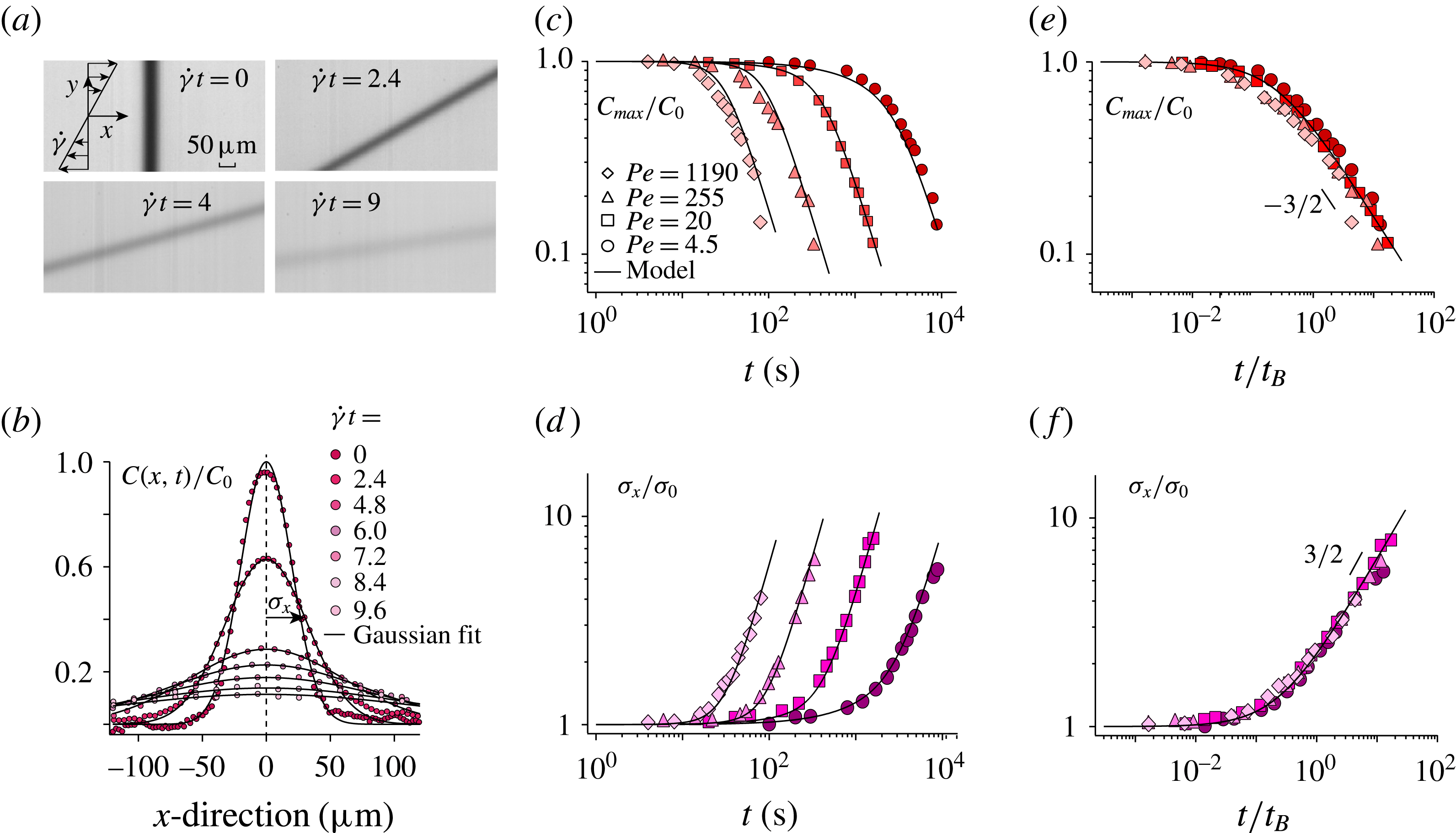
(a) Successive images of a lamella undergoing shear at
 $Pe=20$
(see also supplementary movie 1 available at https://doi.org/10.1017/jfm.2017.916). (b) Corresponding averaged concentration profiles along the flow (
 $x$
-direction). The black lines are fitting Gaussian profiles. (c) Normalized maximum concentration
 $C_{max}/C_{0}$
and (d) normalized half-width of the concentration profiles
 $\unicode[STIX]{x1D70E}_{x}/\unicode[STIX]{x1D70E}_{0}$
versus time for experiments performed at different Péclet numbers. The black lines correspond to (2.4) in (c) and (2.6) in (d). In both cases,
 $\dot{\unicode[STIX]{x1D6FE}}$
,
 $s_{0}$
and
 $D_{0}$
are set and fixed by the experimental conditions. (e) and (f) Same data plotted versus
 $t/t_{B}$
.

4 Experimental results
4.1 A single lamella
Figure 3(a) shows successive pictures of a lamella undergoing a laminar shear (see also supplementary movie 1). Initially vertical and highly contrasted, the lamella progressively tilts under the effect of the shear flow while blurring under the effect of molecular diffusion. Accurate measurement of the lamella’s concentration profile along the flow (
 $x$
-direction) are obtained by averaging over all horizontal lines of pixels after translating these lines to make their maximum concentration coincide. The resulting average concentration profile of the lamella is shown in figure 3(b) for successive strains: the maximum concentration decays while the width increases. These trends are captured well by fitting each concentration profile with a Gaussian of the form
 $C(x,t)=C_{max}(t)\text{e}^{-x^{2}/\unicode[STIX]{x1D70E}_{x}^{2}(t)}$
(see figure 3
b).
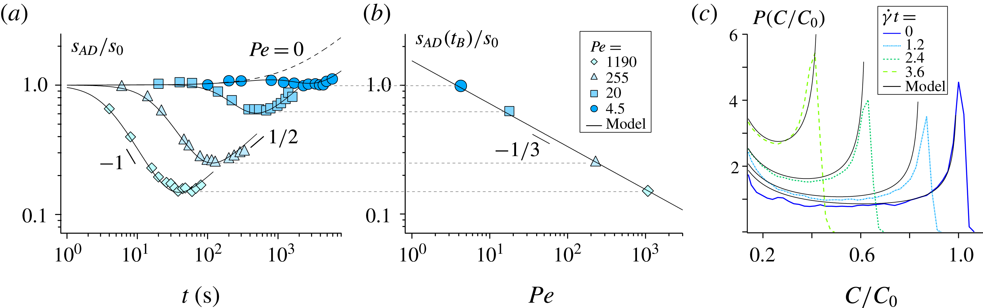
(a) Evolution of transverse dimension of the lamella
 $s_{AD}(t)/s_{0}$
versus time for experiments performed at different Péclet numbers. The black lines correspond to (2.5). The dotted line corresponds to the solution in the absence of shear, i.e. in the pure diffusion limit (
 $Pe=0$
). (b) Corresponding Batchelor scale
 $s_{AD}(t_{B})/s_{0}$
versus Péclet number; the black line corresponds to (2.8). (c) Concentration distribution
 $P(C/C_{0})$
measured at successive strains,
 $\dot{\unicode[STIX]{x1D6FE}}t$
, for a lamella sheared at
 $Pe=4.5$
. The black lines correspond to (2.10). In all cases,
 $\dot{\unicode[STIX]{x1D6FE}}$
,
 $s_{0}$
and
 $D_{0}$
are fixed by the experimental conditions.

The resulting maximum concentration
 $C_{max}(t)$
and width
 $\unicode[STIX]{x1D70E}_{x}(t)$
are plotted in figures 3(c) and 3(d) versus time for experiments performed at different Péclet number (
 $4.5\leqslant Pe\leqslant 1190$
). The Péclet number was varied by repeating the experiment at various shear rates
 $\dot{\unicode[STIX]{x1D6FE}}=[6\times 10^{-4}-0.3]~\text{s}^{-1}$
. The agreement with (2.4) and (2.6) is very good for both
 $C_{max}(t)$
and
 $\unicode[STIX]{x1D70E}_{x}(t)$
. Note that in both cases,
 $\dot{\unicode[STIX]{x1D6FE}}$
,
 $s_{0}$
and
 $D_{0}$
are fixed by the experimental conditions; there is thus no adjustable parameter. When plotted as a function of the dimensionless time
 $t/t_{B}$
, where
 $t_{B}=(3Pe)^{1/3}/\dot{\unicode[STIX]{x1D6FE}}$
is the Batchelor time, these data are found to collapse, for all
 $Pe$
, on the same master curve (see figure 3
e,f). For
 $t<t_{B}$
,
 $C_{max}$
and
 $\unicode[STIX]{x1D70E}_{x}$
remain constant. Then when the effect of molecular diffusion becomes significant, i.e for
 $t>t_{B}$
,
 $C_{max}$
(respectively
 $\unicode[STIX]{x1D70E}_{x}$
) starts to decrease (respectively increase) following the power law
 $t^{-3/2}$
(respectively
 $t^{3/2}$
), consistently with the long-time trends of (2.4) and (2.6). These measurements clearly illustrate how mixing is accelerated by imposing an external macroscopic shear: larger applied shear rates (larger Péclet numbers) result in earlier mixing times.
We have so far probed the lamella along the direction of the flow. However, further insight into the mixing process, specifically on the advection–diffusion coupling presented above, are provided by probing the lamella width along its transverse direction (along
 $n$
, see figure 1). Figure 4(a) shows the evolution of
 $s_{AD}(t)$
measured experimentally. At an intermediate time, the thickness of the lamella is found to decrease like
 $t^{-1}$
. After reaching a minimum, it increases like
 $t^{1/2}$
. These trends precisely illustrate the expected interplay between advection and diffusion. The lamella width initially decreases as imposed by the kinematics of the flow following the intermediate time trend (for
 $t<t_{B}$
) of (2.5),
 $s_{AD}(t)\sim s_{0}(\dot{\unicode[STIX]{x1D6FE}}t)^{-1}$
. However, this compression of the lamella progressively steepens its concentration gradients which, beyond the Batchelor time, eventually makes the broadening effect due to molecular diffusion become dominant. The transverse dimension of the lamella then re-increases diffusively like
 $t^{1/2}$
. At the Batchelor time
 $t_{B}$
, the lamella typically reaches its minimum thickness, which is equal to the Batchelor scale
 $s_{AD}(t_{B})$
(within 3 %). As shown in figure 4(b), reporting this direct measurement of the Batchelor scale obtained for various Péclet numbers matches the expected prediction
 $s_{AD}(t_{B})=s_{0}\sqrt{5}(3Pe)^{-1/3}$
(see (2.8)).
To fully describe the mixing process, we also measure the evolution of the lamella’s concentration distribution
 $P(C,t)$
. The distribution
 $P(C)$
is obtained from the histogram of intensities collected from all the pixels constituting the lamella which are above a threshold
 $C_{th}=0.1C_{0}$
. This discards the background image noise, enabling us to focus on the peak of interest, that of high concentration. Changing the value of the threshold above the background noise changes the extent of the spatial domain over which
 $P(C)$
is computed, but it does not affect its shape. We obtain concentration distributions which have a characteristic U-shape (Ottino Reference Ottino1989) (see figure 4
c). The distribution’s maximum probability, initially located at
 $C=C_{0}$
, progressively drifts to lower values as the lamella is stretched and diffuses. The prediction provided by (2.10) is in good agreement with the measured concentration distributions obtained for all Péclet numbers and, again, without adjustable parameter.
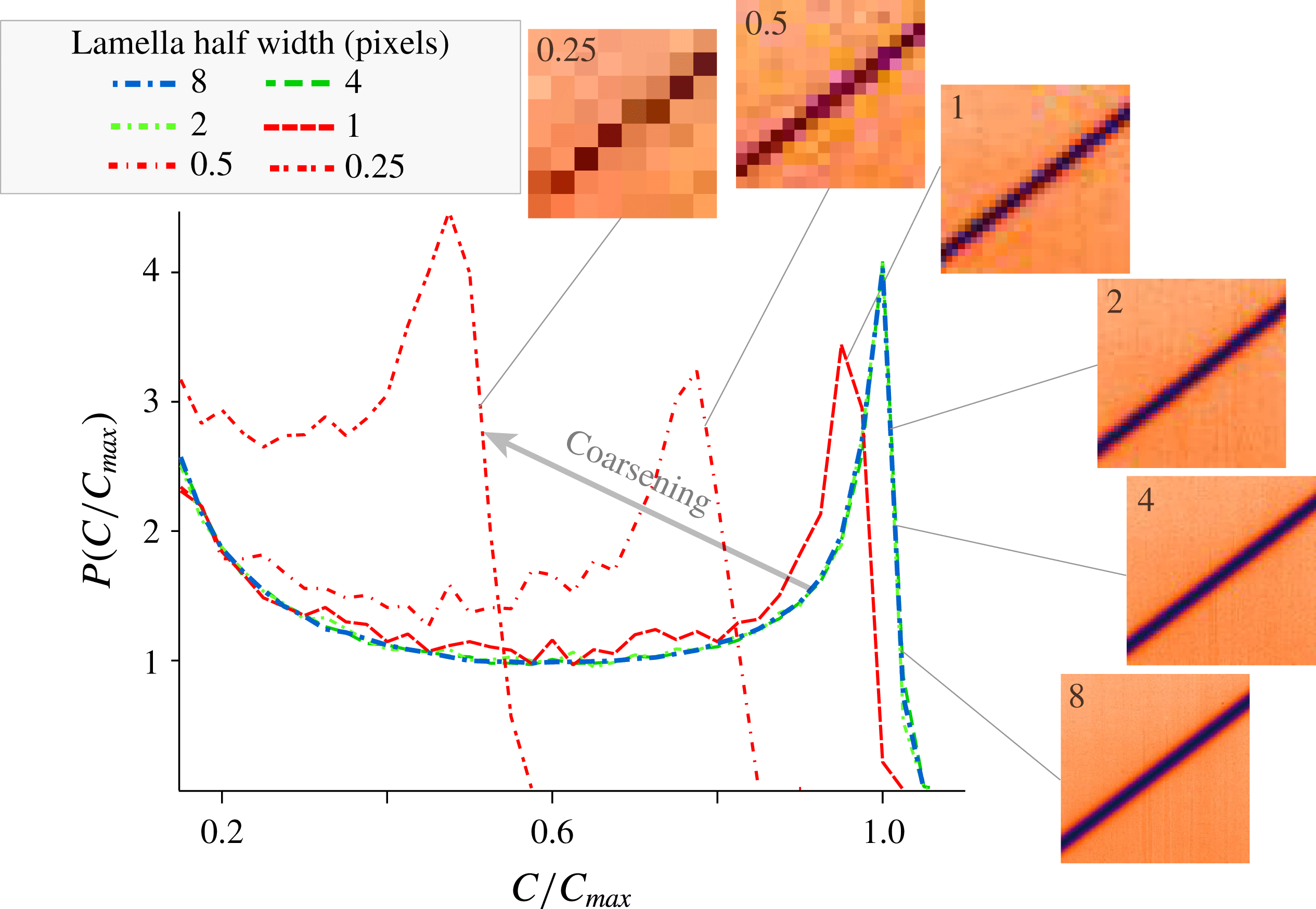
Distributions of concentration
 $P(C/C_{max})$
obtained from the progressive digital coarsening of an experimental image.

The distributions shown above are well resolved since the Batchelor scale is always larger than 10 pixels. However, in most studies on mixing, such a high resolution is not achieved. Moreover, when mixing is investigated in complex systems such as turbulent flows (Duplat & Villermaux Reference Villermaux and Duplat2006), porous media (Le Borgne et al. Reference Le Borgne, Dentz and Villermaux2015), or recently in sheared particulate suspensions (Souzy et al. Reference Souzy, Lhuissier, Villermaux and Metzger2017), the initial lamella of dye does not evolve towards a single lamella with uniform thickness but, instead, towards a large number of lamellae having widely distributed thicknesses. In such situations, it is important to know which part of the distribution of lamellae can be resolved experimentally.
To address this point, we systematically investigate how the set-up spatial resolution can bias the measured concentration distribution of a single lamella. This can be achieved by a simple coarsening protocol: the reference concentration distribution (blue dotted line in figure 5) is obtained from a highly resolved image where the lamella half-width spans
 $8$
pixels. When coarsening the pixels of this reference image, (merging
 $2\times 2$
pixels into one,
 $4\times 4$
pixels into one and so on) we find that the concentration distribution remains unchanged for images having
 $4$
and
 $2$
pixels across the lamella half-width (green dotted lines in figure 5). Conversely, larger coarsening, i.e. images having
 $1$
pixel or less across the lamella half-width, yield erroneous results: the concentration distribution departs from the reference one (red dotted lines in figure 5). The limit of
 $1$
pixel per lamella half-width is surprisingly small and comes as encouraging news for experimentalists. This limit holds as long as the concentration profile is smooth (e.g Gaussian) and there is a finite tilt between the lamella and the lines of pixels. In such case, the progressive drift of the lamella position relative to that of the pixels scans all the possible concentration levels, thereby providing results consistent with the fully resolved PDF.
4.2 Two lamellae
As mentioned in the introduction, mixing in complex systems generally involves coalescence between dispersed lamellae. This latter step is crucial for the system to reach its final homogeneity. Here, the photobleaching technique is used to produce two adjacent lamellae and investigate a single coalescence event.
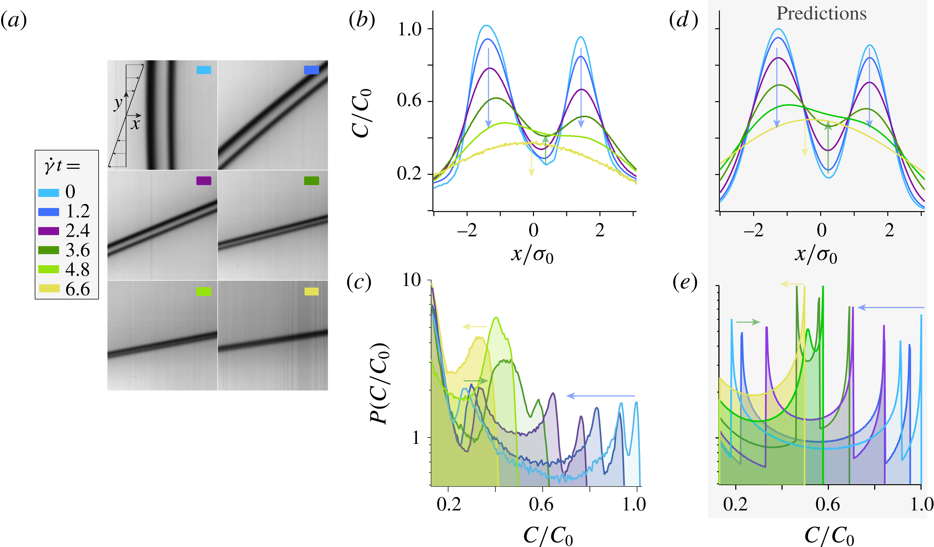
(a) Coalescence of two nearby lamellae advected in a laminar shear flow (see also supplementary movie 2). Evolution of the corresponding experimental (b) concentration profiles and (c) concentration distributions obtained at successive strains
 $\dot{\unicode[STIX]{x1D6FE}}t$
. Predictions for the evolution of (d) the concentration profiles and (e) the concentration distributions at the same strains. Again,
 $\dot{\unicode[STIX]{x1D6FE}}$
,
 $s_{0}$
and
 $D_{0}$
are fixed by the experimental conditions.

Figure 6(a) shows images of two parallel lamellae captured at successive strains (see also supplementary movie 2). The two lamellae are initially distinct from each other and, as they are stretched by the flow and diffuse, they progressively merge to eventually form one single entity. The evolution of their concentration profiles measured along the flow
 $x$
-direction are shown in figure 6(b). The two maxima of concentration, corresponding to each lamella, decay (blue arrows) while the minimum located in between increases (green arrow). This goes on until the two lamellae merge into one single lamella whose maximum subsequently decreases (yellow arrow). This evolution can easily be predicted owing to the linearity of the diffusion equation: the concentration profile of a set of two lamellae, with individual profiles
 $C_{1}(x,t)$
and
 $C_{2}(x,t)$
, is simply obtained from the summation
 $C(x,t)=C_{1}(x,t)+C_{2}(x,t)$
(Fourier Reference Fourier1822). Using, for each lamella, equation (2.9) with the initial experimental maximum intensity and width, we thereby obtain the concentration profiles shown in figure 6(d).
To anticipate the impact of this coalescence on the evolution of the concentration distribution, let us recall that
 $P(C)\sim |\text{d}C/\text{d}x|^{-1}$
. Thus, each value of
 $C(x,t)$
where the concentration profile presents an horizontal slope gives rise to a peak in the concentration distribution. This can be clearly observed on the experimental concentration distributions shown in figure 6(c). As long as the two lamellae are distinct, one not only observes two peaks at high concentration (corresponding to the maximum of concentration of each lamellae), but also one peak at low concentration (corresponding to the minimum concentration located in between the two lamellae). Then, as the lamellae are stretched and diffuse, the two peaks corresponding to the two concentration maxima move to the left (blue arrow in figure 6
c). Conversely, as the concentration in between the two lamellae increases, the low concentration peak moves to the right (green arrow in figure 6
c). Coalescence occurs when the three peaks collide; the distribution eventually recovers its characteristic U-shape as the lamellae have coalesced into a single entity. The same phenomenology can be observed on the concentration distributions obtained from numerically computing the slope of the predicted concentration profiles (see figure 6
e).
5 Discussion and conclusions
We have explored experimentally the basic mechanisms of mixing in stirred flows by thoroughly investigating the evolution of an initially segregated scalar (a lamella of fluorescent dye) stretched within a laminar shear flow. A high-resolution set-up, using a photobleaching technique to generate and control the shape of the initial lamella, was built in order to resolve length scales at which diffusion plays a significant role. Our measurements of the evolution of the lamella concentration profiles and concentration distributions are, without adjustable parameter, in excellent quantitative agreement, for
 $Pe=[4.5-1190]$
, with the theoretical predictions.
We also investigated the evolution of the lamella’s transverse dimension, which conspicuously illustrates the advection–diffusion coupling yielding at intermediate time to a
 $t^{-1}$
compression of the lamella dominated by the kinematics of the flow, followed, after the Batchelor time, by a
 $t^{1/2}$
broadening dominated by molecular diffusion. The Batchelor scale, which to our knowledge has been observed experimentally only once (Meunier et al.
Reference Meunier, Huck, Nobili and Villermaux2015), was here measured systematically for various Péclet numbers and found to follow the expected behaviour,
 $s_{AD}(t_{B})/s_{0}=\sqrt{5}(3Pe)^{-1/3}$
.
Most importantly, through a coarsening protocol, we determined the minimal experimental spatial resolution required to resolve the concentration distribution of a single lamella: its half-width must be larger than 1 pixel. This requirement is general and constrains the measurement of any mixing protocol. Indeed, for all stretching protocols, lamellae reach their minimum thickness at the Batchelor time while they are still isolated individual entities. Resolving
 $P(C)$
at this time, which requires one to resolve each individual lamella, therefore is the most demanding in term of spatial resolution: the half-width of the lamella at the Batchelor time,
 $s_{AD}(t_{B})$
, shall at least span 1 pixel. Note that measuring
 $P(C)$
at longer times can be less stringent. Indeed, beyond the Batchelor time, lamellae diffuse sufficiently that, when their spacing becomes sufficiently small, nearby lamellae start merging together. The concentration gradients then no longer vary over the lamellae transverse dimension but, instead, over a larger length scale which reflects the size of the bundles of merging lamellae. In the context of turbulent mixtures for instance, this ‘coarse-grained scale’ was proposed to follow
 $\unicode[STIX]{x1D702}=LSc^{-2/5}$
, where
 $L$
denotes the stirring length and
 $Sc$
the Schmidt number (Duplat & Villermaux Reference Villermaux and Duplat2006). However, the latter length scale is only relevant after lamellae have merged, which occurs after the Batchelor time. Therefore, resolving
 $P(C)$
at all times requires an experimental spatial resolution satisfying
 $s_{AD}(t_{B})>1$
pixel.
Finally, we have investigated the coalescence between two lamellae and its impact on the evolution of the concentration distribution. Lamellae’s overlap gives rise to a non-trivial peak at low concentration. This observation is important as it may be relevant to interpret more complex situations.
To conclude, the high-resolution experimental techniques developed for the present study, and the determination of their limitations, open promising perspectives for future studies on mixing.
Acknowledgements
We thank E. Villermaux and P. Meunier for their inspiring comments and suggestions. We would also like to thank S. Noel for machining the experimental set-up. This work was supported by ANR JCJC SIMI 9, by the Labex MEC ANR-10-LABX-0092, by ANR-11-IDEX-0001-02 and by ERC consolidator grant ReactiveFronts 648377.
Supplementary movies
Supplementary movies are available at https://doi.org/10.1017/jfm.2017.916.