Turbulent mixing due to the Holmboe wave instability at high Reynolds number

Hesam Salehipour; C. P. Caulfield; W. R. Peltier

doi:10.1017/jfm.2016.488

Turbulent mixing due to the Holmboe wave instability at high Reynolds number

Published online by Cambridge University Press: 30 August 2016

Hesam Salehipour

C. P. Caulfield and

W. R. Peltier

Show author details

Hesam Salehipour*: Affiliation:
Department of Physics, University of Toronto, Toronto, ON M5S 1A7, Canada
C. P. Caulfield: Affiliation:
BP Institute, University of Cambridge, Madingley Road, Cambridge CB3 0EZ, UKDepartment of Applied Mathematics and Theoretical Physics, University of Cambridge, Centre for Mathematical Sciences, Wilberforce Road, Cambridge CB3 0WA, UK
W. R. Peltier: Affiliation:
Department of Physics, University of Toronto, Toronto, ON M5S 1A7, Canada
*: †Email address for correspondence: h.salehipour@utoronto.ca

Article contents

Abstract
Introduction
Computational and analysis strategy
Results
Conclusions
References

Rights & Permissions

Abstract

We consider numerically the transition to turbulence and associated mixing in stratified shear flows with initial velocity distribution $\overline{U}(z,0)\,\boldsymbol{e}_{x}=U_{0}\,\boldsymbol{e}_{x}\tanh (z/d)$ and initial density distribution $\overline{\unicode[STIX]{x1D70C}}(z,0)=\unicode[STIX]{x1D70C}_{0}[1-\tanh (z/\unicode[STIX]{x1D6FF})]$ away from a hydrostatic reference state $\unicode[STIX]{x1D70C}_{r}\gg \unicode[STIX]{x1D70C}_{0}$ . When the ratio $R=d/\unicode[STIX]{x1D6FF}$ of the characteristic length scales over which the velocity and density vary is equal to one, this flow is primarily susceptible to the classic well-known Kelvin–Helmholtz instability (KHI). This instability, which typically manifests at finite amplitude as an array of elliptical vortices, strongly ‘overturns’ the density interface of strong initial gradient, which nevertheless is the location of minimum initial gradient Richardson number $Ri_{g}(0)=Ri_{b}=g\unicode[STIX]{x1D70C}_{0}d/\unicode[STIX]{x1D70C}_{r}U_{0}^{2}$ , where $Ri_{g}(z)=-([g/\unicode[STIX]{x1D70C}_{r}]\,\text{d}\overline{\unicode[STIX]{x1D70C}}/\text{d}z)/(\text{d}\overline{U}/\text{d}z)^{2}$ and $Ri_{b}$ is a bulk Richardson number. As is well known, at sufficiently high Reynolds numbers ( $Re$ ), the primary KHI induces a vigorous but inherently transient burst of turbulence and associated irreversible mixing localised in the vicinity of the density interface, leading to a relatively well-mixed region bounded by stronger density gradients above and below. We explore the qualitatively different behaviour that arises when $R\gg 1$ , and so the density interface is sharp, with $Ri_{g}(z)$ now being maximum at the density interface $Ri_{g}(0)=RRi_{b}$ . This flow is primarily susceptible to Holmboe wave instability (HWI) (Holmboe, Geophys. Publ., vol. 24, 1962, pp. 67–113), which manifests at finite amplitude in this symmetric flow as counter-propagating trains of elliptical vortices above and below the density interface, thus perturbing the interface so as to exhibit characteristically cusped interfacial waves which thereby ‘scour’ the density interface. Unlike previous lower- $Re$ experimental and numerical studies, when $Re$ is sufficiently high the primary HWI becomes increasingly more three-dimensional due to the emergence of shear-aligned secondary convective instabilities. As $Re$ increases, (i) the growth rate of secondary instabilities appears to saturate and (ii) the perturbation kinetic energy exhibits a $k^{-5/3}$ spectrum for sufficiently large length scales that are influenced by anisotropic buoyancy effects. Therefore, at sufficiently high $Re$ , vigorous turbulence is triggered that also significantly ‘scours’ the primary density interface, leading to substantial irreversible mixing and vertical transport of mass above and below the (robust) primary density interface. Furthermore, HWI produces a markedly more long-lived turbulence event compared to KHI at a similarly high $Re$ . Despite their vastly different mechanics (i.e. ‘overturning’ versus ‘scouring’) and localisation, the mixing induced by KHI and HWI is comparable in both absolute terms and relative efficiency. Our results establish that, provided the flow Reynolds number is sufficiently high, shear layers with sharp density interfaces and associated locally high values of the gradient Richardson number may still be sites of substantial and efficient irreversible mixing.

JFM classification

Turbulent Flows: Stratified turbulence Waves/Free-surface Flows: Wave breaking

Information

Type: Papers
Information: Journal of Fluid Mechanics , Volume 803 , 25 September 2016, pp. 591 - 621
DOI: https://doi.org/10.1017/jfm.2016.488 [Opens in a new window]
Copyright: © 2016 Cambridge University Press

1 Introduction

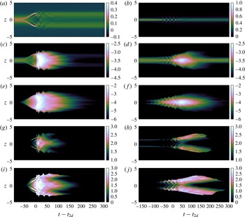
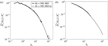
Stably stratified parallel shear flows, in which both the background velocity and density distribution vary with height, are very common in the natural environment, and understanding how they become turbulent and irreversibly mix the density field is of central importance to modelling the fate and transport of momentum, heat and chemical species. There exists a substantial body of research into the dynamics of such flows (see e.g. the reviews of Peltier & Caulfield (Reference Peltier and Caulfield2003) and Ivey, Winters & Koseff (Reference Ivey, Winters and Koseff2008)), with much of it focusing on the mixing triggered by the breakdown to turbulence of primary shear instabilities of the initial laminar flow.

A commonly considered model problem is the hyperbolic tangent stratified shear layer, where the base velocity and density distributions are represented in dimensional form as

(1.1)

$$\begin{eqnarray}\displaystyle & \displaystyle \overline{U}(z,0)\,\boldsymbol{e}_{x}=U_{0}\tanh \left(\frac{z}{d}\right)\boldsymbol{e}_{x}, & \displaystyle\end{eqnarray}$$

(1.2)

$$\begin{eqnarray}\displaystyle & \displaystyle \overline{\unicode[STIX]{x1D70C}}(z,0)=\unicode[STIX]{x1D70C}_{0}\left[1-\tanh \left(\frac{z}{\unicode[STIX]{x1D6FF}}\right)\right], & \displaystyle\end{eqnarray}$$

where

$U_{0}=\unicode[STIX]{x0394}U/2$ and

$\unicode[STIX]{x1D70C}_{0}=\unicode[STIX]{x0394}\unicode[STIX]{x1D70C}/2$ , respectively, denote half the velocity and density jump across the interface and

$\boldsymbol{e}_{x}$ is the unit vector in the streamwise

$x$ -direction. Note that the density field employed in this paper represents departures from a hydrostatic state that is associated with a constant reference density

$\unicode[STIX]{x1D70C}_{r}$ . In addition,

$\unicode[STIX]{x1D70C}_{r}\gg \unicode[STIX]{x1D70C}_{0}$ such that the Boussinesq approximation is valid. The linear stability of this flow is characterised by a bulk Richardson number

$Ri_{b}$ , the thickness ratio of shear to density interfaces

$R$ , the Reynolds number

$Re$ and the Prandtl number

$Pr$ , defined as

(1.3a-d )

$$\begin{eqnarray}\displaystyle Ri_{b}=\frac{g\unicode[STIX]{x1D70C}_{0}d}{\unicode[STIX]{x1D70C}_{r}U_{0}^{2}},\quad R=\frac{d}{\unicode[STIX]{x1D6FF}},\quad Re=\frac{U_{0}d}{\unicode[STIX]{x1D708}},\quad Pr=\frac{\unicode[STIX]{x1D708}}{\unicode[STIX]{x1D705}}, & & \displaystyle\end{eqnarray}$$

where $g$ is the acceleration due to gravity, $\unicode[STIX]{x1D708}$ is the kinematic viscosity and $\unicode[STIX]{x1D705}$ is the molecular diffusivity of the density field.

When the ratio $R=d/\unicode[STIX]{x1D6FF}=1$ , the gradient Richardson number, $Ri_{g}(z)$ , increases monotonically from its minimum value $Ri_{g}(0)=Ri_{b}$ at the midpoint of the stratified shear layer. For sufficiently small values of $Ri_{b}$ , and large enough values of $Re$ , this flow is susceptible to the classic Kelvin–Helmholtz instability (KHI), an inviscid instability whose growth rate is decreased monotonically by ambient stratification. This instability manifests itself at finite amplitude as an array of elliptical vortices or billows which ‘roll up’ or ‘overturn’ the primary density interface. Although the KHI has long been considered a key mechanism by which turbulence is triggered and through which irreversible mixing occurs in stratified flows, it has only recently been appreciated that both the character of the transition and ensuing mixing are profoundly modified for $Re\gtrsim 4000$ (defined as in (1.3)) (Mashayek & Peltier Reference Mashayek and Peltier2013; Mashayek, Caulfield & Peltier Reference Mashayek, Caulfield and Peltier2013) and when the Prandtl number $Pr$ is increased from $O(1)$ characteristic of gases to $O(10)$ characteristic of liquids such as water (Salehipour, Peltier & Mashayek Reference Salehipour, Peltier and Mashayek2015).

Indeed, for fluids with $Pr\neq 1$ , as argued in Smyth, Klaassen & Peltier (Reference Smyth, Klaassen and Peltier1988), it is perhaps more natural to consider the stability of flows with length scale ratio $R=\sqrt{Pr}$ . For such flows, with a ‘sharp’ density interface embedded within a broader shear layer, the stability properties are qualitatively different, as $Ri_{g}(z)$ now is maximum at the midpoint of the shear layer $Ri_{g}(0)=RRi_{b}$ for sufficiently large values of $R$ , and drops to small values as $|z|$ increases (Smyth & Winters Reference Smyth and Winters2003; Alexakis Reference Alexakis2005). Therefore, for sufficiently large values of $Ri_{b}$ , the flow becomes unstable to an inherently stratified instability, which we shall refer to as the Holmboe wave instability (HWI), originally identified by Holmboe (Reference Holmboe1962). At finite amplitude, the (symmetric) HWI develops into propagating elliptical vortical patches above and below the density interface, which induce characteristically cusped waves on the density interface itself.

Current understanding of the nonlinear behaviour of this instability is based on previous relatively low- $Re$ experimental (Strang & Fernando Reference Strang and Fernando2001; Zhu & Lawrence Reference Zhu and Lawrence2001; Hogg & Ivey Reference Hogg and Ivey2003; Tedford, Pieters & Lawrence Reference Tedford, Pieters and Lawrence2009; Carpenter et al. Reference Carpenter, Tedford, Rahmani and Lawrence2010; Meyer & Linden Reference Meyer and Linden2014) and numerical studies (Smyth et al. Reference Smyth, Klaassen and Peltier1988; Smyth & Peltier Reference Smyth and Peltier1989, Reference Smyth and Peltier1991; Smyth & Winters Reference Smyth and Winters2003; Smyth Reference Smyth2006; Smyth, Carpenter & Lawrence Reference Smyth, Carpenter and Lawrence2007; Carpenter, Lawrence & Smyth Reference Carpenter, Lawrence and Smyth2007; Carpenter et al. Reference Carpenter, Tedford, Rahmani and Lawrence2010) in which the induced flow is essentially dominated by molecular effects and thus the associated turbulent mixing is minimal (i.e. the total effective diffusion of density is of the order of the molecular diffusivity). Based on their direct numerical simulation (DNS) of HWI at $Re=300$ (when defined consistently with (1.3)), Smyth & Winters (Reference Smyth and Winters2003) and Smyth et al. (Reference Smyth, Carpenter and Lawrence2007) have shown that HWI may ‘never become turbulent’ under strongly stratified conditions and furthermore its overall cumulative mixing may be dominated by its long-lived quasi-linear preturbulent stage. Therefore the turbulent mixing due to HWI has been commonly observed to be relatively weak, with the vertical irreversible transport of mass being restricted to the ejection of thin wisps of fluid from the tips of the cusped waves (see e.g. Carpenter et al. Reference Carpenter, Tedford, Rahmani and Lawrence2010). To our knowledge, there is no evidence in the literature for the onset of recognisable and geophysically relevant turbulent motions produced by HWI, to the extent that it is unclear whether energetic turbulence may be triggered by this instability at all.

However, this uncertainty essentially arises from consideration of flows with relatively small Reynolds number $Re\sim O(100)$ due to experimental and computational challenges in considering sufficiently large and fast flows with still ‘sharp’ density gradients. Since the turbulent mixing properties of the KHI are now known to change so substantially for $Re\gtrsim 4000$ and $Pr\sim O(10)$ , it seems a natural question to investigate whether such a ‘mixing transition’ (using the terminology of Dimotakis (Reference Dimotakis2005)) also occurs for flows susceptible to primary HWI, and so in this paper we describe the first series of analyses based on DNS of a flow susceptible to a primary HWI with relatively high $Re$ ( $Re=4000$ and $6000$ ) and compare the results of these simulations with similar results from simulations at much lower $Re$ values. Specifically, we aim to understand the effects of increasing $Re$ on (i) the transition to a turbulent phase of HWI, (ii) the stratified turbulence that is engendered and (iii) the induced irreversible mixing. Furthermore, at sufficiently high $Re$ , we aim to compare the mixing properties of HWI with an appropriately equivalent flow susceptible to KHI, in particular to establish whether it is possible for substantial instantaneous turbulent mixing still to occur when a sharp density interface, embedded within a shear flow, is not ‘overturned’ by strong vortices centred on it, but rather ‘scoured’ by vortices on either side (Woods et al. Reference Woods, Caulfield, Landel and Kuesters2010).

To achieve these objectives, the rest of the paper is organised as follows. In § 2 we briefly review our computational and analysis strategy, which includes discussions of the energetics and spectral analysis in § 2.1, mixing analysis in § 2.2 and the relevant length scales in § 2.3. We present our quantitative results in § 3, demonstrating in § 3.1 the effects of increasing $Re$ on the evolution of HWI, its spectra and its induced mixing. Moreover, we demonstrate in § 3.2 that, at sufficiently high $Re$ , turbulent breakdown mediated by primary HWI leads to substantial irreversible mixing, comparable in magnitude and efficiency to that induced by primary KHI, yet qualitatively different in its spatiotemporal distribution. Finally, we offer conclusions based upon these results in § 4.

2 Computational and analysis strategy

We consider flows with initial velocity and density distributions given in (1.1) and (1.2), and non-dimensionalise the governing incompressible Boussinesq equations using $\unicode[STIX]{x1D70C}_{0}$ , $U_{0}$ and $d$ to obtain

(2.1)

$$\begin{eqnarray}\displaystyle & \displaystyle \unicode[STIX]{x1D735}\boldsymbol{\cdot }\boldsymbol{u}=0, & \displaystyle\end{eqnarray}$$

(2.2)

$$\begin{eqnarray}\displaystyle & \displaystyle \frac{\unicode[STIX]{x2202}\boldsymbol{u}}{\unicode[STIX]{x2202}t}+\boldsymbol{u}\boldsymbol{\cdot }\unicode[STIX]{x1D735}\boldsymbol{u}=-\unicode[STIX]{x1D735}p-Ri_{b}\unicode[STIX]{x1D70C}\boldsymbol{e}_{z}+\frac{1}{Re}\unicode[STIX]{x1D6FB}^{2}\boldsymbol{u}, & \displaystyle\end{eqnarray}$$

(2.3)

$$\begin{eqnarray}\displaystyle & \displaystyle \frac{\unicode[STIX]{x2202}\unicode[STIX]{x1D70C}}{\unicode[STIX]{x2202}t}+\boldsymbol{u}\boldsymbol{\cdot }\unicode[STIX]{x1D735}\unicode[STIX]{x1D70C}=\frac{1}{Re\,Pr}\unicode[STIX]{x1D6FB}^{2}\unicode[STIX]{x1D70C}, & \displaystyle\end{eqnarray}$$

in which

$p$ denotes the deviation of the pressure field from hydrostatic balance. The above equations also reveal the significance of the three parameters

$Re$ ,

$Pr$ and

$Ri_{b}$ as defined in (1.3). The non-dimensional forms of the reduced gravity

$g^{\prime }=(\unicode[STIX]{x1D70C}_{0}/\unicode[STIX]{x1D70C}_{r})g$ , the kinematic viscosity

$\unicode[STIX]{x1D708}$ and the thermal diffusivity

$\unicode[STIX]{x1D705}$ can thus be related straightforwardly to these parameters as

$g^{\prime }=Ri_{b}=Ri_{g}(0)/R$ ,

$\unicode[STIX]{x1D708}=Re^{-1}$ and

$\unicode[STIX]{x1D705}=Re^{-1}Pr^{-1}$ .

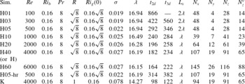
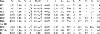
As tabulated in table 1, we consider nine simulations with $Pr=8$ and $Ri_{b}=0.16$ . For simulation ‘K’ at $Re=4000$ , we set $R=1$ and so $Ri_{g}(0)=0.16$ with the flow being susceptible to a primary KHI. For the other simulations, designated by ‘Hxx’, where the digits ‘xx’ indicate $Re\times 10^{-2}$ , we set $R=Pr^{1/2}=\sqrt{8}$ (Smyth et al. Reference Smyth, Klaassen and Peltier1988) and so $Ri_{g}(0)\simeq 0.45$ , with the flow being susceptible to a primary HWI. For most of these simulations, we set the streamwise extent to be one wavelength $\unicode[STIX]{x1D706}$ of the linear mode with the largest real growth rate $\unicode[STIX]{x1D70E}$ obtained by solving the full viscously diffusive Taylor–Goldstein equation. In order to allow Holmboe waves to merge (i.e. to investigate whether or not the pairing instability emerges), we set the streamwise extent of simulations ‘H01’, ‘H03’ and ‘H05’ to be $L_{x}=2\unicode[STIX]{x1D706}$ (see table 1 for further details). Note that, for the purpose of the discussion to follow, we have repeated simulation ‘H05’ (designated ‘H05-hr’) at a higher resolution, similar to that of ‘H40’.

We employ the spectral element code Nek5000 (Fischer Reference Fischer1997) to conduct our DNS analyses. The reader is referred to Salehipour & Peltier (Reference Salehipour and Peltier2015) and Salehipour et al. (Reference Salehipour, Peltier and Mashayek2015) (and the references therein) for details of the numerical methodology and resolution requirements (see also the Appendix for a note on resolution). The boundary conditions are assumed to be periodic in the horizontal directions while the top and bottom boundaries are assumed to be free-slip, impermeable for velocity and insulating for the density field. The simulations are initialised with the initial base flow distributions given in (1.1) and (1.2), which are perturbed by adding both a two-dimensional fluctuation in the form of the eigenfunction of the appropriate linear instability mode and three-dimensional white noise to the velocity field to excite secondary instabilities in an unbiased manner. The amplitudes of both these added fluctuations, namely $5\times 10^{-2}$ for two-dimensional and $5\times 10^{-3}$ for three-dimensional perturbations, when scaled with $U_{0}$ , are small enough to ensure a posteriori that the associated volume-averaged perturbation kinetic energy is at least six orders of magnitude smaller than the volume-averaged mean flow kinetic energy.

Table 1.

Details of the three-dimensional DNS in which the total grid points are approximately $p^{3}N_{x}N_{y}N_{z}$ , where $p=10$ is the order of Lagrange polynomial interpolants and $N_{x}$ , $N_{y}$ and $N_{z}$ denote the number of spectral elements within the horizontal ( $L_{x}$ ), spanwise ( $L_{y}$ ) and vertical ( $L_{z}$ ) extents of the computational domain; $N_{z}^{c}$ represents the number of elements within a central region of the domain with height $L_{z}^{c}=10$ . Outside of $L_{z}^{c}$ , the adjacent elements of the grid are gradually stretched by a factor of 1.25 %. In all these simulations, $L_{y}=3$ and $L_{z}=30$ . Also, $\unicode[STIX]{x1D70E}$ is the real part of the growth rate of the primary instability with a wavelength $\unicode[STIX]{x1D706}$ . The times $t_{2d}$ and $t_{3d}$ are, respectively, the characteristic time of maximum amplitude of the spanwise-averaged perturbation and the characteristic time of the maximum amplitude of the inherently three-dimensional deviation from this perturbation (as defined in the text).

2.1 Energetics and spectral analysis

The total velocity field, $\boldsymbol{u}(x,y,z,t)$ , can be decomposed into a mean (denoted by an overbar) and a perturbation component defined as

(2.4)

$$\begin{eqnarray}\displaystyle & \displaystyle \boldsymbol{u}(x,y,z,t)=\overline{U}(z,t)+\boldsymbol{u}^{\prime }(x,y,z,t), & \displaystyle\end{eqnarray}$$

(2.5)

$$\begin{eqnarray}\displaystyle & \displaystyle \overline{U}(z,t)=\langle \boldsymbol{u}\rangle _{xy}, & \displaystyle\end{eqnarray}$$

in which

$\langle ~\rangle _{h}$ denotes averaging in the

$h$ -direction. For example,

$\langle ~\rangle _{xy}$ indicates horizontal averaging or

$\langle ~\rangle _{xyz}$ indicates volume averaging. For convenience, we also denote horizontal averaging with an overbar.

The perturbation velocity field may in turn be subdivided into spanwise-averaged two-dimensional perturbations and inherently three-dimensional perturbations, defined as (Caulfield & Peltier Reference Caulfield and Peltier2000)

(2.6)

$$\begin{eqnarray}\displaystyle & \displaystyle \boldsymbol{u}^{\prime }(x,y,z,t)=[u_{2d}+u_{3d},v_{3d},w_{2d}+w_{3d}], & \displaystyle\end{eqnarray}$$

(2.7)

$$\begin{eqnarray}\displaystyle & \displaystyle (u_{2d},0,w_{2d})(x,z,t)=\langle (u-\overline{U},v,w)\rangle _{y}, & \displaystyle\end{eqnarray}$$

(2.8)

$$\begin{eqnarray}\displaystyle & \displaystyle (u_{3d},v_{3d},w_{3d})(x,y,z,t)=(u-\overline{U}-u_{2d},v,w-w_{2d}). & \displaystyle\end{eqnarray}$$

Following this triple Reynolds decomposition, the total kinetic energy includes contributions from three individual reservoirs (Caulfield & Peltier Reference Caulfield and Peltier2000). These reservoirs are (i) the horizontally averaged kinetic energy $\overline{\mathscr{K}}$ associated with the background stratified shear layer which is evolving in time, (ii) the two-dimensional spanwise-averaged kinetic energy $\mathscr{K}_{2d}$ associated with the two-dimensional perturbations away from the background mean flow and (iii) the inherently three-dimensional kinetic energy $\mathscr{K}_{3d}$ . In addition, the potential energy budget can also be subdivided into two components (Winters et al. Reference Winters, Lombard, Riley and D’Asaro1995; Caulfield & Peltier Reference Caulfield and Peltier2000), consisting of (i) the potential energy that is associated with a notional statically stable reference state, $\mathscr{P}_{B}$ , or equivalently the background potential energy (BPE) and (ii) the amount of potential energy that is available to be converted back into either the kinetic energy or BPE, which is known as the available potential energy (APE) or $\mathscr{P}_{A}$ (Lorenz Reference Lorenz1955). Thus we can write

(2.9)

$$\begin{eqnarray}\displaystyle & \displaystyle \mathscr{K}=\overline{\mathscr{K}}+\mathscr{K}^{\prime }=\overline{\mathscr{K}}+\mathscr{K}_{2d}+\mathscr{K}_{3d}, & \displaystyle\end{eqnarray}$$

(2.10)

$$\begin{eqnarray}\displaystyle & \displaystyle \mathscr{P}=\mathscr{P}_{A}+\mathscr{P}_{B}, & \displaystyle\end{eqnarray}$$

in which each individual reservoir of kinetic energy takes the common volume-averaged form

$\widetilde{\mathscr{K}}=0.5\langle \tilde{\boldsymbol{u}}\boldsymbol{\cdot }\tilde{\boldsymbol{u}}\rangle _{xyz}$ , where

$\tilde{\boldsymbol{u}}$ is replaced by the respective velocity vector (e.g.

$\tilde{\boldsymbol{u}}=(u_{3d},v_{3d},w_{3d})$ for

$\mathscr{K}_{3d}$ ). Furthermore, BPE or

$\mathscr{P}_{B}$ is obtained through a continuous adiabatic rearrangement of the instantaneous density field into a statically stable profile,

$\unicode[STIX]{x1D70C}_{\ast }(z)$ , at each step in the process of flow evolution (Winters et al. 1995; Caulfield & Peltier 2000). Salehipour et al. (2015) presented a parallel implementation of the ‘sorting’ procedure required to find

$\unicode[STIX]{x1D70C}_{\ast }(z)$ . Therefore, the potential energy reservoirs in (2.10) are defined as

(2.11a-c )

$$\begin{eqnarray}\displaystyle \mathscr{P}=Ri_{b}\langle \unicode[STIX]{x1D70C}z\rangle _{xyz},\quad \mathscr{P}_{B}=Ri_{b}\langle \unicode[STIX]{x1D70C}_{\ast }z\rangle _{z},\quad \mathscr{P}_{A}=\mathscr{P}-\mathscr{P}_{B}. & & \displaystyle\end{eqnarray}$$

The horizontal two-dimensional Fourier transform (denoted by a hat) of the perturbation velocity field $\boldsymbol{u}^{\prime }(x,y,z,t)$ is defined as

(2.12)

$$\begin{eqnarray}\displaystyle \widehat{\boldsymbol{u}^{\prime }}(k_{x},k_{y},z,t)=\iint \boldsymbol{u}^{\prime }(x,y,z,t)\text{e}^{-\text{i}(k_{x}x+k_{y}y)}\,\text{d}x\,\text{d}y, & & \displaystyle\end{eqnarray}$$

in which $k_{x}$ and $k_{y}$ represent the streamwise and spanwise wavenumbers, respectively.

We now define the spectral decomposition of the perturbation kinetic energy associated with the streamwise ( $\widehat{\mathscr{K}_{x}^{\prime }}$ ), spanwise ( $\widehat{\mathscr{K}_{y}^{\prime }}$ ) and vertical ( $\widehat{\mathscr{K}_{z}^{\prime }}$ ) components of the perturbation velocity field as

(2.13)

$$\begin{eqnarray}\displaystyle & \displaystyle \widehat{\mathscr{K}_{x}^{\prime }}(k_{x},k_{y},t)={\textstyle \frac{1}{2}}\langle \widehat{u^{\prime }}\widehat{u^{\prime }}^{\ast }\rangle _{z}, & \displaystyle\end{eqnarray}$$

(2.14)

$$\begin{eqnarray}\displaystyle & \displaystyle \widehat{\mathscr{K}_{y}^{\prime }}(k_{x},k_{y},t)={\textstyle \frac{1}{2}}\langle \widehat{v^{\prime }}\widehat{v^{\prime }}^{\ast }\rangle _{z}, & \displaystyle\end{eqnarray}$$

(2.15)

$$\begin{eqnarray}\displaystyle & \displaystyle \widehat{\mathscr{K}_{z}^{\prime }}(k_{x},k_{y},t)={\textstyle \frac{1}{2}}\langle \widehat{w^{\prime }}\widehat{w^{\prime }}^{\ast }\rangle _{z}, & \displaystyle\end{eqnarray}$$

where

$\widehat{\boldsymbol{u}^{\prime }}^{\ast }$ denotes the complex conjugate of the perturbation velocity field and

$\langle ~\rangle _{z}$ indicates vertical averaging over

$L_{z}$ .

A streamwise spectrum for the streamwise perturbation kinetic energy, $\widehat{\mathscr{K}_{x}^{\prime }}(k_{x},t)$ , or a spanwise spectrum for the spanwise perturbation kinetic energy, $\widehat{\mathscr{K}_{y}^{\prime }}(k_{y},t)$ , may be obtained by integrating over the appropriate wavenumber as

(2.16)

$$\begin{eqnarray}\displaystyle & \displaystyle \widehat{\mathscr{K}_{x}^{\prime }}(k_{x},t)=\frac{2\unicode[STIX]{x03C0}}{L_{y}}\mathop{\sum }_{k_{y}}\widehat{\mathscr{K}_{x}^{\prime }}(k_{x},k_{y},t), & \displaystyle\end{eqnarray}$$

(2.17)

$$\begin{eqnarray}\displaystyle & \displaystyle \widehat{\mathscr{K}_{y}^{\prime }}(k_{y},t)=\frac{2\unicode[STIX]{x03C0}}{L_{x}}\mathop{\sum }_{k_{x}}\widehat{\mathscr{K}_{y}^{\prime }}(k_{x},k_{y},t), & \displaystyle\end{eqnarray}$$

in which

$\unicode[STIX]{x1D6FF}k_{x}=2\unicode[STIX]{x03C0}/L_{x}$ and

$\unicode[STIX]{x1D6FF}k_{y}=2\unicode[STIX]{x03C0}/L_{y}$ have been employed.

2.2 Mixing analysis

As already noted in the Introduction, a primary focus of this study is the quantification of the irreversible mixing induced in flows susceptible to primary HWI. The concept of an irreversible mixing rate, $\mathscr{M}$ , is closely connected to the time evolution of BPE (2.11).

For a closed system consisting of Boussinesq stably stratified flow, the irreversible mixing rate, $\mathscr{M}$ , is equal to the instantaneous rate of monotonic increase in its BPE. More generally, however, for any Boussinesq system (see Salehipour & Peltier (Reference Salehipour and Peltier2015) for details), the rate $\mathscr{M}$ of irreversible mixing may be defined as the diffusive destruction of small-scale density variance (Winters et al. Reference Winters, Lombard, Riley and D’Asaro1995) after excluding the diffusion rate associated with the laminar flow, denoted by $D_{p}$ , i.e.

(2.18)

$$\begin{eqnarray}\displaystyle \mathscr{M}=\frac{Ri_{b}}{Re\,Pr}\left[\frac{1}{V}\int _{V}-\left(\frac{\text{d}\unicode[STIX]{x1D70C}_{\ast }}{\text{d}z}\right)^{-1}|\unicode[STIX]{x1D735}\unicode[STIX]{x1D70C}|^{2}\,\text{d}V\right]-D_{p}. & & \displaystyle\end{eqnarray}$$

Notice that $\mathscr{M}$ is a volume-averaged quantity that is obtained through adiabatic sorting of the entire density field.

The squared buoyancy frequency associated with the actual mean field as well as that associated with its notional reference state (denoted by an asterisk) are defined as

(2.19)

$$\begin{eqnarray}\displaystyle N^{2}=\langle \overline{N^{2}}(z,t)\rangle _{z}=-Ri_{b}\left\langle \frac{\text{d}\overline{\unicode[STIX]{x1D70C}}}{\text{d}z}\right\rangle _{z}=\frac{2Ri_{b}}{L_{z}}, & & \displaystyle\end{eqnarray}$$

(2.20)

$$\begin{eqnarray}\displaystyle N_{\ast }^{2}=\langle \overline{N_{\ast }^{2}}(z,t)\rangle _{z}=-Ri_{b}\left\langle \frac{\text{d}\unicode[STIX]{x1D70C}_{\ast }}{\text{d}z}\right\rangle _{z}=\frac{2Ri_{b}}{L_{z}}. & & \displaystyle\end{eqnarray}$$

Note that, while in general the horizontally averaged buoyancy frequencies,

$\overline{N^{2}}(z,t)\neq \overline{N_{\ast }^{2}}(z,t)$ , due to the boundary conditions, the volume-averaged buoyancy frequencies defined in this way are time-independent and

$N^{2}=N_{\ast }^{2}$ .

The laminar dimensional diffusion rate, $D_{p}$ , is explicitly defined as $\unicode[STIX]{x1D705}N^{2}$ . In terms of the governing control parameters, $D_{p}$ may be represented in dimensionless form as

(2.21)

$$\begin{eqnarray}\displaystyle D_{p}=\frac{2Ri_{b}}{Re\,Pr\,L_{z}}. & & \displaystyle\end{eqnarray}$$

Thus $D_{p}$ becomes increasingly insignificant for high- $Re$ flows, while it may well be of the same order as $\mathscr{M}$ for low- $Re$ flows.

Since our computational domain represents a closed system (periodic horizontal boundaries and zero vertical outflow), the monotonic rise in BPE represents the amount of cumulative turbulent mixing ( $\mathscr{M}_{c}$ ) once the contribution of laminar diffusive mixing, $D_{p}$ , is subtracted. Thus $\mathscr{M}_{c}$ is defined here as

(2.22)

$$\begin{eqnarray}\displaystyle \mathscr{M}_{c}(t)=\int _{0}^{t}\mathscr{M}\,\text{d}t=\mathscr{P}_{B}(t)-\mathscr{P}_{B}(0)-D_{p}t. & & \displaystyle\end{eqnarray}$$

Insofar as the relative importance of turbulent mixing ( $\mathscr{M}$ ) to laminar diffusion ( $D_{p}$ ) is concerned, a meaningful comparison between low- $Re$ and high- $Re$ flows must consider $\mathscr{M}/D_{p}$ (and not simply $\mathscr{M}$ ). This statement holds for both instantaneous and cumulative (i.e. integrated in time) measures of these quantities.

Furthermore, the time-dependent viscous dissipation rate of total kinetic energy, $\unicode[STIX]{x1D700}(t)$ , and the horizontal average of the dissipation rate, $\overline{\unicode[STIX]{x1D700}}(z,t)$ , are defined as

(2.23)

$$\begin{eqnarray}\displaystyle \unicode[STIX]{x1D700}(t)=\langle \overline{\unicode[STIX]{x1D700}}(z,t)\rangle _{z}=\frac{2}{Re}\langle \unicode[STIX]{x1D634}_{ij}\unicode[STIX]{x1D634}_{ij}\rangle _{xyz}, & & \displaystyle\end{eqnarray}$$

where $\unicode[STIX]{x1D634}_{ij}=(\unicode[STIX]{x2202}u_{i}/\unicode[STIX]{x2202}x_{j}+\unicode[STIX]{x2202}u_{j}/\unicode[STIX]{x2202}x_{i})/2$ is the strain-rate tensor.

To quantify the amount of irreversible mixing, it is necessary to compute the irreversible diapycnal diffusivity $K_{\unicode[STIX]{x1D70C}}^{\ast }$ , which may be obtained using the generalised Osborn formula introduced in Salehipour & Peltier (Reference Salehipour and Peltier2015) following the diascalar formulation of Winters & D’Asaro (Reference Winters and D’Asaro1996). This is based upon the following formulae:

(2.24)

$$\begin{eqnarray}\displaystyle & \displaystyle K_{\unicode[STIX]{x1D70C}}^{\ast }=\frac{\mathscr{M}}{N_{\ast }^{2}}=\unicode[STIX]{x1D708}\unicode[STIX]{x1D6E4}Re_{b}^{\ast }, & \displaystyle\end{eqnarray}$$

(2.25)

$$\begin{eqnarray}\displaystyle & \displaystyle \unicode[STIX]{x1D6E4}=\frac{\mathscr{M}}{\unicode[STIX]{x1D700}}, & \displaystyle\end{eqnarray}$$

(2.26)

$$\begin{eqnarray}\displaystyle & \displaystyle Re_{b}^{\ast }=\frac{\unicode[STIX]{x1D700}}{\unicode[STIX]{x1D708}N_{\ast }^{2}}, & \displaystyle\end{eqnarray}$$

where

$\unicode[STIX]{x1D6E4}$ denotes the irreversible flux coefficient and

$Re_{b}^{\ast }$ is the buoyancy Reynolds number associated with

$N_{\ast }^{2}$ . Note that we will henceforth use

$Re_{b}^{\ast }$ and

$Re_{b}=\unicode[STIX]{x1D700}/(\unicode[STIX]{x1D708}N^{2})$ interchangeably because, as discussed earlier (see (2.19) and (2.20)),

$N^{2}=N_{\ast }^{2}=2Ri_{b}/L_{z}$ . Although

$N^{2}$ may appear to result in

$Re_{b}$ being dependent upon the vertical extent

$L_{z}$ of the domain, it is important to remember that the definition of

$\unicode[STIX]{x1D700}$ given in (2.23) involves volume averaging, and so

$Re_{b}$ is indeed

$L_{z}$ -independent and essentially involves the total amount of kinetic energy dissipation in the flow in its numerator.

The irreversible mixing efficiency (bounded from above by unity) may also be defined as

(2.27)

$$\begin{eqnarray}\displaystyle \unicode[STIX]{x1D702}=\frac{\mathscr{M}}{\mathscr{M}+\unicode[STIX]{x1D700}}=\frac{\unicode[STIX]{x1D6E4}}{1+\unicode[STIX]{x1D6E4}}. & & \displaystyle\end{eqnarray}$$

Importantly, though both $\mathscr{M}$ and $\unicode[STIX]{x1D700}$ as defined in (2.18) and (2.23), respectively, are volume-averaged quantities, any dependence on the size of the domain cancels naturally in this definition of mixing efficiency.

Notice that the natural measure of the amount of turbulent mixing achieved in different simulations with different flow parameters is the relative enhancement of this transport compared to the purely diffusive transport due to the flow being at finite Péclet number, and so we consider $K_{\unicode[STIX]{x1D70C}}^{\ast }/\unicode[STIX]{x1D705}=\mathscr{M}/D_{p}$ (and not simply $K_{\unicode[STIX]{x1D70C}}^{\ast }$ ) in each simulation. Furthermore, it is important to stress that large $K_{\unicode[STIX]{x1D70C}}^{\ast }$ requires the mixing to be both efficient (i.e. with large values of $\unicode[STIX]{x1D702}$ ) and also energetic (i.e. at large values of $Re_{b}^{\ast }$ ).

2.3 Length scales

Following Smyth & Moum (Reference Smyth and Moum2000), we define the integral length scales associated with the time-evolving shear and density layers as

(2.28a,b )

$$\begin{eqnarray}\displaystyle \ell _{u}=\int _{-L_{z}/2}^{L_{z}/2}(1-\overline{U}^{2})\,\text{d}z,\quad \ell _{\unicode[STIX]{x1D70C}}=\int _{-L_{z}/2}^{L_{z}/2}[1-(\overline{\unicode[STIX]{x1D70C}}-1)^{2}]\,\text{d}z, & & \displaystyle\end{eqnarray}$$

in which $\overline{U}(z,t)=\langle u\rangle _{xy}$ and $\overline{\unicode[STIX]{x1D70C}}(z,t)=\langle \unicode[STIX]{x1D70C}\rangle _{xy}$ denote non-dimensional horizontally averaged velocity and density profiles at every instant in time (note that the initial form of these profiles appeared in dimensional forms in (1.1) and (1.2)).

The integral length scales in (2.28) are defined such that their initial values correspond closely to the initial shear and density layer thicknesses (i.e. $\ell _{u}(t=0)=2d\tanh (L_{z}/2)$ and $\ell _{\unicode[STIX]{x1D70C}}(t=0)=2\unicode[STIX]{x1D6FF}\tanh (L_{z}/2)$ ). Thus their ratio at $t=0$ is $R=1$ for flows susceptible to KHI, and $R=\sqrt{Pr}$ for flows susceptible to HWI. Furthermore, based on these integral length scales, a time-dependent measure of the gradient Richardson number at the midpoint of the shear layer, $Ri_{g}(0)$ , may be defined following Smyth & Moum (Reference Smyth and Moum2000). Therefore, we will here generalise the non-dimensional parameters $Ri_{b}$ , $R$ and $Re$ as defined in (1.3) to time-dependent forms using these, in general evolving integral length scales:

(2.29a-c )

$$\begin{eqnarray}\displaystyle R=\frac{\ell _{u}}{\ell _{\unicode[STIX]{x1D70C}}},\quad Ri_{b}=\frac{Ri_{g}(0)}{R}=\frac{g\unicode[STIX]{x1D70C}_{0}\ell _{u}}{2\unicode[STIX]{x1D70C}_{r}U_{0}^{2}},\quad Re=\frac{U_{0}\ell _{u}}{2\unicode[STIX]{x1D708}}. & & \displaystyle\end{eqnarray}$$

The buoyancy Reynolds number, $Re_{b}=\unicode[STIX]{x1D700}/(\unicode[STIX]{x1D708}N^{2})$ , may also be interpreted as a ratio of two dynamically significant length scales, such that

(2.30)

$$\begin{eqnarray}\displaystyle Re_{b}=\frac{\unicode[STIX]{x1D700}}{\unicode[STIX]{x1D708}N^{2}}=\left(\frac{\ell _{O}}{\ell _{K}}\right)^{4/3}, & & \displaystyle\end{eqnarray}$$

where $\ell _{K}$ is the Kolmogorov microscale and $\ell _{O}$ is the Ozmidov scale. While $\ell _{K}$ represents the dissipation scale, $\ell _{O}$ represents the largest scale below which the anisotropic effects of stratification may be neglected (Smyth & Moum Reference Smyth and Moum2000; Lindborg Reference Lindborg2006; Brethouwer et al. Reference Brethouwer, Billant, Lindborg and Chomaz2007). For flows with sufficiently strong stratification and high Reynolds number, scales above $\ell _{O}$ can lie within the so-called ‘stratified turbulence’ regime – as opposed to the classical Kolmogorov turbulence (see e.g. Lindborg Reference Lindborg2006; Brethouwer et al. Reference Brethouwer, Billant, Lindborg and Chomaz2007) – typically associated with strong anisotropy in vertical scales and velocities compared to those in the horizontal.

In our numerical setting in which the boundary conditions are only periodic in the horizontal directions, it is not self-evident what length scale is most appropriate to be employed for averaging in the vertical direction. Neither $\ell _{\unicode[STIX]{x1D70C}}$ nor $\ell _{u}$ entirely capture the non-trivial vertical variability of, for example, $\overline{\unicode[STIX]{x1D700}(z,t)}$ and $\overline{N^{2}}(z,t)$ , given the initial base velocity and density distributions defined in (1.1) and (1.2). In fact, as we see below, $\ell _{\unicode[STIX]{x1D70C}}$ and $\ell _{u}$ are both much smaller than $L_{z}$ within which the sorting process, required for the mixing analysis, is performed. Vertical averaging across $L_{z}$ , on the other hand, may introduce unphysical dependence on the computational domain height. This is a particular issue for the simulations that we are considering here, since we expect that, sufficiently far above and below the shear layer, the turbulent dissipation and the buoyancy frequency will both drop to very small values. Although such decay is appropriate so that our computations are not affected spuriously by boundary effects, it makes it somewhat more challenging to choose appropriate definitions of these quantities to define the key physical length scales.

We choose to define both $\ell _{O}$ and $\ell _{K}$ with an appropriately defined scale factor of $(\ell _{u}/L_{z})^{1/4}$ , such that

(2.31a,b )

$$\begin{eqnarray}\displaystyle \ell _{O}=\left(\frac{\ell _{u}}{L_{z}}\right)^{1/4}\left(\frac{\unicode[STIX]{x1D700}}{N^{3}}\right)^{1/2},\quad \ell _{K}=\left(\frac{\ell _{u}}{L_{z}}\right)^{1/4}\left(\frac{\unicode[STIX]{x1D708}^{3}}{\unicode[STIX]{x1D700}}\right)^{1/4}, & & \displaystyle\end{eqnarray}$$

where $\ell _{u}$ is the thickness of the shear layer as defined in (2.28), which is, of course, greater than that of the density layer for HWI. Note that $N^{3}$ in $\ell _{O}$ has been calculated as $(N^{2})^{3/2}$ (see (2.19)). Given these definitions, it is straightforward to show that $Re_{b}=\unicode[STIX]{x1D700}/(\unicode[STIX]{x1D708}N^{2})=(\ell _{O}/\ell _{K})^{4/3}$ .

The scale factor of $(\ell _{u}/L_{z})^{1/4}$ in (2.31) has been chosen primarily to remove the $L_{z}$ dependence of both $\ell _{O}$ and $\ell _{K}$ that would appear otherwise (i.e. without the scale factors) as $L_{z}^{1/4}$ . Furthermore, we have chosen this dynamic scale factor to be instantaneously identical for both $\ell _{O}$ and $\ell _{K}$ so that their ratio in $Re_{b}$ remains unaffected.

Although $\ell _{u}$ seems a natural choice to be employed in the scale factor of (2.31), we must note that other choices would change the numerical values of $\ell _{O}$ and $\ell _{K}$ . As will be shown in § 3.1.2, our specific choice of $\ell _{u}$ in $(\ell _{u}/L_{z})^{1/4}$ provides estimates of $\ell _{O}$ that are situated at physically reasonable locations in the spectra of perturbation kinetic energy, e.g. consistent with those reported in Brethouwer et al. (Reference Brethouwer, Billant, Lindborg and Chomaz2007). In other words, the resulting values of $\ell _{O}$ would mark the transition length scale between the ‘Kolmogorov’ (in the sense of isotropic, unstratified) turbulence and ‘stratified’ turbulence, lending significant support to our particular choice of the scale factor. Again, so long as the same scale factor is chosen for both $\ell _{O}$ and $\ell _{K}$ , replacing $\ell _{u}$ by another variable would not affect $Re_{b}$ in (2.30).

Furthermore, notice that we have defined $\ell _{O}$ and $\ell _{K}$ in (2.31) based on vertically averaged quantities over the entire domain height $L_{z}$ (i.e. $\unicode[STIX]{x1D700}$ and $N^{2}$ ). It is important to remember that $\mathscr{M}$ (2.18), $K_{\unicode[STIX]{x1D70C}}^{\ast }$ (2.24) and $\unicode[STIX]{x1D702}$ (2.27) (or $\unicode[STIX]{x1D6E4}$ ) are all ‘volume-averaged’ quantities by construction. In addition, the spectrally decomposed components of the perturbation kinetic energy in (2.15) are also averaged vertically across the entire domain height ( $L_{z}$ ). Thus, we believe, for consistency with the mixing and spectral analyses, it is natural to average the dissipation rate and the mean flow density gradient (employed in the definition of $\ell _{O}$ and $\ell _{K}$ in (2.31)) also across $L_{z}$ .

3 Results

For the purpose of investigating the time evolution of various simulations, three different characteristic times will be employed: $t_{2d}$ (see table 1) when $\mathscr{K}_{2d}$ is maximum; $t_{3d}$ (see table 1) when $\mathscr{K}_{3d}$ overwhelms $\mathscr{K}_{2d}$ and becomes maximum; and $t_{2d}+100$ .

3.1 Reynolds-number effects on HWI

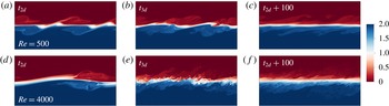
Figure 1 shows contour plots of the density field, on the $x$ – $z$ plane at the spanwise midpoint of the computational domain for simulation ‘H05’ at $Re=500$ (a–c) and simulation ‘H40’ at $Re=4000$ (d–f) at $t_{2d}$ , $t_{3d}$ and $t_{2d}+100$ . Note that, as mentioned earlier in § 2, simulation ‘H05’ includes two wavelengths of the primary HWI due to its horizontal extent being twice the wavelength of the fastest (linear) growing mode. There is no indication of vortex merging due to a subharmonic pairing instability even at $Re$ as low as $Re=500$ (or even lower at $Re=300$ , based on simulation ‘H03’; not shown), let alone at higher Reynolds numbers at which such subharmonic instability has been shown to become increasingly suppressed in flows susceptible to the primary KHI as $Re$ increases (Mashayek & Peltier Reference Mashayek and Peltier2012).

As illustrated in figure 1, the evolution of the high- $Re$ HWI appears to be qualitatively different from the low- $Re$ simulation, although, similarly to previously described low- $Re$ studies (see e.g. Smyth et al. Reference Smyth, Klaassen and Peltier1988), at high $Re$ the development of the primary two-dimensional HWI still includes two counter-propagating waves above and below the shear layer (cf. figure 1 a,d at $t_{2d}$ ). Nevertheless, it appears that at high $Re$ the HWI experiences strong secondary instabilities that trigger turbulence with a much broader range of spatial scales (cf. figure 1 b,e at $t_{3d}$ ). In particular, as we discuss further below, the ensuing turbulence (cf. figure 1 c,f at $t_{2d}+100$ ) is much more vigorous and widespread at higher $Re$ than intermittent and weak ‘wisp’ ejections from interfacial cusps that are characteristic of low- $Re$ HWI and apparent in the upper panels.

Figure 1.

Contour plots of density evolution for simulation ‘H05’ (a–c) and simulation ‘H40’ (d–f) on the $x$ – $z$ plane at the spanwise midpoint of the computational domain at $t=t_{2d}$ , $t_{3d}$ and $t_{2d}+100$ , as defined in the text. While the horizontal extent of these panels illustrates $L_{x}$ , which is almost twice as long in (a–c) as in (d–f), their vertical extent is chosen to result in similar panel aspect ratio and is smaller than $L_{z}$ .

3.1.1 $Re$ effects on the transition phase of HWI

A careful characterisation of the ‘zoo’ of secondary instabilities at high $Re$ that emerge subsequent to the growth of the primary HWI is beyond the scope of the current paper. The classical method of linear stability analysis based on Floquet theory that is employed for similar purposes (by e.g. Klaassen & Peltier Reference Klaassen and Peltier1985, Reference Klaassen and Peltier1989; Mashayek & Peltier Reference Mashayek and Peltier2012; Salehipour et al. Reference Salehipour, Peltier and Mashayek2015) (in the context of KHI) is based on a fundamental assumption of time-scale separation between the slow growth of the primary two-dimensional instability and the fast growth of the inherently three-dimensional secondary instabilities. However, the growth of HWI involves yet a further time scale associated with the oscillatory nature of the oppositely travelling interfacial waves in this initially symmetric flow which thereby may undermine the assumption of time-scale separation. Therefore, as also noted by Smyth (Reference Smyth2006), it is questionable whether a similar tool (see Smyth & Peltier Reference Smyth and Peltier1991) should be employed for analysing the secondary instabilities involved in the three-dimensionalisation of HWI. It would be more natural to utilise adjoint-based methods (see the recent review of Luchini & Bottaro (Reference Luchini and Bottaro2014)), which allow the identification of the most rapidly growing perturbations on a time-varying non-parallel base flow over a finite time horizon. This method has recently proved useful to identify the optimal infinitesimal perturbations that grow on a developing unstratified flow susceptible to a primary KHI, even when the primary instability is varying too rapidly for an assumption of time-scale separation to be valid (see Arratia, Caulfield & Chomaz (Reference Arratia, Caulfield and Chomaz2013) for further details).

Figure 2.

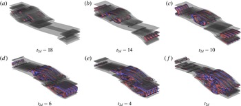
Three-dimensional isosurfaces of streamwise vorticity, $\unicode[STIX]{x1D714}_{x}=-0.25$ (blue) and $\unicode[STIX]{x1D714}_{x}=0.25$ (red) overlaid by an isosurface of spanwise vorticity, $\unicode[STIX]{x1D714}_{y}=0.5$ (grey) for simulation ‘H40’ at $Re=4000$ during one Holmboe wave cycle starting at $t_{2d}-18$ and ending at $t_{2d}$ . The counter-propagating streamwise vortex tubes associated with the secondary shear-aligned convective instability are shown to play a significant role during the transition to turbulence of HWI at this high $Re$ .

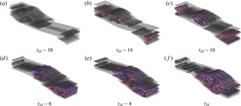
Nevertheless, the three-dimensionalisation of HWI at high $Re$ may be qualitatively investigated by inspecting the vorticity field. Figure 2 illustrates the time evolution of streamwise vorticity isosurfaces with $\unicode[STIX]{x1D714}_{x}=\pm 0.25$ , overlaid (for better visualisation) by an isosurface of spanwise vorticity with $\unicode[STIX]{x1D714}_{y}=0.5$ , during a full cycle of the HWI oscillation that is precursory to $t_{2d}$ . It is quite evident that, at this high $Re$ , familiar vortex structures emerge as robust features of the three-dimensionalisation process of HWI. These counter-rotating shear-aligned rolls of secondary convective instability have been previously identified as a primary catalyst of three-dimensionalisation of KHI at both relatively low- $Re$ (see e.g. Klaassen & Peltier Reference Klaassen and Peltier1985; Caulfield & Peltier Reference Caulfield and Peltier1994, Reference Caulfield and Peltier2000) and high- $Re$ (Mashayek & Peltier Reference Mashayek and Peltier2013; Salehipour et al. Reference Salehipour, Peltier and Mashayek2015) conditions. Similar manifestations of this mode of secondary convective instability have not previously been reported in the literature for HWI, although its weak indications are present at low- $Re$ simulations of Smyth (Reference Smyth2006) (see his figure 10). It is apparent that these counter-rotating convective rolls play a crucial role in the transition of HWI into turbulence at high $Re$ . Thus it appears that the introduction of a further time scale associated with the oscillations of the initially two-dimensional Holmboe waves has not hindered the emergence of the Klaassen–Peltier mode of instability and therefore we conjecture that it continues to be the primary catalyst of transition for the assumed values of $R$ , $Ri_{b}$ and $Pr$ (see table 1).

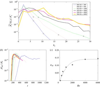
The important role of $Re$ in the emergence of these secondary instabilities, and hence the three-dimensionalisation process, may be quantified by considering the spanwise spectra of the spanwise kinetic energy, $\widehat{\mathscr{K}_{y}^{\prime }}(k_{y},t)$ (2.17), at time $t=t_{2d}$ . Figure 3(a) illustrates the spanwise wavenumber ( $k_{y}$ ) variations of $\widehat{\mathscr{K}_{y}^{\prime }}(k_{y})$ after being normalised by the total spanwise kinetic energy $\mathscr{K}_{y}^{\prime }=(2\unicode[STIX]{x03C0}/L_{y})\sum _{k_{y}}\widehat{\mathscr{K}_{y}^{\prime }}$ for simulations ‘H03’, ‘H05’, ‘H10’, ‘H20’, ‘H40’ and ‘H60’. These simulations cover more than one decade in $Re$ (i.e. $Re=300$ to $6000$ ). Note that, at the time $t=t_{2d}$ , the spanwise kinetic energy is injected at a length scale that is associated with the shear-aligned secondary convective rolls as depicted in figure 2.

Figure 3.

(a) The spanwise spectrum of spanwise kinetic energy, $\widehat{\mathscr{K}_{y}^{\prime }}(k_{y})$ (2.17), at $t=t_{2d}$ . Symbols ‘○’ and ‘▫’ (if available) mark $\ell _{O}$ and $\ell _{K}$ (2.31), respectively. (b) Time evolution of the three-dimensional kinetic energy, $\mathscr{K}_{3d}$ , after being normalised by the initial total kinetic energy $\mathscr{K}_{0}$ for a series of HWI simulations with different values of initial $Re$ (see table 1). The saturation time of two-dimensional primary HWI, $t_{2d}$ , is marked by a ‘ $+$ ’ for each simulation. (c) The $Re$ dependence of $\unicode[STIX]{x1D70E}_{3d}=(1/(2\mathscr{K}_{3d}))\,\text{d}\mathscr{K}_{3d}/\text{d}t$ associated with the growth rate of the three-dimensional perturbations. The dashed curve provides a sigmoid fit for illustrative purposes.

The wavenumber at which the spectra achieve maximum amplitude (i.e. the dominant injection scale) must therefore be attributed to these rolls in the spanwise direction. For example, focusing on simulation ‘H40’, figure 2(f) suggests a wavelength of approximately $\unicode[STIX]{x1D706}=L_{y}/4$ associated with these rolls. This wavelength corresponds to $k_{y}\sim 4\unicode[STIX]{x1D6FF}k_{y}\sim 8$ , which is fairly consistent with figure 3(a) (simulation ‘H40’). Note that, as shown in figure 2, the spanwise structure of these rolls is much more clearly visible at $t<t_{2d}$ and becomes more distorted at $t_{2d}$ , which is why the peak of the spanwise spectra associated with simulation ‘H40’ in figure 3(a) covers a relatively wider range of scales including $k_{y}\sim 8$ .

Figure 3(a) also demonstrates that the dominant injection scale associated with shear-aligned convective rolls shifts towards higher wavenumbers as $Re$ increases (e.g. compare cases ‘H10’, ‘H20’, ‘H40’ and ‘H60’ in figure 3 a). This shift would be manifest physically by an increasingly high number of streamwise rolls as $Re$ increases.

The increase in the dominant spanwise wavenumber of the cross-stream spectra that occurs as a consequence of increasing $Re$ leads to a qualitatively different process of three-dimensionalisation during the transition to the turbulent phase of HWI. This difference may be further demonstrated by inspecting the growth rate of the three-dimensional perturbations, i.e. $\unicode[STIX]{x1D70E}_{3d}=(1/(2\mathscr{K}_{3d}))\,\text{d}\mathscr{K}_{3d}/\text{d}t$ , which assumes $\mathscr{K}_{3d}\propto \exp (2\unicode[STIX]{x1D70E}_{3d}t)$ .

Figure 3(b) illustrates the time dependence of $\mathscr{K}_{3d}$ for simulations with increasing values of $Re$ (from ‘H03’ to ‘H60’), while figure 3(c) plots the inferred $\unicode[STIX]{x1D70E}_{3d}$ as a function of $Re$ . In figure 3(c), $\unicode[STIX]{x1D70E}_{3d}$ is calculated based on the slope of $\mathscr{K}_{3d}$ during its exponential growth stage associated with the emergence of three-dimensional secondary instabilities that is most visible in figure 3(b) at $t<t_{2d}$ (for each simulation in figure 3(b), $t_{2d}$ is marked by a ‘ $+$ ’). Also note that figure 3(c) includes an additional data point indicating $\unicode[STIX]{x1D70E}_{3d}=0$ for $Re=100$ for which $\mathscr{K}_{3d}(t)$ is not shown in figure 3(b). This additional data point is based on simulation ‘H01’ at $Re=100$ for which $\mathscr{K}_{3d}$ does not grow at all. In this case, the two-dimensional oscillating HWI that emerges remains completely two-dimensional until being viscously dissipated entirely.

As suggested by figure 3(c), the growth rate of the three-dimensional perturbations, as measured by $\unicode[STIX]{x1D70E}_{3d}$ , increases nonlinearly with $Re$ and becomes ‘saturated’ for $Re\gtrsim 4000$ . This non-trivial saturation of $\unicode[STIX]{x1D70E}_{3d}$ with respect to $Re$ implies that, for $Re\gtrsim 4000$ , the secondary instabilities become as energetic and vigorous as possible for the given values of $Pr$ , $Ri_{b}$ and $R$ . In other words, $Re=4000$ appears to be sufficiently high (for the fixed set of other input parameters) that the transition phase has become largely $Re$ -independent. The nonlinear dependence of $\unicode[STIX]{x1D70E}_{3d}$ on $Re$ is not a matter of degree, which could have been predicted a priori by linear extrapolation of the result obtained from previous low- $Re$ simulations of HWI (e.g. those of Smyth & Winters (Reference Smyth and Winters2003) and Smyth et al. (Reference Smyth, Carpenter and Lawrence2007)) corresponding to (in our convention) $Re\lesssim 600$ , but is rather evidence of qualitatively different dynamics occurring at sufficiently high $Re$ . This is perhaps unsurprising, as it appears that the flow has passed through a ‘mixing transition’ in the sense of Dimotakis (Reference Dimotakis2005).

3.1.2 $Re$ effects on the turbulent phase of HWI

The flows shown in figure 1 suggested that an increase in $Re$ results in a rich range of vigorous turbulent structures that are in fact mediated primarily by secondary instabilities as shown in figure 2 and quantified in figure 3(a). Furthermore, the growth rate of these three-dimensional secondary instabilities was shown in figure 3(c) to become apparently independent of $Re$ for $Re\gtrsim 4000$ . Yet an outstanding question concerns the extent to which these aforementioned findings regarding the influence of $Re$ on the transition phase would affect the stratified turbulent flow that is induced after the primary HWI collapses. We focus upon this issue in what follows in this section.

The characteristic spectral slope of both horizontal and vertical energy spectra in stratified flows as well as the direction of energy cascade (forward or inverse) has been the focus of much debate and discussion based on observational, theoretical and numerical investigations (see e.g. Lilly Reference Lilly1983; Nastrom & Gage Reference Nastrom and Gage1985; Smyth & Moum Reference Smyth and Moum2000; Billant & Chomaz Reference Billant and Chomaz2001; Laval, McWilliams & Dubrulle Reference Laval, McWilliams and Dubrulle2003; Riley & de Bruyn Kops Reference Riley and de Bruyn Kops2003; Waite & Bartello Reference Waite and Bartello2004; Lindborg Reference Lindborg2006; Brethouwer et al. Reference Brethouwer, Billant, Lindborg and Chomaz2007; Riley & Lindborg Reference Riley and Lindborg2008; Augier, Chomaz & Billant Reference Augier, Chomaz and Billant2012; Bartello & Tobias Reference Bartello and Tobias2013). Specifically, a horizontal $k^{-5/3}$ spectrum has been suggested to characterise stratified turbulent flows with length scales larger than the Ozmidov scale ( $\ell \geqslant \ell _{O}$ ) provided that $Re_{b}\gg 1$ (Lindborg Reference Lindborg2006; Brethouwer et al. Reference Brethouwer, Billant, Lindborg and Chomaz2007). Despite the strongly anisotropic effects of stratification on these larger scales, the horizontal components of a spectrum have been shown to exhibit $-5/3$ power-law scaling that is superficially similar to the ‘inertial range’ of unstratified three-dimensional isotropic turbulence. As one approaches $\ell _{O}$ from larger scales, the suppressing effect of the stratification becomes weaker, and therefore a seamless connection with the classical Kolmogorov-like isotropic turbulence for $\ell <\ell _{O}$ is expected.

Unlike previous numerical studies which have characterised the $k^{-5/3}$ horizontal spectrum (see e.g. Riley & de Bruyn Kops Reference Riley and de Bruyn Kops2003; Augier et al. Reference Augier, Chomaz and Billant2012), we do not focus here on ‘forced’ stratified turbulent flow. Rather, our focus is on the turbulent flow that is produced after a ‘freely’ evolving instability mechanism, such as KHI and HWI, breaks down into turbulence (see e.g. figure 1 b,c,e,f). Furthermore, in this section, we will focus only on spectra of streamwise variability, for two reasons: (i) the computational domain (and hence the wavenumber space) has the largest extent in that direction; and (ii) due to the prevailing shear, the fluctuations are naturally strongest in that direction.

Figure 4.

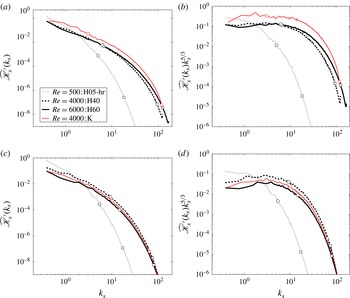
(a,c) Streamwise spectra of $\widehat{\mathscr{K}_{x}^{\prime }}(k_{x},t)$ (2.16) for three simulations ‘H05-hr’, ‘H40’ and ‘K’. (b,d) Compensated streamwise spectra of $\widehat{\mathscr{K}_{x}^{\prime }}(k_{x},t)$ . These spectra are calculated at times (a,b) $t=t_{3d}$ and (c,d) $t_{2d}+100$ . The Ozmidov ( $\ell _{O}$ ) and Kolmogorov ( $\ell _{K}$ ) length scales (see (2.31)) are marked by ‘○’ and ‘▫’, respectively. The effect of $Re$ on the stratified turbulence generated by HWI is illustrated and compared with the spectra of KHI-induced turbulence at a similarly high $Re$ .

Figure 5.

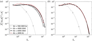
Compensated streamwise spectra of $\widehat{\mathscr{K}_{x}^{\prime }}(k_{x},t)$ (2.16) after being normalised by the total streamwise perturbation kinetic energy $\mathscr{K}_{x}^{\prime }=(2\unicode[STIX]{x03C0}/L_{x})\sum _{k_{x}}\widehat{\mathscr{K}_{x}^{\prime }}$ for simulations ‘H05-hr’, ‘H40’, ‘H60’ and ‘K’. These spectra are calculated at times (a) $t=t_{3d}$ and (b) $t=t_{2d}+100$ . Similar to figure 4, $\ell _{O}$ and $\ell _{K}$ are marked by ‘○’ and ‘▫’, respectively.

Figure 4 compares the streamwise spectra associated with the streamwise perturbation kinetic energy, $\widehat{\mathscr{K}_{x}^{\prime }}(k_{x},t)$ (see (2.16)) in both unscaled and compensated forms. These spectra are calculated at $t=t_{3d}$ (figure 4 a,b) and $t=t_{2d}+100$ (figure 4 c,d) for simulations ‘H05-hr’ (HWI at $Re=500$ ), ‘H40’ (HWI at $Re=4000$ ), ‘H60’ (HWI at $Re=6000$ ) and ‘K’ (KHI at $Re=4000$ ). For consistency, the spatial resolution employed in ‘H05-hr’ is identical to that of ‘H40’ (see table 1), implying an identical resolution also in the Fourier wavenumber space. The Ozmidov ( $\ell _{O}$ ) and Kolmogorov ( $\ell _{K}$ ) length scales (as defined in (2.31)) are also marked on figure 4 by open circles and open squares, respectively (note that, for example, the Ozmidov wavenumber is defined as $k_{O}=1/\ell _{O}$ ). Thus $Re_{b}$ might also be inferred from figure 4 as $Re_{b}=(\ell _{O}/\ell _{K})^{4/3}$ .

There are several interesting findings based on figure 4. Increasing $Re$ dramatically affects the energy spectrum associated with the turbulence induced by HWI. Comparing $\widehat{\mathscr{K}_{x}^{\prime }}(k_{x},t_{3d})$ and $\widehat{\mathscr{K}_{x}^{\prime }}(k_{x},t_{2d}+100)$ for simulations ‘H05-hr’ and ‘H40’ clearly demonstrates the qualitative difference in the streamwise spectra. This suggests that the disordered states shown in figure 1 for these two simulations are qualitatively different in character. As already noted, this is not surprising, as it is consistent with the influential ‘mixing transition’ hypothesis of Dimotakis (Reference Dimotakis2005).

Furthermore, a $-5/3$ spectrum for $\ell \geqslant \ell _{O}$ is only realised if $Re$ is sufficiently high (i.e. $Re\gtrsim 4000$ ). Such a characteristic spectrum of $k_{x}^{-5/3}$ for $\ell \geqslant \ell _{O}$ is especially apparent at $t=t_{3d}$ when $Re_{b}$ is usually largest. Increasing $Re$ from $Re=4000$ to $Re=6000$ also provides a more seamless connection at $\ell _{O}$ between a characteristic $-5/3$ power-law scaling and that of classical Kolmogorov (i.e. isotropic) turbulence, which is again due to its higher $Re_{b}$ value at this time (i.e. $Re_{b}(t_{3d})=38$ versus $Re_{b}(t_{3d})=51$ ). Indeed, for the KHI simulation at $Re=4000$ , this transition at $\ell _{O}$ appears to be smoother, because $Re_{b}(t_{3d})=124$ is higher.

Moreover, it is very interesting to note that the spectra associated with both KHI and HWI become almost indistinguishable for sufficiently high $Re$ when normalised by the total perturbation kinetic energy of the streamwise spectra (i.e. $\mathscr{K}_{x}^{\prime }=(2\unicode[STIX]{x03C0}/L_{x})\sum _{k_{x}}\widehat{\mathscr{K}_{x}^{\prime }}$ ). This striking similarity persists in time during the turbulent stage (cf. figure 5 a,b).

The value of $Re_{b}=(\ell _{O}/\ell _{K})^{4/3}$ (2.30) at $t_{3d}$ quantifies the maximum instantaneous level of turbulence energetics (as measured by turbulent dissipation) relative to the stabilising effects of viscosity and stratification. Based on figure 5(a), for example, the HWI at $Re=500$ produces $Re_{b}(t_{3d})\sim 6$ . Consequently, at this low $Re_{b}$ , the resulting turbulence belongs to a regime that is dominated by molecular viscous effects. In fact, in practice, flows with $Re_{b}>20$ are usually considered to be ‘turbulent’ (Smyth & Moum Reference Smyth and Moum2000), in accord with the arguments of Brethouwer et al. (Reference Brethouwer, Billant, Lindborg and Chomaz2007) for $Re_{b}\gg 1$ . This requirement means that $\ell _{O}$ and $\ell _{K}$ should be sufficiently widely separated for a turbulent cascade to be largely unaffected by both viscosity and stratification. In other words, at lower $Re_{b}$ values, the flow becomes laminar due to the combined suppressing effects of stratification and viscosity.

3.1.3 $Re$ effects on mixing of HWI

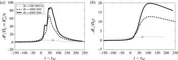
We wish to quantify the effect of Reynolds number on irreversible mixing induced by HWI. The results of simulations ‘H05-hr’ (at $Re=500$ ), ‘H40’ (at $Re=4000$ ) and ‘H60’ (at $Re=6000$ ) are used in figure 6 in order to produce appropriate ‘instantaneous’ and ‘cumulative’ measures of mixing. Specifically, figure 6(a) illustrates the time variation of $\mathscr{M}/D_{p}=K_{\unicode[STIX]{x1D70C}}^{\ast }/\unicode[STIX]{x1D705}$ (see the discussion following (2.24)), which quantifies the instantaneous level of irreversible diapycnal mixing relative to the molecular diffusion rate. In addition, figure 6(b) shows the time dependence of the cumulative irreversible mixing $\mathscr{M}_{c}$ (2.22) that is directly related to the cumulative increase in BPE, in this case with respect to the (notional) cumulative increase associated with the laminar diffusion ( $D_{p}t$ ). For ease of comparison, the abscissa is shifted from $t$ to $t-t_{2d}$ in these panels of figure 6.

Figure 6.

Time dependence for simulations ‘H05-hr’ ( $Re=500$ , dotted), ‘H40’ ( $Re=4000$ , dashed) and ‘H60’ ( $Re=6000$ , solid) of: (a) instantaneous mixing rate, $\mathscr{M}$ (2.18) relative to the laminar diffusion rate $D_{p}$ (2.21); and (b) cumulative irreversible mixing $\mathscr{M}_{c}$ (2.22) normalised by $D_{p}t$ (2.21). The time $t_{3d}$ in both panels is indicated by ‘*’.

For HWI at $Re=500$ (see figure 6 a), $K_{\unicode[STIX]{x1D70C}}^{\ast }$ remains comparable to the molecular diffusivity ( $\unicode[STIX]{x1D705}$ ) throughout its entire life cycle (i.e. its maximum reaches ${\sim}4\unicode[STIX]{x1D705}$ ). This dominance of molecular effects as noted earlier (recall that $Re_{b}(t_{3d})\sim 6$ for this case) is a consequence of the low Reynolds number that has been employed in this simulation. Smyth et al. (Reference Smyth, Carpenter and Lawrence2007) also noted this issue on the basis of their DNS analyses of HWI at $Re=300$ and 600. In addition, based on scaling arguments, they suggested that diapycnal diffusivity would increase linearly with $Re$ . However, this hypothesis is not consistent with our results in figure 6.

For example at $t_{3d}$ (indicated by ‘*’ in figure 6 a), $\mathscr{M}/D_{p}$ (or $K_{\unicode[STIX]{x1D70C}}^{\ast }/\unicode[STIX]{x1D705}$ ) increases nonlinearly with $Re$ (i.e. varies from ${\sim}4$ at $Re=500$ to ${\sim}62$ at $Re=4000$ or to ${\sim}87$ at $Re=6000$ ). Similarly, a cumulative measure of net diapycnal diffusivity, as measured by $\mathscr{M}_{c}/D_{p}t$ in figure 6(b), also suggests a nonlinear increase with respect to $Re$ for the total rise in $\mathscr{M}_{c}/D_{p}t$ . It is apparent that, at $Re=500$ , the total cumulative ‘mixing’ scales with purely laminar diffusion, as the dotted line is close to horizontal, while for simulations at higher $Re$ , the mixing is clearly much more intense and qualitatively different in character. Note that the highest value of $Re$ ( $Re=600$ ) in the DNS analyses of Smyth et al. (Reference Smyth, Carpenter and Lawrence2007) is markedly below the transitional Reynolds number of $Re\approx 4000$ for which (i) the growth rate of secondary instabilities begin to saturate (see figure 3 c) and (ii) the spectrum of streamwise perturbation kinetic energy reveals a $-5/3$ power law for $\ell \geqslant \ell _{O}$ (see e.g. figure 4 b).

3.2 Mixing analysis at high $Re$

In the remainder of this paper, and for convenience, we will entirely focus upon the results of two high- $Re$ simulations, namely ‘H40’ (HWI at $Re=4000$ ) and ‘K’ (KHI at $Re=4000$ ). In addition, for brevity, we will refer to simulation ‘H40’ as simulation ‘H’.

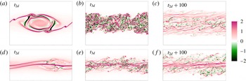
A qualitative comparison of the flow structures resulting from high- $Re$ HWI and KHI may be obtained by inspecting how the primary band of spanwise vorticity in the shear layer evolves in time. For this purpose, figure 7 shows contour plots of the spanwise vorticity, $\unicode[STIX]{x1D714}_{y}$ , on the $x$ – $z$ plane at the spanwise midpoint of the computational domain for simulation ‘K’ (a–c) and simulation ‘H’ (d–f) at the three chosen characteristic times $t_{2d}$ , $t_{3d}$ and $t_{2d}+100$ . Figure 7(a–c) illustrates the typical transition to turbulence mediated by the saturation of a primary KHI subject to strong secondary instabilities (figure 7 a, at $t_{2d}$ ). The saturated KHI then rapidly breaks down into a broad band of turbulence (figure 7 b, at $t_{3d}$ ) that is centred on the ‘overturned’ primary density interface and thus strongly mixes the fluid. Finally, the turbulence gradually decays as the flow relaminarises (figure 7 c, at $t_{2d}+100$ ). The high- $Re$ HWI evolves in a qualitatively different way from the high- $Re$ KHI, as is apparent in figure 7(d–f). Besides the previously known fundamental differences between the linear and nonlinear laminar structure of HWI and KHI (as reviewed briefly in § 1 and explained in depth by, for example, Smyth et al. (Reference Smyth, Klaassen and Peltier1988), Caulfield (Reference Caulfield1994)) that might also be inferred from figure 7(d), it is clear at this high $Re$ that HWI induces a much more long-lived turbulence (figure 7 e at $t_{3d}$ ). Furthermore, unlike KHI-induced mixing that is obtained by overturning of the primary density interface, HWI appears to mix the flow by ‘scouring’ either side of the primary density interface (figure 7 f at $t_{2d}+100$ ). We will focus more on these different mixing mechanisms and their distinct spatial characteristics in the next section.

Figure 7.

Contour plots of the spanwise vorticity ( $\unicode[STIX]{x1D714}_{y}$ ) evolution for simulation ‘K’ (a–c) and simulation ‘H’ (d–f) on the $x$ – $z$ plane at the spanwise midpoint of the computational domain at $t=t_{2d}$ , $t_{3d}$ and $t_{2d}+100$ , as defined in the text.

Figure 8.

(a–c) Vertical structure of horizontally averaged density and velocity profiles ( $\overline{\unicode[STIX]{x1D70C}}$ , $\overline{U}+1$ ) for simulations ‘H’, plotted with thick lines, and ‘K’, plotted with thin lines, at times (a) $t_{2d}$ , (b) $t_{3d}$ and (c) $t_{2d}+100$ . Bottom panels illustrate the time evolution of (d) $R=\ell _{u}/\ell _{\unicode[STIX]{x1D70C}}$ and (e) the bulk Richardson number $Ri_{b}$ , (f) the gradient Richardson number at the interface, $Ri_{g}(0)=RRi_{b}$ , and (g) the Reynolds number $Re$ based on the extended definitions in (2.29). The characteristic times $t_{2d}$ , $t_{3d}$ and $t_{2d}+100$ are marked in (d–g) by ‘ $+$ ’, ‘*’ and ‘ $\times$ ’, respectively.

Figure 9.

Time dependence for simulations ‘H’, plotted with thick lines, and ‘K’, plotted with thin lines, of: (a) the spanwise-averaged kinetic energy $\mathscr{K}_{2d}$ (solid curves) as well as the inherently three-dimensional perturbation kinetic energy $\mathscr{K}_{3d}$ (dashed curves); and (b) changes in the APE ( $\mathscr{P}_{A}$ , solid) and BPE ( $\mathscr{P}_{B}$ , dashed) reservoirs (2.11). For our closed system, the dashed curves also represent the cumulative amount of mixing $\mathscr{M}_{c}(t)$ (2.22).

Figure 10.

Time dependence for simulations ‘H’, plotted with thick lines, and ‘K’, plotted with thin lines, of: (a) irreversible mixing rate, $\mathscr{M}$ , as defined in (2.18) (solid line), viscous dissipation rate $\unicode[STIX]{x1D700}$ , as defined in (2.23) (dashed line); and (b) the buoyancy Reynolds number, $Re_{b}^{\ast }$ , as defined in (2.26).

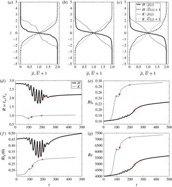
The vertical profiles associated with the horizontally averaged velocity, $\overline{U}(z,t)=\langle u\rangle _{xy}$ , and density profiles, $\overline{\unicode[STIX]{x1D70C}}(z,t)=\langle \unicode[STIX]{x1D70C}\rangle _{xy}$ , of simulations ‘H’ and ‘K’ are illustrated in figure 8(a–c) for the same three characteristic times. Further useful information regarding the temporal evolution of these profiles may be obtained by using the generalised time-dependent forms of $R(t)$ , $Ri_{b}(t)$ , $Ri_{g}(0,t)=RRi_{b}(t)$ and $Re(t)$ as defined in (2.29). These time-dependent quantities are shown in figure 8(d–g) and characterise the evolving shear and density layers associated with KHI and HWI. While the ratio $R(t)$ remains ${\sim}1$ for KHI, it decreases slightly from its initial value of $\sqrt{Pr}\sim 2.8$ (see table 1) to ${\sim}2.2$ for HWI. Although the overall thickness of the shear and stratified layers, as characterised by $\ell _{u}$ and $\ell _{\unicode[STIX]{x1D70C}}$ (2.28), both increase in time for both KHI and HWI (see the vertical profiles in figure 8 a–c), the two scales expand differently in the case of HWI. In particular, the overall expansion of the density layer in HWI is greater than that of the shear layer (hence a decrease in $R$ ). In addition, although both simulations ‘K’ and ‘H’ begin with identical initial values of $Ri_{b}=0.16$ and $Re=4000$ , the final values of these quantities differ noticeably. Both $Ri_{b}$ and $Re$ become greater for KHI than HWI because the shear layer thickness $\ell _{u}$ increases more significantly in the flow susceptible to KHI.

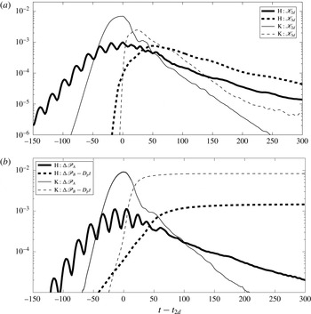
Next we consider quantitatively the energetics of simulations ‘H’ and ‘K’. In figure 9(a) we plot the time dependence of $\mathscr{K}_{2d}$ (solid curve) and $\mathscr{K}_{3d}$ (dashed curve), while in figure 9(b) we plot the time dependence of the change of the BPE and APE energy reservoirs relative to their initial values (e.g. $\unicode[STIX]{x0394}\mathscr{P}_{B}=\mathscr{P}_{B}(t)-\mathscr{P}_{B}(0)$ ) with the purely diffusive component subtracted for BPE. Note that $\unicode[STIX]{x0394}\mathscr{P}_{B}=\mathscr{M}_{c}+D_{p}t$ , as shown in (2.22). The slower and oscillatory nature of the initial growth rate of the HWI, and the smaller maximum amplitude of both the primary instability and the ensuing turbulence by comparison with the KHI, are all apparent in figure 9(a). The oscillations of $\mathscr{K}_{2d}$ are also manifest in the time variations of $R$ and $Ri_{g}(0)$ in figure 8 and $\mathscr{P}_{A}$ in figure 9(b). The oscillatory variations of $\mathscr{P}_{A}$ are nevertheless directly out of phase with $\mathscr{K}_{2d}$ . This anticorrelated time lag is due to the reversible exchanges between $\mathscr{K}_{2d}$ and $\mathscr{P}$ that are stored in the form of $\mathscr{P}_{A}$ . Based on $\mathscr{K}_{3d}$ in figure 9(a), it is also clear that the three-dimensional turbulent motions, and presumably the associated irreversible mixing for the HWI, not only arise later (relative to $t_{2d}$ ) but are also longer-lived.

The cumulative amount of turbulent mixing, $\mathscr{M}_{c}$ (2.22), that is manifested here as the total rise in BPE is approximately five times more for the KHI compared to the HWI. This higher $\mathscr{M}_{c}$ for the KHI is primarily due to the associated extremely rapid rise of BPE between $t_{2d}$ and $t_{3d}$ , which is also synchronised with a rapid and significant decay of APE. Indeed, for the KHI, the maximum $\mathscr{P}_{A}$ is also substantially larger than for the HWI, due to the fact that the KHI overturns the density interface, thus substantially increasing the potential energy of the system through vigorous stirring. The decrease in APE from its large value occurs as a result of a sudden ‘burst’ of turbulence due to the collapse of the KHI overturn, a process that is inherently absent in the case of HWI, where $\mathscr{P}_{A}$ is increased substantially due to ‘scouring’ of the interface by propagating vortices, leading to the characteristic cusped waves of the finite-amplitude manifestation of the HWI. Indeed, HWI involves a slow and gradual rise (or decay) of BPE (or APE) as shown in figure 9(b). We will attribute these differences below to the different mixing mechanics and localisation involved in KHI and HWI.

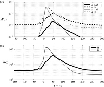
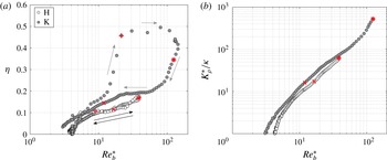
Figure 10(a,b) illustrates the time dependence of the instantaneous values of irreversible mixing rate, $\mathscr{M}$ (as defined in (2.18)), total viscous dissipation, $\unicode[STIX]{x1D700}$ (as defined in (2.23)), and the buoyancy Reynolds number, $Re_{b}^{\ast }$ (as defined in (2.26)). Furthermore, in figure 11(a,b) we plot the $Re_{b}^{\ast }$ dependence of the irreversible mixing efficiency, $\unicode[STIX]{x1D702}$ (as defined in (2.27)), and the irreversible diapycnal diffusivity, $K_{\unicode[STIX]{x1D70C}}^{\ast }$ (as defined in (2.24)). As in figure 8, and for reference, the times $t_{2d}$ (marked by ‘ $+$ ’), $t_{3d}$ (marked by ‘*’) and $t=t_{2d}+100$ (marked by ‘ $\times$ ’) associated with the panels of figure 7 are also indicated in figure 11(a,b). Note that, while figure 11(a) illustrates the entire life cycle of HWI and KHI, figure 11(b) only shows data associated with times subsequent to $t_{3d}$ , after which the flow may be described as three-dimensionally turbulent.

Figure 11.

Variation with $Re_{b}^{\ast }$ for simulation ‘H’ (white circles) and simulation ‘K’ (grey circles) of: (a) the irreversible mixing efficiency, $\unicode[STIX]{x1D702}$ , as defined in (2.27) for the entire life cycle of HWI and KHI; and (b) the irreversible diapycnal diffusivity, $K_{\unicode[STIX]{x1D70C}}^{\ast }$ , as defined in (2.24) for $t\geqslant t_{3d}$ . The data corresponding to times $t_{2d}$ (marked by ‘ $+$ ’), $t_{3d}$ (marked by ‘*’) and $t=t_{2d}+100$ (marked by ‘ $\times$ ’) are also indicated. The direction of time evolution is also indicated by arrows in (a).

The aforementioned longevity of three-dimensional turbulent motions in the HWI compared to KHI is also evident in figure 10(a,b). Despite their earlier vigour in KHI, the irreversible mixing ( $\mathscr{M}$ ), turbulent dissipation ( $\unicode[STIX]{x1D700}$ ) and the buoyancy Reynolds number ( $Re_{b}$ ) associated with HWI surpass those of KHI at equivalent times after $t_{2d}$ . Therefore, this long-lived turbulent activity suggests that it is possible for flows susceptible to HWI to induce non-trivial amounts of mixing associated with inherently turbulent processes. This suggestion is confirmed by the data presented in figure 11(a,b).

Although the irreversible mixing associated with the HWI for given $Re_{b}^{\ast }$ is less efficient than the mixing associated with the KHI, through much of the life cycle the difference is modest, once the highest $Re_{b}^{\ast }$ (and earliest) stage of simulation ‘K’ is eliminated (as is done in figure 11(b) by including the data associated with $t\geqslant t_{3d}$ ). This early, typically very efficient, mixing stage is associated with the large-scale overturning of the density interface by the primary KHI, which does not arise in the evolution of the HWI. In this regard, it is very interesting to note that the mixing efficiency of HWI proceeds in time along a similar trajectory for which the later-time mixing efficiency $\unicode[STIX]{x1D702}(t\geqslant t_{3d})$ closely follows the early-time $\unicode[STIX]{x1D702}(t<t_{3d})$ . This behaviour differs completely from that of $\unicode[STIX]{x1D702}(t)$ during the KHI life cycle in which the flow evolution executes a wide loop in $Re_{b}{-}\unicode[STIX]{x1D702}$ space. Furthermore, the KHI exhibits mixing efficiencies much larger than the canonical value of $\unicode[STIX]{x1D702}\leqslant 1/6$ ( $\unicode[STIX]{x1D6E4}\leqslant 0.2$ ) as proposed by Osborn (Reference Osborn1980), precisely because of this large-scale stirring at relatively early times, while the HWI behaviour (possibly fortuitously) appears to be much more consistent with this classical model throughout its turbulent life cycle. A key open question, therefore, is under what conditions KHI-like overturning or HWI-like scouring might be typical of real-world mixing processes.

Nevertheless, as is apparent in figure 11(b), once both flows have broken down into smaller-scale turbulence and after the three-dimensional motions have saturated (i.e. for $t\geqslant t_{3d}$ ), the turbulent diapycnal diffusivity $K_{\unicode[STIX]{x1D70C}}^{\ast }$ (defined in (2.24)) over the entire turbulent phase is actually rather similar between the two simulations. Indeed, at the highlighted time $t_{2d}+100$ shown in figure 7(c,f), $K_{\unicode[STIX]{x1D70C}}^{\ast }$ is actually larger in simulation ‘H’. Therefore, provided the flow is at sufficiently high $Re$ , the irreversible mixing associated with HWI involves a qualitatively different picture compared to the low- $Re$ characteristic ‘wisping’ from interfacial cusps; a mixing that is no longer dominated by molecular viscous effects. This finding strongly supports the conjecture that the HWI-induced mixing is geophysically relevant and hence should be considered as a possibly important route to turbulence in stratified flows.

3.3 Mixing mechanics and localisation

Figure 12.

Time dependence of vertical profiles of horizontally averaged (a,b) $\overline{N^{2}}(z,t)$ , (c,d) $\log \overline{\unicode[STIX]{x1D700}}(z,t)$ , (e,f) $\log \overline{\unicode[STIX]{x1D712}}(z,t)$ , (g,h) $\log \overline{Re_{b}}(z,t)$ and (i,j) $\log K_{\unicode[STIX]{x1D70C}}^{cox}(z,t)/\unicode[STIX]{x1D705}$ as defined in (3.1) for simulation ‘K’ (a,c,e,g,i) and simulation ‘H’ (b,d,f,h,j). For details of the colour map with monotonically increasing brightness, see Green (Reference Green2011).

To gain a more complete understanding of the spatiotemporal structure of the qualitatively different mixing mechanisms associated with the ‘overturning’ of the KHI and the ‘scouring’ of the HWI, in figure 12 we plot the time evolution of five horizontally averaged quantities, i.e. the horizontally averaged buoyancy frequency $\overline{N^{2}}(z,t)$ , dissipation rate $\overline{\unicode[STIX]{x1D700}}(z,t)$ , scalar variance dissipation rate $\overline{\unicode[STIX]{x1D712}}(z,t)$ , buoyancy Reynolds number $\overline{Re_{b}}(z,t)$ and Cox number $C$ , defined as

(3.1)

$$\begin{eqnarray}\displaystyle \left.\begin{array}{@{}c@{}}\displaystyle \overline{N^{2}}(z,t)=-Ri_{b}\frac{\text{d}\overline{\unicode[STIX]{x1D70C}}}{\text{d}z},\quad \overline{\unicode[STIX]{x1D700}}(z,t)=\frac{2}{Re}\overline{(\unicode[STIX]{x1D634}_{ij}\unicode[STIX]{x1D634}_{ij})},\quad \overline{\unicode[STIX]{x1D712}}(z,t)=\frac{2}{Re\,Pr}\overline{|\unicode[STIX]{x1D735}\unicode[STIX]{x1D70C}^{\prime }|^{2}},\\ \displaystyle \overline{Re_{b}}(z,t)=\frac{\overline{\unicode[STIX]{x1D700}}(z,t)}{\unicode[STIX]{x1D708}\overline{N^{2}}(z,t)},\quad C=\frac{K_{\unicode[STIX]{x1D70C}}^{cox}}{\unicode[STIX]{x1D705}}=\frac{\overline{|\unicode[STIX]{x1D735}\unicode[STIX]{x1D70C}^{\prime }|^{2}}}{(\text{d}\overline{\unicode[STIX]{x1D70C}}/\text{d}z)^{2}}.\end{array}\right\} & & \displaystyle\end{eqnarray}$$

In these expressions, $\unicode[STIX]{x1D70C}^{\prime }$ denotes the perturbation from the horizontally averaged mean density field $\overline{\unicode[STIX]{x1D70C}}$ (i.e. $\unicode[STIX]{x1D70C}^{\prime }(\boldsymbol{x},t)=\unicode[STIX]{x1D70C}(\boldsymbol{x},t)-\overline{\unicode[STIX]{x1D70C}}(z,t)$ ). The Cox number $C$ is an appropriately normalised measure of diapycnal diffusivity, $K_{\unicode[STIX]{x1D70C}}^{cox}$ (Salehipour & Peltier Reference Salehipour and Peltier2015), as approximated by the formulation of Osborn & Cox (Reference Osborn and Cox1972). In each panel, the horizontal time axis is, as usual, shifted to $t-t_{2d}$ for ease of comparison between the two simulations, with the data from simulation ‘K’ being plotted in the left column and the data from simulation ‘H’ being plotted in the right column.

The qualitatively different character of the turbulence and ensuing mixing is immediately apparent in figure 12(a,b), showing $\overline{N^{2}}(z,t)$ . The overturning associated with the KHI induces a relatively well-mixed region at the midpoint of the flow bounded by two regions of heightened gradient, while the scouring associated with the HWI is not able to destroy the fundamentally two-layer character of the density distribution, and the maximum density gradient clearly remains at its initial location at the midpoint of the shear layer. Interestingly, the turbulence, characterised by $\overline{\unicode[STIX]{x1D700}}$ and $\overline{\unicode[STIX]{x1D712}}$ , is for both simulations centred on the midpoint of the shear layer. However, the KHI has a much more intense and transient ‘burst’ of turbulence intensity spread over a much broader vertical extent, undoubtedly associated with the breakdown of the primary overturning billow shown in figure 7(a), while the HWI exhibits a much longer period of substantial turbulent activity, which is also much more strongly localised in the vicinity of the primary density interface. This difference in the duration of the period of intense turbulent activity between the two simulations reported here is real, since we deliberately choose the (dimensional) advective time scale $d/U_{0}$ to be the same in each simulation.

Taken together, the differences between the spatiotemporal distribution of the stratification and the turbulence lead to major qualitative differences in the properties of the irreversible mixing, as shown in figure 12(g–j). Although $\overline{\unicode[STIX]{x1D700}}$ is widely spread vertically for simulation ‘K’, the buoyancy Reynolds number is typically largest at the midpoint of the shear layer since the buoyancy frequency is in turn subsequently intensified at the periphery. Furthermore, for simulation ‘K’, $\overline{Re_{b}}$ decays quite rapidly in time because $\overline{\unicode[STIX]{x1D700}}$ is elevated only over a relatively short time. Similarly, the ultimate diapycnal diffusivity (as parametrised by the Cox number $C$ ) is most intense for a relatively short time and in the immediate vicinity of the initial primary density interface for simulation ‘K’.

On the other hand, the less intense, but more temporally extended, turbulence associated with the HWI does not disrupt the buoyancy frequency distribution sufficiently to increase $\overline{N^{2}}$ significantly away from the initial density interface. Therefore, as is apparent in figure 12(h), $\overline{Re_{b}}$ develops a distinctive twin lobe structure, with long-lived maxima at the periphery of the shear layer. This long-lived twin-lobed structure is even more pronounced for the Cox number, demonstrating not only that flows susceptible to HWI can induce substantial irreversible mixing, but also that such non-trivial irreversible mixing does not require vigorous precursory stirring of a ‘weak’ density interface (i.e. low $Ri_{g}(0)$ ) by an overturning billow but rather can arise due to the cumulative effect of individually smaller-scale eddying motions ‘scouring’ fluid either side of a ‘strong’ density interface.

The more long-lived turbulence induced by HWI as well as its sustained levels of strong mixing discussed in this paper for flows at high $Re$ should not be attributed to the slower linear growth rate of the primary HWI (relative to KHI). Based on their low- $Re$ DNS analyses of KHI and HWI, Smyth & Winters (Reference Smyth and Winters2003) and Smyth et al. (Reference Smyth, Carpenter and Lawrence2007) found enhanced cumulative mixing due to HWI and thereby associated that with the slower growth rate of the primary HWI. While this argument may be valid for quasi-laminar flows dominated by molecular viscous effects, it does not explain the longevity of our high- $Re$ turbulent mixing events induced by HWI. Note that the primary instability saturates at $t_{2d}$ , which obviously differs for HWI and KHI. Nonetheless, in all the foregoing analysis, we have compensated for this difference by considering times relative to $t_{2d}$ (i.e. $t-t_{2d}$ ). Alternatively, this long-lived and sustained turbulent mixing of high- $Re$ HWI can be explained by recalling the differences between HWI and KHI concerning the mechanics and localisation of mixing as discussed in this section. In particular, the density interface of HWI remains robust even after the primary wave ‘breaks’, which contrasts with the overturned density interface of KHI. Furthermore, this robust interface is being ‘scoured’ from above and below and therefore mixing is displaced away from the interface itself and is localised in those regions where density stratification is relatively weak. In other words, turbulence is not required to ‘overturn’ a strong density interface in order for mixing to occur, and so it is possible for such ‘scouring’-related mixing to be sustained for a longer period of time.

4 Conclusions

We have considered the transition to turbulence and subsequent irreversible mixing of a stably stratified parallel shear flow with a sufficiently sharp density interface centred within the associated shear layer so that it is linearly unstable to counter-propagating Holmboe wave instabilities (HWI). For comparison, we have considered another stably stratified parallel shear flow with the same bulk Richardson number $Ri_{b}$ (as defined in (1.3)) but a more diffuse density interface that is linearly unstable to the classical Kelvin–Helmholtz instability (KHI).

We have shown that the flow Reynolds number has a significant effect not only on the transition phase to turbulence but also on the spectral properties of the induced stratified turbulence as well as its mixing properties. At sufficiently high $Re$ , either one of the two oppositely propagating modes of HWI hosts a clear emergence of shear-aligned secondary convective instability that play a crucial role in three-dimensionalisation of the flow. Apparently, this is the same mode of secondary instability initially discovered by Klaassen & Peltier (Reference Klaassen and Peltier1985, Reference Klaassen and Peltier1989) to govern the transition process in density-stratified Kelvin–Helmholtz billows. The dominant injection length scale in the spanwise direction, associated with this mode of secondary instability, decreases as $Re$ increases, leading to a higher number of prominent streamwise vortex rolls. Furthermore, the growth rate of three-dimensional secondary instabilities increases nonlinearly as $Re$ increases and appears to become saturated for $Re\gtrsim 4000$ .

We have also shown that, at our choice of sufficiently high $Re$ , HWI induces vigorous turbulence and mixing that is clearly different in character from previous studies at lower $Re$ (cf. e.g. Smyth & Winters Reference Smyth and Winters2003; Smyth et al. Reference Smyth, Carpenter and Lawrence2007). In particular, the streamwise spectrum of streamwise perturbation kinetic energy reveals a $-5/3$ power law for scales greater than the Ozmidov scale provided that $Re$ is higher than a ‘transitional’ Reynolds number of $Re\approx 4000$ . This spectral behaviour is in accord with previous theoretical and numerical studies of stratified turbulence (e.g. Brethouwer et al. Reference Brethouwer, Billant, Lindborg and Chomaz2007) and is also evident for the turbulent flow produced by high- $Re$ KHI. In fact the normalised spectra of high- $Re$ KHI- and HWI-induced turbulence become very similar and almost indistinguishable at later times during the fully developed stage when scaled by total perturbation kinetic energy. Insofar as irreversible mixing due to HWI is concerned, as $Re$ increases, the cumulative and instantaneous measures of mixing are both enhanced significantly and in a nonlinear fashion such that the high- $Re$ results would not have been predictable on the basis of linear extrapolation of previous low- $Re$ simulations.

The high- $Re$ breakdown to turbulence of HWI induces non-trivial instantaneous irreversible mixing rates that for a given $Re_{b}$ are comparable in magnitude to the mixing associated with the equivalent fully turbulent flow produced by KHI, but yet result in a reduced amount of cumulative mixing compared to that due to KHI. Both HWI and KHI flows at high $Re$ exhibit vigorous irreversible diapycnal mixing with similar efficiencies and diapycnal diffusivities, particularly after the complete destruction of the primary KHI billow (see figure 11 a,b). Nevertheless, the total amount of cumulative mixing (or the total rise in BPE) gained throughout the life cycle of the high- $Re$ HWI is approximately five times less than that of KHI. This elevated amount of cumulative mixing in KHI should be attributed to the sudden ‘burst’ of turbulence due to the collapse of the overturned KHI billow. As a consequence of this abrupt breakdown event, a substantial amount of energy is exchanged irreversibly from APE into BPE. A similar process is mechanistically irrelevant to the HWI as the APE reaches a much reduced maximum value compared to the flow susceptible to the KHI due to the absence of large-scale overturning. Therefore the energy transfer between APE and BPE occurs at a much more modest rate, resulting in a reduced rise in BPE.

In fact, the character and spatial structure of the turbulence and mixing are completely different for the flows susceptible to KHI and HWI. The mixing associated with the HWI is both much more long-lived than in the flow associated with the KHI, and also does not lead to a well-mixed middle layer, as the mixing is associated with multiple smaller ‘scouring’ events on either side of the primary density interface. Crucially, we have demonstrated that flows susceptible to HWI can be substantial sources of energetic turbulent mixing if their Reynolds number is sufficiently high, even when the gradient Richardson number $Ri_{g}(0)\simeq 0.45$ in the vicinity of the density interface is ‘strong’.

Indeed, this demonstration suggests at least three interesting further avenues for research. First, since ‘scouring’ has been shown to be a mixing mechanism that is essentially as efficient and significant as ‘overturning’, it will be natural to investigate whether any connections can be established with research on unstratified flows of the relative importance of large-scale ‘engulfment’ to small-scale ‘nibbling’ at interfaces between turbulent and non-turbulent regions (see e.g. Westerweel et al. Reference Westerweel, Fukushima, Pedersen and Hunt2005)). Second, we have shown by example that ‘strong’ turbulence and mixing can occur in flows susceptible to HWI at sufficiently high $Re$ , but it would be of interest to undertake an exhaustive (and computationally exceptionally demanding) parameter study, varying $Re$ , $Ri_{b}$ , $Pr$ and $R$ in realistic ranges to obtain more complete knowledge of the characteristic energetic and spectral properties of stratified shear turbulence associated with ‘sharp’ density interfaces. The results of such a parameter study, especially of flows under strong stratification, should yield further means of improving the recent multi-parameter characterisation of mixing efficiency (i.e. $\unicode[STIX]{x1D702}=f(Ri_{b},Re_{b})$ ) by Salehipour et al. (Reference Salehipour, Peltier, Whalen and MacKinnon2016), which relies entirely on the direct numerical simulation of KHI. Finally, similar studies of HWI may provide insight into outstanding open questions in the broader field of stratified turbulence research, where evidence is mounting that layering is generic, characterised by profoundly anisotropic velocity and density distributions with relatively deep, relatively well-mixed layers separated by relatively thin and sharp interfaces with relatively high density gradients (see e.g. Brethouwer et al. Reference Brethouwer, Billant, Lindborg and Chomaz2007)). We hypothesise that ‘scouring’ mixing associated with high-Reynolds-number Holmboe wave instability, which relies for its initial growth on sharp density interfaces, may be central to the dynamics of such geophysically important and turbulently layered flows, and it is our intention to report on our investigation of these three research avenues in due course.

Acknowledgements

The authors would like to acknowledge the constructive comments of the referees. This research has been conducted in part while H.S. visited DAMTP, University of Cambridge. H.S. is grateful to the David Crighton Fellowship from DAMTP. All the computations were performed on the BG/Q supercomputer of SOSCIP (the Southern Ontario Smart Computing Innovation Platform), which is hosted by the University of Toronto. The research activity of C.P.C. is supported by EPSRC Programme Grant EP/K034529/1 entitled ‘Mathematical Underpinning of Stratified Turbulence’. The research of W.R.P. at the University of Toronto is supported by NSERC Discovery Grant A9627. The data for the initial conditions for the various simulations reported in this paper are made available at http://dx.doi.org/10.17863/CAM.699.

Appendix. A note on DNS resolution

The reader is referred to Salehipour et al. (Reference Salehipour, Peltier and Mashayek2015) (and the references therein) for a more detailed discussion regarding the resolution requirements of the DNS analyses that we have conducted using Nek5000. Nevertheless, here we note that the perturbation kinetic energy spectra, $\widehat{\mathscr{K}_{x}^{\prime }}(k_{x})$ (see (2.16)) and $\widehat{\mathscr{K}_{y}^{\prime }}(k_{y})$ (see (2.17)), remain uninfluenced by a significant increase in the spatial resolution.

This is illustrated in figure 13, which compares the spectra at $t=t_{3d}$ after being normalised by the total perturbation kinetic energy of the spectrum associated with the streamwise and spanwise directions, respectively. For this purpose, simulations ‘H05’ and ‘H05-hr’ have been employed. These two cases share an identical initial $Re$ of $Re=500$ but the latter case resolves spatial scales approximately five times smaller.

Figure 13.

Comparing the effect of grid resolution on the spectral representation of the perturbation kinetic energy at $t=t_{3d}$ by employing simulations ‘H05’ and ‘H05-hr’ (both at $Re=500$ , see table 1). (a) Normalised streamwise spectra of streamwise perturbation kinetic energy, $\widehat{\mathscr{K}_{x}^{\prime }}(k_{x})/\mathscr{K}_{x}^{\prime }$ (see (2.16)). (b) Normalised spanwise spectra of spanwise perturbation kinetic energy, $\widehat{\mathscr{K}_{y}^{\prime }}(k_{y})/\mathscr{K}_{y}^{\prime }$ (see (2.17)). Symbols ‘○’ and ‘▫’ mark $\ell _{O}$ and $\ell _{K}$ , respectively.

The smallest scale for flows with $Pr>1$ is the Batchelor length scale, $\ell _{B}=Pr^{-1/2}\ell _{K}$ . While $\ell _{K}$ is clearly resolved in simulation ‘H05’ and ‘H05-hr’, $\ell _{B}\sim 0.35\ell _{K}$ is only resolved in simulation ‘H05-hr’ and is indeed over-resolved. Nonetheless, it is generally accepted that a reliable DNS analysis must resolve scales down to 3–6 times the dissipation scale (equal to $\ell _{B}$ in these cases with $Pr>1$ ), which is respected consistently in the construction of all DNS cases listed in table 1. The blips at the tail of the spectrum, evident in figure 13(a), are associated with the cut-off Nyquist frequency.

References

Alexakis, A. 2005 On Holmboe’s instability for smooth shear and density profiles. Phys. Fluids 17 (8), 084103.CrossRef Google Scholar

Arratia, C., Caulfield, C. P. & Chomaz, J.-M. 2013 Transient perturbation growth in time-dependent mixing layers. J. Fluid Mech. 717, 90–133.Google Scholar

Augier, P., Chomaz, J.-M. & Billant, P. 2012 Spectral analysis of the transition to turbulence from a dipole in stratified fluid. J. Fluid Mech. 713, 86–108.CrossRef Google Scholar

Bartello, P. & Tobias, S. M. 2013 Sensitivity of stratified turbulence to the buoyancy Reynolds number. J. Fluid Mech. 725, 1–22.Google Scholar

Billant, P. & Chomaz, J.-M. 2001 Self-similarity of strongly stratified inviscid flows. Phys. Fluids 13 (6), 1645–1651.CrossRef Google Scholar

Brethouwer, G., Billant, P., Lindborg, E. & Chomaz, J.-M. 2007 Scaling analysis and simulation of strongly stratified turbulent flows. J. Fluid Mech. 585, 343–368.Google Scholar

Carpenter, J. R., Lawrence, G. A. & Smyth, W. D. 2007 Evolution and mixing of asymmetric Holmboe instabilities. J. Fluid Mech. 582, 103–132.Google Scholar

Carpenter, J. R., Tedford, E. W., Rahmani, M. & Lawrence, G. A. 2010 Holmboe wave fields in simulation and experiment. J. Fluid Mech. 648, 205–223.Google Scholar

Caulfield, C. P. 1994 Multiple linear instability of a layered stratified shear flow. J. Fluid Mech. 258, 155–285.Google Scholar

Caulfield, C. P. & Peltier, W. R. 1994 Three-dimensionalization of the stratified mixing layer. Phys. Fluids 6, 3803–3805.Google Scholar

Caulfield, C. P. & Peltier, W. R. 2000 The anatomy of the mixing transition in homogeneous and stratified free shear layers. J. Fluid Mech. 413, 1–47.Google Scholar

Dimotakis, P. E. 2005 Turbulent mixing. Annu. Rev. Fluid Mech. 37, 329–356.Google Scholar

Fischer, P. F. 1997 An overlapping Schwarz method for spectral element solution of the incompressible Navier–Stokes equations. J. Comput. Phys. 133 (1), 84–101.Google Scholar

Green, D. A. 2011 A colour scheme for the display of astronomical intensity images. Bull. Astron. Soc. India 39, 289–295.Google Scholar

Hogg, A. McC. & Ivey, G. N. 2003 The Kelvin–Helmholtz to Holmboe instability transition in stratified exchange flows. J. Fluid Mech. 477, 339–362.Google Scholar

Holmboe, J. 1962 On the behaviour of symmetric waves in stratified shear layers. Geophys. Publ. 24, 67–113.Google Scholar

Ivey, G. N., Winters, K. B. & Koseff, J. R. 2008 Density stratification, turbulence, but how much mixing? Annu. Rev. Fluid Mech. 40 (1), 169–184.Google Scholar

Klaassen, G. P. & Peltier, W. R. 1985 The onset of turbulence in finite amplitude Kelvin–Helmholtz billows. J. Fluid Mech. 155, 1–35.CrossRef Google Scholar

Klaassen, G. P. & Peltier, W. R. 1989 The role of transverse secondary instabilities in the evolution of free shear layers. J. Fluid Mech. 202, 367–402.Google Scholar

Laval, J.-P., McWilliams, J. C. & Dubrulle, B. 2003 Forced stratified turbulence: successive transitions with Reynolds number. Phys. Rev. E 68 (3), 036308.Google Scholar

Lilly, D. K. 1983 Stratified turbulence and the mesoscale variability of the atmosphere. J. Atmos. Sci. 40 (3), 749–761.Google Scholar

Lindborg, E. 2006 The energy cascade in a strongly stratified fluid. J. Fluid Mech. 550, 207–242.Google Scholar

Lorenz, E. N. 1955 Available potential energy and the maintenance of the general circulation. Tellus 7, 157–167.CrossRef Google Scholar

Luchini, P. & Bottaro, A. 2014 Adjoint equations in stability analysis. Annu. Rev. Fluid Mech. 46 (1), 493.Google Scholar

Mashayek, A., Caulfield, C. P. & Peltier, W. R. 2013 Time-dependent, non-monotonic mixing in stratified turbulent shear flows: implications for oceanographic estimates of buoyancy flux. J. Fluid Mech. 736, 570–593.Google Scholar

Mashayek, A. & Peltier, W. R. 2012 The ‘zoo’ of secondary instabilities precursory to stratified shear flow transition. Part 1. Shear aligned convection, pairing, and braid instabilities. J. Fluid Mech. 708, 5–44.Google Scholar

Mashayek, A. & Peltier, W. R. 2013 Shear induced mixing in geophysical flows: does the route to turbulence matter to its efficiency? J. Fluid Mech. 725, 216–261.Google Scholar

Meyer, C. R. & Linden, P. F. 2014 Stratified shear flow: experiments in an inclined duct. J. Fluid Mech. 753, 242–253.Google Scholar

Nastrom, G. D. & Gage, K. S. 1985 A climatology of atmospheric wavenumber spectra of wind and temperature observed by commercial aircraft. J. Atmos. Sci. 42 (9), 950–960.2.0.CO;2>CrossRef Google Scholar

Osborn, T. R. 1980 Estimates of the local rate of vertical diffusion from dissipation measurements. J. Phys. Oceanogr. 10, 83–89.Google Scholar

Osborn, T. R. & Cox, C. S. 1972 Oceanic fine structure. Geophys. Astrophys. Fluid Dyn. 3 (1), 321–345.CrossRef Google Scholar

Peltier, W. R. & Caulfield, C. P. 2003 Mixing efficiency in stratified shear flows. Annu. Rev. Fluid Mech. 35, 135–167.CrossRef Google Scholar

Riley, J. J. & de Bruyn Kops, S. M. 2003 Dynamics of turbulence strongly influenced by buoyancy. Phys. Fluids 15, 2047–2059.CrossRef Google Scholar

Riley, J. J. & Lindborg, E. 2008 Stratified turbulence: a possible interpretation of some geophysical turbulence measurements. J. Atmos. Sci. 65 (7), 2416–2424.Google Scholar

Salehipour, H. & Peltier, W. R. 2015 Diapycnal diffusivity, turbulent Prandtl number and mixing efficiency in Boussinesq stratified turbulence. J. Fluid Mech. 775, 464–500.Google Scholar

Salehipour, H., Peltier, W. R. & Mashayek, A. 2015 Turbulent diapycnal mixing in stratified shear flows: the influence of Prandtl number on mixing efficiency and transition at high Reynolds number. J. Fluid Mech. 773, 178–223.Google Scholar

Salehipour, H., Peltier, W. R., Whalen, C. B. & MacKinnon, J. A. 2016 A new characterization of the turbulent diapycnal diffusivities of mass and momentum in the ocean. Geophys. Res. Lett. 43, 3370–3379.Google Scholar

Smyth, W. D. 2006 Secondary circulations in Holmboe waves. Phys. Fluids 18 (6), 064104.Google Scholar

Smyth, W. D., Carpenter, J. R. & Lawrence, G. A. 2007 Mixing in symmetric Holmboe waves. J. Phys. Oceanogr. 37, 1566–1583.Google Scholar

Smyth, W. D., Klaassen, G. P. & Peltier, W. R. 1988 Finite amplitude Holmboe waves. Geophys. Astrophys. Fluid Dyn. 43 (2), 181–222.Google Scholar

Smyth, W. D. & Moum, J. N. 2000 Length scales of turbulence in stably stratified mixing layers. Phys. Fluids 12, 1327.CrossRef Google Scholar

Smyth, W. D. & Peltier, W. R. 1989 The transition between Kelvin–Helmholtz and Holmboe instability: an investigation of the overreflection hypothesis. J. Atmos. Sci. 46 (24), 3698–3720.Google Scholar

Smyth, W. D. & Peltier, W. R. 1991 Instability and transition in finite amplitude Kelvin–Helmholtz and Holmboe waves. J. Fluid Mech. 228, 387–415.Google Scholar

Smyth, W. D. & Winters, K. B. 2003 Turbulence and mixing in Holmboe waves. J. Phys. Oceanogr. 33, 694–711.Google Scholar

Strang, E. J. & Fernando, H. J. S. 2001 Entrainment and mixing in stratified shear flows. J. Fluid Mech. 428, 349–386.Google Scholar

Tedford, E. W., Pieters, R. & Lawrence, G. A. 2009 Symmetric Holmboe instabilities in a laboratory exchange flow. J. Fluid Mech. 636, 137–153.CrossRef Google Scholar

Waite, M. L. & Bartello, P. 2004 Stratified turbulence dominated by vortical motion. J. Fluid Mech. 517, 281–308.Google Scholar

Westerweel, J., Fukushima, C., Pedersen, J. M. & Hunt, J. C. R. 2005 Mechanics of the turbulent–nonturbulent interface of a jet. Phys. Rev. Lett. 95, 174501.Google Scholar

Winters, K. B. & D’Asaro, E. A. 1996 Diascalar flux and the rate of fluid mixing. J. Fluid Mech. 317, 179–193.Google Scholar

Winters, K. B., Lombard, P. N., Riley, J. J. & D’Asaro, E. A. 1995 Available potential energy and mixing in density-stratified fluids. J. Fluid Mech. 289, 115–128.Google Scholar

Woods, A. W., Caulfield, C. P., Landel, J. R. & Kuesters, A. 2010 Non-invasive turbulent mixing across a density interface in a turbulent Taylor–Couette flow. J. Fluid Mech. 663, 347–357.Google Scholar

Zhu, D. Z. & Lawrence, G. A. 2001 Holmboe’s instability in exchange flows. J. Fluid Mech. 429, 391–409.Google Scholar

Table 1.Details of the three-dimensional DNS in which the total grid points are approximately $p^{3}N_{x}N_{y}N_{z}$, where $p=10$ is the order of Lagrange polynomial interpolants and $N_{x}$, $N_{y}$ and $N_{z}$ denote the number of spectral elements within the horizontal ($L_{x}$), spanwise ($L_{y}$) and vertical ($L_{z}$) extents of the computational domain; $N_{z}^{c}$ represents the number of elements within a central region of the domain with height $L_{z}^{c}=10$. Outside of $L_{z}^{c}$, the adjacent elements of the grid are gradually stretched by a factor of 1.25 %. In all these simulations, $L_{y}=3$ and $L_{z}=30$. Also, $\unicode[STIX]{x1D70E}$ is the real part of the growth rate of the primary instability with a wavelength $\unicode[STIX]{x1D706}$. The times $t_{2d}$ and $t_{3d}$ are, respectively, the characteristic time of maximum amplitude of the spanwise-averaged perturbation and the characteristic time of the maximum amplitude of the inherently three-dimensional deviation from this perturbation (as defined in the text).

Figure 1.Contour plots of density evolution for simulation ‘H05’ (a–c) and simulation ‘H40’ (d–f) on the $x$–$z$ plane at the spanwise midpoint of the computational domain at $t=t_{2d}$, $t_{3d}$ and $t_{2d}+100$, as defined in the text. While the horizontal extent of these panels illustrates $L_{x}$, which is almost twice as long in (a–c) as in (d–f), their vertical extent is chosen to result in similar panel aspect ratio and is smaller than $L_{z}$.

Figure 2.Three-dimensional isosurfaces of streamwise vorticity, $\unicode[STIX]{x1D714}_{x}=-0.25$ (blue) and $\unicode[STIX]{x1D714}_{x}=0.25$ (red) overlaid by an isosurface of spanwise vorticity, $\unicode[STIX]{x1D714}_{y}=0.5$ (grey) for simulation ‘H40’ at $Re=4000$ during one Holmboe wave cycle starting at $t_{2d}-18$ and ending at $t_{2d}$. The counter-propagating streamwise vortex tubes associated with the secondary shear-aligned convective instability are shown to play a significant role during the transition to turbulence of HWI at this high $Re$.

Figure 3.(a) The spanwise spectrum of spanwise kinetic energy, $\widehat{\mathscr{K}_{y}^{\prime }}(k_{y})$ (2.17), at $t=t_{2d}$. Symbols ‘○’ and ‘▫’ (if available) mark $\ell _{O}$ and $\ell _{K}$ (2.31), respectively. (b) Time evolution of the three-dimensional kinetic energy, $\mathscr{K}_{3d}$, after being normalised by the initial total kinetic energy $\mathscr{K}_{0}$ for a series of HWI simulations with different values of initial $Re$ (see table 1). The saturation time of two-dimensional primary HWI, $t_{2d}$, is marked by a ‘$+$’ for each simulation. (c) The $Re$ dependence of $\unicode[STIX]{x1D70E}_{3d}=(1/(2\mathscr{K}_{3d}))\,\text{d}\mathscr{K}_{3d}/\text{d}t$ associated with the growth rate of the three-dimensional perturbations. The dashed curve provides a sigmoid fit for illustrative purposes.

Figure 4.(a,c) Streamwise spectra of $\widehat{\mathscr{K}_{x}^{\prime }}(k_{x},t)$ (2.16) for three simulations ‘H05-hr’, ‘H40’ and ‘K’. (b,d) Compensated streamwise spectra of $\widehat{\mathscr{K}_{x}^{\prime }}(k_{x},t)$. These spectra are calculated at times (a,b) $t=t_{3d}$ and (c,d) $t_{2d}+100$. The Ozmidov ($\ell _{O}$) and Kolmogorov ($\ell _{K}$) length scales (see (2.31)) are marked by ‘○’ and ‘▫’, respectively. The effect of $Re$ on the stratified turbulence generated by HWI is illustrated and compared with the spectra of KHI-induced turbulence at a similarly high $Re$.

Figure 5.Compensated streamwise spectra of $\widehat{\mathscr{K}_{x}^{\prime }}(k_{x},t)$ (2.16) after being normalised by the total streamwise perturbation kinetic energy $\mathscr{K}_{x}^{\prime }=(2\unicode[STIX]{x03C0}/L_{x})\sum _{k_{x}}\widehat{\mathscr{K}_{x}^{\prime }}$ for simulations ‘H05-hr’, ‘H40’, ‘H60’ and ‘K’. These spectra are calculated at times (a) $t=t_{3d}$ and (b) $t=t_{2d}+100$. Similar to figure 4, $\ell _{O}$ and $\ell _{K}$ are marked by ‘○’ and ‘▫’, respectively.

Figure 6.Time dependence for simulations ‘H05-hr’ ($Re=500$, dotted), ‘H40’ ($Re=4000$, dashed) and ‘H60’ ($Re=6000$, solid) of: (a) instantaneous mixing rate, $\mathscr{M}$ (2.18) relative to the laminar diffusion rate $D_{p}$ (2.21); and (b) cumulative irreversible mixing $\mathscr{M}_{c}$ (2.22) normalised by $D_{p}t$ (2.21). The time $t_{3d}$ in both panels is indicated by ‘*’.

Figure 7.Contour plots of the spanwise vorticity ($\unicode[STIX]{x1D714}_{y}$) evolution for simulation ‘K’ (a–c) and simulation ‘H’ (d–f) on the $x$–$z$ plane at the spanwise midpoint of the computational domain at $t=t_{2d}$, $t_{3d}$ and $t_{2d}+100$, as defined in the text.

Figure 8.(a–c) Vertical structure of horizontally averaged density and velocity profiles ($\overline{\unicode[STIX]{x1D70C}}$, $\overline{U}+1$) for simulations ‘H’, plotted with thick lines, and ‘K’, plotted with thin lines, at times (a) $t_{2d}$, (b) $t_{3d}$ and (c) $t_{2d}+100$. Bottom panels illustrate the time evolution of (d) $R=\ell _{u}/\ell _{\unicode[STIX]{x1D70C}}$ and (e) the bulk Richardson number $Ri_{b}$, (f) the gradient Richardson number at the interface, $Ri_{g}(0)=RRi_{b}$, and (g) the Reynolds number $Re$ based on the extended definitions in (2.29). The characteristic times $t_{2d}$, $t_{3d}$ and $t_{2d}+100$ are marked in (d–g) by ‘$+$’, ‘*’ and ‘$\times$’, respectively.

Figure 9.Time dependence for simulations ‘H’, plotted with thick lines, and ‘K’, plotted with thin lines, of: (a) the spanwise-averaged kinetic energy $\mathscr{K}_{2d}$ (solid curves) as well as the inherently three-dimensional perturbation kinetic energy $\mathscr{K}_{3d}$ (dashed curves); and (b) changes in the APE ($\mathscr{P}_{A}$, solid) and BPE ($\mathscr{P}_{B}$, dashed) reservoirs (2.11). For our closed system, the dashed curves also represent the cumulative amount of mixing $\mathscr{M}_{c}(t)$ (2.22).

Figure 10.Time dependence for simulations ‘H’, plotted with thick lines, and ‘K’, plotted with thin lines, of: (a) irreversible mixing rate, $\mathscr{M}$, as defined in (2.18) (solid line), viscous dissipation rate $\unicode[STIX]{x1D700}$, as defined in (2.23) (dashed line); and (b) the buoyancy Reynolds number, $Re_{b}^{\ast }$, as defined in (2.26).

Figure 11.Variation with $Re_{b}^{\ast }$ for simulation ‘H’ (white circles) and simulation ‘K’ (grey circles) of: (a) the irreversible mixing efficiency, $\unicode[STIX]{x1D702}$, as defined in (2.27) for the entire life cycle of HWI and KHI; and (b) the irreversible diapycnal diffusivity, $K_{\unicode[STIX]{x1D70C}}^{\ast }$, as defined in (2.24) for $t\geqslant t_{3d}$. The data corresponding to times $t_{2d}$ (marked by ‘$+$’), $t_{3d}$ (marked by ‘*’) and $t=t_{2d}+100$ (marked by ‘$\times$’) are also indicated. The direction of time evolution is also indicated by arrows in (a).

Figure 12.Time dependence of vertical profiles of horizontally averaged (a,b) $\overline{N^{2}}(z,t)$, (c,d) $\log \overline{\unicode[STIX]{x1D700}}(z,t)$, (e,f) $\log \overline{\unicode[STIX]{x1D712}}(z,t)$, (g,h) $\log \overline{Re_{b}}(z,t)$ and (i,j) $\log K_{\unicode[STIX]{x1D70C}}^{cox}(z,t)/\unicode[STIX]{x1D705}$ as defined in (3.1) for simulation ‘K’ (a,c,e,g,i) and simulation ‘H’ (b,d,f,h,j). For details of the colour map with monotonically increasing brightness, see Green (2011).

Figure 13.Comparing the effect of grid resolution on the spectral representation of the perturbation kinetic energy at $t=t_{3d}$ by employing simulations ‘H05’ and ‘H05-hr’ (both at $Re=500$, see table 1). (a) Normalised streamwise spectra of streamwise perturbation kinetic energy, $\widehat{\mathscr{K}_{x}^{\prime }}(k_{x})/\mathscr{K}_{x}^{\prime }$ (see (2.16)). (b) Normalised spanwise spectra of spanwise perturbation kinetic energy, $\widehat{\mathscr{K}_{y}^{\prime }}(k_{y})/\mathscr{K}_{y}^{\prime }$ (see (2.17)). Symbols ‘○’ and ‘▫’ mark $\ell _{O}$ and $\ell _{K}$, respectively.

Article contents

Turbulent mixing due to the Holmboe wave instability at high Reynolds number

Abstract

JFM classification

Information

1 Introduction

2 Computational and analysis strategy

2.1 Energetics and spectral analysis

2.2 Mixing analysis

2.3 Length scales

3 Results

3.1 Reynolds-number effects on HWI

3.1.1 $Re$ effects on the transition phase of HWI

3.1.2 $Re$ effects on the turbulent phase of HWI

3.1.3 $Re$ effects on mixing of HWI

3.2 Mixing analysis at high $Re$

3.3 Mixing mechanics and localisation

4 Conclusions

Acknowledgements

Appendix. A note on DNS resolution

References

Save article to Kindle

Save article to Dropbox

Save article to Google Drive

Reply to: Submit a response

Your details

You have entered the maximum number of contributors

Conflicting interests