


Introduction
Animal migration, a behaviour observed across taxa, allows species to exploit seasonal food resources in different areas despite the energy costs associated with long-distance movements (Alerstam et al. Reference Alerstam, Hedenström and Åkesson2003; Reppert et al. Reference Reppert, Gegear and Merlin2010; Brown et al. Reference Brown, Bouten, Camphuysen, Nolet and Shamoun-Baranes2023). Migration supports global biodiversity by linking distant ecosystems through the transport of nutrients and biomass (Bauer and Hoye Reference Bauer and Hoye2014) and provides ecosystem services such as insect control and pollination (Gaston Reference Gaston2022). Additionally, migration helps to reduce interspecific competition by promoting resource partitioning across time and space (Chapman et al. Reference Chapman, Brönmark, Nilsson and Hansson2011; Jeltsch et al. Reference Jeltsch, Bonte, Pe’er, Reineking, Leimgruber and Balkenhol2013; Wilson et al. Reference Wilson, McKellar, Reudink, Marra and Ratcliffe2017). However, disruptions to large-scale migratory patterns due to urban expansion, deforestation, and agricultural intensification, along with climate instability, threaten the survival of migratory populations (Carey Reference Carey2009; Newton Reference Newton2023). In this context, understanding migratory connectivity is central to conservation planning, especially considering the estimated loss of three billion breeding birds in North America since 1970 (Rosenberg et al. Reference Rosenberg, Dokter, Blancher, Sauer, Smith and Smith2019), largely among small migratory songbirds, such as wood-warblers (Parulidae). Despite this, the spatial connections between the most affected breeding areas and non-breeding grounds remain understudied (Martin et al. Reference Martin, Chadès, Arcese, Marra, Possingham and Norris2007; Kirby et al. Reference Kirby, Stattersfield, Butchart, Evans, Grimmett and Jones2008; Marra et al. Reference Marra, Hunter and Perrault2011; Cooper et al. Reference Cooper, Yanco, Rushing, Sillett and Marra2024).
Stable isotope analysis is a well-established method for investigating the spatial linkages between breeding and non-breeding areas (i.e., migratory connectivity, sensu Cohen et al. Reference Cohen, Hostetler, Hallworth, Rushing, Sillett and Marra2018; Hostetler et al. Reference Hostetler, Cohen, Bossu, Scarpignato, Ruegg and Contina2025). During moult, birds incorporate stable isotopes in their growing tissues, including hydrogen, which is used as a molecular marker for tracking migratory movements (Hobson Reference Hobson2005; Bridge et al. Reference Bridge, Fudickar, Kelly, Contina and Rohwer2011; Besozzi et al. Reference Besozzi, Chew, Allen and Contina2021). Stable hydrogen isotope ratios extracted from keratinous tissues, such as feathers, are analysed to infer birds’ geographic origins, based on the isotopic composition of local precipitation assimilated through diet and water intake at the time of moult (Bowen and Revenaugh Reference Bowen and Revenaugh2003; Contina et al. Reference Contina, Pierce, Yanco, Bridge, Kelly and Wunder2022b). Compared to tracking devices, the lower costs of stable isotope analysis allow larger sample sizes, making it particularly suitable for continental-scale studies. North American warblers typically moult primary feathers on the breeding grounds before undergoing migration and offer an ideal system for stable isotope analysis (Hobson Reference Hobson1999; Hobson and Wassenaar Reference Hobson and Wassenaar2008; Zenzal et al. Reference Zenzal, Contina, Vander Zanden, Kuwahara, Allen and Covino2024).
To investigate continental-scale demographic changes in a migratory warbler system, we use the Orange-crowned Warbler Leiothlypis celata as a focal species. This small (7–11 g) neotropical migrant breeds across a wide range of habitats, from boreal forests to coastal scrublands across North America, and its non-breeding range extends into Mexico and parts of Central America (Figure 1(a); Gilbert et al. Reference Gilbert, Sogge, Van Riper and Rodewald2020). The Orange-crowned Warbler has four recognised subspecies, L. c. celata, L. c. lutescens, L. c. orestera, and L. c. sordida, which all face threats such as habitat fragmentation and land-use conversion for agriculture and urban development (Dunn and Garrett Reference Dunn and Garrett1997; Unitt Reference Unitt2004; Kelly and Hutto Reference Kelly and Hutto2005; DeSante and Kaschube Reference DeSante and Kaschube2009). Orange-crowned Warblers exhibit a complex alternate moulting strategy (Howell et al. Reference Howell, Corben, Pyle and Rogers2003; Pyle Reference Pyle2022). Following breeding, adults undergo a complete definitive prebasic moult (June–September), during which all flight feathers and body plumage are replaced. Although this moult often occurs on the breeding grounds (Foster Reference Foster1967), some populations, particularly in western North America, may migrate to higher-elevation moulting stopover sites prior to completing this cycle (Pyle Reference Pyle2022). In contrast, young birds undergo a partial preformative moult (June–October) that involves body plumage and secondary coverts and occasionally 1–3 tertials or central rectrices but typically retains the juvenile primary feathers (Pyle Reference Pyle2022). Adults and young birds may also undergo a limited prealternate moult (February–April) on the non-breeding grounds, primarily involving head feathers (Pyle Reference Pyle2022). Because both the definitive prebasic and preformative moults are initiated on or in close proximity to the breeding ground, using stable hydrogen isotope values (δ²H) incorporated in these feathers is a reliable indicator of broad-scale geographic origin.
(a) Distribution of the Orange-crowned Warbler across breeding regions in North America (dark grey), and non-breeding regions in the Southern United States and Mexico (light grey). The labels B1, B2, NB1, and NB2 represent hypothetical breeding and non-breeding populations, respectively. Dotted arrows illustrate possible movements from the breeding to the non-breeding grounds. Panels (b)–(f) show examples of possible migratory strategies: (b) parallel migration; individuals from western breeding areas migrate to western non-breeding areas and individuals from an eastern breeding area to eastern non-breeding areas, showing southward migration. (c) crosswise migration; individuals from western and eastern breeding populations cross paths, with western breeders wintering in eastern non-breeding areas and eastern breeders wintering in western areas. (d) chain migration; southern breeders migrate shorter distances to winter in the northern part of the non-breeding range. (e) leapfrog migration; northernmost breeders fly over the southern breeding populations to winter in the southernmost non-breeding areas. (f) telescopic migration; breeding individuals from different latitudes converge on non-breeding areas of similar latitudes.
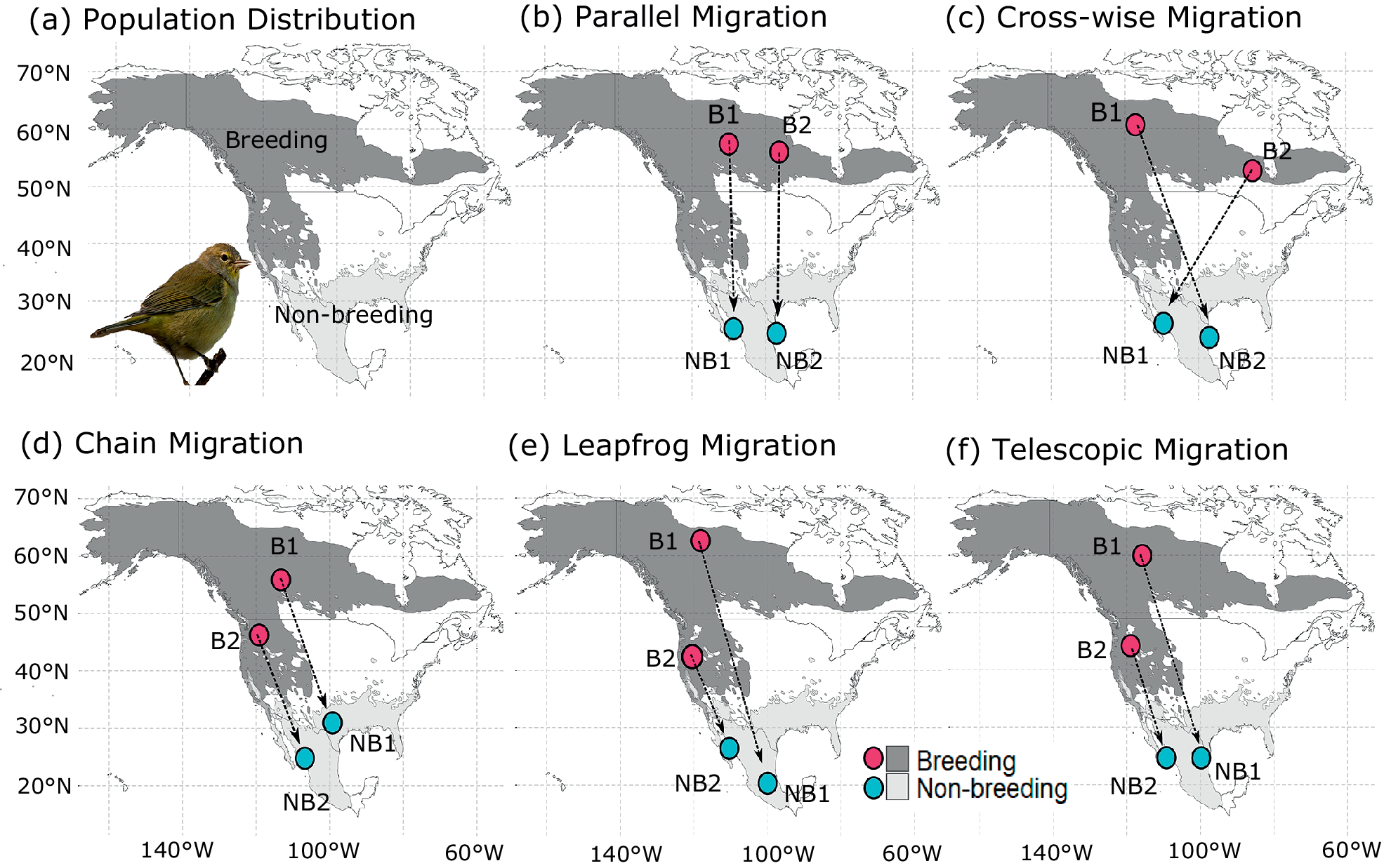
Figure 1. Long description
A multi-panel set of six maps of North America with a latitude and longitude grid.
* Panel a, Population Distribution. Shows a dark grey breeding range across Canada, Alaska, and the Western United States, and a light grey non-breeding range in the Southern United States and Mexico. A photo of an Orange-crowned Warbler is in the bottom left.
* Panel b, Parallel Migration. Two pink dots labeled B 1 and B 2 are in the North. Dotted arrows point vertically South to two blue dots labeled N B 1 and N B 2. B 1 moves to N B 1 and B 2 moves to N B 2 without crossing.
* Panel c, Cross-wise Migration. B 1 is in the Northwest and B 2 is in the Northeast. Dotted arrows cross each other, pointing B 1 to N B 2 in the Southeast and B 2 to N B 1 in the Southwest.
* Panel d, Chain Migration. B 1 is in the North and B 2 is further South. Dotted arrows show B 1 moving to N B 1 in the North of the wintering range, while B 2 moves to N B 2 in the South of the wintering range.
* Panel e, Leapfrog Migration. B 1 is in the far North and B 2 is further South. Dotted arrows show B 1 flying over B 2 to reach the southernmost wintering area N B 1, while B 2 moves to the northernmost wintering area N B 2.
* Panel f, Telescopic Migration. B 1 is in the North and B 2 is in the South. Dotted arrows show both populations converging toward the same latitude in the non-breeding range at N B 1 and N B 2.
Nevertheless, interpreting isotopic patterns correctly requires careful consideration of the species’ ecology. For the Orange-crowned Warbler, latitudinal sex segregation (Komar et al. Reference Komar, O’Shea, Peterson and Navarro-Sigüenza2005) and age-related isotopic offsets (Langin et al. Reference Langin, Reudink, Marra, Norris, Kyser and Ratcliffe2007) could potentially confound connectivity estimates. Furthermore, Orange-crowned Warblers during the non-breeding season occupy a vast range of habitats, from sea-level thorn-scrub to high-elevation montane pine-oak forests (Gilbert et al. Reference Gilbert, Sogge, Van Riper and Rodewald2020). Winter site fidelity in this species appears to be relatively low and habitat-dependent (Conway and Brush Reference Conway and Brush2018), and several parulids are known to segregate across elevational gradients or distinct ecoregions during the stationary period (Barçante et al. Reference Barçante, Vale and Alves2017).
To identify which demographic trajectories of Orange-crowned Warbler breeding populations are associated with specific non-breeding sites in Mexico, we developed a framework that integrates migratory connectivity patterns with long-term trends of relative abundance. Our framework identifies geographic breeding origins of individuals sampled at multiple non-breeding sites to determine whether particular regions in Mexico disproportionately host individuals from declining breeding populations. Our workflow begins with feather sampling along a large-scale transect across western, central, and eastern Mexico during non-breeding months. We then process feathers for stable hydrogen isotope analysis to infer proportions of geographic origins. We use migratory connectivity metrics to determine whether Orange-crowned Warblers exhibit one or more of the following five migration strategies: (1) parallel migration, in which individuals from western and eastern breeding populations migrate along longitudinal routes to wintering sites; (2) crosswise migration, whereby breeding populations from opposite ends of the breeding range cross paths en route to their respective wintering areas; (3) chain migration, in which southern breeders winter closer to their breeding sites compared to more northerly populations; (4) leapfrog migration, in which northern breeders do not stop at wintering areas used by southern breeders and move further south; or (5) telescopic migration, in which populations breeding at different latitudes winter at a similar latitude (Figure 1). These movement scenarios yield distinct predictions for spatial isotopic patterns and migratory connectivity metrics across non-breeding sites. Additionally, this framework offers insights into the selective pressures shaping migration and guides population-specific conservation actions.
Although stable isotopes have been widely used to infer seasonal movements in migratory species, our study addresses a key gap in understanding migratory connectivity, specifically how birds from different breeding populations and with different demographic trajectories mix in shared non-breeding areas. Using the Orange-crowned Warbler as a case study, we show the importance of data integration for quantifying population-specific connectivity to inform effective conservation planning.
Methods
Sampling sites
We analysed Orange-crowned Warbler feather samples across nine non-breeding sites in Mexico (Table 1). We categorised these sites as northern and southern based on the Tropic of Cancer (~23°26’ N), distinguishing subtropical from tropical wintering ecoregions (Figure 2). We defined a northern group above ~23°26′ N (TAMQ, CABA, PICH, and PATO) and a southern group below ~23°26′ N (ACPF, ESJC, FLOR, ROCA, and ARCO; Table 1). Additionally, we classified sampling sites as being part of a Pacific or Gulf group based on their position relative to the Sierra Madre Occidental (Table 1).
Orange-crowned Warbler feather-sampling sites in Mexico. For each site, the table provides the location name, unique site identifier (Site ID), geographic coordinates (latitude and longitude), elevation in metres above sea level (m.a.s.l.), habitat type, and the corresponding Level II ecoregion. Sampling details include the years of data collection, the total number of feather samples collected, and the Mexican state where the site is located. We divided the sampling sites into a northern group (above the Tropic of Cancer ~23°26′ N) and a southern group (below the Tropic of Cancer ~23°26′ N). We classified sites west of the Sierra Madre Occidental as the Pacific group and those east of the Sierra Madre Occidental as the Gulf group.

Table 1. Long description
The table contains 12 columns: Site, Site I D, Latitude, Longitude, Elevation in m dot a dot s dot l dot, Habitat Type, Eco-regions, Years, Samples, State, Tropic of Cancer ~23 degrees 26 minutes North, and Sierra Madre Occidental.
* Roca volcanica y cañada (ROCA): 19.2511, -99.1979, 2248.92 m, High-elevation pine-oak forest, Transversal Neo-Volcanic System, 2013, 56 samples, Mexico City, Southern, Gulf.
* La Flor del Desierto (FLOR): 19.6155, -103.6200, 1378.12 m, Tropical dry forest and deciduous shrubland, Transversal Neo-Volcanic System, 2007-2008, 29 samples, Jalisco, Southern, Pacific.
* Parque Estatal Sierra de Tepotzotlan (ARCO): 19.7500, -99.3042, 2276.54 m, Subtropical thorn-forest and riparian woodland, Transversal Neo-Volcanic System, 2005-2009, 32 samples, Estado de México, Southern, Gulf.
* Alta Cima Primary Forest (ACPF): 23.0553, -99.1853, 372.41 m, Tamaulipan semiarid thorn-scrub, Eastern Sierra Madre, 2006-2010, 15 samples, Tamaulipas, Southern, Gulf.
* Estero de San José del Cabo (ESJC): 23.0833, -109.667, 14.05 m, Arid tropical scrub and palm groves, Sierra and Plains of El Cabo, 1997, 22 samples, Baja California Sur, Southern, Pacific.
* Tamaulipas (TAMQ): 23.9441, -99.0974, 355.22 m, Tamaulipan semiarid thorn-scrub, Tamaulipas-Texas Semiarid Plain, 2008, 8 samples, Tamaulipas, Northern, Gulf.
* Cabañas La Muralla (CABA): 24.0878, -104.9310, 2453.67 m, Highland pine-oak forest, Western Sierra Madre, 2018, 3 samples, Durango, Northern, Pacific.
* Pichihuila (PICH): 24.4275, -107.4310, 169.51 m, Subtropical deciduous forest, Western Pacific Coastal Plain, 2003-2009, 11 samples, Sinaloa, Northern, Pacific.
* Patolandia (PATO): 25.0261, -107.987, 3.42 m, Coastal subtropical thorn-scrub and mangroves, Western Pacific Coastal Plain, 2003, 13 samples, Sinaloa, Northern, Pacific.
Ecoregions at the non-breeding grounds where Orange-crowned Warblers were sampled. Red dots show the capture sites across Mexico.
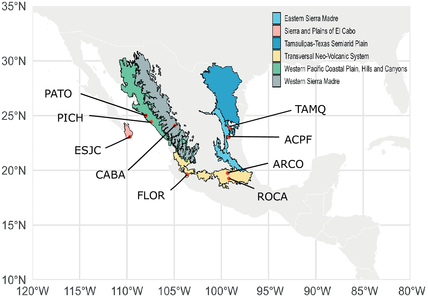
Figure 2. Long description
A map of Mexico and surrounding regions with a latitude and longitude grid.
Legend in the Northeast:
* Light blue: Eastern Sierra Madre.
* Pink: Sierra and Plains of El Cabo.
* Dark blue: Tamaulipas-Texas Semiarid Plain.
* Yellow: Transversal Neo-Volcanic System.
* Green: Western Pacific Coastal Plain, Hills and Canyons.
* Gray: Western Sierra Madre.
Sampling Sites and Ecoregions from Northwest to Southeast:
* E S J C: Located in the pink Sierra and Plains of El Cabo ecoregion on the southern tip of Baja California.
* P A T O and P I C H: Located in the green Western Pacific Coastal Plain ecoregion along the Northwest coast.
* C A B A: Located in the gray Western Sierra Madre ecoregion inland from the Northwest coast.
* T A M Q and A C P F: Located in the dark blue Tamaulipas-Texas Semiarid Plain ecoregion in the Northeast.
* F L O R, A R C O, and R O C A: Located in the yellow Transversal Neo-Volcanic System ecoregion stretching across Central Mexico.
The light blue Eastern Sierra Madre ecoregion is situated in the East-Central part of the country, adjacent to the dark blue and yellow regions.
Feather sampling
We collected a total of 189 feather samples under Mexican federal permits (SGPA/DGVS/00685/08; SGPA/DGVS/07644/10) through the Monitoreo de Sobrevivencia Invernal (MoSI; Monitoring Overwinter Survival) programme, an international network of standardised bird-banding stations coordinated by the Institute for Bird Populations (IBP) (DeSante et al. Reference DeSante, Sillett, Siegel, Saracco, Romo de Vivar Alvarez, Morales, Ralph and Rich2005). The MoSI capture protocols followed a standardised mist-netting design across all stations, with birds captured using mist nets operated under a consistent sampling protocol and without the use of audio playback (DeSante et al. Reference DeSante, Sillett, Siegel, Saracco, Romo de Vivar Alvarez, Morales, Ralph and Rich2005). Bird extraction, handling, banding, and feather sampling adhered to established ethical and animal welfare guidelines (North American Banding Council 2001; Fair et al. Reference Fair, Paul, Jones and Bies2023). The feathers were archived at the Center for Tropical Research (University of California, Los Angeles).
Stable isotope analysis
We prepared tail feathers for stable hydrogen isotope (δ²H) analysis using a standard washing protocol (Paritte and Kelly Reference Paritte and Kelly2009; Chew et al. Reference Chew, Kelly and Contina2019). To remove debris and oil contaminants, we cleaned feathers with a 2:1 chloroform:methanol solution for 30 seconds, dried them overnight at room temperature, and then rinsed each feather with a dilute detergent solution (1:30 Fisher Scientific Versa-Clean: DI water). Then, we cut a subsample from the distal end of each feather and weighed it to 200 ± 10 μg using a Mettler Toledo microbalance (model XS3DU), and placed it into 3.5 mm × 5 mm silver capsules (Costech 041066).
Before analysis, we equilibrated the samples and standards for at least three weeks to the local laboratory environment (Wassenaar and Hobson Reference Wassenaar and Hobson2003) at the Environmental Stable Isotope Laboratory, University of Oklahoma, Norman, OK, USA. We performed stable hydrogen isotope measurements using a ThermoFinnigan Delta V isotope ratio mass spectrometer coupled to a Thermal Conversion Elemental Analyzer (Thermo Scientific). We expressed stable hydrogen isotope ratios in delta notation (δ²H) as parts per thousand (‰) relative to the Vienna Standard Mean Ocean Water (VSMOW) according to the formula: δ²Hsample = [(Rsample/Rstandard) − 1] x 1000. We used the Caribou Hoof Standard (n = 32; δ²H CBS = −157.0‰), Kudu Horn Standard (n = 34; δ²H KHS = −35.3‰), and Brown-headed Cowbird feathers (n = 34; δ²H BHCO = −42.7‰) to calibrate δ²H values measured in feather samples. We used the standard deviations (SDs) of the reference materials to express analytical precision: BHCO (n = 34; SD = 2.2), KHS (n = 34; SD = 1.2), and CBS (n = 32; SD = 1.3). We analysed three reference standards for every eight samples during all mass spectrometer runs.
Calibration and geographical assignments
We implemented a Bayesian analytical framework using the R package assignR to reconstruct the breeding areas of the Orange-crowned Warbler (Ma et al. Reference Ma, Vander Zanden, Wunder and Bowen2020). First, we rescaled stable hydrogen isotope values in precipitation (δ²Hp) from a North American geostatistical model (Bowen et al. Reference Bowen, Wassenaar and Hobson2005) to known-origin samples provided by Hobson et al. (Reference Hobson, Van Wilgenburg, Wassenaar and Larson2012) and Hobson and Koehler (Reference Hobson and Koehler2015) using the calRaster function in assignR (Ma et al. Reference Ma, Vander Zanden, Wunder and Bowen2020). Although species-specific calibration provides the highest accuracy, it requires tissues from known-origin individuals. Since known-origin data for our target species were unavailable, we used calibration data from a closely related species (Hobson et al. Reference Hobson, Van Wilgenburg, Wassenaar and Larson2012; Contina et al. Reference Contina, Magozzi, Vander Zanden, Bowen and Wunder2022a). Our Orange-crowned Warbler dataset consisted entirely of unknown-origin feathers (Table S2). For calibration, we used 22 Northern Yellow Warblers Setophaga aestiva feathers from 10 known moulting sites, a species with a similar size, diet, and spatial distribution (Hobson et al. Reference Hobson, Van Wilgenburg, Wassenaar and Larson2012).
To infer the origin of birds sampled in Mexico, we generated individual-based posterior probability density maps restricted to the breeding breeding range of the Orange-crowned Warbler (BirdLife International and Handbook of the Birds of the World 2021) using the pdRaster function in assignR (Ma et al. Reference Ma, Vander Zanden, Wunder and Bowen2020).
Clustering and regional assignment
We used the R package isocat (Isotope Origin Clustering and Assignment Tools) to identify potential geographic clusters of origin (Campbell Reference Campbell2020). We constructed a similarity matrix using the function simmatrixMaker based on individual assignment probabilities. Then, we performed hierarchical clustering using the function clusterSimmatrix, employing correlation-based distance metrics and 1,000 bootstrap replicates to assess the robustness of the clustering. We determined the clusters by cutting the dendrogram at a predefined height (h = 0.5). We chose this height to balance cluster differentiation with biological relevance using the cutree function from the dendextend R package (Galili Reference Galili2015). We calculated the mean assignment probability surfaces for each cluster using the meanAggregateClusterProbability function, which aggregates posterior probability surfaces across individuals within a cluster. We visualised these mean surfaces in geographic space to assess potential differences in spatial origin among the clusters.
Migratory connectivity analysis
We used the R package MigConnectivity (Cohen et al. Reference Cohen, Hostetler, Hallworth, Rushing, Sillett and Marra2018; Hostetler et al. Reference Hostetler, Cohen, Bossu, Scarpignato, Ruegg and Contina2025) to quantify the strength of migratory connectivity in Orange-crowned Warblers, using a combination of isotope assignment data, abundance estimates, and regional classification across both the breeding and non-breeding ranges. We generated probable breeding origin assignment rasters using stable isotope analysis of feather samples, with centroids representing the most probable breeding origin locations for individual birds. We defined non-breeding origin regions by intersecting the Orange-crowned Warbler’s non-breeding range polygon derived from species distribution data with Level II North American ecoregions (https://www.epa.gov/eco-research/ecoregions-north-america). We retained only ecoregions containing at least one site where we captured the birds. We retained Eastern Sierra Madre, Sierra and Plains of El Cabo, Tamaulipas-Texas Semiarid Plain, Transversal Neo-Volcanic System, Western Pacific Coastal Plain Hills and Canyons, and Western Sierra Madre as the ecoregions where birds were captured (Figure 2). For connectivity analysis, we defined these origin sites as distinct population regions (Hostetler et al. Reference Hostetler, Cohen, Bossu, Scarpignato, Ruegg and Contina2025).
We used eBird Status and Trends data (2022) to obtain weekly relative abundance layers at a 3 km spatial resolution (Fink et al. Reference Fink, Auer, Johnston, Strimas-Mackey, Ligocki and Robinson2023). We defined the breeding and non-breeding periods by extracting the abundance data from the specific temporal windows that the eBird Status and Trends models define as the peak of each season (Fink et al. Reference Fink, Auer, Johnston, Strimas-Mackey, Ligocki and Robinson2023). Breeding weeks spanned from 21 June to 12 July, when the species is on territory, and the non-breeding weeks spanned from 6 December to 1 February, when the species is stationary on its wintering grounds. This approach aligns with the species-specific seasonal definitions established within the eBird Status and Trends framework, thereby avoiding the inclusion of individual data during migratory periods. We extracted and averaged the weekly raster values for each breeding and non-breeding site polygon and computed normalised abundance across time and space. We used the weekly average because it provides a more reliable measure of typical abundance than the weekly maximum, which can be heavily influenced by short-term random events or extreme values. We used these values as priors for connectivity modelling and as a proxy for regional population density.
To estimate migratory transition probabilities, we used the estTransition function in the MigConnectivity package (Hostetler et al. Reference Hostetler, Cohen, Bossu, Scarpignato, Ruegg and Contina2025). Each individual was treated as originating from a known non-breeding location and assigned a probability surface (raster) representing its likely breeding location. We computed the transitions between non-breeding (origin) and breeding (target) sites using a Bayesian framework that incorporates both spatial uncertainty and prior abundance estimates. The resulting matrix (ψ) reflects the estimated probability that birds from a given breeding site migrated to a specific non-breeding site.
We estimated the overall strength of migratory connectivity (MC) using the estStrength function, which calculates the correlation between spatial distances among origin and target site centroids and the migratory transition probabilities (Roberts et al. Reference Roberts, Scarpignato, Huysman, Hostetler and Cohen2023; Hostetler et al. Reference Hostetler, Cohen, Bossu, Scarpignato, Ruegg and Contina2025). This method quantifies the extent to which migratory movements are geographically structured. We used 5,000 simulation replicates to assess the robustness of estimates, incorporating uncertainty in both spatial and probabilistic assignment data.
Demographic and environmental drivers of population variation
To evaluate demographic segregation across the non-breeding range, we implemented a two-tailed Fisher’s exact test (Mundry and Fischer Reference Mundry and Fischer1998) and constructed a linear model to test the effects of site and sex and to determine whether sexes within the same non-breeding site originated from different breeding regions: δ²H ~ Site + Sex + Site × Sex. Prior to modelling, we retained sampling sites only if each site provided at least three individuals of each sex. We removed sites that had fewer than six samples (CABA) and individuals of unknown sex (ACPF). To address within-site variation while accounting for unequal sample sizes across groups, we implemented an analysis of variance (ANOVA) (Shaw and Mitchell-Olds Reference Shaw and Mitchell-Olds1993). We used the car package (Fox and Weisberg Reference Fox and Weisberg2019) and evaluated the main effects independently of the order of entry in the presence of the interaction.
We incorporated the Site × Sex interaction to test the hypothesis that the relationship between sex and geographic origin varies across non-breeding capture sites. To evaluate sex-based differences within specific sites, we derived estimated marginal means (EMMs) (Searle et al. Reference Searle, Speed and Milliken1980) from the full interactive model. We evaluated the demographic composition of our dataset by categorising age groups into adults (after-hatch-year = AHY, n = 106; second-year = SY, n = 26) and young (hatch-year = HY, n = 4). We then modelled the effects of site and age group on feather isotope values (δ²H ~ Site + Age Group).
To assess potential habitat-driven segregation across elevational gradients, we extracted the elevation in metres above sea level (m.a.s.l.) of each sampling site using the Shuttle Radar Topography Mission (SRTM) Digital Elevation Model (Farr et al. Reference Farr, Rosen, Caro, Crippen, Duren and Hensley2007), which ranged from coastal lowlands (10 m.a.s.l.) to highland pine–oak forests (2,450 m.a.s.l.). We then used a Spearman rank correlation to test for relationships between site elevation and feather δ²H values. This analysis allowed us to determine whether birds from different breeding populations occupied different elevational zones during the non-breeding season, a behaviour observed in other wintering warblers (Barçante et al. Reference Barçante, Vale and Alves2017).
Orange-crowned Warbler breeding population variation over time
We obtained the North American Breeding Bird Survey (BBS) dataset using the bbsBayes2 R package (Edwards et al. Reference Edwards, Smith and LaZerte2026). The BBS is a long-term, standardised monitoring programme that began in 1966 and continues today across the United States, Canada, and Mexico (Sauer et al. Reference Sauer, Pardieck, Ziolkowski, Smith, Hudson and Rodriguez2017). Each survey route is 39.4 km long, with 50 stops spaced at 0.8 km intervals. At each stop, observers count all birds seen or heard during a three-minute period. We used the cluster polygons derived from stable isotope data to define spatial regions within the breeding range of the Orange-crowned Warbler. We aggregated Breeding Bird Survey (BBS) data within these clusters to estimate abundance trends over time. We retrieved data on Orange-crowned Warbler occurrences across all available routes in Canada and the United States using the fetch_bbs_data function. We used both the United States Geological Survey (USGS) and the Canadian Wildlife Service (CWS) stratifications, which are based on the intersection of political boundaries and Bird Conservation Regions, as provided in Ziolkowski et al. (Reference Ziolkowski, Lutmerding, English and Hudson2024).
GAMYE model specification
We modelled population trajectories using the Generalised Additive Model with Year Effects (GAMYE) framework, implemented in bbsBayes2 (Smith and Edwards Reference Smith and Edwards2020; Smith et al. Reference Smith, Aponte, Binley, Cox, Daly and Donkersteeg2024a; Smith et al. Reference Smith, Binley, Daly, Edwards, Ethier and Frei2024b; Ziolkowski et al. Reference Ziolkowski, Lutmerding, English and Hudson2024; Edwards et al. Reference Edwards, Smith and LaZerte2026). This hierarchical Bayesian model links the observed counts to predictors via a log link and assumes a Poisson distribution for the raw count data. It accounts for observer effects, sampling error, and annual fluctuations while describing long-term trends using smooth functions (Link et al. Reference Link, Sauer and Niven2020; Edwards et al. Reference Edwards, Smith and LaZerte2026). We ran the models using the default MCMC settings of four chains, each with 1,000 warmup iterations and 1,000 sampling iterations, yielding 4,000 posterior samples for analysis.
We generated annual relative abundance indices for each stratification at the stratum level using the generate_indices function. For each year, we extracted the posterior mean and 95% credible intervals. To reduce potential bias from stratification choice, we averaged the corresponding CWS and USGS indices by stratum and year. This produced a unified set of relative abundance indices. To examine population dynamics at ecologically meaningful spatial units, we linked BBS strata to the probability of origin cluster polygons that we previously delineated from the feather isotope analysis. We calculated cluster-level relative abundance trajectories by averaging indices across all strata within each cluster. For each cluster and year, we derived the mean relative abundance and propagated uncertainty by averaging the lower and upper 95% credible bounds.
Results
Cluster assignments
Analysis of feather isotope data from 189 individuals revealed six distinct breeding origin clusters across North America (Figures 3 and 4; maps for each individual appear in Supplementary material). These clusters correspond to broad geographic regions across North America, spanning from the high Arctic tundra of northern Alaska and Canada (Cluster 1) and the northern and interior boreal forests (Clusters 2, 3, and 4) to the temperate rainforests and mountains of the Pacific Northwest and coastal southwest Alaska (Clusters 5 and 6).
Representative posterior probability density maps for six individual Orange-crowned Warblers sampled on the non-breeding grounds (red dots). These individuals were selected as examples to illustrate the range of feather δ²H values observed in our dataset (approximately from −149‰ to −58‰) and the corresponding variation in inferred breeding origins across the North American latitudinal stable isotope gradient. Bright yellow indicates areas with the highest posterior probability of breeding and moult origin based on stable isotope assignments. The complete set of individual assignment maps is provided in the Supplementary Material.
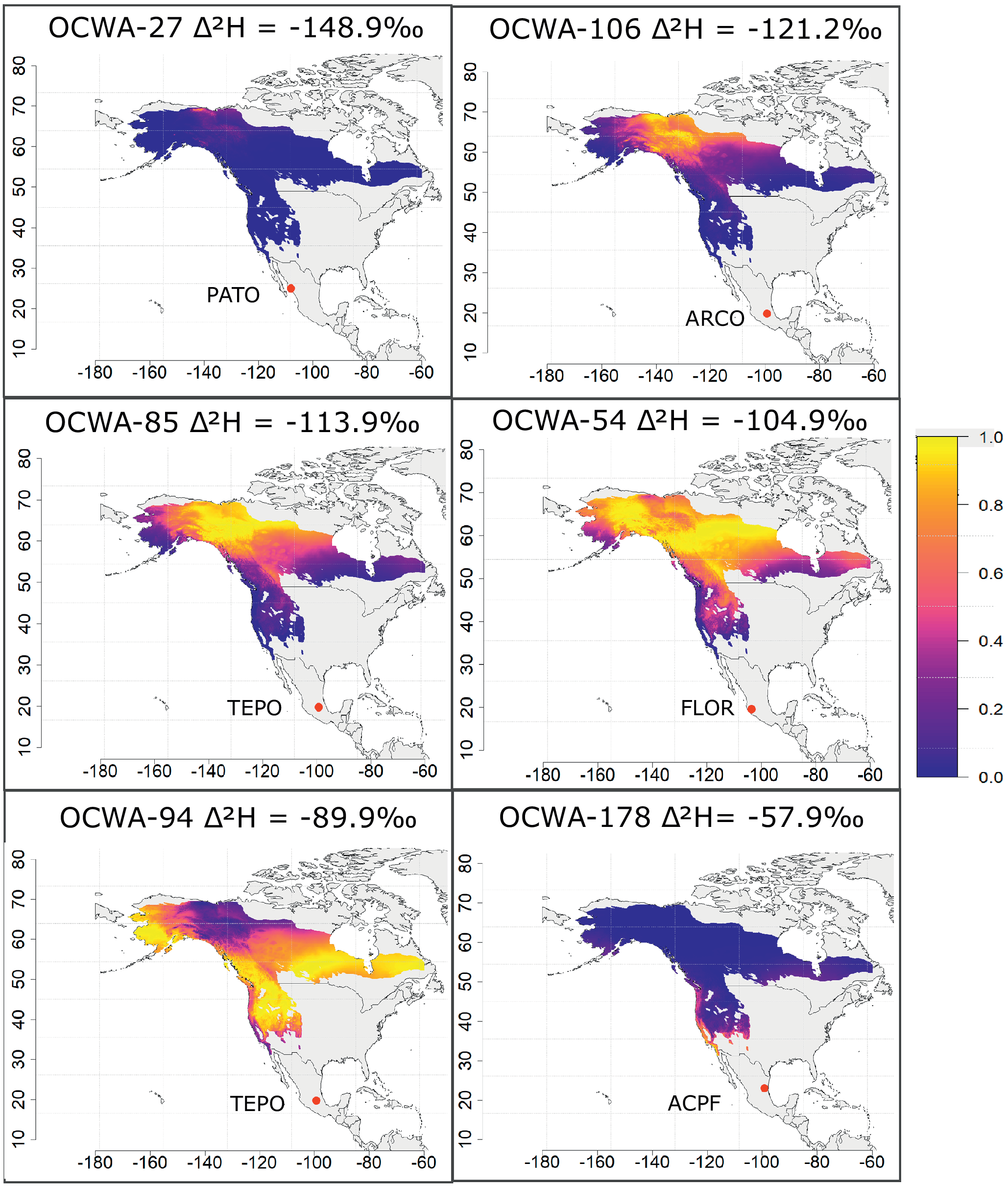
Figure 3. Long description
A six-panel series of North American maps, each with a latitude y-axis from 10 to 80 and a longitude x-axis from -180 to -60. A color scale on the right indicates probability from 0.0 (dark blue) to 1.0 (bright yellow).
* Top-Left: O C W A dash 27, delta super 2 H equals minus 148.9 per mille. High probability (yellow) is concentrated in the far Northwest, specifically Alaska and Northwest Canada. A red dot is at P A T O in Mexico.
* Top-Right: O C W A dash 106, delta super 2 H equals minus 121.2 per mille. High probability shifts Southeast from Alaska into Central Canada.
* Middle-Left: O C W A dash 85, delta super 2 H equals minus 113.9 per mille. High probability covers a broad band across Central Canada and the Northern United States. A red dot is at T E P O in Mexico.
* Middle-Right: O C W A dash 54, delta super 2 H equals minus 104.9 per mille. High probability is centered in the North-Central United States and Southern Canada. A red dot is at F L O R in Mexico.
* Bottom-Left: O C W A dash 94, delta super 2 H equals minus 89.9 per mille. High probability is concentrated in the Western United States and Southwestern Canada. A red dot is at T E P O in Mexico.
* Bottom-Right: O C W A dash 178, delta super 2 H equals minus 57.9 per mille. High probability is restricted to the Southwestern United States and Pacific Coast. A red dot is at A C P F in Mexico.
The probability of origin clusters of Orange-crowned Warblers based on δ²H values in feathers sampled during the non-breeding season across nine sites in Mexico. Coloured polygons on the map show the cluster of origin derived from stable isotope analysis. Each pie chart shows the proportion of breeding individuals sampled at non-breeding sites.
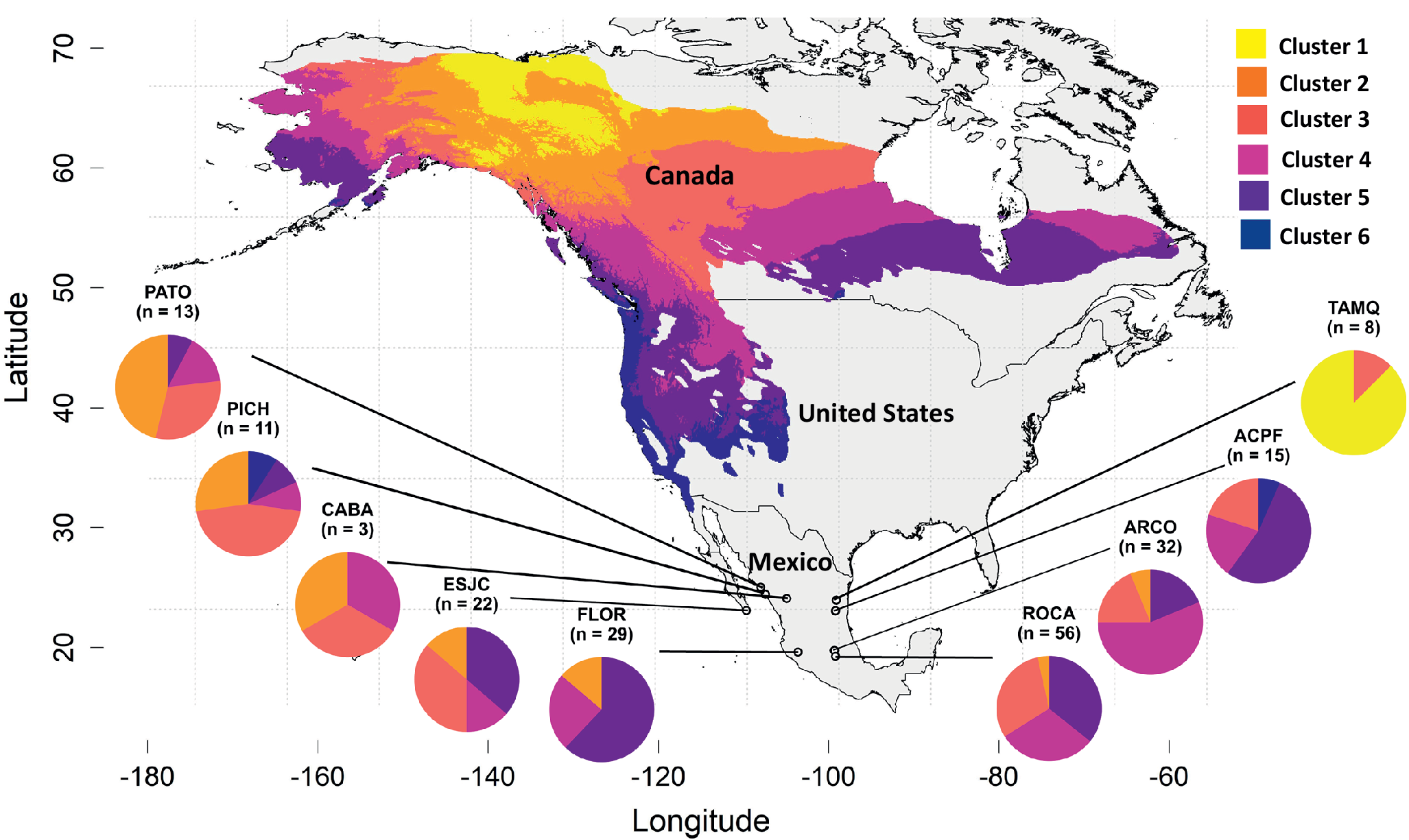
Figure 4. Long description
A geographical map of North America with Latitude on the Y axis from 20 to 70 and Longitude on the X axis from negative 180 to negative 60.
Six colored polygons represent breeding origin clusters.
* Cluster 1 (yellow) is in Northern Canada and Alaska.
* Cluster 2 (orange) is in Central Canada.
* Cluster 3 (red) is in Southern Canada and the Northern United States.
* Cluster 4 (pink) spans the Central United States.
* Cluster 5 (purple) covers the Southern United States and Western coast.
* Cluster 6 (dark blue) is concentrated in the Southwestern United States and Northern Mexico.
Nine pie charts are connected by lines to specific sampling sites in Mexico. From West to East, they are.
* P A T O (n equals 13) mostly orange and pink.
* P I C H (n equals 11) mostly orange and red.
* C A B A (n equals 3) equal parts orange, red, and pink.
* E S J C (n equals 22) mostly orange, pink, and purple.
* F L O R (n equals 29) mostly purple and pink.
* R O C A (n equals 56) mostly pink and purple.
* A R C O (n equals 32) mostly purple and pink.
* A C P F (n equals 15) mostly purple and pink.
* T A M Q (n equals 8) mostly yellow with a small red slice.
Most wintering sites hosted individuals from three to five distinct breeding clusters, indicating a high degree of population mixing (Figure 4). For example, the PICH site hosted individuals from five distinct clusters, while ESJC and PATO each hosted birds from four clusters. A notable exception to this pattern was observed in the easternmost Mexican site, TAMQ, where 87% of individuals originated from a single breeding population, Cluster 1. The composition of these mixed-origin groups suggests a distinct east-west geographic pattern across the wintering grounds (Figure 4). Western sites were primarily composed of individuals from Clusters 2 and 3, while eastern sites were characterised by a higher proportion of birds from northern breeding populations (Clusters 1 and 4).
Migratory connectivity
We found a high transition probability (ψ = 0.80) between the northernmost breeding population (Cluster 1) and the easternmost non-breeding site, the Tamaulipas-Texas Semiarid Plain (Figure 5; Supplementary material Table S1). In contrast, most other breeding populations showed only weak to negligible transition probabilities (ψ < 0.25) to this and other ecoregions (see Supplementary material Table S1 for all transition probabilities). We did, however, observe moderate transition probabilities (ψ = 0.26–0.40) for some central and western breeding populations (Clusters 1 and 2) with wintering grounds in the Western Sierra Madre and the Western Pacific Coastal Plain. Taken together, and aside from some exceptions (i.e., Cluster 1), the transition matrix revealed a migratory system characterised by a broader pattern of weak connectivity. Reflecting these patterns, the overall strength of migratory connectivity for the species was weak (MC = 0.18, SE = 0.05), indicating that breeding populations are broadly distributed across the non-breeding range.
Mean transition probabilities (ψ) of Orange-crowned Warbler probable breeding clusters to non-breeding ecoregions. The matrix shows a migratory system characterised by one strong connection within a broader pattern of weak connectivity. We found a high transition probability (ψ = 0.80) between the northernmost breeding population (Cluster 1) and the easternmost non-breeding ecoregion, the Tamaulipas-Texas Semiarid Plain (TTSP). In contrast, other transition probabilities were weak (ψ < 0.25), with some moderate transitions (ψ = 0.26–0.40) observed for central and western breeding populations (e.g., Clusters 1 and 2) to the Western Sierra Madre (WSM) and Western Pacific Coastal Plain (WPCPHC). Non-breeding ecoregions are abbreviated as: SPEC (Sierra and Plains of El Cabo), WPCPHC (Western Pacific Coastal Plain Hills and Canyons), WSM (Western Sierra Madre), TNVS (Transversal Neo-Volcanic System), ESM (Eastern Sierra Madre), and TTSP (Tamaulipas-Texas Semiarid Plain).

Figure 5. Long description
The y-axis represents Mean Transition Probability (Psi) ranging from 0.00 to 0.75. The x-axis lists six eco-regions: S P E C, W P C P H C, W S M, T N V S, E S M, and T T S P. A legend on the right identifies six breeding clusters by color: Cluster 1 (yellow), Cluster 2 (orange), Cluster 3 (light red), Cluster 4 (dark pink), Cluster 5 (purple), and Cluster 6 (dark blue).
Data distribution by eco-region:
* S P E C: All clusters show low probabilities between 0.05 and 0.25.
* W P C P H C: Cluster 1 and Cluster 2 show moderate probabilities around 0.30 to 0.40, while others are below 0.15.
* W S M: Clusters 1, 2, and 3 show moderate probabilities between 0.20 and 0.35 with large error bars; others are low.
* T N V S: All clusters are tightly grouped with low probabilities between 0.05 and 0.25.
* E S M: Probabilities show a slight upward trend from Cluster 1 to Cluster 5, peaking around 0.25.
* T T S P: Cluster 1 shows a distinct high peak at 0.80. Cluster 2 is low at approximately 0.18, and Clusters 3 through 6 are near 0.00.
Demographic and environmental variation among populations
The two-tailed Fisher’s exact test on the known-sex subset (n = 128) showed no sex differences (P = 0.540) between northern (16 males, 16 females) and southern birds (41 males, 55 females). Similarly, age classes were evenly distributed across broad latitudinal regions (P = 0.630). Additionally, sex had no effect on isotope values (P = 0.303).
When testing within-site variation, our linear model showed an effect of site on feather isotope values (P < 0.001) but no effect of sex (P = 0.498). The Site × Sex interaction was not significant (P = 0.781), showing that isotopic values and geographic breeding origins did not differ between males and females within non-breeding sites. Modelling the effects of site and age group on feather isotope values showed no effect of age group (P = 0.118).
While our non-breeding sampling spanned a wide elevational gradient from coastal mangroves (20 m.a.s.l.) to highland pine-oak forests (2,400 m.a.s.l.), we found no correlation between site elevation and isotopic values indicative of latitudinal breeding origin (ρ = 0.139, P = 0.057). This suggests that breeding populations are mixing across the vertical landscape of Mexico and that the weak connectivity we observed is a consistent pattern across different habitat types.
Orange-crowned Warbler breeding population trajectories
The breeding clusters exhibited distinct long-term population trajectories from 1966 to 2023 (Figure 6). Clusters 1, 3, and 4 showed similar patterns, with populations generally increasing until peaking between approximately 2000 and 2010 before entering a period of decline. In contrast, populations in the Pacific Northwest and coastal regions showed long-term declines. Specifically, Cluster 6 experienced the most pronounced decline, losing approximately two-thirds of its relative abundance over the 57-year period. The remaining populations were comparatively stable. For example, Cluster 2 exhibited a slight increase until approximately 1990, after which its population trajectory remained relatively stable with minor fluctuations, while Cluster 5 maintained its stability throughout the entire period.
Annual population trajectory of Orange-crowned Warbler from 1966 to 2023 calculated from Breeding Bird Survey data relative to spatial clusters of probability of origin inferred from stable isotope data. The solid line represents the estimated trajectory of relative abundance, and the shaded area indicates 95% credible intervals. Clusters 3 and 4 increased until the year 2000, then declined; Cluster 2 declined from the 1970s, with minor fluctuations after the year 2000; Cluster 5 remained relatively stable; Cluster 6 showed a long-term decline to approximately one-third of its initial levels. Cluster 1 showed a decline in the last decade.

Figure 6. Long description
A six-panel line graph layout labeled a through f. Each panel features a y-axis for Relative Abundance and an x-axis for Year. A solid black line tracks the estimated trajectory, surrounded by a light blue shaded area representing the 95 percent credible intervals.
* Panel a Cluster 1. The x-axis spans 1982 to 2022. The line shows a steady increase from an abundance of 3 to a peak of 15 around 2010, followed by a sharp decline to approximately 7 by 2022. The inset map highlights a northern region in purple.
* Panel b Cluster 2. The x-axis spans 1966 to 2023. The line starts at 10, rises gradually to nearly 20 by 2010, and then slightly declines. The shaded interval is extremely wide in the early years. The inset map highlights a large northwestern area.
* Panel c Cluster 3. The line shows a bell-shaped curve, rising from 3.5 in 1966 to a peak of 9 in the late 1990s, then steadily declining to 4 by 2023. The inset map highlights a central-northern band.
* Panel d Cluster 4. Similar to Cluster 3, the line rises from 1.5 to a peak of 3.5 in the late 1990s before declining back toward 2. The inset map highlights northeastern regions.
* Panel e Cluster 5. The line remains relatively flat, fluctuating between 2.5 and 3.5 across the entire time series. The inset map highlights western and central regions.
* Panel f Cluster 6. The line shows a significant long-term decline, starting at an abundance of 10 in 1966 and dropping to approximately 4 by 2023. The inset map highlights the Pacific coast region.
Discussion
Our study integrated stable isotope analysis with long-term population data to reveal three key aspects of the Orange-crowned Warbler’s annual cycle. First, we found that this species exhibits predominantly weak migratory connectivity, with most non-breeding sites hosting individuals from multiple breeding origins. This reinforces evidence that low migratory connectivity and high population mixing are typical of long-distance migrants (Finch et al. Reference Finch, Butler, Franco and Cresswell2017). Second, we found that birds migrating to Mexico originate from at least six distinct breeding clusters. Third, analysis of Breeding Bird Survey data revealed divergent demographic trajectories among these six breeding clusters, including both stable and declining populations. The contrasting demographic patterns suggest that both breeding and non-breeding factors may drive regional population declines. These differences matter because, when populations with non-uniform demographic trends overlap at the non-breeding grounds, local declines could be masked (Palacio et al. Reference Palacio, Abarca, Armenteras, Balza, Dollar and Froese2023). Additionally, degradation of non-breeding sites could negatively impact breeding individuals from different regions, underscoring the conservation importance of non-breeding habitats and carry-over effects across seasons (Lambert and Hannon Reference Lambert and Hannon2000; Webster and Marra Reference Webster, Marra, Greenberg and Marra2005; Norris and Marra Reference Norris and Marra2007; McKinnon et al. Reference McKinnon, Stanley and Stutchbury2015; Dossman et al. Reference Dossman, Matthews and Rodewald2017; Cooper et al. Reference Cooper, Yanco, Rushing, Sillett and Marra2024).
The broad distribution of our nine non-breeding sampling sites across Mexico provided a framework for evaluating population-level migration strategies. Across these sites, the most common pattern we observed was telescopic migration, in which different breeding populations converge at similar latitudes during the non-breeding season, as indicated by the widespread occurrence of multiple clusters within single wintering sites. This pattern was evident in the mixing of individuals from our six breeding clusters occurring in the Pacific and Gulf groups (Figure 3). This finding aligns with other declining migratory birds. For example, a GPS-tracking study of Eastern Whip-poor-wills Antrostomus vociferus also found low migratory connectivity (MC = 0.22) and extensive overlap of breeding populations on the wintering grounds, a pattern they likewise identified as telescopic migration (Skinner et al. Reference Skinner, Ward, Souza-Cole, Wright, Thompson and Benson2022).
A major challenge in interpreting broad-scale population mixing is distinguishing true geographic connectivity from patterns generated by demographic segregation. In many migratory birds, sex-specific and habitat-specific winter distributions can create spatial segregation, with males often occupying more northern latitudes or higher-quality habitats than females (Komar et al. Reference Komar, O’Shea, Peterson and Navarro-Sigüenza2005). However, we found no evidence of macroscale latitudinal segregation by sex, indicating a homogeneous distribution across Mexican non-breeding sites. Furthermore, age-related differences in feather morphogenesis, as reported in other species such as the American Redstart Setophaga ruticilla (Langin et al. Reference Langin, Reudink, Marra, Norris, Kyser and Ratcliffe2007), do not seem to bias stable isotope geographic assignments in Orange-crowned Warblers. Consequently, the extensive isotopic overlap we observed supports our inference of weak migratory connectivity across the species’ range.
The population mixing we observed across the non-breeding grounds also occurs across an elevational gradient. For example, wintering Golden-winged Warblers Vermivora chrysoptera and Northern Yellow Warblers Setophaga aestiva exhibit spatial segregation, with males or individuals from specific breeding populations occupying higher-elevation or higher-quality habitats (Barçante et al. Reference Barçante, Vale and Alves2017). In contrast, we found no differences in breeding origin between male and female Orange-crowned Warblers and detected no elevational segregation among breeding populations.
Our results indicate that Mexican non-breeding grounds exhibit significant spatial heterogeneity in population composition. Specifically, regions such as the Western Pacific Coastal Plain may function as migratory bottlenecks for the most vulnerable group (Cluster 6). Because these declining Pacific populations likely mix with stable interior individuals, anthropogenic habitat modification within these Mexican ecoregions may impact populations already experiencing steep regional declines. Such findings highlight the importance of population-level conservation frameworks and spatially explicit management strategies.
In addition to the telescopic pattern, our results suggest a potential crosswise migration between the northwestern portion of the breeding range and the easternmost non-breeding sites in Mexico. We speculate that this pattern may represent a post-glacial effect, potentially reflecting historical colonisation routes established following the last glacial maximum (Battey et al. Reference Battey, Ralph and Kern2020). Specifically, the Tamaulipas-Texas Semiarid Plain (TAMQ) non-breeding site in northeastern Mexico was mostly composed of individuals from northwestern breeders (Cluster 1). Genetic analyses of western Orange-crowned Warblers indicate modest differentiation among populations and stronger differentiation between subspecies, with an isolation-by-distance pattern across western populations (Bull et al. Reference Bull, McCracken, Gaston, Birt and Friesen2010). Differentiation between Haida Gwaii, off the coast of British Columbia, Canada, and other western populations, for example, appears to have developed after glacial retreat rather than through long-term persistence in Pleistocene refugia (Byun et al. Reference Byun, Koop and Reimchen1997; Withrow et al. Reference Withrow, Sealy and Winker2014). The apparent connectivity between Cluster 1 and eastern Mexico may reflect post-glacial history, although additional multi-year sampling is needed to determine whether this pattern is persistent. Expansion from glacial refugia may have produced population-specific migratory behaviours that differ from the typical south–southwest routes (Thorup et al. Reference Thorup, Bisson, Bowlin, Holland, Wingfield and Ramenofsky2007; Withrow et al. Reference Withrow, Sealy and Winker2014).
While our Bayesian migratory connectivity models estimated a distinct high transition probability linking northwestern breeding populations (Cluster 1) to the Tamaulipas-Texas Semiarid Plain ecoregion, this result must be interpreted with caution. The TAMQ site consisted of a small, single-year sample (n = 8) composed almost entirely of adult (SY) individuals. In several migratory songbirds, young birds can exhibit distinct feather δ²H values relative to adults from the same breeding grounds due to age-related physiological and metabolic differences during their first preformative moult (Langin et al. Reference Langin, Reudink, Marra, Norris, Kyser and Ratcliffe2007; Gow et al. Reference Gow, Stutchbury, Done and Kyser2012). Even though our analyses found no evidence that age correlates with feather δ²H values in Orange-crowned Warblers, our known-age sample comprised mostly adults (>97%), and we therefore caution against extrapolating these results beyond the patterns observed in Cluster 1. Moreover, winter site fidelity in this species can be relatively low, particularly in rural habitats where return rates of approximately 7% have been reported, although fidelity is higher in urban areas (Conway and Brush Reference Conway and Brush2018). Given this low site fidelity and the limited spatial and temporal scale of the sampling, this localised northwestern group (Cluster 1) may be a transient group of adults moving through the Tamaulipas-Texas Semiarid Plain.
Orange-crowned Warblers appear to follow a telescopic migration pattern and, in some cases, have the potential for crosswise migration, but our stable isotope data lacked the spatial resolution to confidently differentiate other migratory patterns across breeding populations. Since stable hydrogen isotope ratios (δ²H) in feathers primarily reflect latitudinal gradients in precipitation across North America (Hobson Reference Hobson1999; Bowen et al. Reference Bowen, Wassenaar and Hobson2005; Hobson and Wassenaar Reference Hobson and Wassenaar2008), the clusters derived from this analysis are broad and relatively uniform along the longitudinal range (Kelly et al. Reference Kelly, Atudorei, Sharp and Finch2002; Hobson et al. Reference Hobson, Van Wilgenburg, Wassenaar and Larson2012). This makes it challenging to determine the origins of the western and eastern populations using stable isotopes alone. The most reliable way to identify the clusters is to differentiate them across latitudes (Webster et al. Reference Webster, Marra, Haig, Bensch and Holmes2002; Hobson and Wassenaar Reference Hobson and Wassenaar2008). Therefore, while isotope data can reveal general north-south patterns and population mixing, in many cases, it lacks the resolution needed to confirm finer-scale spatial differentiation (Van Wilgenburg and Hobson Reference Van Wilgenburg and Hobson2011; Hobson et al. Reference Hobson, Van Wilgenburg, Wassenaar and Larson2012). Here, we note that despite the study limitations, at least some individuals from southern clusters in the United States (e.g., Cluster 4) appear to migrate further south into their non-breeding areas in Mexico (e.g., OCWA-54, OCWA-57; Table S2) compared to other individuals originating from more northern clusters (e.g., Cluster 2) that may travel shorter distances to non-breeding areas in Mexico (e.g., OCWA-5, OCWA-16; Table S2). This shows a relative spatial distribution analogous to the chain migration patterns observed in Hermit Warblers Setophaga occidentalis (Kim et al. Reference Kim, Siegel, Stephens, Hagar, Furnas and Jeong2024) and Golden-winged Warblers (Kramer et al. Reference Kramer, Streby, Peterson, Lehman, Buehler and Wood2017; Kramer et al. Reference Kramer, Andersen, Buehler, Wood, Peterson and Lehman2018). Additionally, individuals from the northernmost breeding groups, such as Cluster 1, were not linked to more southern wintering areas compared to birds from southern populations based on stable isotope data. Therefore, we found no evidence of leapfrog migration, where northern breeders winter farther south than southern breeders, as observed in the Wilson’s Warbler Cardellina pusilla (Clegg et al. Reference Clegg, Kelly, Kimura and Smith2003). These migration strategies could be shaped by competition for wintering habitats and by the spatial distribution of resources across latitudes (Åkesson et al. Reference Åkesson, Atkinson, Bermejo, De La Puente, Ferri and Hewson2020). In areas where high-quality winter habitats are limited, inter- or intraspecific competition may force individuals from northern breeding populations to keep moving farther south, resulting in a leapfrog movement (Rueda-Hernández et al. Reference Rueda-Hernández, Bossu, Smith, Contina, Canales del Castillo and Ruegg2023; Hedh et al. Reference Hedh, Dänhardt and Hedenström2024).
Four of the six breeding clusters (Clusters 2, 3, 4, and 5), comprising over 80% of the sampled individuals, originated from the North American boreal forest. This finding suggests that the boreal biome may be the primary source of individuals for Orange-crowned Warbler populations migrating to non-breeding grounds in Mexico. However, dependence on a single ecosystem represents higher vulnerability. Moreover, our study highlights regional variation in the long-term population trajectories of this species by integrating Breeding Bird Survey (BBS) data with population clusters derived from stable isotope analyses (Link et al. Reference Link, Sauer and Niven2020). Breeding populations exhibited distinct demographic trajectories over the past 57 years. Populations from Clusters 1, 3, and 4 showed periods of growth followed by recent declines, while Pacific coastal populations (Cluster 6) have undergone a severe and protracted decline and are recognised as a conservation concern. Because Orange-crowned Warbler populations vary substantially across regions, conservation planning must occur at the regional scale (Kirkland et al. Reference Kirkland, Annorbah, Barber, Black, Blackburn and Colley2025). The divergent demographic trajectories that we identified among population clusters are consistent with recent findings in other warbler species, such as the Blackpoll Warbler Setophaga striata, showing a sharp decline in eastern populations while western populations remained stable or increased (Dunn et al. Reference Dunn, Kardynal, Covino, Morris, Holberton and Hobson2023; Hill and Williams Reference Hill and Williams2025; Iles et al. Reference Iles, Dunn, Van Wilgenburg, Kardynal, Ethier and Smith2025). Therefore, our study highlights the importance of analysing trends at the population level rather than at the species level. This aligns with large-scale comparative studies, which have found that most migratory species are geographically split into distinct, variable populations, indicating the need for population-level conservation strategies (Fattorini et al. Reference Fattorini, Costanzo, Romano, Rubolini, Baillie, Bairlein, Spina and Ambrosini2023). Thus, species-wide conservation designations, such as the IUCN’s Least Concern status currently used for the Orange-crowned Warbler, may underestimate regional conservation needs (Brodsky et al. Reference Brodsky, Abakumov and Kirillova2023). Here, we advocate for an integrative approach that combines migratory connectivity inferred from stable isotope data with fine-scale abundance data (Iles et al. Reference Iles, Dunn, Van Wilgenburg, Kardynal, Ethier and Smith2025). This strategy can effectively guide spatially targeted conservation actions, similar to the frameworks recently established for the Cerulean Warbler Setophaga cerulea (Shaffer et al. Reference Shaffer, McNeil, Gray, Duchamp and Larkin2025) and improve our understanding of migratory species conservation across the full annual cycle.
Supplementary material
The supplementary material for this article can be found at http://doi.org/10.1017/S0959270926100835.
Data availability statement
The data and stable hydrogen isotope values that support the findings of this study are included in the Supplementary Material.
Acknowledgements
We are deeply grateful to Dr. Thomas E. Smith and colleagues at the Center for Tropical Research, University of California, Los Angeles (UCLA), for providing archived feather samples collected through the Monitoring Overwinter Survival Initiative (MoSI) network. We also thank the MoSI programme, particularly the managers of each station, whose efforts made much of the original sample collection possible, including Héctor Arturo Garza Torres, Alfredo Garza, Osvel Hinojosa Huerta, Juan Pablo Ceyla Contreras, Marco Antonio González Bernal, and José Rafael Herrera Herrera. We would like to thank the many volunteers who contributed to the Breeding Bird Survey (BBS) data from the U.S. Geological Survey and the Canadian Wildlife Service.
Author contribution
J.L.A.C., D.K. and A.C. conceived the study. D.K., I.B., and A.C. designed the methodology. J.L.A.C. conducted fieldwork. D.K., I.B., M.H.C., and E.F. curated the data, and D.K., I.B., and A.C. analysed the data. D.K. wrote the first draft. A.C. secured funding, provided project administration, and supervised the project. All authors reviewed the manuscript and contributed edits and suggestions.
Competing interests
The authors declare none.


 Open access

