It is the variety of wants in different climates that first occasioned a difference in the manner of living, and this gave rise to a variety of laws.
Mexico provides a unique opportunity for the study of poverty relief strategies because of the fundamental transformation its social policies experienced over two decades, from 1988 to 2006. The clientelistic linkage between politicians and the poor that prevailed during the era of PRI dominance weakened with the emergence of an entitlement-based strategy of poverty relief. Clientelistic social protection was at the heart of the PRI’s dominance by generating substantial electoral rewards. The ruling party spent billions of dollars on behalf of the poor but, as later chapters demonstrate, these resources had only a limited impact on poverty reduction.
This chapter lays the groundwork for the geographic approach that underlies our study of antipoverty policies. To understand poverty-alleviation strategies, we territorially disaggregate programs, policy interventions, and outcomes at the local level. In the next section we discuss poverty relief efforts, classifying the various Mexican social protection programs according to the scheme presented in the previous chapter. Section 2.2 discusses the geographic correlates of the spatial distribution of poverty across Mexican municipalities. Section 2.3 describes the overall strategies of public good provision and poverty alleviation in Mexico from a geographic perspective, and Section 2.4 recounts the changing patterns of political contestation in Mexico, also using a geographic approach.
2.1 Mexico in Comparative Perspective
The poor in Mexico did not benefit much from the so-called economic miracle, when the country consistently grew at an average annual rate of around 6 percent from the 1930s until the early 1980s (Hansen, Reference Hansen1971). Despite revolutionary and propoor rhetoric, the PRI-led governments of the time failed to implement successful poverty-alleviation programs. Although many development indicators improved as the decades progressed (Wilkie, Reference Wilkie1978), the improvements tended to disproportionately benefit the already wealthy regions, rather than the poorer areas, which lagged well behind (Medellin, Reference Medellin and Wionczek1974).Footnote 1 Despite overall growth, income distribution barely changed from 1958, when the first measurements were taken, to the 1980s, when Mexico plunged into economic turmoil.
With the debt crisis of 1982, prospects for the poor became even dimmer. Combating poverty with social programs in a low-growth economy was a daunting challenge. Employment and other income-generating activities grew sluggishly, while public resources for helping the poor became scarce. Real government expenditures suffered a dramatic cutback during the post-1982 period. At the same time, Mexico underwent a major economic restructuring involving privatization, trade policy, and fiscal reform. Income inequality is shown to have worsened during this period. Between 1984 and 1992 there was a “steep fall in the income of ninety percent of the population in favor of the wealthiest 10 percent” (Trejo and Jones, Reference Trejo, Jones, Purcell and Rubio1998). Despite prospects for recovery after the economic restructuring, the Peso Crisis of 1994–1995 delivered a massive setback to social programs. Poverty reached alarming levels.
Table 2.1 shows the evolution of Mexican poverty in rural areas and the country as a whole, according to estimates calculated by the National Council for the Evaluation of Social Policy (Consejo Nacional de Evaluación de la Política de Desarrollo Social [CONEVAL]).Footnote 2 The estimates use a common methodology to ensure comparable poverty lines based on data from household surveys.Footnote 3 The table report two types of poverty lines: one for nutritional status (caloric intake); and a second one for assets (possession of basic capacities plus other necessities, such as clothing, transportation, and shelter).
| Poverty Line | Rural Nutrition | Rural Assets | National Nutritional | National Assets |
|---|---|---|---|---|
| 1992 | 34.0 | 66.5 | 21.4 | 53.1 |
| (2.3) | (1.8) | (1.12) | (1.36) | |
| 1994 | 37.0 | 69.3 | 21.2 | 52.4 |
| (1.8) | (1.7) | (0.82) | (1.22) | |
| 1996 | 53.5 | 80.7 | 37.4 | 69.0 |
| (1.6) | (1.0) | (1.04) | (1.07) | |
| 1998 | 51.7 | 75.9 | 33.3 | 63.7 |
| (2.2) | (1.8) | (0.93) | (0.94) | |
| 2000 | 42.4 | 69.2 | 24.1 | 53.6 |
| (2.1) | (1.9) | (1.04) | (1.25) | |
| 2002 | 34.0 | 64.3 | 20.0 | 50.0 |
| (2.0) | (2.3) | (0.93) | (1.11) | |
| 2004 | 28.0 | 57.4 | 17.4 | 47.2 |
| (2.0) | (2.3) | (0.64) | (0.70) | |
| 2006 | 24.5 | 54.7 | 14.0 | 42.9 |
| (1.7) | (1.8) | (0.73) | (0.83) | |
| 2008 | 18.6 | 47.8 | ||
| (0.57) | (0.65) | |||
| 2010 | 18.8 | 51.1 | ||
| (0.55) | (0.63) | |||
| 2012 | 19.7 | 52.3 | ||
| (0.92) | (1.05) |
Source: CONEVAL, 2007 and http://www.coneval.gob.mx/Medicion/EDP/Paginas/Evolucion-de-las-dimensiones-de-la-pobreza-1990-2014-.aspx accessed Oct 2, 2014.
Note: Information is not updated through 2014 for rural areas because CONEVAL introduced a multidimensional methodology for the calculation of poverty rates, that does not provide the breakdown. Poverty rates have witnessed moderate increases since 2008.
The table measures poverty using a headcount index: the percentage of persons falling below the poverty line. It also presents the standard errors of the estimates (in parenthesis) to better demonstrate how changes in the evolution of poverty through time are statistically significant. It is undeniable that extreme poverty fell in Mexico after the introduction of the new social protection regime in 1997: Progresa and FISM. In 1996, 53 percent of the population were extremely poor according to CONEVAL’s definition of nutritional poverty. This percentage fell to 24 in 2006.
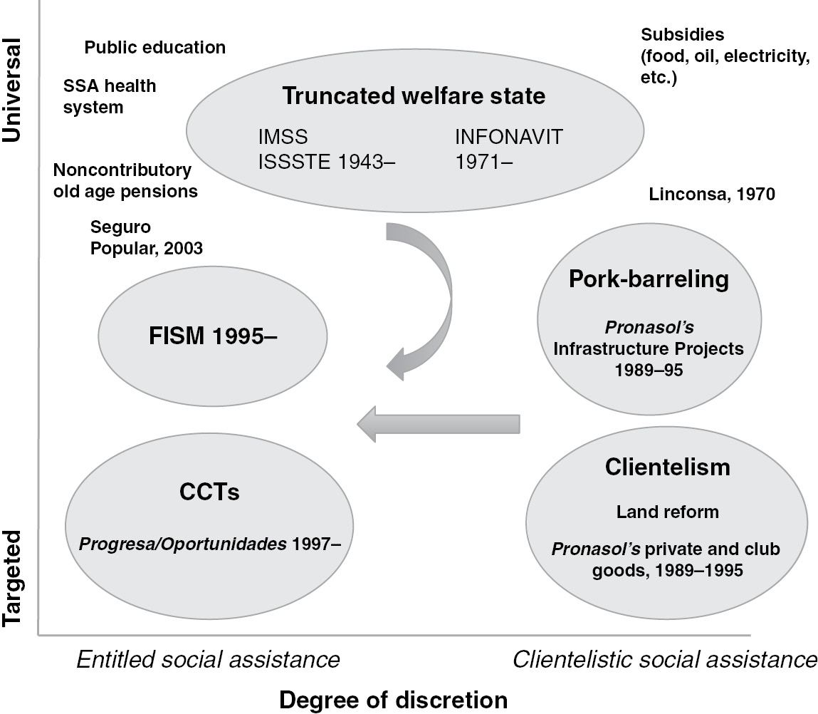
The evolution of poverty is surely related to the historical policies followed by the federal government. Figure 2.1 maps Mexico’s social policies during the twentieth century on the two dimensions of governance discussed in the previous chapter. Since the early 1940s, Mexico began to introduce social insurance schemes tied to participation in the formal labor market. Created in 1943, the Instituto Mexicano del Seguro Social (IMSS) provides insurance to nongovernment workers, including individual retirement funds, disability and life insurance, health insurance, and health services.Footnote 4 The Instituto Nacional del Fondo de Vivienda para los Trabajadores (INFONAVIT) provides subsidized housing to private sector workers. Similar benefits are provided to state employees through the Instituto de Seguridad y Seguro Social para Trabajadores del Estado (ISSSTE), which also gives financial assistance from its housing fund (FOVISSSTE).
Social protection in Mexico.

The poor remained without access to the formal social insurance system. In addition to investments in public education and health, land reform was surely the most important redistributive effort carried out by the PRI during the postrevolutionary period, up until 1991 when the era of agrarian reform was declared closed. Over the years, 60 percent of Mexico’s territory was distributed. Owing to the clientelisitc implementation of land reform, the PRI was able to amass electoral support among peasants for many decades.
In 1988 the hitherto stable hegemonic party regime experienced an electoral shock that led to a shift in social policy. The electoral shock resulted from a combination of factors. A severe economic recession – low wages, high inflation, currency instability, and underemployment in the cities – led voters to defect to the opposition. Market-oriented reforms also restricted the availability of state resources that were traditionally used to buy off party factions and electoral support. The 1988 elections made it clear that the PRI had failed to build solid clientelistic networks with the growing masses of the urban poor.
President Carlos Salinas established Pronasol with the stated intent to combat poverty.Footnote 5 Instead, as we demonstrate in this book, Pronasol was designed as an instrument for reestablishing the PRI’s electoral dominance. Pronasol sought to establish alternative party-society relationships that would go around the failing corporatist mechanisms and state bureaucracies. It soon became the cornerstone of the government’s social policy. Its resources represented, on average, 1.18 percent of GDP each year.
A large proportion of Pronasol programs involved investments in sewerage, piped water, roads, and the construction of schools and health clinics. But Pronasol also included many programs that targeted discretionary private goods to individuals or small communities – subsidized credit, scholarships, wells, livestock, construction materials, and the like. The program’s investments benefited the PRI’s core supporters and were not properly targeted to the poor.
In the 1990s, as the process of democratization unfolded, a new social assistance regime came into place. Through the randomization of the first CCT program in Mexico, Progresa‘s initial rollout from 1997 to 1999, scientific evaluations were made on the impact of the program on the welfare of the poor. The presidential administration of Vicente Fox became convinced that the program was effective; he decided to rename it and expand it into urban areas. We demonstrate in this book that beneficiaries of Progresa – and later Oportunidades – have generously rewarded incumbents at the polls.
After Vicente Fox’s victory in 2000, the program was expanded in rural areas, and extended to urban and semiurban areas using parallel criteria to select beneficiary families. For the last phase, the program was also transformed into a demand-type scheme where eligible people were no longer identified by the government, but they self-select to apply. The scope of Progresa/Oportunidades is far-reaching. At the end of 1999, Progresa covered approximately 2.6 million families, and about 40 percent of all rural families. By 2005, Oportunidades covered 5 million families, almost 70 percent rural, and the rest semiurban and urban. This meant that by the end of 2005, more than half of Mexican families in extreme poverty were receiving Oportunidades funds. The program’s budget has increased steadily since 1997, although transfers per beneficiary have decreased slightly.
Because of its progressive structure, Progresa/Oportunidades is the most propoor of all major Mexican social assistance programs. The World Bank has calculated in its public expenditure review for Mexico in 2005 that most public programs are regressive, and that public expenditure in general is slightly regressive (World Bank, 2004a). Other national programs that have been progressive are school spending (preschool, elementary and lower secondary), health clinics for the uninsured population through the ministry of health (SSA), and the Programa de Apoyos al Campo (Procampo) transfers to peasants.Footnote 6 Procampo replaced price supports for basic grains with direct cash payments. The most regressive programs have been those managed by the Public Employees Social Security Institute (ISSSTE) and support for public universities.
Despite enormous improvement in poverty alleviation under Oportunidades, the program still suffers limitations. For example, poor households are excluded from receiving transfers if there is no school or clinic in the community or within a reasonable distance, which is the case in some of Mexico’s poorest localities. Second, the continuity of the program is always at stake when there is a change in federal administration and governments are tempted to water down its targeting. Third, the transfers themselves are not generous enough to place all households in the program above the poverty line, so a substantial population remains in poverty, even after the transfer. Finally, Oportunidades is not well integrated with other social assistance programs that seek to generate better quality services and to support income-generating activities (de Janvry, Reference De Janvry2006).
Highly targeted programs may suffer important political limitations. As Pritchett (Reference Pritchett2005) explains: “If the budget for redistribution is politically determined, the impact of targeting on the poor cannot be determined by a technocratic evaluation of the hypothetical impact of a given targeting design alone; it must account for the effect of changes in the degree of targeting on the size of the budget available for redistribution. It is possible that ‘more for the poor is less for the poor’ and that the less targeted program will deliver fewer benefits for the poor” (p. 1).
CCTs can suffer underfunding. In fact, social spending is relatively low in Mexico at 9.1 percent of GDP in 2000.Footnote 7 Most of the spending goes to education and health (3.8 and 2.2 percent of GDP respectively). Social protection spending constitutes the remaining 3 percent. Around 72 percent of social protection spending is devoted to regressive programs (IMSS and ISSSTE), whereas only 27 percent (0.8 percent of GDP) goes to the better-targeted social assistance programs, including Oportunidades (Lindert and Allard, 2006).Footnote 8 Hailed as the most successful poverty alleviation program in Mexico’s history, Oportunidades made only up 0.3 percent of GDP in 2000.
2.2 The Geography of Poverty
Behind the national figures that exhibit some improvements, there are vast differences across the territorial landscape. Unpacking poverty in Mexico requires a better understanding of its relationship with geography. The central goal of our analysis is to understand the impact social programs have made on poor communities and the evolution of poverty. In the rest of this chapter, we outline the basic spatial patterns of poverty, the geography of public expenditure, and the distribution of political power across the territory.
Poverty in Mexico is highly correlated with specific topographic and climatic characteristics. A typical, extremely poor locality is generally isolated from main cities, roads, and highways. One of the most unequal countries in the world, Mexico’s social disparities are reflected in its high incidence of poverty. The poor are concentrated in rural communities. The rural poor historically have lacked basic services such as drinking water, roads, and health care, and they have suffered from hunger, malnutrition, and preventable disease.
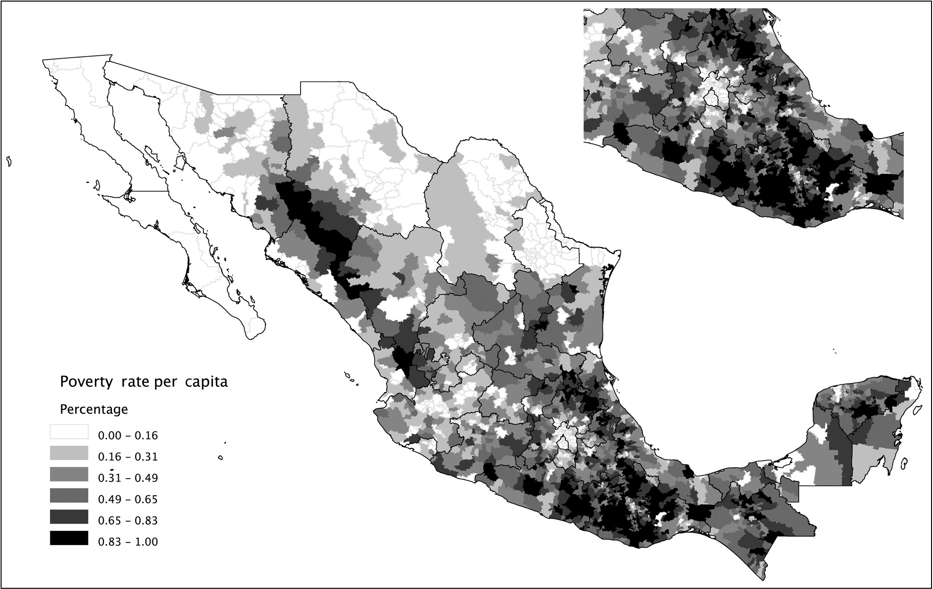
Figure 2.2 maps poverty across Mexico. The map uses the CONEVAL computation of nutritional poverty (i.e., a poverty line drawn at the minimum caloric intake necessary for survival) at the municipal level in 2000. It highlights the prevalence of extremely poor households across Mexico, with a spatial distribution showing that poverty is most concentrated in rural areas.
Share of population living under nutritional poverty line (CONEVAL), 2002.
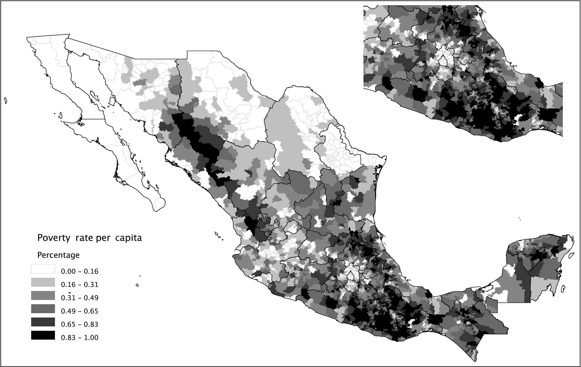
There is an undeniable statistical correlation between the patterns of poverty and destitution displayed by the map in Figure 2.1 and a set of geographic variables. The rural poor in Mexico tend to live in less accessible and hospitable places. Their settlement patterns usually reflect inherited and long-standing historical processes that have also generated the borders separating jurisdictions. The South is poorer than the North, and it also has the highest concentration of indigenous peoples. Southern states such as Chiapas, Yucantán, Oaxaca, Guerrero are among the poorest. Puebla, Michoacán, and areas of Veracruz also exhibit high incidence of poverty. In the North poverty is concentrated la Sierra Tarahumara, an area of the Sierra Madre Occidental inhabited by the Tarahumaras. Rural Western Central Mexico in Nayarit, Durango, Jalisco, and Zacatecas is also impoverished.
Gallup et al. (Reference Gallup, Sachs and Mellinger2001, Reference Gallup, Gaviria and Lora2003) and Sachs (Reference Sachs2005) have argued that geography plays a key role in development. For example, landlocked countries tend to grow at a slower rate than those with coastal access and navigable rivers. Across the world, it is well known that latitude is correlated with per capita GDP levels (Sachs, Reference Sachs2005). We know that institutional and historical processes also shape the evolution of well-being (Acemoglu and Robinson, Reference Acemoglu and Robinson2006); and that geography is not destiny (Gallup et al., Reference Gallup, Gaviria and Lora2003). Yet poverty profiles are inevitably linked to the geographical characteristics of the territories where poor people live. This geographic relationship presents a methodological opportunity. Since human agency can only change geographic attributes at the margin (roads, bridges and tunnels can be built, swamps can be drained and rivers dammed, but mountains cannot be moved), geographic attributes are extremely good predictors of the spatial distribution of poverty.
The most striking aspect of Mexico’s natural geography is its extreme variation. And those variations are highly correlated with poverty. Mexico provides a contrast to the findings by Gallup et al. (Reference Gallup, Sachs and Mellinger2001) that population and economic activity tend to concentrate on coasts and major waterways. The overwhelming majority of Mexican municipalities are landlocked and the population is not concentrated in coastal areas. The development of Mexico’s transportation infrastructure since the nineteenth century has provided most municipalities with access to both railroads and major roads (within an average of twenty-three kilometers and five kilometers, respectively).
Table 2.2 presents an ordinary least squares (OLS) regression of several indicators of poverty and development on a selection of geographic variables.Footnote 9 The dependent variables are all normalized into z scores with a mean of 0 and a standard deviation of 1 to make it possible to compare the impact of various geographic features across regressions (although each of the indicators is constructed with different underlying data). To measure poverty, we employ three alternative indicators. The first indicator we use is the nutritional poverty headcount index presented in Figure 2.2. A second indicator measures the relative deprivation of municipalities in 1990. The index combines characteristics of households, including access to public services such as sewage systems, drinking water and electricity, access to housing construction materials, and individual traits such as literacy and earnings according to the 1990 census. The final dependent variable is the Human Development Index (HDI) calculated by UNDP on the basis of 2000 census data.Footnote 10
| 1 | 2 | 3 | 4 | 5 | 6 | |
|---|---|---|---|---|---|---|
| Poverty headcount w/ Natural Geography | Poverty headcount w/ Natural Geography | Marginality index w/ Natural Geography | Marginality index w/ Human Geography | HDIw/ Natural Geography w/ Natural Geography | HDIw/ Human Geography w/ Human Geography | |
| Spatial lag | 0.265 | 0.169 | 0.174 | 0.117 | 0.123 | 0.06 |
| (0.054)** | (0.043)** | (0.057)** | (0.048)* | (0.062)* | (0.054) | |
| North | –0.963 | –0.706 | –0.97 | –0.755 | 1.001 | 0.74 |
| (Km/1000) | (0.069)** | (0.070)** | (0.069)** | (0.071)** | (0.071)** | (0.072)** |
| East | 0.509 | 0.568 | 0.356 | 0.444 | –0.275 | –0.398 |
| (Km/1000) | (0.054)** | (0.051)** | (0.055)** | (0.053)** | (0.054)** | (0.054)** |
| Temperature | –0.014 | –0.004 | –0.015 | –0.006 | 0.012 | 0.005 |
| (°C) | (0.003)** | (0.002) | (0.003)** | (0.003)* | (0.003)** | (0.003) |
| Rainfall | 0.762 | 0.905 | 0.963 | 0.997 | –0.813 | –0.851 |
| (Meters) | (0.100)** | (0.081)** | (0.099)** | (0.085)** | (0.099)** | (0.084)** |
| Coastline | –0.697 | –0.504 | –0.772 | –0.643 | 0.84 | 0.678 |
| (1= coast/border) | (0.073)** | (0.070)** | (0.074)** | (0.071)** | (0.070)** | (0.070)** |
| Rugged Terrain | 0.95 | 0.599 | 0.998 | 0.642 | –0.814 | –0.484 |
| (st. dev. Km) | (0.377)* | (0.292)* | (0.390)* | (0.291)* | (0.323)* | (0.249) |
| Altitude | –0.893 | –0.482 | –1.067 | –0.657 | 0.791 | 0.396 |
| (km) | (0.375)* | (0.291) | (0.388)** | (0.291)* | (0.322)* | (0.249) |
| Distance City | 0.002 | 0.002 | –0.003 | |||
| (Km) | (0.000)** | (0.001)** | (0.000)** | |||
| Distance Rail | 0.004 | 0.004 | –0.005 | |||
| (km) | (0.001)** | (0.001)** | (0.001)** | |||
| Distance Road | 0.018 | 0.019 | ||||
| (km) | (0.001)** | (0.002)** | (0.002)** | |||
| Population | –0.222 | –0.14 | 0.159 | |||
| (Log) | (0.012)** | (0.014)** | (0.014)** | |||
| Area | 0.044 | 0.038 | ||||
| (Km2/1000) | (0.010)** | (0.011)** | (0.009)** | |||
| Constant | –0.432 | 0.736 | –0.041 | 0.405 | –0.003 | –0.504 |
| (0.160)** | (0.192)** | (0.163) | (0.215) | (0.163) | (0.221)* | |
| Observations | 2425 | 2375 | 2425 | 2375 | 2425 | 2375 |
| R-squared | 0.33 | 0.57 | 0.3 | 0.48 | 0.27 | 0.48 |
Note: Robust standard errors in parenthesis.
* Significant at the 5% level; ** significant at the 1% level.
The independent variables include a correction for spatial autocorrelation (poverty in neighboring municipalities) latitude, longitude, altitude, rainfall, and temperature. Mexico is a particularly mountainous country, so we calculated from the data on altitude the ruggedness of each municipality’s terrain (measured as the standard deviation of altitude). This measure indicates how physically inaccessible a place is. We calculated the number of major rivers crossing a municipality and whether there was a major lake. The coastline variable detects access to the sea. Given the peculiarities of Mexico’s highly permeable border with the United States, we coded municipalities on the northern border also as coastline.
The land area of the municipality reflects a measure of size, while population indicates the relative importance of municipalities. Population density combines both of these indicators, reflecting to a large extent the degree of urbanization. Finally we calculated four indicators reflecting accessibility to markets: distance to major highways, railroad tracks, cities of more than 100,000 inhabitants and Mexico City. All the distance variables were calculated, using a Euclidean metric, to the closest point on the border of the jurisdiction.
The table explicitly states in its headings that the coefficients should be read as suggestive of correlations to poverty, not of a causal relationship in which the geographic variables “explain” or produce specific outcomes of poverty and development.Footnote 11 Two estimations are reported for each index, one that includes only variables of natural or physical geography (latitude, longitude, temperature, rainfall, coastline, altitude and terrain ruggedness), and the other that includes what we call “human geography,” indicating that the variables of distance, population and even land area are the product of demographic, socioeconomic, and political choices, accumulated over several decades and even centuries.
These results allow us to identify a distinctive geographic profile of poverty in Mexico. Estimations 1, 3, and 4 show that a third of the variance, as reflected by the R2 statistic, is accounted for by natural geography variables alone. There is a powerful North-South divide that is evident in the latitude variable. The size of the effect is substantial. Using the coefficients from estimation 5, if we take municipalities with identical characteristics, except that one is located a thousand kilometers farther to the north, that sole difference would yield a change of one standard deviation in the HDI z score. The estimation also reveals an east-west cleavage. One thousand kilometers more to the east yields a poverty headcount index one-half a standard deviation larger.
Rainfall is statistically significant through all the estimations, including those with human geography variables, suggesting that places with more rainfall tend to be characterized by greater deprivation. Rugged terrain is significant at the 95 percent level, implying the presence of geographic poverty traps in areas made remote and difficult to access due to topography (Jalan and Ravaillon, Reference Jalan and Ravallion2002; Bloom et al., Reference Bloom, Canning and Sevilla2003). The poor in Mexican municipalities with inaccessible terrain have a hard time migrating out of those places or readily move their accumulated human capital or assets beyond a threshold that allows them to increase their productivity.Footnote 12
Temperature and altitude are statistically significant only when variables linked to human geography are not included in the estimation, which suggests that the correlation of these environmental conditions with poverty is less pronounced in the presence of human activities that facilitate the movement of goods and people across a territory.
The inclusion of the human geography variables increases the power of the regressions significantly. More than half of the variance in the distribution of poverty is accounted for when human geography is taken into account, as indicated by the R2 statistic. The equivalent statistics for the marginality index and the HDI are similar. The human geography variables are all significant in the expected direction. When a municipality is far from a large city, has no nearby railroad line and is not linked to the rest of the country through the highway network, its population is significantly poorer. Larger municipalities in terms of land area tend to be poorer, but more population is associated with less poverty, which in the end means that places with greater population density (i.e., more urban concentrations) exhibit less poverty.
When controlling for human geography, the variables related to the topography of the territory either cease to be statistically significant or reduce their association with poverty, which is consistent with the view that infrastructure and urbanization allow people to overcome poverty. Government action or inaction can hence have a large impact on poverty alleviation.
Among the human geography variables, the distance to railroads and the land size of municipalities have been virtually fixed over the past century. Most railroads were built in the nineteenth century (Coatsworth, Reference Coatsworth1976), and the municipal subdivision has only changed marginally since 1917 (Blum and Diaz-Cayeros, Reference Blum and Diaz-Cayeros2002). Most cities with more than 100,000 inhabitants were established as large urban concentrations in colonial times. According to Tanck de Estrada (Reference Tanck de Estrada2005) there were around twenty Spanish cities and “villas” in 1800, as distinct from the so-called Indian pueblos. Spanish cities were the centers of power and wealth in the colonial period. Although much has changed since then, today’s large cities were established in the late colonial period, with the exception of cities on the northern border and some coastal ports that have blossomed as tourist centers in the past few decades.
On the contrary, other human geography variables have been changing rapidly during the past decades. Demographic patterns are not exogenous to the social, economic, or political processes of both the recent and the distant past. These sociopolitical processes include dislocations produced by social upheaval at the beginning of the twentieth century, massive urban migration since the 1960s, and the large-scale emigration to the United States since the 1980s.
National highway construction in Mexico began in the 1920s, and the new construction often followed old colonial routes (Ortiz Hernán, Reference Ortiz Hernán1994). But there has been a steady expansion of road networks since the 1960s, with a recent boom in highway construction in the 1990s funded by joint private-public ventures. Among the geographical variables included in our estimations, highways are arguably the most reflective of recent government activity.
The location, climate, and terrain of a municipality are important predictors of poverty levels. Our results suggest that poverty is determined by a combination of human agency and geographic conditions, but is driven more by the latter. Again, the associations shown in these estimations are not necessarily causal. In fact, the social, economic, and political processes captured by the geographic variables, particularly the ones shaped by human agency, are very likely the consequence of poverty as much as the cause. Teasing out the links of causality goes beyond the scope of this chapter.
2.3 Strategies for Public Goods Provision and Poverty Alleviation
The accumulated experience of two decades of poverty relief spending in Mexico affords a unique opportunity to compare and contrast poverty- alleviation efforts, particularly with regard to differences between discretionary and formula-based programs, targeted and universal approaches, and centralized and decentralized decision making. It also provides insights into the ways in which local politics influences the implementation and allocation of funds across households and political jurisdictions. This book compares social spending strategies in all of Mexico’s municipalities that span three presidential terms.
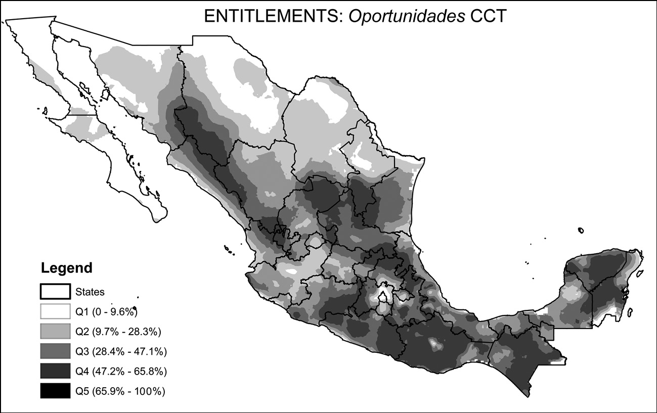
Figure 2.3 shows the geographic distribution of the funds for Pronasol, FISM and Progresa/Oportunidades at the municipal level. The maps are organized into rows and columns corresponding to Figure I.1. The first two maps show nondiscretional or formula-based antipoverty funds distributed to municipalities while the maps in the next page discretional programs. The top map shows funds for localities (earmarked and block grants in the case of FISM and public goods constituting pork-barrel appropriations for Pronasol); while the bottom map depicts programs targeted to individuals (through entitlement-based transfers in the case of Oportunidades and in a clientelistic manner in the case of Pronasol).
The geography of poverty relief transfers in Mexico, 1989–2005.
Note: Pronasol average data for 1989–1994; FISM data for 2000; Oportunidades coverage for 2005. All figures are per capita in real pesos of 1994 or share of population for Oportunidades (1 USD = 3.3 MXP).
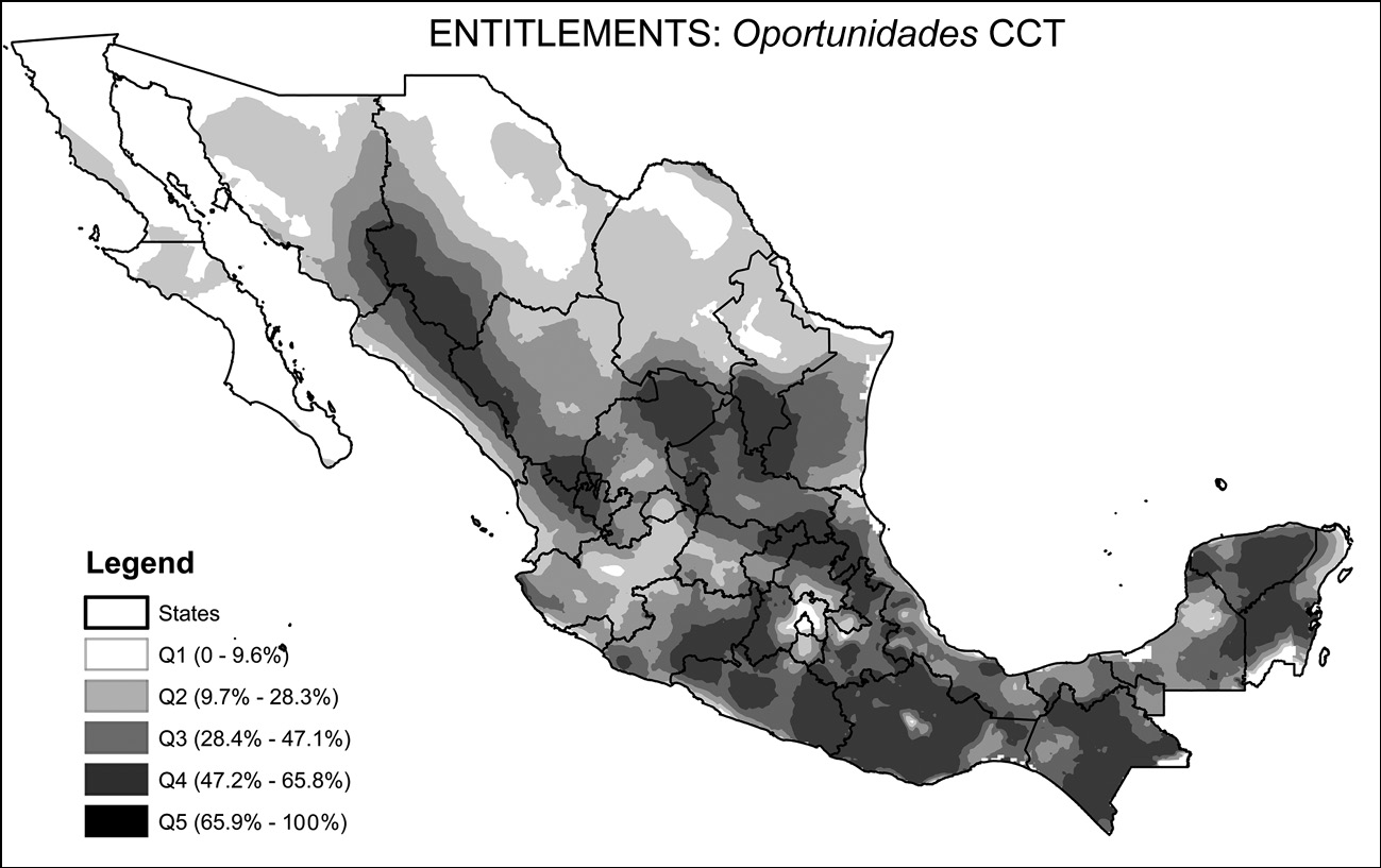
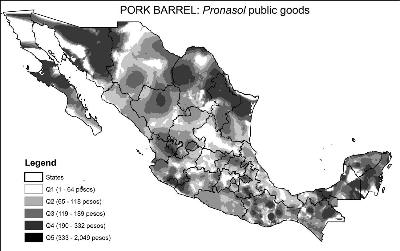
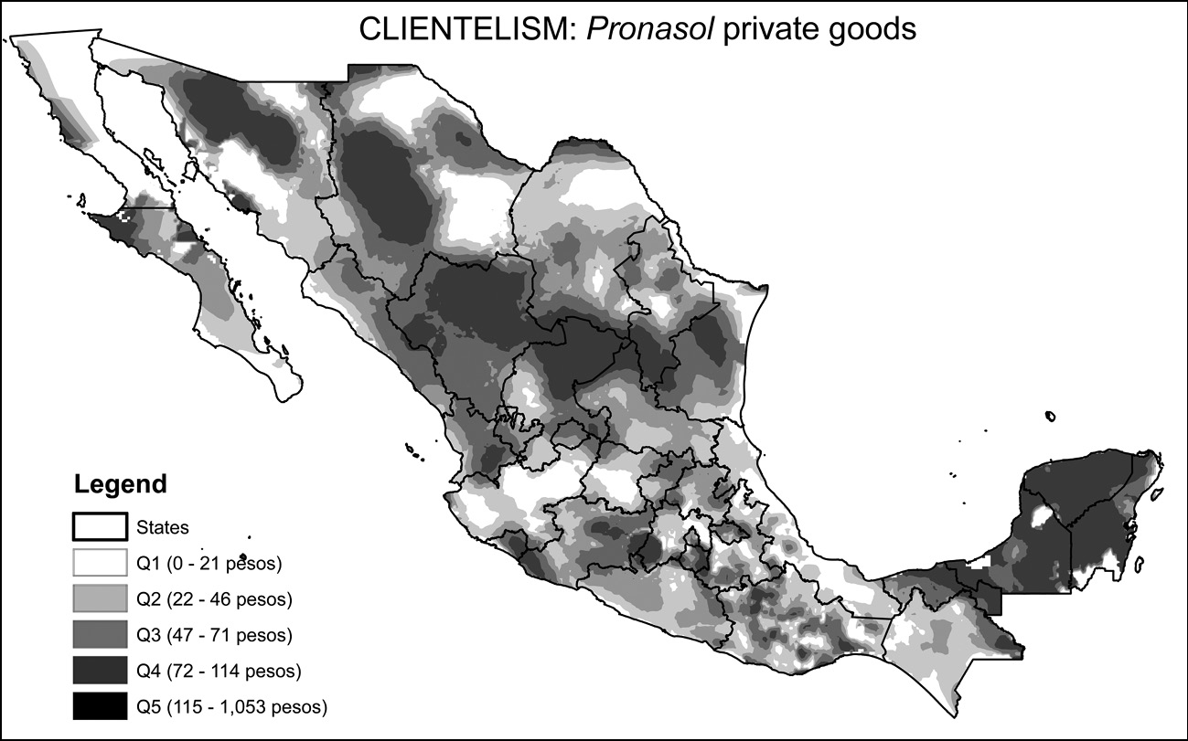
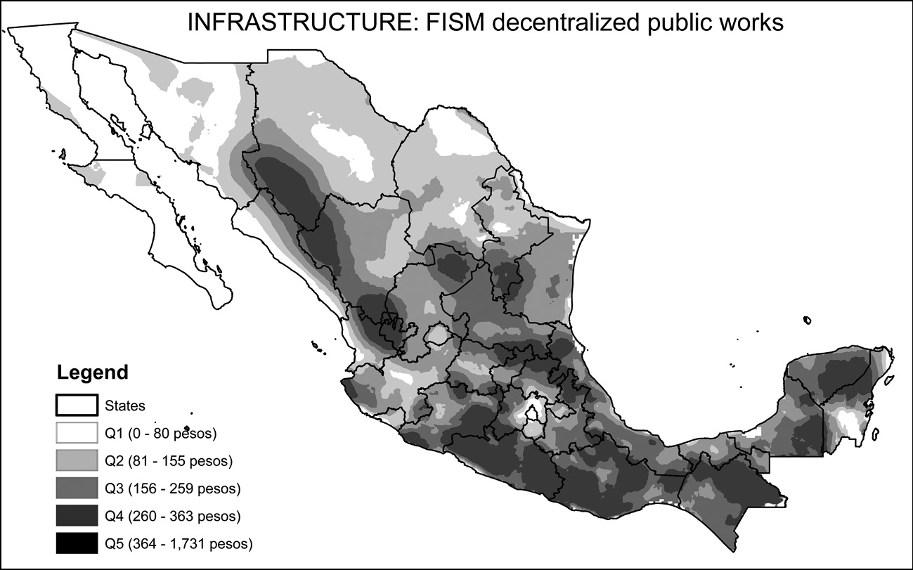
The map in the bottom of the second page shows the mean per capita allocation of Pronasol funds for private goods, measured in 1994 pesos, for the 2,417 municipalities in Mexico at the time, during the six years of the program (1989–1994).Footnote 13 Pronasol was made up of more than twenty programs, which we reclassified into projects providing private goods and projects providing public goods.Footnote 14 The map in the top row of that discretional column shows the public goods allocations of Pronasol for the same time period. The map in the top left cell shows the mean allocation of municipal social infrastructure funds (FDSM/FISM) from 1996 to 2000, also in real per capita terms.Footnote 15 The final map in the figure in the bottom left cell shows the mean per capita allocation of Oportunidades funds from 2001 to 2005.Footnote 16
In order to render the visualization of highly disaggregated data more effective, the maps show smoothed surfaces of spending estimated in similar fashion to temperature or rainfall maps. This is created through a third degree spatial polynomial of spending over 30 neighboring municipalities in the territory (in the rainfall analogy, this is similar to having 2,430 weather stations, and the surface is generated by something similar to an average of their readings over the territory). The isolines shading the maps establish contours of territory with similar levels of funding, just like in a typical topographic map.
Despite their widely different levels of development, all municipalities in Mexico received at least some funds from each program. The different criteria for selecting beneficiaries are reflected in the geographic patterns observed in the figure. The magnitude of the funds involved in each program varies widely. Pronasol public goods comprised the largest appropriations, followed by FISM. Oportunidades funding is substantially smaller than the private goods component of Pronasol, which was less than half of the public goods allocation. The programs were different from one another in several respects: Pronasol included funding geared towards large infrastructure investment in highways, sizeable transfers devoted to financing local public goods and transfers to individuals and organized groups. FISM has a narrower scope, providing direct municipal financing for local public goods selected and administered by local governments. Progresa provided CCTs to individual households in rural areas only, while Oportunidades expanded the rural coverage of Progresa to urban beneficiaries using the same basic design of the CCT program.
The most notable feature to emerge from a visual comparison of the maps is the marked difference in the geographical distribution of funds. An even shading of any map would mean that funds were distributed in an equal per capita amount across municipalities, rather than targeted to poorest localities. Maps with contrasting dark and light shades indicate more unequal allocations or, in this context, better targeted allocations. Areas of the country with greater concentrations of poor households should deservedly have more funds allocated to them than richer regions.
A comparison of the mapping of poverty and the distribution of social program outlays (Figures 2.2 and 2.3) suggests that the program that most closely matched poverty profiles across space is Oportunidades. FISM funds also show a remarkably similar distribution to the one found in a poverty headcount ratio. In contrast, private goods provision in the Pronasol program was concentrated in Northern Mexico and the Yucatán peninsula, not necessarily the poorest areas of the country. Very low allocations of those funds were observed in the state of Veracruz on the Gulf coast, and in the western highlands, particularly in the state of Jalisco. The distribution of Pronasol public goods is somewhat distinct: large amounts of funds were allocated in some Northern states, while smaller ones went to central areas, particularly the region North of Mexico City. An assessment of whether there is enough of a match between the territorial distribution of public funds and the mapping of poverty is developed in future chapters.
2.4 The Political Landscape
Our focus in this book is on how social programs are shaped by political and electoral considerations, and how these programs impact welfare and voting decisions. In much of the analysis of the book we take into account the partisan identity of incumbents at the municipal level and the degree of competition they face. The complexity of capturing the political landscape of a country is reduced, to some extent, by the existence of relatively nationalized political parties. Through patterns of observed electoral support we are able to know something about the configuration of political preferences across the territory, which can be used as convenient shorthand for more complicated interactions between individual politicians, communities, and voters.
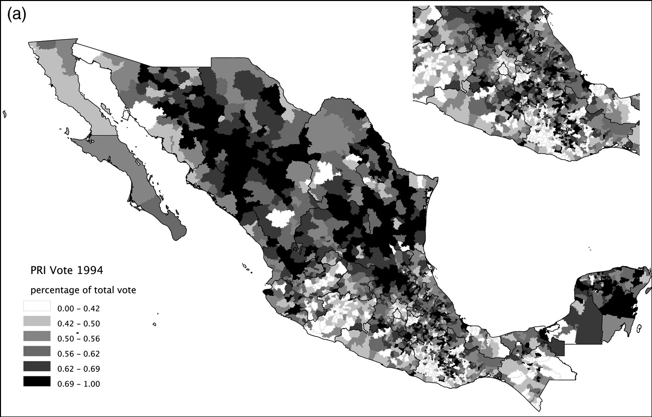
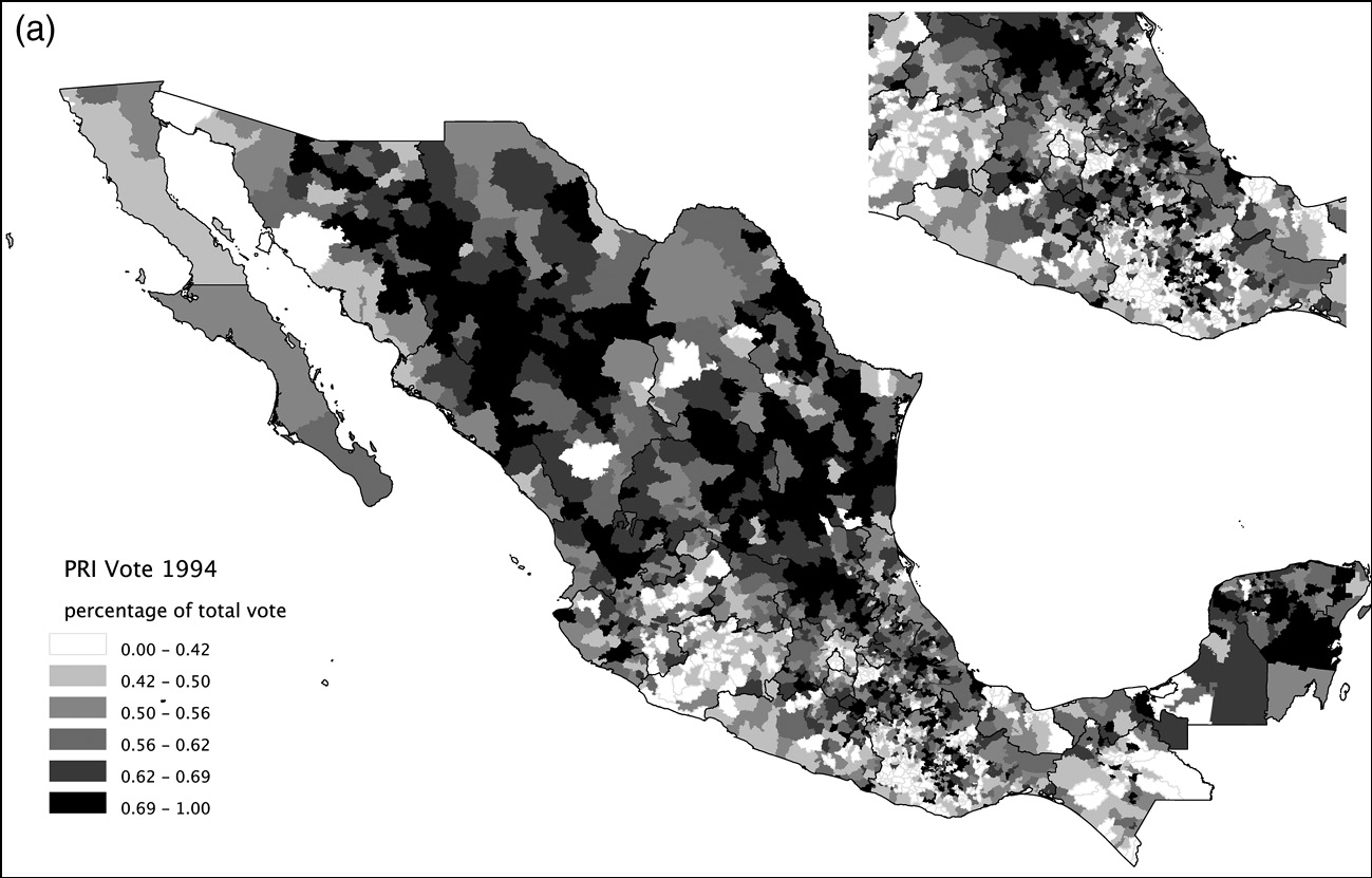
The first map shown in Figure 2.4 displays the support for the PRI in the 1994 federal elections, which yielded a PRI victory despite strong challenges from both the PAN and the PRD. The first thing to note is that, although the party no longer enjoyed the levels of electoral support it had grown accustomed to in the hegemonic era, it still commanded very large majorities in most municipalities in the country. Shaded in white are places where the PRI candidate Ernesto Zedillo received less than 42 percent of the vote; and in dark grey the municipalities where he got more than 50 percent of the vote. The municipal map visually exaggerates the importance of northern support due to the larger territorial size of municipalities in that region, but nevertheless it attests to widespread support for the PRI throughout the country, with the exception of greater Mexico City, the western highlands and parts of the south. A striking correlation is apparent between the geography of Pronasol expenditures displayed in Figure 2.3 and the geography of PRI support. This correlation will be systematically explored in subsequent chapters where we will develop a measure of PRI core support using long-term electoral returns from 1970 until 1988 that are exogenous to later expenditures. The positive correlation between this measure of PRI core support and expenditures will be the subject of our statistical models in Chapter 4.
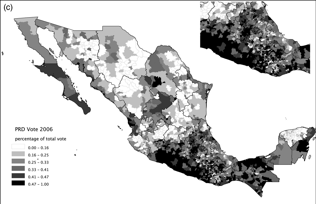
Electoral geography.
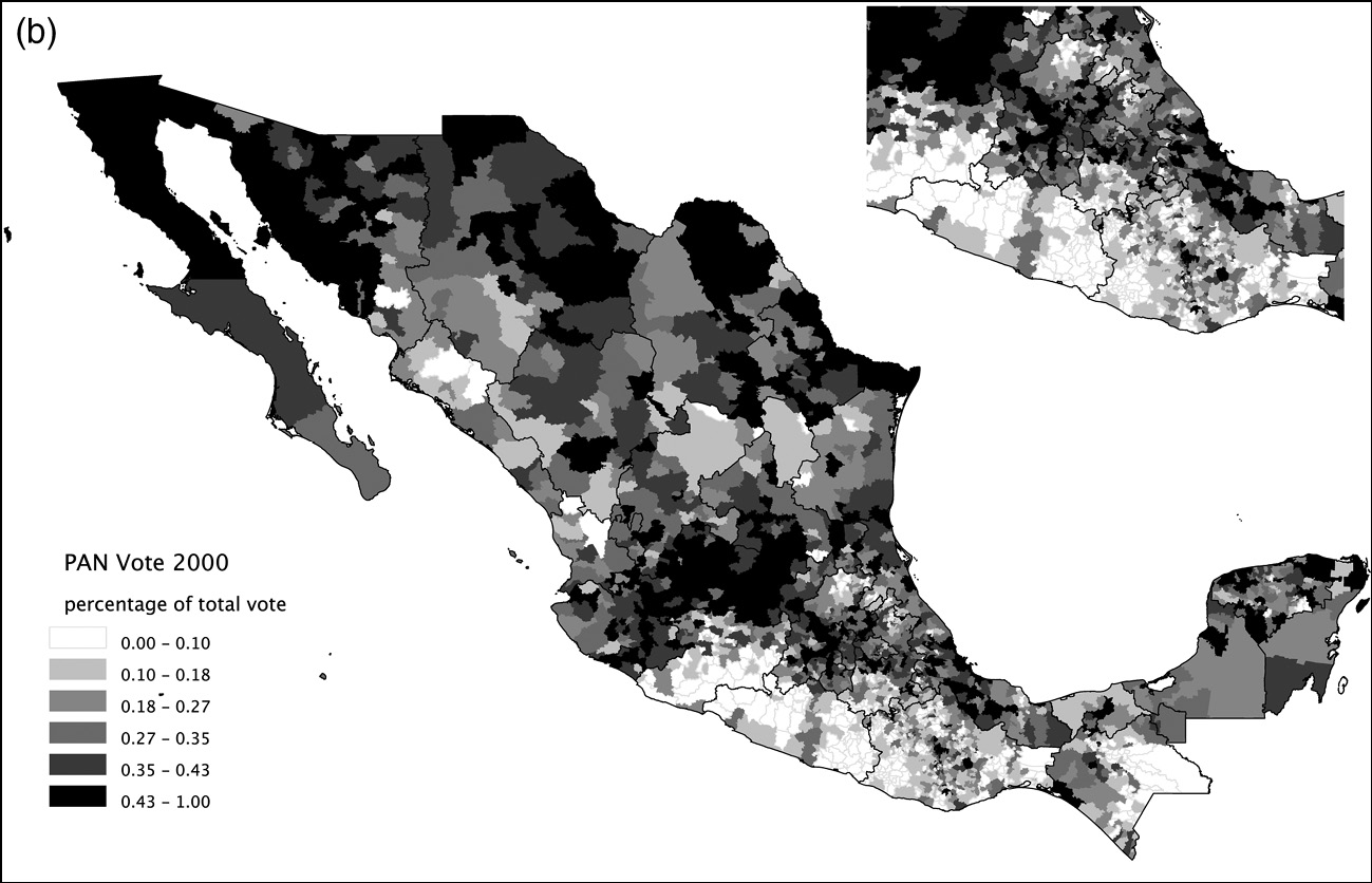
The second map shows the distribution of vote shares for the PAN in the 2000 elections, with the general shading indicating some regional contrasts in support. The highest vote shares for the PAN appear in the western highlands, the northern border and scattered municipalities in central Mexico. The party appears extremely weak, with vote shares below10 percent, in the south, where most of the poor concentrate. In contrast to the PRI map above it, the levels of support for the PAN across municipalities were much lower than those enjoyed by the PRI, even in elections that the ruling party lost. A simple visual comparison between the poverty map in Figure 2.2 and the PAN’s electoral returns in 2000 displayed in Figure 2.4 highlights its scant support among the rural poor when it won the presidency in 2000. In Chapter 8 it will become apparent how the PAN was able to increase its electoral base among the poor in the 2006 presidential elections, expanding Oportunidades during Vicente Fox’s presidential term.
The third map shows levels of electoral support of the PRD in the 2006 elections, which candidate Andrés Manuel López Obrador lost by a small margin based on officially sanctioned results. We use 2006 to map the PRD’s vote because that is the year of the left’s strongest performance in national elections. In the Southern half of the country, PRD strength appears to be highly correlated with the distribution of poverty in Figure 2.3. In the Western highlands and the North, that is not the case.
Although the three maps reflect different presidential elections spanning twelve years, taken together the maps tell an important story about the character of electoral competition in Mexico. From the mid-1990s onward, partisan competition in federal elections has strengthened, but in clearly defined territorial patterns. The PRI is electorally competitive throughout the country, generally facing challenges from the PAN in the North and West and from the PRD in the South. The PAN and the PRD, however, rarely compete against each other in any particular municipality, state, or region. Truly three-party elections are mostly observed in the central region of the country, especially in greater Mexico City, and in some urban districts in the rest of the country.
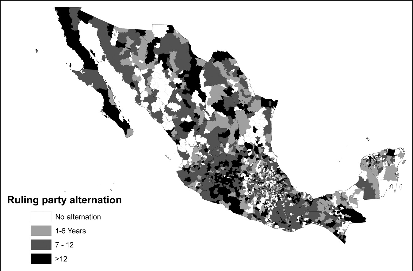
While the federal electoral results provide a good overview of the conditions that make Mexican electoral politics so vibrant and competitive, it is important to note that democratization did not just come about as a national process. Local processes of alternation in political power, where the PRI had no other choice but to recognize its defeats in municipal and eventually state-level electoral contests preceded the transition to democracy. Figure 2.5 provides an indicator of the process of democratization from a local perspective, by showing the years since an alternation in mayoral races taking place in each of the municipalities.
Municipal democracy: years since party alternation.

Alternation at the local level provides an unambiguous indicator that the PRI no longer held a monopoly of representation, even if voters may have decided to allow that party to return to political office in subsequent elections after its defeat. The general pattern displayed in the map shows, first, that virtually all municipalities have had some alternation by 2006. In this sense,despite the deep entrenchment of party bosses and machines in various regions, democratization from below is undeniable.
Second, democratization from below does not seem to obey a particular territorial logic or be simply driven by modernization processes. While in the early 1990s capital cities in the states and relatively rich municipalities were more likely to vote against the PRI, as democratization advanced electoral victories of the opposition were observed throughout the country.
It is perhaps not so surprising, in the context of these electoral challenges, that PRI governments strategically used the distribution of poverty relief resources. The political imperative of the party was to remain in office, and prevent further erosion, in the face of vigorous competition by parties. The next chapter moves to the task of providing a theory of how politicians address electoral threats using the distribution of transfers to voters as a way to buy off political support; the chapter after that assesses the success of that strategy for the case of Pronasol during the Salinas years.