3.1 Leading-order boundary-layer solution

In order to satisfy the stress-free conditions (2.6a,b ), there must be a boundary layer close to the free surface where viscous effects are non-negligible. Asymptotic expansions introduced in Moore et al. (Reference Moore, Ockendon, Ockendon and Oliver2014) show that the relevant scalings are

(3.3) $$\begin{eqnarray}\left.\begin{array}{@{}c@{}}n=\unicode[STIX]{x1D700}{\tilde{n}},\quad u=1+\unicode[STIX]{x1D700}\tilde{u} ,\quad v=\unicode[STIX]{x1D700}^{2}\tilde{v},\quad p=\unicode[STIX]{x1D700}\tilde{p},\quad h=\unicode[STIX]{x1D700}^{2}\tilde{h},\quad \unicode[STIX]{x1D70F}_{ss}=\unicode[STIX]{x1D700}\tilde{\unicode[STIX]{x1D70F}}_{ss},\\ \unicode[STIX]{x1D70F}_{sn}=\tilde{\unicode[STIX]{x1D70F}}_{sn},\quad \unicode[STIX]{x1D70F}_{nn}=\unicode[STIX]{x1D700}\tilde{\unicode[STIX]{x1D70F}}_{nn}.\end{array}\right\}\end{eqnarray}$$

We substitute these into (2.1)–(2.6) and expand as asymptotic series in powers of $\unicode[STIX]{x1D700}$ . To leading order in the boundary layer, we see that

(3.4a-c ) $$\begin{eqnarray}\displaystyle & \displaystyle \frac{\unicode[STIX]{x2202}\tilde{p}_{0}}{\unicode[STIX]{x2202}{\tilde{n}}}=\unicode[STIX]{x1D705},\quad \frac{\unicode[STIX]{x2202}\tilde{u} _{0}}{\unicode[STIX]{x2202}s}=-\frac{\unicode[STIX]{x2202}\tilde{p}_{0}}{\unicode[STIX]{x2202}s}+\frac{\unicode[STIX]{x2202}^{2}\tilde{u} _{0}}{\unicode[STIX]{x2202}{\tilde{n}}^{2}},\quad \frac{\unicode[STIX]{x2202}\tilde{u} _{0}}{\unicode[STIX]{x2202}s}+\frac{\unicode[STIX]{x2202}\tilde{v}_{0}}{\unicode[STIX]{x2202}{\tilde{n}}}=0, & \displaystyle\end{eqnarray}$$

subject to

(3.5a-c ) $$\begin{eqnarray}\displaystyle & \displaystyle \tilde{p}_{0}(s,0)=0,\quad \frac{\unicode[STIX]{x2202}\tilde{u} _{0}}{\unicode[STIX]{x2202}{\tilde{n}}}(s,0)=\unicode[STIX]{x1D705},\quad \tilde{v}_{0}(s,0)=\frac{\text{d}\tilde{h}_{0}}{\text{d}s}, & \displaystyle\end{eqnarray}$$

on the free surface, and

(3.6a,b ) $$\begin{eqnarray}\displaystyle \tilde{u} _{0}\rightarrow 0\quad \text{as }s\rightarrow -\infty ,\quad \tilde{u} _{0}\sim -\unicode[STIX]{x1D705}{\tilde{n}}\quad \text{as }{\tilde{n}}\rightarrow \infty . & & \displaystyle\end{eqnarray}$$

Clearly, from (3.4a ), (3.5a ),

(3.7) $$\begin{eqnarray}\displaystyle \tilde{p}_{0}=\unicode[STIX]{x1D705}{\tilde{n}}. & & \displaystyle\end{eqnarray}$$

Upon writing $\tilde{u} _{0}=-\unicode[STIX]{x1D705}{\tilde{n}}+\tilde{w}$ to reduce (3.4b ) to the heat equation, we employ a Fourier transform in $s$ to deduce that

(3.8) $$\begin{eqnarray}\displaystyle & \displaystyle \tilde{w}=-\frac{2}{\sqrt{\unicode[STIX]{x03C0}}}\int _{-\infty }^{s}\frac{\unicode[STIX]{x1D705}(\unicode[STIX]{x1D709})}{\sqrt{s-\unicode[STIX]{x1D709}}}\exp \left(\frac{-{\tilde{n}}^{2}}{4(s-\unicode[STIX]{x1D709})}\right)\,\text{d}\unicode[STIX]{x1D709}. & \displaystyle\end{eqnarray}$$

It is straightforward to show that, provided the curvature decays upstream, $\tilde{w}$ is exponentially small as ${\tilde{n}}\rightarrow \infty$ .

Finally, we can find the transverse velocity, $\tilde{v}_{0}$ , by integrating the continuity equation, (3.4c ), and applying the linearised kinematic boundary condition, (3.5c ), on the free surface. However, the pertinent information, as previously deduced in Moore et al. (Reference Moore, Ockendon, Ockendon and Oliver2014), is that, in the far field, we have

(3.9) $$\begin{eqnarray}\displaystyle & \displaystyle \tilde{v}_{0}=\frac{\text{d}\unicode[STIX]{x1D705}}{\text{d}s}\frac{{\tilde{n}}^{2}}{2}+\frac{\text{d}\tilde{h}_{0}}{\text{d}s}+2\unicode[STIX]{x1D705}+\text{exp. small terms} & \displaystyle\end{eqnarray}$$

as ${\tilde{n}}\rightarrow \infty$ . This gives us a matching condition for the transverse velocity in the $O(\unicode[STIX]{x1D700}^{2})$ -problem in the outer region.

3.2 Second-order boundary-layer solution

In order to close the problem and find an equation for the correction to the free-surface location, $\tilde{h}_{0}$ , we also need a matching condition for the pressure, which means we must proceed to the next order in our boundary-layer analysis.

At $O(\unicode[STIX]{x1D700})$ in (2.2), we have

(3.10) $$\begin{eqnarray}\displaystyle & \displaystyle -2\unicode[STIX]{x1D705}\tilde{u} _{0}+\unicode[STIX]{x1D705}^{2}{\tilde{n}}=-\frac{\unicode[STIX]{x2202}\tilde{p}_{1}}{\unicode[STIX]{x2202}{\tilde{n}}}, & \displaystyle\end{eqnarray}$$

subject to the $O(\unicode[STIX]{x1D700})$ -form of the normal stress boundary condition, (2.6b ),

(3.11) $$\begin{eqnarray}\displaystyle & \displaystyle \tilde{p}_{1}+\tilde{h}_{0}\frac{\unicode[STIX]{x2202}\tilde{p}_{0}}{\unicode[STIX]{x2202}{\tilde{n}}}=0\quad \text{on }{\tilde{n}}=0. & \displaystyle\end{eqnarray}$$

Recalling that $\unicode[STIX]{x2202}\tilde{p}_{0}/\unicode[STIX]{x2202}{\tilde{n}}=\unicode[STIX]{x1D705}$ , we find that the second-order boundary-layer pressure is

(3.12) $$\begin{eqnarray}\displaystyle & \displaystyle \tilde{p}_{1}=-\frac{3\unicode[STIX]{x1D705}^{2}{\tilde{n}}^{2}}{2}-\unicode[STIX]{x1D705}\tilde{h}_{0}+2\unicode[STIX]{x1D705}\left[\tilde{w}^{\ast }-\int _{{\tilde{n}}}^{\infty }\tilde{w}(s,\unicode[STIX]{x1D708})\,\text{d}\unicode[STIX]{x1D708}\right], & \displaystyle\end{eqnarray}$$

where, from (3.8),

(3.13) $$\begin{eqnarray}\displaystyle & \displaystyle \tilde{w}^{\ast }=\int _{0}^{\infty }\tilde{w}(s,\unicode[STIX]{x1D708})\,\text{d}\unicode[STIX]{x1D708}=-2\int _{-\infty }^{s}\unicode[STIX]{x1D705}(\unicode[STIX]{x1D709})\,\text{d}\unicode[STIX]{x1D709}. & \displaystyle\end{eqnarray}$$

In particular, the far-field expansion of the $O(\unicode[STIX]{x1D700})$ -pressure is given by

(3.14) $$\begin{eqnarray}\displaystyle & \displaystyle \tilde{p}_{1}=-\frac{3\unicode[STIX]{x1D705}^{2}{\tilde{n}}^{2}}{2}+\unicode[STIX]{x1D705}(2\tilde{w}^{\ast }-\tilde{h}_{0})+\text{exp. small terms} & \displaystyle\end{eqnarray}$$

as ${\tilde{n}}\rightarrow \infty$ .

3.3 Second-order inviscid problem

We now have enough information to solve for both $\unicode[STIX]{x1D719}_{1}$ and $\tilde{h}_{0}$ . Following Moore et al. (Reference Moore, Ockendon, Ockendon and Oliver2014), the second-order velocity potential and pressure in the inviscid region satisfy the Laplace and Bernoulli equations

(3.15a,b ) $$\begin{eqnarray}\displaystyle & \displaystyle \unicode[STIX]{x1D6FB}^{2}\unicode[STIX]{x1D719}_{1}=0,\quad p_{1}+\left[\left(\frac{1}{1+\unicode[STIX]{x1D705}{\tilde{n}}}\right)^{2}\frac{\unicode[STIX]{x2202}\unicode[STIX]{x1D719}_{0}}{\unicode[STIX]{x2202}s}\frac{\unicode[STIX]{x2202}\unicode[STIX]{x1D719}_{1}}{\unicode[STIX]{x2202}s}+\frac{\unicode[STIX]{x2202}\unicode[STIX]{x1D719}_{0}}{\unicode[STIX]{x2202}n}\frac{\unicode[STIX]{x2202}\unicode[STIX]{x1D719}_{1}}{\unicode[STIX]{x2202}n}\right]=0, & \displaystyle\end{eqnarray}$$

in $n>0$ . The matching conditions for the transverse component of velocity and the pressure as we approach the boundary layer give

(3.16a,b ) $$\begin{eqnarray}\displaystyle & \displaystyle \frac{\unicode[STIX]{x2202}\unicode[STIX]{x1D719}_{1}}{\unicode[STIX]{x2202}n}=\frac{\text{d}\tilde{h}_{0}}{\text{d}s}+2\unicode[STIX]{x1D705},\quad \frac{\unicode[STIX]{x2202}\unicode[STIX]{x1D719}_{1}}{\unicode[STIX]{x2202}s}=\unicode[STIX]{x1D705}(\tilde{h}_{0}-2\tilde{w}^{\ast })\quad \text{on }n=0. & \displaystyle\end{eqnarray}$$

We note that it is the equation for $\unicode[STIX]{x2202}\unicode[STIX]{x1D719}_{1}/\unicode[STIX]{x2202}s$ in (3.16) that was incorrect in Moore et al. (Reference Moore, Ockendon, Ockendon and Oliver2014), as it did not include the $\tilde{w}^{\ast }$ -term, which measures the viscous perturbation to the flow due to the curvature of the Helmholtz free surface. The correct condition makes it somewhat more complicated to derive an expression for the free-surface displacement. We will now show how a Dirichlet-to-Neumann operator can be used to relate the two boundary conditions in (3.16), leading to a singular integro-differential equation for $\tilde{h}_{0}(s)$ .

5.1 Symmetric jet impact

Consider the classical problem of the steady impact of two symmetric jets, see for example Milne-Thomson (Reference Milne-Thomson1996). We shall assume that they collide horizontally on the $y$ -axis on their line of symmetry so that the system reaches a steady state. The configuration in the top-left quadrant is depicted in figure 2. The corresponding potential plane is depicted in figure 3.

Figure 2.

Steady impact of two symmetric jets. By symmetry, we consider the top-left quadrant only. Fluid is entering the domain from BC and leaving the domain at AD.

Figure 3.

The potential plane for the steady impact of two symmetric jets.

After a straightforward application of the hodograph method, we find that the inviscid prediction for the free-surface location is given parametrically by

(5.1a,b ) $$\begin{eqnarray}\displaystyle & \displaystyle x(\unicode[STIX]{x1D703})=-1+\frac{2}{\unicode[STIX]{x03C0}}\log \tan \frac{\unicode[STIX]{x1D703}}{2},\quad y(\unicode[STIX]{x1D703})=1+\frac{2}{\unicode[STIX]{x03C0}}\log \tan \left(\frac{\unicode[STIX]{x1D703}}{2}+\frac{\unicode[STIX]{x03C0}}{4}\right), & \displaystyle\end{eqnarray}$$

where $\unicode[STIX]{x1D703}\in (0,\unicode[STIX]{x03C0}/2)$ . The arc length around the free surface and its curvature are given by

(5.2a,b ) $$\begin{eqnarray}\displaystyle & \displaystyle s(\unicode[STIX]{x1D703})=\frac{2}{\unicode[STIX]{x03C0}}\log \tan \unicode[STIX]{x1D703},\quad \unicode[STIX]{x1D705}(s)=\frac{\unicode[STIX]{x03C0}}{4}\text{sech}\frac{\unicode[STIX]{x03C0}s}{2}. & \displaystyle\end{eqnarray}$$

As is clear from figure 3, the potential plane is the strip ${\mathcal{Z}}$ . Hence, with $F(\unicode[STIX]{x1D701})=\unicode[STIX]{x1D701}$ ,

(5.3a,b ) $$\begin{eqnarray}\displaystyle & \displaystyle f(s)=\frac{\unicode[STIX]{x2202}\unicode[STIX]{x1D719}_{1}}{\unicode[STIX]{x2202}s},\quad g(s)=\frac{\unicode[STIX]{x2202}\unicode[STIX]{x1D719}_{1}}{\unicode[STIX]{x2202}n}, & \displaystyle\end{eqnarray}$$

so that from (3.16) and (4.10) the perturbation to the free surface satisfies the singular integro-differential equation

(5.4) $$\begin{eqnarray}\displaystyle & \displaystyle 0=\frac{\text{d}\tilde{h}_{0}}{\text{d}s}+2\unicode[STIX]{x1D705}(s)+\frac{1}{2}\unicode[STIX]{x2A0D}_{-\infty }^{\infty }\text{cosech}\left(\frac{\unicode[STIX]{x03C0}(s-t)}{2}\right)\left[\tilde{h}_{0}(t)\unicode[STIX]{x1D705}(t)-2\unicode[STIX]{x1D705}(t)\tilde{w}^{\ast }(t)\right]\,\text{d}t, & \displaystyle\end{eqnarray}$$

where

(5.5) $$\begin{eqnarray}\displaystyle \tilde{w}^{\ast }=-2\text{arctan}(\text{e}^{\unicode[STIX]{x03C0}s/2}). & & \displaystyle\end{eqnarray}$$

As $s\rightarrow \pm \infty$ , we know that the second-order velocity potential in the inviscid region must approximately satisfy

(5.6a-c ) $$\begin{eqnarray}\displaystyle & \displaystyle \frac{\unicode[STIX]{x2202}^{2}\unicode[STIX]{x1D719}_{1}}{\unicode[STIX]{x2202}n^{2}}=0,\quad \left.\frac{\unicode[STIX]{x2202}\unicode[STIX]{x1D719}_{1}}{\unicode[STIX]{x2202}n}\right|_{n=0}=\frac{\text{d}\tilde{h}_{0}}{\text{d}s}+2\unicode[STIX]{x1D705}(s),\quad \left.\frac{\unicode[STIX]{x2202}\unicode[STIX]{x1D719}_{1}}{\unicode[STIX]{x2202}n}\right|_{n=1}=0, & \displaystyle\end{eqnarray}$$

where the final condition is due to the symmetry of the problem. Hence, we must have

(5.7) $$\begin{eqnarray}\displaystyle & \displaystyle \frac{\text{d}\tilde{h}_{0}}{\text{d}s}\rightarrow -2\unicode[STIX]{x1D705}(s)\quad \text{as }s\rightarrow \pm \infty . & \displaystyle\end{eqnarray}$$

This can, however, be improved upon. If we assume that the integrand in the principal value integral in (5.4) satisfies a Hölder condition, we can integrate (5.4) over all $s$ and exchange the order of integration to see that

(5.8) $$\begin{eqnarray}\displaystyle \tilde{h}_{0}(\infty )=\tilde{h}_{0}(-\infty )-\unicode[STIX]{x03C0}. & & \displaystyle\end{eqnarray}$$

Therefore, the effect of viscosity is to thicken the jet at the outlet by twice the angle the tangent to the free surface turns as $s$ increases, or in other words, the ratio of the jet thickness at the outlet ( $s=\infty$ ) to that at the inlet ( $s=-\infty$ ) is given by

(5.9) $$\begin{eqnarray}\displaystyle & \displaystyle \frac{(H+\unicode[STIX]{x1D700}^{2}\tilde{h}_{0})(\infty )}{(H+\unicode[STIX]{x1D700}^{2}\tilde{h}_{0})(-\infty )}=1+\frac{\unicode[STIX]{x03C0}}{Re}+o\left(\frac{1}{Re}\right). & \displaystyle\end{eqnarray}$$

We check the veracity of this prediction by comparing (5.9) to results extracted from direct numerical simulations (DNS) of the full unsteady Navier–Stokes equations performed in  (Popinet Reference Popinet2003, Reference Popinet2009). The developed computational configuration includes the air flow and the effects of viscosity and surface tension. We have considered a range of Reynolds numbers from $10^{3}$ to $1.6\times 10^{4}$ with the Weber number fixed at $We=10^{4}$ . The appropriate length and velocity scales upon which these numbers are based have been taken in this problem to be the thickness and speed of the jet upstream (i.e. at BC). The Weber number has been chosen to be consistent with our asymptotic analysis, in which we have assumed that viscous perturbations dominate, or are at worst comparable to, surface tension-driven perturbations to the inviscid flow. The results are displayed in figure 4. We see excellent agreement over a this range of Reynolds numbers.

Figure 4.

The correction to the ratio of the size of the jet outlet to the jet inlet as a function of the Reynolds number, with $We=10^{4}$ fixed. The analytical prediction (5.9) is depicted by the squares while the results extracted from the DNS are depicted by the circles.

In order to study the perturbed free boundary in more detail, we set

(5.10a-c ) $$\begin{eqnarray}\displaystyle & \displaystyle s=\frac{2{\hat{s}}}{\unicode[STIX]{x03C0}},\quad t=\frac{2\hat{t}}{\unicode[STIX]{x03C0}},\quad {\hat{h}}({\hat{s}})=\tilde{h}_{0}(s)-2\tilde{w}^{\ast }(s), & \displaystyle\end{eqnarray}$$

so that

(5.11) $$\begin{eqnarray}\displaystyle & \displaystyle \frac{\text{d}{\hat{h}}}{\text{d}{\hat{s}}}+\frac{1}{2\unicode[STIX]{x03C0}}\unicode[STIX]{x2A0D}_{-\infty }^{\infty }\frac{{\hat{h}}(\hat{t})}{\cosh \hat{t}\sinh ({\hat{s}}-\hat{t})}\,\text{d}\hat{t}=\frac{1}{\cosh {\hat{s}}}. & \displaystyle\end{eqnarray}$$

An asymptotic expansion of (5.11) allows us to show that

(5.12) $$\begin{eqnarray}\displaystyle & \displaystyle {\hat{h}}\sim \left(2+\frac{2}{\unicode[STIX]{x03C0}}\int _{-\infty }^{\infty }\frac{{\hat{h}}(\hat{t})}{1+\text{e}^{2\hat{t}}}\,\text{d}\hat{t}\right)\text{e}^{{\hat{s}}}\quad \text{as }s\rightarrow -\infty , & \displaystyle\end{eqnarray}$$

(5.13) $$\begin{eqnarray}\displaystyle & \displaystyle {\hat{h}}\sim \unicode[STIX]{x03C0}+\left(2{\hat{s}}+\frac{2}{\unicode[STIX]{x03C0}}\int _{-\infty }^{\infty }\frac{{\hat{h}}(\hat{t})-\unicode[STIX]{x03C0}}{1+\text{e}^{-2\hat{t}}}\,\text{d}\hat{t}\right)\text{e}^{-{\hat{s}}}\quad \text{as }{\hat{s}}\rightarrow \infty . & \displaystyle\end{eqnarray}$$

We can utilise these far-field expansions to solve (5.11) using collocation. We truncate the ${\hat{s}}$ -domain at some large $M$ and use (5.12)–(5.13) to approximate ${\hat{h}}({\hat{s}})$ far upstream and far downstream respectively. For ${\hat{s}}\in (-M,M)$ , we subdivide the domain and approximate ${\hat{h}}({\hat{s}})$ by piecewise cubics in each subsection. By enforcing suitable smoothness of the free-surface perturbation, we are able to find the coefficients of the cubics using the singular integro-differential equation.

Figure 5.

The viscous correction to the free-surface location, $\tilde{h}_{0}(s)$ , for the symmetric jet impact problem (solid line) alongside the corresponding perturbation derived from the DNS (circles). This comparison is displayed for $Re=4\times 10^{3},We=10^{4}$ . The solution to (5.4) has been shifted by a constant value to account for the Weber number.

Figure 6.

Vorticity in the symmetric jet impingement example. The results of the direct numerical simulations for $Re=4000$ , $We=10\,000$ depicting: (a) vorticity in both fluids, (b) vorticity in the liquid phase only. There is a clear thickening of the boundary layer as the flow turns the corner of the free surface, as precited by (5.9). The maximum/minimum colour bars in the plots have been chosen to aid visualisation. The maximum value of the vorticity in the liquid phase is approximately $1.5$ . (c) Contours of the corresponding leading-order vorticity magnitude extracted from the boundary-layer analysis (5.14) are depicted in the $(s,{\tilde{n}})$ -plane. Note that from (5.2a ), the range of $s$ in (c) covers the majority of the free surface. We see a similar thickening of the boundary layer downstream.

The leading-order viscous free-surface perturbation $\tilde{h}_{0}(s)={\hat{h}}+2\tilde{w}^{\ast }$ is displayed as the solid line in figure 5 alongside data extracted from the DNS, as represented by the circles. Note that the solution of the integro-differential equation has been shifted uniformly in $s$ to account for the surface tension that is included in the full numerical simulations (see appendix A for more details). The data from the direct numerical simulations have been calculated by evaluating the normal distance between the inviscid free surface (5.1) and the numerical data for a large range of $s$ .

It is clear that there is good agreement between the theoretical prediction and the numerical results in figure 5, except for large negative $s$ (cf. figure 6 a). It is perhaps surprising to see that the free-surface perturbation is not monotonic in arc length: there is a minimum in the viscous perturbation close to (but not exactly at) the point of maximum curvature in the inviscid problem ( $s=0$ ). We also note that the dimensionless curvature is always much smaller than $Re$ , which means that the scalings in § 3 are never violated.

We have performed extensive numerical investigations into the upstream disparities. Whilst the results are certainly affected by changes in the physical properties (density and viscosity) of the surrounding gas, another significant issue is that the size of the deviations in question are of the order of within the smallest grid cells used in the DNS. The reader should also recall that the size of the perturbations depicted in figure 5 have been scaled by $Re$ , so that the size of perturbation we are seeking is of $O(10^{-4})$ dimensionless spatial units in a large domain spanning $O(10)$ units in either direction, which is a significant computational challenge. Despite this sensitivity near the inlet (which could in principle be improved upon either by further refinement or by using a larger domain at greatly increased computational cost), the overall good quality of the comparison and key features of the results remain consistent across a wide range of parameters constructed in view of the applicability of the asymptotic treatment of the analytical solution.

Finally, we consider the vorticity produced in the boundary layer due to the presence of the curved free surface. The leading-order vorticity is given by

(5.14) $$\begin{eqnarray}\displaystyle & \displaystyle \unicode[STIX]{x1D74E}_{0}=\left(\frac{\unicode[STIX]{x2202}\tilde{u} _{0}}{\unicode[STIX]{x2202}{\tilde{n}}}+\unicode[STIX]{x1D705}\right)\boldsymbol{k}=\frac{\unicode[STIX]{x2202}\tilde{w}_{0}}{\unicode[STIX]{x2202}{\tilde{n}}}\boldsymbol{k}, & \displaystyle\end{eqnarray}$$

which is independent of the viscous free-surface perturbation, $\tilde{h}_{0}(s)$ .

We display contours of constant vorticity as a function of $(s,\!{\tilde{n}})$ in figure 6(c). Firstly, we note that the range of $s$ considered encapsulates the majority of the free surface, since $\tan \unicode[STIX]{x1D703}$ decays exponentially quickly as a function of $s$ , see (5.2a ). The vorticity is relatively small throughout the boundary layer, indeed it decays exponentially as ${\tilde{n}}\rightarrow \infty$ and $|s|\rightarrow \infty$ . However, there is an evident thickening of the profile downstream of the point of maximum curvature on the inviscid free surface ( $s=0$ ), suggesting that the boundary layer thickens downstream. This is further corroboration of the result given by (5.9).

Plots of vorticity magnitude extracted from the DNS are displayed alongside the analytical prediction. In figure 6(a), the vorticity in both the liquid and air phases is shown, while in figure 6(b), we display simply the vorticity in the liquid phase. We clearly see that the vorticity induced by the jet is larger in the air, while in figure 6(b), it is evident that the boundary layer has thickened as it moves around the corner. Finally, we note that the scales of the colour bars in the DNS plots of figure 6(a,b) have been chosen to aid visualisation: the maximum value of the vorticity in the liquid phase is approximately 1.5, in good agreement with the leading-order analytical prediction of approximately 1.4.

5.2 The Wagner droplet impact problem

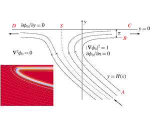
As described in detail in Cimpeanu & Moore (Reference Cimpeanu and Moore2018), the leading-order inner Helmholtz flow arising in the Wagner theory for symmetric droplet impact and its corresponding potential plane are depicted in figures 7–8 respectively. Adapting the solution of Wagner (Reference Wagner1932) for the problem of solid–liquid impact, the leading-order inner solution is given parametrically by

(5.15a,b ) $$\begin{eqnarray}\displaystyle \unicode[STIX]{x1D719}_{0}+\text{i}\hat{\unicode[STIX]{x1D713}}_{0}=\unicode[STIX]{x1D710}-\log \unicode[STIX]{x1D710}+1,\quad x+\text{i}y=-(1+\unicode[STIX]{x1D710}+4\sqrt{\unicode[STIX]{x1D710}}+\log \unicode[STIX]{x1D710}), & & \displaystyle\end{eqnarray}$$

where the fluid lies in $\text{Im}(\unicode[STIX]{x1D710})>0$ , the free surface lies along $\unicode[STIX]{x1D710}=a$ where $a$ is real and negative and the branch cuts are taken along the negative real axis. In particular, the free-surface profile is given parametrically by

(5.16a,b ) $$\begin{eqnarray}\displaystyle x(a)=-1-a-\log (-a),\quad y(a)=-\unicode[STIX]{x03C0}-4\sqrt{-a}, & & \displaystyle\end{eqnarray}$$

so that arc length along the free surface and its curvature are given by

(5.17a,b ) $$\begin{eqnarray}\displaystyle & \displaystyle s=1+a-\log (-a),\quad \unicode[STIX]{x1D705}=\frac{\sqrt{-a}}{(1-a)^{2}}, & \displaystyle\end{eqnarray}$$

where we note that $s\in (-\infty ,\infty )$ . Finally, we see that

(5.18) $$\begin{eqnarray}\displaystyle \tilde{w}^{\ast }=-2\unicode[STIX]{x03C0}+4\text{arctan}(\sqrt{-a}). & & \displaystyle\end{eqnarray}$$

Figure 7.

The (suitably scaled) leading-order inner problem according to Wagner theory for a droplet–droplet impact at small times. The dashed line indicates a dividing streamline that terminates at a relative stagnation point on the body at S. In a frame moving with the turnover points, the problem is a Helmholtz flow.

Figure 8.

The potential plane corresponding to the Helmholtz flow depicted in figure 7.

The map from the Wagner potential plane to the strip ${\mathcal{Z}}$ is given by

(5.19) $$\begin{eqnarray}\displaystyle \unicode[STIX]{x1D719}_{0}+\text{i}\unicode[STIX]{x1D713}_{0}=\text{e}^{\unicode[STIX]{x03C0}\unicode[STIX]{x1D701}}-\unicode[STIX]{x03C0}\unicode[STIX]{x1D701}+1, & & \displaystyle\end{eqnarray}$$

where, on the free surface, we can write $a=-\text{e}^{\unicode[STIX]{x03C0}\unicode[STIX]{x1D709}}$ to give

(5.20) $$\begin{eqnarray}\displaystyle s=\unicode[STIX]{x1D712}(\unicode[STIX]{x1D709})=-\unicode[STIX]{x03C0}\unicode[STIX]{x1D709}-\text{e}^{\unicode[STIX]{x03C0}\unicode[STIX]{x1D709}}+1. & & \displaystyle\end{eqnarray}$$

Note that $\unicode[STIX]{x1D709}=\infty$ corresponds to $s=-\infty$ and $\unicode[STIX]{x1D709}=-\infty$ corresponds to $s=\infty$ . Thus,

(5.21a,b ) $$\begin{eqnarray}\displaystyle & \displaystyle f(\unicode[STIX]{x1D709})=\unicode[STIX]{x1D712}^{\prime }(\unicode[STIX]{x1D709})\left.\frac{\unicode[STIX]{x2202}\unicode[STIX]{x1D719}_{1}}{\unicode[STIX]{x2202}s}\right|_{s=\unicode[STIX]{x1D712}(\unicode[STIX]{x1D709})},\quad g(\unicode[STIX]{x1D709})=\unicode[STIX]{x1D712}^{\prime }(\unicode[STIX]{x1D709})\left.\frac{\unicode[STIX]{x2202}\unicode[STIX]{x1D719}_{1}}{\unicode[STIX]{x2202}n}\right|_{s=\unicode[STIX]{x1D712}(\unicode[STIX]{x1D709})}, & \displaystyle\end{eqnarray}$$

and hence (4.10) gives

(5.22) $$\begin{eqnarray}\displaystyle & \displaystyle \unicode[STIX]{x1D712}^{\prime }(\unicode[STIX]{x1D709})\left.\frac{\unicode[STIX]{x2202}\unicode[STIX]{x1D719}_{1}}{\unicode[STIX]{x2202}n}\right|_{s=\unicode[STIX]{x1D712}(\unicode[STIX]{x1D709})}+\frac{1}{2}\unicode[STIX]{x2A0D}_{-\infty }^{\infty }\unicode[STIX]{x1D712}^{\prime }(t)\left.\frac{\unicode[STIX]{x2202}\unicode[STIX]{x1D719}_{1}}{\unicode[STIX]{x2202}s}\right|_{s=\unicode[STIX]{x1D712}(t)}\text{cosech}\left(\frac{\unicode[STIX]{x03C0}(\unicode[STIX]{x1D709}-t)}{2}\right)\,\text{d}t=0. & \displaystyle\end{eqnarray}$$

Now, recalling (3.16) and letting

(5.23a-c ) $$\begin{eqnarray}\displaystyle {h\unicode[STIX]{x0030A}}(\unicode[STIX]{x1D709})=\tilde{h}_{0}(s(\unicode[STIX]{x1D709})),\quad {\unicode[STIX]{x1D705}\unicode[STIX]{x0030A}}(\unicode[STIX]{x1D709})=\unicode[STIX]{x1D705}(s(\unicode[STIX]{x1D709})),\quad {w\unicode[STIX]{x0030A}}^{\ast }(\unicode[STIX]{x1D709})=\tilde{w}^{\ast }(s(\unicode[STIX]{x1D709})), & & \displaystyle\end{eqnarray}$$

we see that

(5.24) $$\begin{eqnarray}\frac{\text{d}{h\unicode[STIX]{x0030A}}}{\text{d}\unicode[STIX]{x1D709}}+\frac{1}{2}\unicode[STIX]{x2A0D}_{-\infty }^{\infty }\unicode[STIX]{x1D712}^{\prime }(t){\unicode[STIX]{x1D705}\unicode[STIX]{x0030A}}(t)\text{cosech}\left(\frac{\unicode[STIX]{x03C0}}{2}(\unicode[STIX]{x1D709}-t)\right)({h\unicode[STIX]{x0030A}}(t)-2{w\unicode[STIX]{x0030A}}^{\ast }(t))\,\text{d}t=-2\unicode[STIX]{x1D712}^{\prime }(\unicode[STIX]{x1D709}){\unicode[STIX]{x1D705}\unicode[STIX]{x0030A}}(\unicode[STIX]{x1D709}).\end{eqnarray}$$

As with (5.11), if we integrate (5.24) over all $\unicode[STIX]{x1D709}$ , then assuming the integrand satisfies a Hölder condition, we can reverse the order of integration, and, after returning to arc length as a variable, we deduce that

(5.25) $$\begin{eqnarray}\displaystyle & \displaystyle \tilde{h}_{0}(\infty )=\tilde{h}_{0}(-\infty )-2\int _{-\infty }^{\infty }\unicode[STIX]{x1D705}(s)\,\text{d}s=\tilde{h}_{0}(-\infty )-2\unicode[STIX]{x03C0}. & \displaystyle\end{eqnarray}$$

Thus, the ratio of the perturbation to the Wagner free surface upstream to that downstream is given by

(5.26) $$\begin{eqnarray}\displaystyle & \displaystyle \frac{(H+\unicode[STIX]{x1D700}^{2}\tilde{h}_{0})(\infty )}{(H+\unicode[STIX]{x1D700}^{2}\tilde{h}_{0})(-\infty )}=1+\frac{2\unicode[STIX]{x03C0}}{Re}+o\left(\frac{1}{Re}\right). & \displaystyle\end{eqnarray}$$

We can also solve (5.24) numerically by collocation. Firstly, note that

(5.27) $$\begin{eqnarray}\displaystyle & \displaystyle \unicode[STIX]{x1D712}^{\prime }(\unicode[STIX]{x1D709}){\unicode[STIX]{x1D705}\unicode[STIX]{x0030A}}(\unicode[STIX]{x1D709})=-\frac{\unicode[STIX]{x03C0}}{2}\text{sech}\frac{\unicode[STIX]{x03C0}\unicode[STIX]{x1D709}}{2}. & \displaystyle\end{eqnarray}$$

Thus, if we set

(5.28a-c ) $$\begin{eqnarray}\displaystyle \unicode[STIX]{x1D709}=\frac{-2\hat{\unicode[STIX]{x1D709}}}{\unicode[STIX]{x03C0}},\quad t=\frac{-2\hat{t}}{\unicode[STIX]{x03C0}},\quad {\hat{h}}(\hat{\unicode[STIX]{x1D709}})={h\unicode[STIX]{x0030A}}(\unicode[STIX]{x1D709})-2{w\unicode[STIX]{x0030A}}^{\ast }(\unicode[STIX]{x1D709}), & & \displaystyle\end{eqnarray}$$

we deduce that

(5.29) $$\begin{eqnarray}\displaystyle & \displaystyle \frac{\text{d}{\hat{h}}}{\text{d}\hat{\unicode[STIX]{x1D709}}}-\frac{1}{\unicode[STIX]{x03C0}}\unicode[STIX]{x2A0D}_{-\infty }^{\infty }\frac{{\hat{h}}(\hat{t})}{\cosh \hat{t}\sinh (\hat{\unicode[STIX]{x1D709}}-\hat{t})}\,\text{d}\hat{t}=\frac{2}{\cosh \hat{\unicode[STIX]{x1D709}}}, & \displaystyle\end{eqnarray}$$

which is remarkably similar to (5.11). As in (5.12)–(5.13), a far-field analysis of (5.29) shows us that

(5.30) $$\begin{eqnarray}\displaystyle & \displaystyle {\hat{h}}(\hat{\unicode[STIX]{x1D709}})\sim 4\left(1-\frac{1}{\unicode[STIX]{x03C0}}\int _{-\infty }^{\infty }\frac{{\hat{h}}(\hat{t})}{1+\text{e}^{2\hat{t}}}\,\text{d}\hat{t}\right)\text{e}^{\hat{\unicode[STIX]{x1D709}}}\quad \text{as }\unicode[STIX]{x1D709}\rightarrow -\infty , & \displaystyle\end{eqnarray}$$

(5.31) $$\begin{eqnarray}\displaystyle & \displaystyle {\hat{h}}(\hat{\unicode[STIX]{x1D709}})\sim 2\unicode[STIX]{x03C0}-8\hat{\unicode[STIX]{x1D709}}\text{e}^{-\hat{\unicode[STIX]{x1D709}}}-4\left(3+\frac{1}{\unicode[STIX]{x03C0}}\int _{-\infty }^{\infty }\frac{{\hat{h}}(\hat{t})-2\unicode[STIX]{x03C0}}{1+\text{e}^{-2\hat{t}}}\,\text{d}\hat{t}\right)\text{e}^{-\hat{\unicode[STIX]{x1D709}}}\quad \text{as }\hat{\unicode[STIX]{x1D709}}\rightarrow \infty . & \displaystyle\end{eqnarray}$$

Truncating the $\hat{\unicode[STIX]{x1D709}}$ -domain and utilising these far-field forms as previously, we can solve for ${\hat{h}}(\hat{\unicode[STIX]{x1D709}})$ numerically.

Figure 9.

The viscous correction to the free-surface location, $\tilde{h}_{0}(s)$ , for the Wagner jet root. Downstream as $s\rightarrow \infty$ , one can see the perturbation approaching the predicted value of $-2\unicode[STIX]{x03C0}$ , while upstream we see inverse square-root decay back into the bulk (the outer Wagner region), which we display in further detail in the inset, where the dashed line indicates square-root decay.

Returning to original variables, we plot the leading-order viscous correction $\tilde{h}_{0}(s)$ as a function of arc length in figure 9. The perturbation is again not monotonic in arc length near the point of maximum curvature in the inviscid problem ( $s=1.77$ ), although in this case we now see that the maximum normal shift from the Helmholtz solution is no longer far downstream, where we approach $-2\unicode[STIX]{x03C0}$ as predicted by (5.26). Moreover, we see much slower decay upstream as we move out of the Wagner jet root back into the outer region. The perturbation decays like $1/\sqrt{-s}$ as $s\rightarrow -\infty$ , which is expected when one considers the far field of the eigensolutions for the Laplace problem depicted in figure 7.

There are significant difficulties in reaching good quantitative agreement between the direct numerical simulation results and the asymptotic theory. Setting up a finite computational domain that is sufficiently large to appropriately incorporate the analytically derived far-field conditions requires length scales of at least $O(10^{2})$ . At the same time, as hinted in (5.26), the target solutions would differ by $O(Re^{-1})$ , which leads to a multi-scale environment spanning at least six orders of magnitude in a highly sensitive set-up. Furthermore, there are intrinsic subtleties connected to the construction of suitable boundary conditions in the gas, as well as immediately adjacent stable outflow boundary conditions in a non-trivially evolving flow. Ultimately we anticipate that the presence of surface tension effects, solving for the full Navier–Stokes solutions in both liquid and gas phases, as well as any discretisation errors in general would all lead to minor discrepancies at the level of the solution comparison. A representative result is illustrated on the left-hand side of figure 10, wherein an inset is used to indicate the accuracy of the comparison near the turnover region. As dictated by the scalings (3.3), we consider morphological features of interest at $O(1/Re)$ , thus making the set-up a very challenging one. Therefore even qualitative flow properties are very difficult to obtain and would in themselves contribute to a successful and informative study. We display such qualitative results in figure 10(b). In order to be consistent with the analytical formulation, the data extracted from the DNS have been shifted horizontally to fix the turnover point at $x=0$ and vertically to align with the jet far downstream. We have then calculated the normal distance between the inviscid free-surface profile and the simulation data. We see remarkably good qualitative agreement in the perturbation profile when comparing with figure (9), in particular capturing the square root decay upstream and the non-monotonic behaviour in the profile downstream of $s=0$ .

Figure 10.

(a) A typical comparison between the analytically predicted shape of the interface (dashed line), alongside a profile extracted from the direct numerical simulations (continuous line). The highlighted inset focuses on the discrepancies found near the turnover point. (b) The normal distance between the free-surface location as found via direct numerical simulation of the full Navier–Stokes problem and the inviscid prediction of Wagner theory. As elaborated upon in the text, we only concentrate on qualitative rather than quantitative comparisons between the analytical prediction and the results of the full simulations, but we see clear evidence of the shape of the viscous perturbation predicted by (5.29) and displayed in figure 9.

Figure 11.

Vorticity produced by the curved free boundary in the Wagner jet-root problem. The DNS results for the vorticity distribution in: (a) both the liquid and air phases; (b) the liquid phase only. The simulations use $Re=4000$ and $We=10\,000$ and we have included streamlines (in white) and chosen the colour bar scale to aid the visualisation. (c) Magnitude of the leading-order vorticity as predicted by the analytical solution. Both the numerical and analytical results show that the boundary layer thickens downstream of the turnover point, as predicted by (5.26).

Finally, we consider the vorticity in the jet-root problem. The vorticity is now given by

(5.32) $$\begin{eqnarray}\displaystyle & \displaystyle \unicode[STIX]{x1D74E}_{0}=-\frac{\unicode[STIX]{x2202}\tilde{w}_{0}}{\unicode[STIX]{x2202}{\tilde{n}}}\boldsymbol{k}, & \displaystyle\end{eqnarray}$$

where the change in sign from (5.14) comes from the change in chirality of the coordinate system.

We display the analytical prediction for the leading-order vorticity magnitude in figure 11(c). Similarly to the symmetric jets example and consistent with (5.26), we see that the boundary layer is thicker downstream of the turnover point ( $s=0$ ). A similar picture is seen from the vorticity data extracted from the DNS, as shown for the liquid phase in figure 11(b). As alluded to previously, although we can only really expect qualitative comparisons between the full numerical simulations and the analytical predictions, the minimum value of the vorticity in the numerical solution is $-0.62$ , which is not too dissimilar to the analytical prediction, which is approximately $-0.6$ (cf. figure 11 c). As with the symmetric jet case, we see in figure 11(a) that vorticity in the air is again larger than that in the liquid, although still of a similar order of magnitude.

Noticeably, in both the analytical predictions and the DNS results, there is no singularity in the boundary layer in this regime, and the conclusion reached in Batchelor (Reference Batchelor1967) and Moore et al. (Reference Moore, Ockendon, Ockendon and Oliver2014) still holds, namely that we require $\unicode[STIX]{x1D705}=O(Re)$ somewhere on the free surface for the vorticity to be shed into the inviscid bulk.