INTRODUCTION
In all European countries, before a new crop cultivar is released to the market, government authorities usually require cultivar (genotype) evaluation in official registration trials to assess its value for cultivation and use (VCU). Usually, the series of VCU trials extends over 2 or 3 years and many locations. In Croatia, the authority responsible for cultivar registration is the Institute for Seeds and Seedlings, evaluating 50 different crops at several locations evenly distributed across the individual crop's typical growing region in Croatia. The number of genotypes entering the first trial year ranges from just a few to more than 70 depending on the crop. On average, only 0·48 of the genotypes under evaluation are eventually released.
In multi-environment VCU trials, the genetic value of new genotypes is hidden by variation caused by genotype by environment interaction effects. This can be investigated by considering variance component estimates. Based on the analysis of the relative magnitude of the variance components, it is possible to classify and select superior plant material more precisely by determining how much each variance component contributes to the total phenotypic variance. Talbot (Reference Talbot1984, Reference Talbot1993); Moro et al. (Reference Moro, Alonso and Rodriguez1989); Laidig et al. (Reference Laidig, Drobek and Meyer2008) and Meyer et al. (Reference Meyer, Laidig and Drobek2011) analysed variance component estimates for various crops in the UK, Spain and Germany, explaining the nature of variation measured by the different components of variance and highlighting environmental variance components as a dominant part of total phenotypic variation for yield in all crops.
Recently, the genetic aspects of VCU trials have been analysed using the mixed model methodology in Canada (Yan & Rajcan Reference Yan and Rajcan2003), the UK (Smith et al. Reference Smith, Cullis and Thompson2005; Mackay et al. Reference Mackay, Horwell, Garner, White, Mckee and Philpott2011) and Germany (Piepho et al. Reference Piepho, Mohring, Melchinger and Buchse2008), due to highly unbalanced data sets with a large fraction of empty cells in the year × location × genotype three-way table. Typically, unbalanced variety trials data are frequently analysed by a mixed model procedure utilizing the restricted maximum-likelihood method (REML; Patterson Reference Patterson, Kempton, Fox and Cerezo1997).
Value for cultivation and use testing includes scoring for several economically important traits, but it is focused on the analysis of yield potential of new cultivars possibly translated into farm production in the near future. Yield predictions from the VCU trials are constantly higher than farm yields even if growing conditions are the same. When yields of VCU trials are compared with average on-farm yields for the given year, they must be assumed as ‘potential yields’, and yield gap between VCU trials and on-farm production may point to specificities of average yields obtained in large-scale growing conditions in a country.
Although there have been several studies of variance components in VCU trials in Western Europe and gaps between VCU trial yields and on-farm yields, no such study has been done in Eastern Europe where specific (un)favourable growing conditions might take place. The objectives of the present study were to describe the structure of crop-specific variance components and typical differences between crops for yield based on Croatian VCU results over the period from 2001 to 2010 and to compare the yield trends in the trials with national on-farm yields looking at relative yield gaps.
MATERIALS AND METHODS
Yield data from official Croatian variety trials assessing VCU of seven crops for the period 2001–10 were used in the present study. All trials were set as randomized complete block designs with four replicates and were machine-planted. Plot sizes were 10 m2 for winter crops (wheat, barley and oilseed rape), 11·2 m2 for maize and sunflower and 8 m2 for sugar beet. Grain yield, i.e. wheat, barley and maize, were standardized to 14% moisture, whereas oilseed rape and sunflower were standardized to 9% moisture. Standard cultural practices (fertilization, weed, pest and disease control) for specific crops were used before and during crop growing.
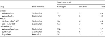
The seven crop data sets were classified into four groups: cereals, maize, oilseed crops and sugar beet (Table 1). The number of genotypes included all entries in all trials: controls, the genotypes entering the first trial year, genotypes subsequently withdrawn by breeders, as well as the genotypes (cultivars) finally released. The trials were equally distributed across the individual crop's typical growing region of the continental, northern part of Croatia including 5–7 sites, thus making a total of 37–49 trials per crop in the 10-year period.
Description of Croatian official variety trials in seven different crops evaluated in the period 2001–10

The data sets were both non-orthogonal and unbalanced due to ever-changing genotype sets, caused by a number of genotypes leaving or entering the trials from one year to another. Furthermore, even the set of sites was subject to some minor changes. Pre-processing of the data was done by analysing separately each of the 294 included trials to check for recording errors and outliers in order to avoid biased results. This step was carried out by running individual analyses of variance using the PLABSTAT program package (Utz Reference Utz1995).
The main analysis reported here was based on mean values, following the general model (1):
 $$y_{ijk} = \mu + G_i + L_j + Y_k + {\rm GL}_{ij} + {\rm GY}_{ik} + {\rm LY}_{\,jk} + e_{ijk} $$
where y ijk is the mean yield of the ith genotype in the jth location and the kth year, μ is the overall mean, G i is the main effect of ith genotype, L j is the main effect of jth location, Y k is the main effect of kth year, GL ij is the interaction of ith genotype with jth location, GY ik is the interaction of ith genotype with kth year, LY jk is the interaction of jth location with kth year and e ijk is the residual representing the confounded effects of genotype × location × year (GLY) interaction and experimental error. All effects except the grand mean are assumed to be random, with zero mean and normally distributed variances. The G, L, Y, GL, GY, LY and the residual variance components were estimated using the REML method implemented in lmer function from the R package lme4 (Bates et al. Reference Bates, Maechler, Bolker, Walker, Christensen, Singmann, Dai, Grothendieck and Green2012). Since the size of estimated variance components is related to the mean performance of individual crops (as reported by Talbot Reference Talbot1984), the effects were also presented as coefficients of variation, i.e. square roots of the variance component expressed as a percentage of the mean yield (Talbot Reference Talbot1993) in order to enable comparability between crops, and with results of other authors.
Further, yield gaps between on-farm and VCU trials were inspected by regressing annual mean yields from both sources on the 10-year trial period. The estimates of the gap size and tests for the heterogeneity of the regression lines (i.e. narrowing or widening of the gaps) were obtained by carrying out the analysis of covariance following the model (2), using the basic R package (R Core Team 2015):
 $$y_{ij} = \mu + S_j + b_i x_{ij} $$
where y ij is the mean yield from ith source and jth year, μ is the overall mean, S j the effect of the ith yield source (on-farm or variety trials), β i regression coefficient for the ith source, and x ij covariate (year). The contrast between two levels of the effect of source at a certain year provides an estimate of the gap size, while the interaction term (‘source:year’ in R syntax) is used to test for the inequality of slopes (thus, narrowing or widening of the gaps). Average annual on-farm yield data in Croatia were obtained from the national census (Croatian Bureau of Statistics 2016).
RESULTS
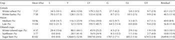
Mean yields across the crops were similar within a respective crop group (Table 2): about 7·5 t/ha in cereals, >10·0 t/ha in maize and about 4·0 t/ha for oilseed crops. In the groups of cereals and maize, the greatest variance components were from the location × year (LY) interaction, whereas in oilseed crops and sugar beet, the greatest variance components were due to year main effect (Y). On the other hand, genotype × location interaction (GL) was the smallest among the estimated variance components in cereals, maize and winter oilseed rape, while the location main effect (L) was negligible in sunflower and sugar beet. The genotype effect (G) was relatively small in winter barley and winter oilseed rape, explaining only 2·1 and 2·3% of the total yield variation respectively, whereas in sunflower and late maize G explained 12·2 and 13·4% of the total yield variation, respectively.
Genotypic, environmental and genotypic by environmental components of variance for yield of crops from official Croatian variety trials in the period 2001–10

L, location; Y, year; LY, location × year; G, genotype; GL, genotype × location; GY, Genotype × year.
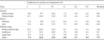
The coefficients of variation of components presented in Table 3 were the greatest for the environmental coefficients of LY, Y and L as well as of the residual. On average across all crops, the coefficient of LY was the greatest at 13·4%, and between 12 and 19% in cereals and maize. Variability of Y was dominant in oilseed crops and sugar beet. On average, coefficient of G was 6%, ranging from 3·9 to 7·6. The coefficient for the residual was larger than the values of G coefficients in cereals, oilseed crops and sugar beet.
Coefficients of variation for yield of crops from official Croatian variety trials in the period 2001–10

L, location; Y, year; LY, location × year; G, genotype; GL, genotype × location; GY, Genotype × year.
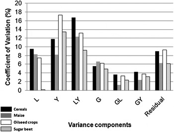
The average coefficients of variation for each of the four crop groups also showed that the greatest coefficients were those for environmental variation of LY and Y (Fig. 1); they are followed by the residual, which is only slightly greater than the third environmental component, L. These coefficients showed that cereals and oilseed crops responded particularly strongly to varying annual changes. Genotypic variation did not differ considerably among the four crop groups, while the smallest coefficients were observed for the GL interaction.
Average coefficient of genotypic, environmental, genotypic by environmental interactions variation for groups of crops in the period 2001–10.

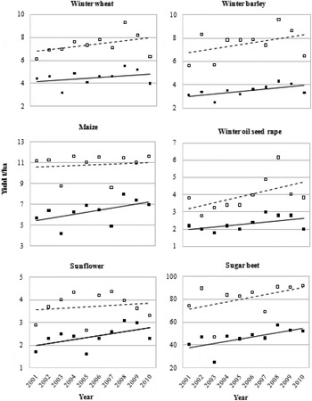
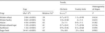
As expected, on-farm yields were considerably lower than VCU yields (Fig. 2). The smallest relative gap for year 2005 was estimated for sunflower, the greatest for winter barley, and all the gap estimates were significant at P < 0·001 (Table 4). In all cases, the trends were positive; however, the gaps seemed to be narrowing/widening with years and there was no statistical proof that would support this kind of conclusion for all of the investigated crops.
Trends of on-farm and variety trial yield means of winter wheat, winter barley, maize, winter oilseed rape, sunflower and sugar beet in Croatia in the period 2001–10.

Gaps and trends of annual on-farm and variety trial yield means

* Estimate for year 2005.
† For gap equals zero.
‡ To the variety trials estimate for year 2005.
§ Regression of mean yields on 10-year trial.
DISCUSSION
There are two major concerns when dealing with large unbalanced data sets such as those generated by combining variety trials over longer periods. The first is the use of significant computational time and resources, the second is the presence of time trends resulting in biased estimates of both G and Y variance components. In dealing with this problem, Laidig et al. (Reference Laidig, Drobek and Meyer2008) used the strategy of splitting the data into overlapping 2–3-year periods and analysing each period separately. Besides using smaller data sets that are less computationally demanding, this approach also provides a simple solution for the problem of bias caused by time trends, that can also be resolved by using complex solutions thoroughly elaborated by Mackay et al. (Reference Mackay, Horwell, Garner, White, Mckee and Philpott2011). The original intention for the current work was to use the strategy of Laidig et al. (Reference Laidig, Drobek and Meyer2008), but after completing the analysis for one crop, it was realised that running the analysis for the complete 10-year data sets was quite feasible. Comparing the sizes of Croatian, German and UK data sets, there is a ratio of 5–6 : 1 in number of locations between the German and Croatian data sets (which reflects approximately the same ratio between the sizes of the two countries), and a similar ratio in number of years between UK and Croatian data sets. After completing the analysis for the first crop using both complete and divided data set, no substantial differences were noticed between 10-year data set estimates and 3-year data sets averages, and no time trends in G and Y variance components. Therefore, it was decided to use the strategy of analysing the 10-year data sets without the correction for time trends.
Using the model that implicitly confounds the GLY interaction term with the experimental error, it was not possible to estimate this part of the genotype by environment interaction directly. Nevertheless, it was decided not to make any approximation of the GLY interaction variance component, since the present study was not a standard genotype × environment interaction analysis and GLY interaction was not of particular interest.
The results of the present study demonstrated that the relative magnitude of the variance components were similar to those obtained by Talbot (Reference Talbot1984) and Meyer et al. (Reference Meyer, Laidig and Drobek2011). Moreover, coefficients of genotypic (G) variation were much greater than those obtained in the UK and Germany for only a few crops (winter wheat and maize). A similar pattern was observed for the dominant source of variability, LY, which in the present study was considerably greater for maize and cereals. The same is true for the greatest effect of Y in oilseed crops and sugar beet. However, some crop-specific patterns do not entirely emulate similar patterns in German and UK studies and require further investigation. Hybrid crops generally tend to be less stable, thus resulting in larger environmental components (L, Y and LY). This could be a possible explanation for inflation of environmental components in winter oilseed rape, due to a shift from conventional cultivars to hybrids as the preferred crop type. Relatively small L variation for sunflower and sugar beet can be explained by a much smaller growing area for these two crops, with all the trial locations situated in relative proximity. During the period investigated, two severe droughts occurred in Croatia (2003 and 2007), decreasing the yields of both groups of medium and late maize hybrids. The droughts had a stronger effect on the medium group and that could be a possible cause for their greater Y component. On the other hand, the same argument probably cannot be used to explain the relationships between groups for other components, because the late group is characterized by higher effects of L and G, while the between-group ratios for components G and GL are inverse, and the same is true for Y and GY. Nevertheless, despite the wider range of environments covered by the studies of Meyer et al. (Reference Meyer, Laidig and Drobek2011) in Germany, differences between variance component estimates from the two series (Germany and Croatia) are not large. This indicates that the combinations of year and location within Croatia, if sufficiently widely sampled, can provide as extreme variety responses as a geographically more dispersed set of VCU trials.
Crop groups of cereals, maize, oilseed crops and sugar beet were quite homogenous, generating similar estimates within a group. Moreover, except for environmental effects (L, Y and LY), the variability of all other effects including G and the residual did not differ considerably across the crop groups. Environmental effects including seasonal variation (Y and LY) were always dominant, but variable among the groups. Seasonal variations of Y and LY were notably larger than ‘static’ variation of L, revealing a pattern typical for most of Croatian VCU data. Comparable results were presented by Smith et al. (Reference Smith, Cullis and Gilmour2001) in Australia. However, Meyer et al. (Reference Meyer, Laidig and Drobek2011) showed that variation of L is relatively more important in German VCU trials, whereas variation of Y is rather heterogeneous across the crop groups.
Rather than modelling the gap trend directly, the present study was based on an alternative approach. The major reason for this was the poor performance of the gap trend model, regression of differences (Laidig et al. Reference Laidig, Piepho, Drobek and Meyer2014), characterized by extremely low values of R 2. Analysis of covariance was a valuable alternative, providing the test for heterogeneity of slopes as the indicator of gap narrowing/widening. Non-significant tests for all crops indicate that despite some non-parallelism of the lines observable in Fig. 2, the gaps can be considered as constant over the 10-year period. Thus, the estimates of the relative gap are given for the midpoint, the year 2005.
Altogether, there was an increase in both VCU and on-farm yields in all crops, with no stagnation or decline of on-farm yields as had been observed in Western Europe (Peltonen-Sainio et al. Reference Peltonen-Sainio, Jauhiainen and Laurila2009; Brisson et al. Reference Brisson, Gate, Gouache, Charmet, Oury and Huard2010). The greatest gap for investigated crops in Croatia was recorded in winter barley, where yield levels for farm harvests were markedly below VCU trial yields. For winter wheat, the yield gap of 39% is notably greater than those reported by Laidig et al. (Reference Laidig, Piepho, Drobek and Meyer2014) in Germany (27%) and by Fischer & Edmeades (Reference Fischer and Edmeades2010) in the UK (30%), indicating considerable differences in breeding and agronomic conditions between Western Europe and Croatia. Fischer et al. (Reference Fischer, Byerlee and Edmeades2014) suggested that a yield gap of 30% on farm level could be economically achievable, while Lobell et al. (Reference Lobell, Cassman and Field2009) set the target to 20% in developed agriculture. In the present study, even the smallest overall gap is above these limits, and only one of the annual gaps was found to be at the target of 20% (sunflower in 2009). Generally, the gaps were between 30 and 60%, indicating generally greater gaps than those in Western Europe. The greater gaps arguably occurred due to specific growing and economic conditions in Croatia and possibly in southeast Europe in general. An agronomic explanation could be based on inadequate cultural practices and crop management, a phenomenon frequently encountered in Southeastern Europe due to economic reasons (Sudarić et al. Reference Sudarić, Šimić and Vratarić2006; Hristov et al. Reference Hristov, Mladenov, Djurić, Kondić-Špika, Marjanović-Jeromela and Šimić2010), which resulted in choosing physiologically effective, but not necessarily high-yielding genotypes in large-scale production. Further analyses of the exploitable yield (van Ittersum et al. Reference Van Ittersum, Cassman, Grassini, Wolf, Tittonell and Hochman2013) could possibly elucidate the regional yield gap specificities in different crops.
The authors wish to thank an anonymous reviewer for the valuable comments, which helped to improve the overall quality of the paper.