1 Introduction
Large-scale motion of magnetized plasmas may lead to variation of the magnitude of the magnetic field and of the plasma density. In the collisionless limit these changes drive particle temperature anisotropies that may lead to various plasma instabilities (Gary Reference Gary1993). Here we consider a homogeneous collisionless magnetized plasma consisting of electrons and protons. In this case, the perpendicular electron temperature anisotropy (i.e. when the perpendicular temperature is larger than the parallel one) in plasmas may generate (at least) two electromagnetic instabilities: the whistler/electron cyclotron instability that drives the whistler waves with the most unstable modes at electron scales that are parallel propagating with respect to the ambient magnetic field (except at very low beta plasmas, where the most unstable mode shifts to oblique angles, cf. Gary, Liu & Winske Reference Gary, Liu and Winske2011) and the mirror mode with wave vectors oblique with respect to the ambient magnetic field. The mirror instability driven only by anisotropic electrons is sometimes called the field-swelling instability (cf. Basu & Coppi Reference Basu and Coppi1984; Migliuolo Reference Migliuolo1986). Similarly, the perpendicular proton temperature anisotropy may generate (at least) two electromagnetic instabilities: the (parallel) proton cyclotron and the (oblique) mirror instability. Near threshold the mirror instability has only one branch, the most unstable mode appears at scales much larger than the characteristic particle scales (inertial lengths and gyroradii) and at strongly oblique angles with respect to the ambient magnetic field and both the species contribute to its destabilization. Further away from threshold the most unstable modes get shorter length scales and less oblique angles and the mirror instability may have two separate maxima one at larger (proton) scales and one at shorter (electron) scales (Noreen et al. Reference Noreen, Yoon, López and Zaheer2017). When the most unstable mode appears on proton/electron scales the instability will be called the proton/electron mirror instability here. We note, however, that the distinction between the two (and the large-scale mirror instability) is somewhat arbitrary, similarly to the distinction between proton and electron (and large) scales. On the other hand, the spatial and temporal scales of fluctuations determine the properties of their interaction with particles.
Mirror mode waves/structures are observed in the solar wind, planetary magnetosheaths and plasma sheets (Winterhalter et al. Reference Winterhalter, Neugebauer, Goldstein, Smith, Tsurutani, Bame and Balogh1995; Joy et al. Reference Joy, Kivelson, Walker, Khurana, Russell and Paterson2006; Tsurutani et al. Reference Tsurutani, Lakhina, Verkhoglyadova, Echer, Guarnieri, Narita and Constantinescu2011; Enríquez-Rivera et al. Reference Enríquez-Rivera, Blanco-Cano, Russell, Jian, Luhmann, Simunac and Galvin2013). These structures are non-propagating and pressure balanced and have the form of magnetic enhancements/peaks or depressions/holes with scales larger than but comparable to ion gyroscales. Magnetic peaks are typically observed in the region that are unstable with respect to the mirror instability whereas magnetic holes are seen in the stable region (Soucek, Lucek & Dandouras Reference Soucek, Lucek and Dandouras2008; Génot et al. Reference Génot, Budnik, Hellinger, Passot, Belmont, Trávníček, Sulem, Lucek and Dandouras2009). Isolated magnetic holes with a wide range of scales are often observed in the solar wind and some of them are likely related to the mirror instability (Stevens & Kasper Reference Stevens and Kasper2007). Sub-ion-scale magnetic peaks (Yao et al. Reference Yao, Shi, Guo, Yao, Tian, Degeling, Sun, Liu, Wang and Zong2018) and holes (Ge et al. Reference Ge, McFadden, Raeder, Angelopoulos, Larson and Constantinescu2011; Yao et al. Reference Yao, Wang, Shi, Pitkänen, Hamrin, Yao, Li, Ji, De Spiegeleer and Xiao2017; Zhang et al. Reference Zhang, Artemyev, Angelopoulos and Horne2017) are also sometimes observed. These structures are possibly generated by the electron mirror instability. However, the competing whistler instability driven by the electron perpendicular temperature anisotropy generally dominates over the electron mirror instability (Gary & Karimabadi Reference Gary and Karimabadi2006) even for relatively large electron betas. It is therefore questionable if the electron mirror instability is a relevant process in the space plasma context, in particular, for generating sub-ion-scale magnetic holes; other mechanisms may generate such structures (Balikhin et al. Reference Balikhin, Sibeck, Runov and Walker2012; Sundberg, Burgess & Haynes Reference Sundberg, Burgess and Haynes2015). On the other hand, the linear predictions are usually obtained assuming bi-Maxwellian particle distribution functions whereas in reality the electron distributions observed in situ are very different from bi-Maxwellian ones and generally include an important population of non-thermal particles with a power-law-like distribution (Štverák et al. Reference Štverák, Maksimovic, Trávníček, Marsch, Fazakerley and Scime2009) that affect the linear plasma properties (Pierrard et al. Reference Pierrard, Lazar, Poedts, Štverák, Maksimovic and Trávnícek2016; Shaaban et al. Reference Shaaban, Lazar, Astfalk and Poedts2018). Furthermore, a competition between different instabilities has to be investigated at the nonlinear level. Here we use a two-dimensional (2-D) version of a full particle-in-cell (PIC) code starting from an initial condition where both the whistler and electron mirror instability are unstable to see their competition.
This paper is organized as follows: § 2 presents linear predictions for the two instabilities, § 3 describes the numerical code and presents the simulation results. The presented results are summarized and discussed in § 4.
2 Linear predictions
The condition for the mirror instability in a plasma consisting of an arbitrary set of species (denoted by the subscript
 $s$
) with bi-Maxwellian velocity distribution functions that are non-drifting with respect to each other can be given as
 $\unicode[STIX]{x1D6E4}>0$
where
 $$\begin{eqnarray}\displaystyle \unicode[STIX]{x1D6E4}=\mathop{\sum }_{s}\unicode[STIX]{x1D6FD}_{\bot s}\left(\frac{T_{\bot s}}{T_{\Vert s}}-1\right)-1-\frac{\displaystyle \left(\mathop{\sum }_{s}\unicode[STIX]{x1D70C}_{s}T_{\bot s}/T_{\Vert s}\right)^{2}}{\displaystyle 2\mathop{\sum }_{s}\unicode[STIX]{x1D70C}_{s}^{2}/\unicode[STIX]{x1D6FD}_{\Vert s}}, & & \displaystyle\end{eqnarray}$$
where
 $T_{\bot s}$
and
 $T_{\Vert s}$
denote the perpendicular and parallel particle temperatures, respectively,
 $\unicode[STIX]{x1D6FD}_{\bot s}$
and
 $\unicode[STIX]{x1D6FD}_{\Vert s}$
denote the perpendicular and parallel betas (ratios between the particle and magnetic pressures), respectively,
 $\unicode[STIX]{x1D70C}_{s}$
denotes the particle charge densities;
 $\sum _{s}$
denotes a sum over all species (cf. Stix Reference Stix1962; Hasegawa Reference Hasegawa1969; Hellinger Reference Hellinger2007); here we consider only protons and electrons with the subscripts
 $p$
and
 $e$
, respectively.
We start with a short analysis of the relationship between the proton and electron mirror instability far from threshold. First, we investigate the linear prediction for the mirror instability near threshold for
 $\unicode[STIX]{x1D6E4}=0.01$
(i.e. we keep the same distance from the threshold) and for constant total electron and proton betas,
 $\unicode[STIX]{x1D6FD}_{e}=\unicode[STIX]{x1D6FD}_{\Vert e}(1+2T_{\bot e}/T_{\Vert e})/3=1$
and
 $\unicode[STIX]{x1D6FD}_{p}=\unicode[STIX]{x1D6FD}_{\Vert p}(1+2T_{\bot p}/T_{\Vert p})/3=1$
, using a full linear Vlasov solver (Hellinger et al.
Reference Hellinger, Trávníček, Kasper and Lazarus2006). The system constrained by
 $\unicode[STIX]{x1D6E4}=1$
and
 $\unicode[STIX]{x1D6FD}_{e}=\unicode[STIX]{x1D6FD}_{p}=1$
gives a one-dimensional dependence of the maximum growth rate
 $\unicode[STIX]{x1D6FE}_{m}$
on the electron temperature anisotropy (
 $T_{\bot p}/T_{\Vert p}$
decreases while
 $T_{\bot e}/T_{\Vert e}$
increases to keep
 $\unicode[STIX]{x1D6E4}$
constant; the maximum of
 $T_{\bot e}/T_{\Vert e}$
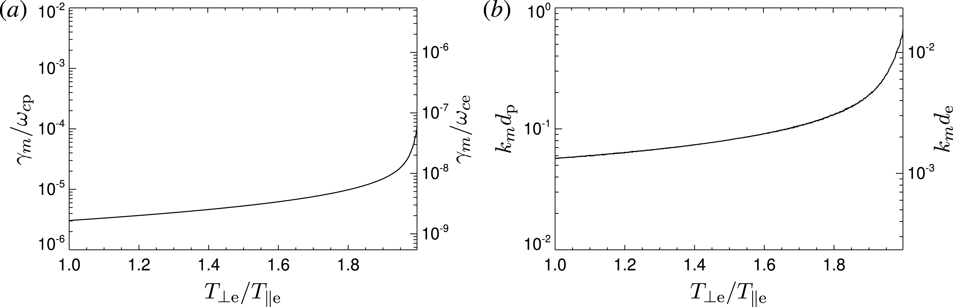
corresponds to isotropic protons and vice versa). The results of this calculation are shown in figure 1. This figure shows that the maximum growth rate
 $\unicode[STIX]{x1D6FE}_{m}$
is small fraction of the proton cyclotron frequency,
 $\unicode[STIX]{x1D714}_{cp}$
, and increases with the increasing electron temperature anisotropy. The wavelength of the most unstable mode
 $2\unicode[STIX]{x03C0}/k_{m}$
is relatively large with respect to the proton inertial length
 $d_{p}$
(here comparable to the proton gyroradius
 $\unicode[STIX]{x1D70C}_{p}$
) and increases with
 $T_{\bot e}/T_{\Vert e}$
and remains large with respect to the electron inertial length
 $d_{e}$
. These results indicate that even close to threshold the typical spatial temporal scales of the mirror mode are influenced by the particles with a dominant perpendicular temperature anisotropy.
(a) The maximum growth rate
 $\unicode[STIX]{x1D6FE}_{m}$
of the mirror instability (normalized to the proton cyclotron frequency
 $\unicode[STIX]{x1D714}_{cp}$
or to the electron one
 $\unicode[STIX]{x1D714}_{ce}$
) and (b) the wave vector of the most unstable mode
 $k_{m}$
(normalized to the proton inertial length
 $d_{p}$
or to the electron one
 $d_{e}$
) along a one-dimensional subspace of the four-dimensional space
 $(\unicode[STIX]{x1D6FD}_{\Vert p},T_{\bot p}/T_{\Vert p},\unicode[STIX]{x1D6FD}_{\Vert e},T_{\bot e}/T_{\Vert e})$
determined by the three conditions
 $\unicode[STIX]{x1D6E4}=0.01$
,
 $\unicode[STIX]{x1D6FD}_{e}=\unicode[STIX]{x1D6FD}_{p}=1$
(see the text). This subspace is parametrized by
 $T_{\bot e}/T_{\Vert e}$
.

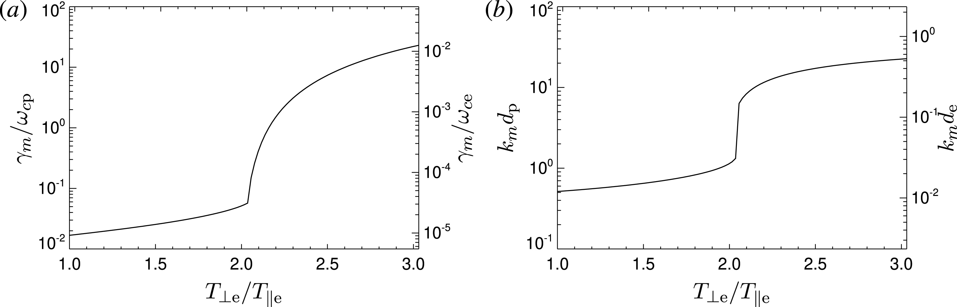
(a) The maximum growth rate
 $\unicode[STIX]{x1D6FE}_{m}$
of the electron/proton mirror instability and (b) the wave vector of the most unstable mode
 $k_{m}$
along a one-dimensional subspace of the four-dimensional space
 $(\unicode[STIX]{x1D6FD}_{\Vert p},T_{\bot p}/T_{\Vert p},\unicode[STIX]{x1D6FD}_{\Vert e},T_{\bot e}/T_{\Vert e})$
determined by the three conditions
 $\unicode[STIX]{x1D6E4}=1$
,
 $\unicode[STIX]{x1D6FD}_{e}=\unicode[STIX]{x1D6FD}_{p}=1$
(see the text). This subspace is parametrized by
 $T_{\bot e}/T_{\Vert e}$
.

The same analysis for
 $\unicode[STIX]{x1D6E4}=1$
, i.e. relatively far from threshold, is shown in figure 2. In the case, when the proton temperature anisotropy dominates,
 $\unicode[STIX]{x1D6FE}_{m}$
is a small fraction of
 $\unicode[STIX]{x1D714}_{cp}$
(with
 $k_{m}$
on proton scales) whereas when the electron temperature anisotropy becomes dominant, there is a rapid transition and
 $\unicode[STIX]{x1D6FE}_{m}$
is then rather a small fraction of the electron cyclotron frequency
 $\unicode[STIX]{x1D714}_{ce}$
(with
 $k_{m}$
on electron scales) and comparable to or larger than
 $\unicode[STIX]{x1D714}_{cp}$
. In the transition region there may exist two separate local maxima (Noreen et al.
Reference Noreen, Yoon, López and Zaheer2017). The behaviour seen in figure 2 is quite general, we observe similar properties for
 $\unicode[STIX]{x1D6FD}_{e}=\unicode[STIX]{x1D6FD}_{p}=10$
,
 $\unicode[STIX]{x1D6FD}_{e}=10$
and
 $\unicode[STIX]{x1D6FD}_{p}=1$
, and
 $\unicode[STIX]{x1D6FD}_{e}=1$
and
 $\unicode[STIX]{x1D6FD}_{p}=10$
while keeping
 $\unicode[STIX]{x1D6E4}=1$
. Henceforth, we assume that protons are isotropic and the perpendicular electron temperature anisotropy is only the only source of free energy for instabilities.
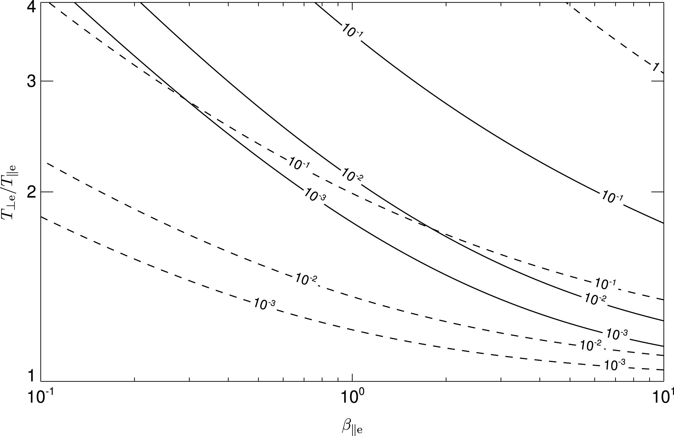
Figure 3 shows the maximum growth rate
 $\unicode[STIX]{x1D6FE}_{m}$
of (solid) the electron mirror and (dashed) the whistler instability as a function of the electron beta and the electron temperature anisotropy assuming bi-Maxwellian electrons and Maxwellian protons; the ratio between the electron plasma and cyclotron frequencies is assumed to be
 $\unicode[STIX]{x1D714}_{pe}/\unicode[STIX]{x1D714}_{ce}=100$
(relevant for the solar wind).
The comparison between the linear predictions for the whistler and mirror instabilities in figure 3 clearly confirms that the whistler instability is typically linearly dominant and one expects that the electron mirror instability is not generally very relevant (Gary & Karimabadi Reference Gary and Karimabadi2006). However, the linear predictions have limited applicability, it is necessary to take into account the nonlinear behaviour of the two instabilities.
3 Simulation results
To investigate nonlinear properties of the two instabilities and their competition we use a 2-D version of an explicit electromagnetic PIC code that employs the Darwin approximation (Decyk Reference Decyk2007; Schriver et al. Reference Schriver, Ashour-Abdalla, Coroniti, LeBoeuf, Decyk, Travnicek, Santolík, Winningham, Pickett and Goldstein2010). The Darwin PIC model neglects the transverse component of the displacement current (but keeps the longitudinal part) in the full set of Maxwell’s equations, which makes them radiation free, but leaves the whistler physics unaffected by its fully electromagnetic counterpart (Hewett Reference Hewett1985); the radiation-free Darwin approximation removes the demanding Courant–Friedrich–Levy condition for a time step given by the speed of light (Schriver et al. Reference Schriver, Ashour-Abdalla, Coroniti, LeBoeuf, Decyk, Travnicek, Santolík, Winningham, Pickett and Goldstein2010; Hellinger et al. Reference Hellinger, Trávníček, Decyk and Schriver2014). Consequently, the time step is set by the greater of the electron plasma frequency or the electron cyclotron frequency.
Here we use the real mass ratio
 $m_{p}/m_{e}=1836$
. For the frequency ratio we use
 $\unicode[STIX]{x1D714}_{pe}/\unicode[STIX]{x1D714}_{ce}=4$
in order to save the numerical resources (by reducing the ratio between the electron inertial length
 $d_{e}$
and the Debye length
 $\unicode[STIX]{x1D706}_{D}$
). Note that the linear prediction in figure 3 is calculated for
 $\unicode[STIX]{x1D714}_{pe}/\unicode[STIX]{x1D714}_{ce}=100$
; further linear analysis shows that the linear properties of the electron whistler and mirror instabilities depend only weakly on this ratio, a calculation analogous to figure 3 for
 $\unicode[STIX]{x1D714}_{pe}/\unicode[STIX]{x1D714}_{ce}=4$
gives results almost identical to that of figure 3.
The maximum growth rate
 $\unicode[STIX]{x1D6FE}_{m}$
of (solid) the mirror instability and (dashed) the electron whistler instability as a function of the electron beta and the electron temperature anisotropy. The solid and dashed contours are annotated by
 $\unicode[STIX]{x1D6FE}_{m}$
normalized to
 $\unicode[STIX]{x1D714}_{ce}$
.

The electrons have initially
 $\unicode[STIX]{x1D6FD}_{\Vert e}=10$
and
 $T_{\bot e}/T_{\Vert e}=1.52$
whereas the protons are initially isotropic with
 $T_{p}=T_{\Vert e}$
. The simulation box is chosen to be a 2-D grid
 $2048^{2}$
with the physical sizes
 ${\sim}1145^{2}d_{e}^{2}$
. The magnetic field is chosen to be along the
 $x$
-direction. There are 1024 macroparticles per cell for electrons and 512 macroparticles per cell for protons. The time step is
 $\unicode[STIX]{x0394}t=0.05\unicode[STIX]{x1D714}_{ce}^{-1}$
.
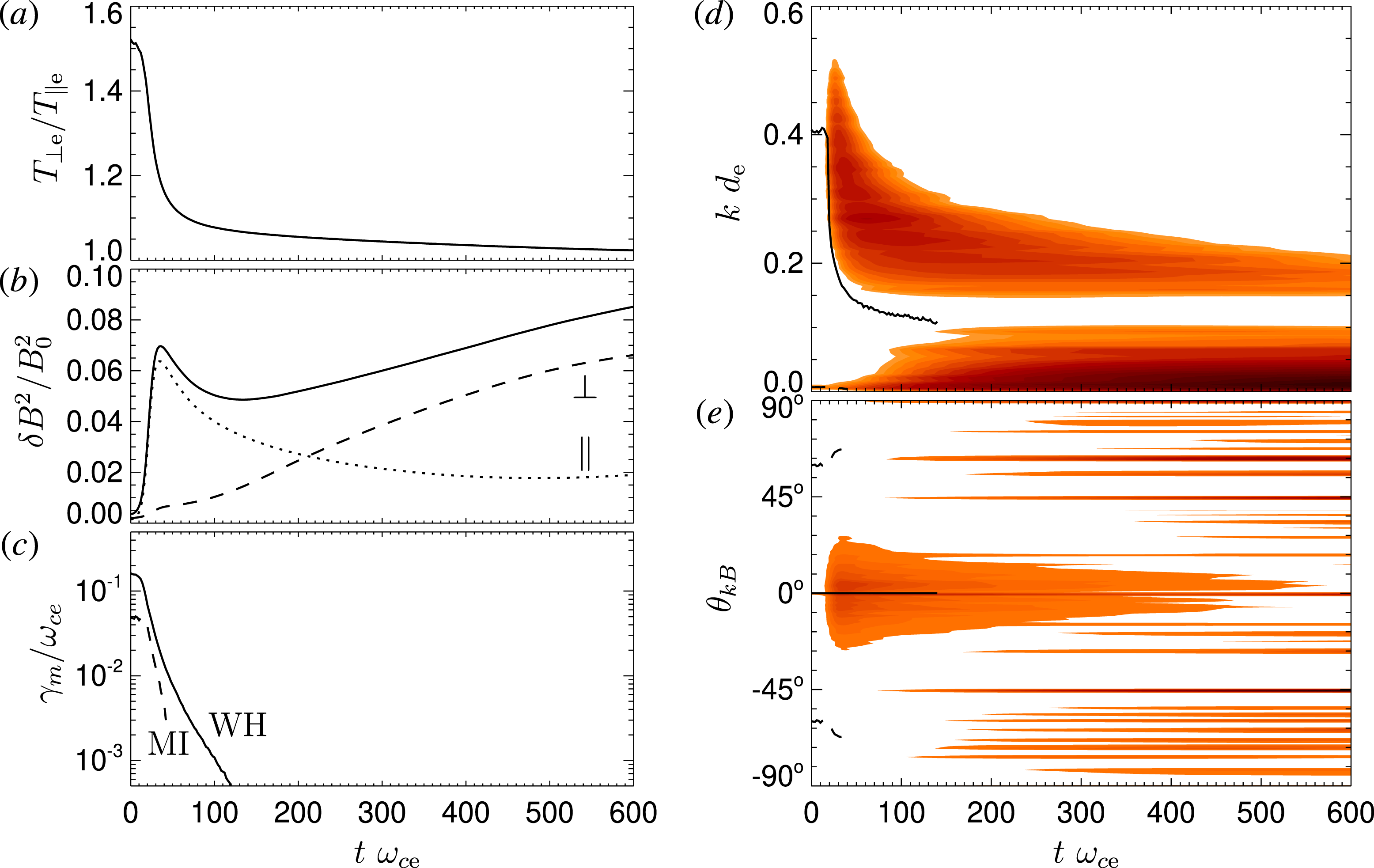
The time evolution of the system is shown in figure 4: figure 4(a) shows the evolution of the electron temperature anisotropy
 $T_{\bot e}/T_{\Vert e}$
. Figure 4(b) displays the total fluctuating magnetic field
 $\unicode[STIX]{x1D6FF}B^{2}/B_{0}^{2}$
(solid line) as a function of time; for comparison, the dotted and dashed curves display the fluctuating magnetic field with quasi-parallel (
 $\unicode[STIX]{x1D703}_{kB}\leqslant 45^{\circ }$
) and quasi-perpendicular (
 $\unicode[STIX]{x1D703}_{kB}>45^{\circ }$
) wave vectors, respectively. Figure 4(c) presents results of the linear analysis based on the instantaneous electron velocity distribution function (Hellinger & Trávníček Reference Hellinger and Trávníček2011; Hellinger et al.
Reference Hellinger, Trávníček, Decyk and Schriver2014), the maximum growth rate
 $\unicode[STIX]{x1D6FE}_{m}$
for the whistler (solid) and mirror (dashed) instabilities as functions of time. Figures 4(d) and 4(e) display colour scale plots of the fluctuating magnetic field
 $\unicode[STIX]{x1D6FF}B$
as a function of time and wave vector
 $k$
and as a function of time and propagation angle
 $\unicode[STIX]{x1D703}_{kB}$
, respectively. Solid and dashed lines (in d and e) show the properties (
 $k$
and
 $\unicode[STIX]{x1D703}_{kB}$
) of the most unstable mode for the whistler and mirror instability (see c), respectively.
(a–c) The electron temperature anisotropy
 $T_{\bot e}/T_{\Vert e}$
(a), the fluctuating magnetic field
 $\unicode[STIX]{x1D6FF}B^{2}/B_{0}^{2}$
(b) and the instantaneous maximum growth rate
 $\unicode[STIX]{x1D6FE}_{m}$
normalized to
 $\unicode[STIX]{x1D714}_{ce}$
(c) as functions of time. Dotted and dashed lines in (b) shows the fluctuating magnetic field with
 $\unicode[STIX]{x1D703}_{kB}\leqslant 30^{\circ }$
and
 $\unicode[STIX]{x1D703}_{kB}>30^{\circ }$
, respectively. (d,e) Colour scale plots of the fluctuating magnetic field
 $\unicode[STIX]{x1D6FF}B$
as a function of time and wave vector
 $k$
(d) and as a function of time and propagation angle
 $\unicode[STIX]{x1D703}_{kB}$
(e). Solid and dashed lines (in d and e) show the properties (
 $k$
and
 $\unicode[STIX]{x1D703}_{kB}$
) of the most unstable mode for the whistler and mirror instability (see c), respectively.

Figure 4 shows that the plasma system with anisotropic electrons generates mostly quasi-parallel (whistler) waves at electron scales that importantly reduce the electron temperature anisotropy. At the same time, at relatively large scales (and oblique propagation) other fluctuations appear. The amplitude of the whistler waves decreases after the saturation (at approximately
 $40/\unicode[STIX]{x1D714}_{ce}$
). The (quasi-)linear prediction based on the instantaneous electron distribution function indicate that the whistler mode is stabilized after
 $t\simeq 100/\unicode[STIX]{x1D714}_{ce}$
; the electron mirror instability is linearly stabilized earlier, after
 $t\simeq 50/\unicode[STIX]{x1D714}_{ce}$
. The evolution of whistler wave activity follows to some extent the quasi-linear prediction (solid lines on figure 4
d,e). The spectrum of magnetic fluctuations shifts to large scales after the saturation in agreement with the shift of the most unstable mode (and also the whole unstable region) to larger scales a short time before the saturation (the natural delay is owing to the fact the growth/damping rate gives just the relative rate of amplitude change). The initial decrease of the whistler wave activity seems to be related to the shift of the unstable region, some short-wavelength modes that reached important amplitudes become damped.
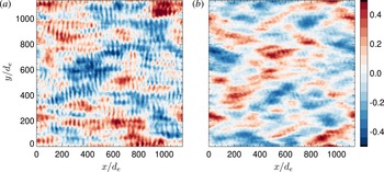
In contrast with the (quasi-)linear prediction, the simulation exhibits a continuous increase of fluctuations at oblique angles. These fluctuations have the form of coherent structures as seen in figure 5. This figure displays the spatial structure of the fluctuating magnetic field (
 $\unicode[STIX]{x1D6FF}B_{z}$
and
 $\unicode[STIX]{x1D6FF}B_{x}$
components) at end of the simulation. At this time the system is quasi-stationary, we do not observe big/qualitative changes during the period 500–
 $600\unicode[STIX]{x1D714}_{ce}^{-1}$
. Figure 5 shows that the electromagnetic fluctuations are composed of quasi-parallel (whistler) waves and oblique compressible structures. These structures are essentially non-propagating and exhibit a weak anti-correlation between
 $B_{x}$
and the electron density
 $n_{e}$
.
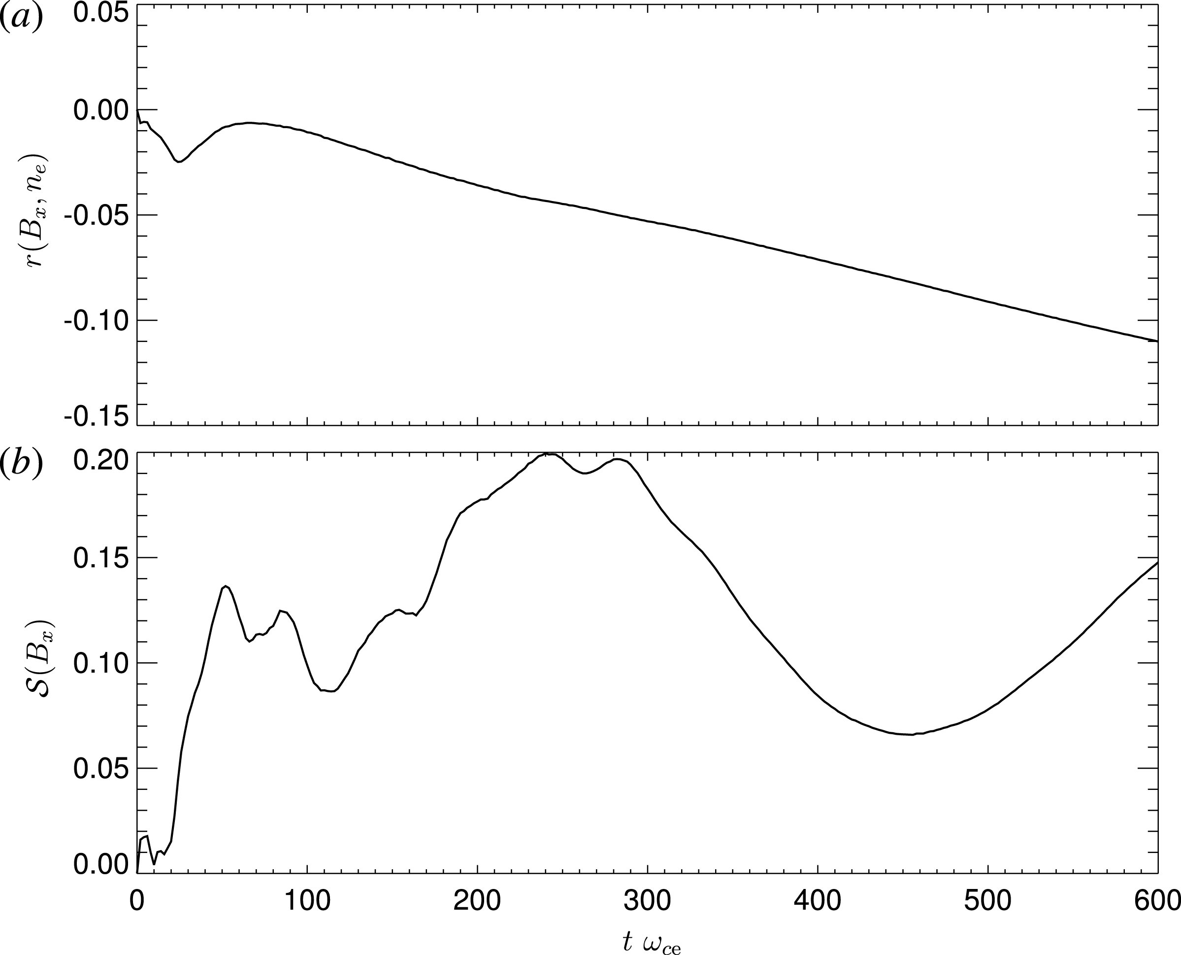
Figure 6 shows the evolution of the system, the correlation coefficient between the compressible magnetic component
 $B_{x}$
and the electron number density
 $r(B_{x},n_{e})$
and the skewness of
 $B_{x}$
 ${\mathcal{S}}(B_{x})$
as functions of time. The (sample) correlation coefficient of two discrete variables
 $x$
and
 $y$
is given by
 $$\begin{eqnarray}\displaystyle r(x,y)=\frac{\displaystyle \frac{1}{n}\mathop{\sum }_{i=1}^{n}(x_{i}-\bar{x})(y_{i}-\bar{y})}{\displaystyle \sqrt{\mathop{\sum }_{i=1}^{n}(x_{i}-\bar{x})^{2}}\sqrt{\mathop{\sum }_{i=1}^{n}(y_{i}-\bar{y})^{2}}}, & & \displaystyle\end{eqnarray}$$
where
 $\bar{x}=\sum _{i=1}^{n}x_{i}/n$
and
 $\bar{y}=\sum _{i=1}^{n}y_{i}/n$
are the mean values,
 $n$
is the number of grid points. The (sample) skewness of a discrete variable
 $x$
is given by
 $$\begin{eqnarray}\displaystyle {\mathcal{S}}(x)=\frac{\sqrt{n(n-1)}}{n-2}\frac{\displaystyle \frac{1}{n}\mathop{\sum }_{i=1}^{n}(x_{i}-\bar{x})^{3}}{\displaystyle \left[\frac{1}{n}\mathop{\sum }_{i=1}^{n}(x_{i}-\bar{x})^{2}\right]^{3/2}}. & & \displaystyle\end{eqnarray}$$
Colour scale plots of the fluctuating magnetic field (a)
 $\unicode[STIX]{x1D6FF}B_{z}$
and (b)
 $\unicode[STIX]{x1D6FF}B_{x}$
as a function of
 $x$
and
 $y$
at the end of the simulation.

Evolution of the system, (a) the correlation coefficient (solid) between the compressible magnetic component
 $B_{x}$
and the electron number density
 $r(B_{x},n_{e})$
, (b) and the skewness of
 $B_{x}$
 ${\mathcal{S}}(B_{x})$
as functions of time.

The compressible magnetic component
 $B_{x}$
is weakly anti-correlated with the electron density throughout the simulation; this anti-correlation becomes more pronounced at later times when the oblique fluctuations get stronger. This property is consistent with the linear as well as nonlinear expectation for the electron mirror instability. The distribution of values
 $B_{x}$
has a positive skewness throughout the simulation. It grows, oscillates, decreases for
 $300/\unicode[STIX]{x1D714}_{ce}\lesssim t\lesssim 450/\unicode[STIX]{x1D714}_{ce}$
, and grows again after
 $t\gtrsim 450/\unicode[STIX]{x1D714}_{ce}$
. This indicates that the coherent structures seen in the simulation (see figure 5) are rather magnetic enhancements (peaks/humps) (cf. Génot et al.
Reference Génot, Budnik, Hellinger, Passot, Belmont, Trávníček, Sulem, Lucek and Dandouras2009). We interpret the oblique fluctuations as nonlinear electron mirror structures.
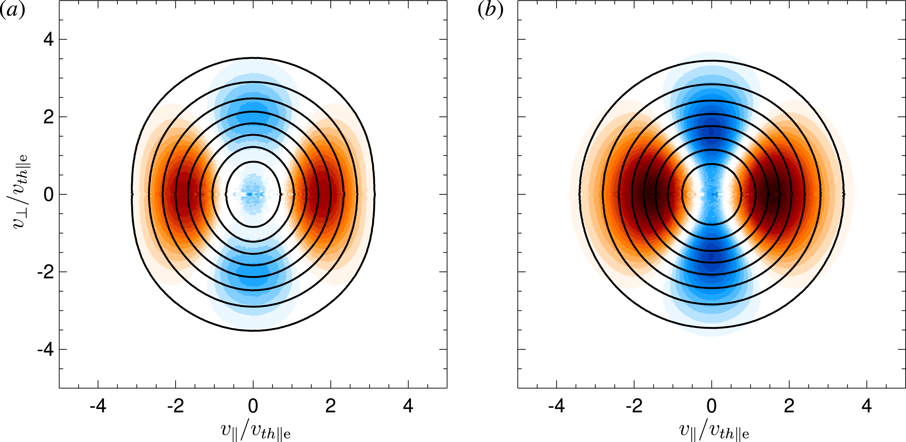
Electron velocity distribution functions shown as solid contours at (a)
 $t=36\unicode[STIX]{x1D714}_{ce}^{-1}$
and (b)
 $t=600\unicode[STIX]{x1D714}_{ce}^{-1}$
. The colour scale plots display the change of the distribution function
 $\unicode[STIX]{x1D6FF}f=f(t)-f(0)$
where shades of red (blue) denote positive (negative) values.

Finally, figure 7 shows the electron velocity distribution functions at the time of the saturation of the whistler instability (
 $t=36\unicode[STIX]{x1D714}_{ce}^{-1}$
) and at the end of the simulation (
 $t=600\unicode[STIX]{x1D714}_{ce}^{-1}$
). This figure suggests that around the whistler saturation the electron distribution function have a shape reminiscent of a quasi-linear cyclotron plateau (Kennel & Engelmann Reference Kennel and Engelmann1966). At later stages of the simulation, when the whistler activity decays and electron mirror structures become dominant, the electron velocity distribution function has a shape that is relatively close to a bi-Maxwellian one with a weak anisotropy (see figure 4). For the sake of completeness, we note that protons are essentially unaffected by the electron whistler and mirror modes, the relative change of their temperature is of the order of
 $10^{-4}$
during the simulation.
4 Discussion
In a proton–electron plasma the mirror instability may have the most unstable mode on proton or electron scales far from threshold. We investigated the linear prediction for one parameter case where we kept the same distance from the threshold and the same total betas for protons and electrons. The most unstable mode appears on proton scales roughly in the region where protons were more anisotropic then electrons and vice versa. How this linear prediction works in the four-dimensional space of proton and electron temperature anisotropies and (parallel) betas is an open problem beyond the scope of this paper; this behaviour is also affected by the presence of suprathermal populations (Shaaban et al.
Reference Shaaban, Lazar, Astfalk and Poedts2018). These results could also depend on the ratio
 $\unicode[STIX]{x1D714}_{pe}/\unicode[STIX]{x1D714}_{ce}$
but our results indicate that this dependence is weak.
The 2-D PIC simulation of a system initially unstable with respect to both the whistler and electron mirror instabilities shows that the linearly dominant whistler instability rapidly generates quasi-parallel whistler waves that reduce the electron temperature anisotropy. Meanwhile, the mirror modes slowly grow but are rapidly linearly stabilized owing to the dominant whistler instability. However, the mirror modes continue to grow and become dominant electromagnetic fluctuations in the form of coherent magnetic enhancements/peaks at electron scales. At the same time, the amplitude of whistler waves decreases probably partly owing to the presence of important electron mirror structures; on the other hand, similar decay is seen also without mirror modes for a relatively strong whistler instability (Kim, Hwang, Seough & Yoon Reference Kim, Hwang, Seough and Yoon2017).
A nonlinear growth of mirror structures that appears after the (quasi-)linear saturation was observed in a numerical simulation (in the hybrid, kinetic ion and fluid electron, approximation) for the proton mirror instability (Califano et al. Reference Califano, Hellinger, Kuznetsov, Passot, Sulem and Trávníček2008); in this case the proton mirror instability forms coherent structures in the form of magnetic peaks on proton scales. We expect that the formation of electron mirror structures seen in the full particle simulations is driven by a similar/analogous phenomenon. The nonlinear growth of the (proton) mirror structures is in agreement with the nonlinear dynamic model of Kuznetsov, Passot & Sulem (Reference Kuznetsov, Passot and Sulem2007b ,Reference Kuznetsov, Passot and Sulem a ) for the mirror instability near threshold, based on a reductive perturbative expansion of the Vlasov–Maxwell equations. This model extends the mirror dispersion relation by including the dominant nonlinear coupling whose effect is to reinforce the mirror instability. In the present case, the system is relatively far from threshold but the simulations results are qualitatively in agreement with this model. The basic disagreement between the model and simulations, seen also in the hybrid simulations, is that the model predicts formation of magnetic depression/holes whereas the simulations show formation of magnetic enhancements/peaks. This difference may be related to the flattening of the distribution function that may lead to a change of the nonlinear term (Hellinger et al. Reference Hellinger, Kuznetsov, Passot, Sulem and Trávníček2009).
The present results are based on one case with ad hoc parameters where the electron temperature anisotropy is quite strong so that both the modes are initially unstable. Consequently, the whistler instability has quite a fast initial maximum growth rate. This may require a fast anisotropization mechanism. On the other hand, in a more realistic case where the temperature anisotropy is continuously driven, for example by the plasma expansion/compression (Hellinger et al. Reference Hellinger, Trávníček, Mangeney and Grappin2003a ,Reference Hellinger, Trávníček, Mangeney and Grappin b ; Sironi & Narayan Reference Sironi and Narayan2015; Hellinger Reference Hellinger2017) or by the velocity shear (Kunz, Schekochihin & Stone Reference Kunz, Schekochihin and Stone2014; Riquelme, Quataert & Verscharen Reference Riquelme, Quataert and Verscharen2015), the dominant instability may not be efficient enough to arrest the anisotropy above threshold of the subordinate instability and the latter may be eventually destabilized and affect the system behaviour. Driven simulations of Trávníček et al. (Reference Trávníček, Hellinger, Taylor, Escoubet, Dandouras and Lucek2007) and Ahmadi, Germaschewski & Raeder (Reference Ahmadi, Germaschewski and Raeder2017) exhibit the formation of magnetic enhancements/peaks in the region unstable with respect to the proton mirror instability and a transformation of these peaks to magnetic holes as the system becomes more stable in agreement with in situ observations (Génot et al. Reference Génot, Broussillou, Budnik, Hellinger, Trávníček, Lucek and Dandouras2011). We expect a similar behaviour for the electron mirror instability, some of the observed sub-ion-scale magnetic holes (Ge et al. Reference Ge, McFadden, Raeder, Angelopoulos, Larson and Constantinescu2011; Yao et al. Reference Yao, Wang, Shi, Pitkänen, Hamrin, Yao, Li, Ji, De Spiegeleer and Xiao2017; Zhang et al. Reference Zhang, Artemyev, Angelopoulos and Horne2017) may be generated by an analogous process.
The presented simulation results have many limitations. We used a 2-D code. In the realistic three-dimensional case the oblique mirror modes have more degree of freedom and likely play a more important role (cf. Shoji et al. Reference Shoji, Omura, Tsurutani, Verkhoglyadova and Lembege2009). The limited number of particles per cell leads (and the large beta) leads to a non-negligible noise level that affect the initial level of fluctuation and, consequently, the nonlinear competition of different modes. Another problem is that at the end of the simulation the amplitude of magnetic fluctuations is still growing. The growth is, however, rather weak and we do not expect that the evolution would change significantly at later times. Also, we investigated a spatially homogeneous case. The evolution of the system may be importantly influenced by the presence of important turbulent fluctuations. However, the numerical results of (Hellinger et al. Reference Hellinger, Landi, Matteini, Verdini and Franci2017) show that the (proton) mirror instability can coexist with a developed strong turbulence (even in a constrained 2-D system) so that we expect our results are relevant even for a turbulent plasma system.
In concluding, we showed using 2-D full PIC simulations that the linearly subdominant electron mirror instability can efficiently compete on the nonlinear level with the whistler instability and even become eventually the dominant mode in the form of non-propagating coherent structures. The coherent structure are relatively robust, persist (and even grow nonlinearly) in the region stable with respect to the mirror instability and could have important effect on electron transport in hot astrophysical plasmas (Komarov et al. Reference Komarov, Churazov, Kunz and Schekochihin2016; Roberg-Clark et al. Reference Roberg-Clark, Drake, Reynolds and Swisdak2018).
Acknowledgements
The authors acknowledge grant 15-17490S of the Czech Science Foundation. The (reduced) simulation data are available at the Virtual Mission Laboratory Portal (http://vilma.asu.cas.cz).