





1. Introduction
Cerebrospinal fluid (CSF) is a Newtonian fluid with physical properties similar to water (Linninger et al. Reference Linninger, Tangen, Hsu and Frim2016) that bathes the brain and the spinal cord. CSF is located within the brain’s ventricular system, in the subarachnoid space (SAS; see figure 1 a) of the spine and cranium, and in the perivascular spaces (PVSs) surrounding the blood vessels (Kelley & Thomas Reference Kelley and Thomas2023). The main functions of the CSF flow include regulating intracranial pressure (ICP), transporting nutrients and removing waste products from brain metabolic activity (Rasmussen et al. Reference Rasmussen, Mestre and Nedergaard2022).
During the cardiac cycle, the CSF undergoes an oscillatory motion, which can be measured in the SAS with phase-contrast magnetic resonance imaging (PC-MRI) (Feinberg et al. Reference Feinberg, Crooks, Sheldon, Iii, Watts and Arakawa1985; de Marco et al. Reference de Marco, Idy-Peretti, Didon-Poncelet, Baledent, Onen and Feugeas2004; Baledent et al. Reference Balédent, Gondry-Jouet, Stoquart-Elsankari, Bouzerar, Le Gars and Meyer2006), while recent advances have enabled the quantification of the CSF mobility in the PVS (Hirschler et al. Reference Hirschler2025). During systole, the inflow of blood into the arteries results in an increase in brain volume. The Monro–Kellie doctrine (Mokri Reference Mokri2001) posits that since the skull is rigid, the combined volume of blood, CSF and brain should remain constant in time. Thus, as shown in figure 1(b), with arterial expansion during systole, the CSF is expected to move from the cranium to the spine (Linninger et al. Reference Linninger, Tsakiris, Zhu, Xenos, Roycewicz, Danziger and Penn2005; Geregele et al. Reference Geregele, Baledent, Manet, Lalou, Barszcz, Kasprowicz, Smielewski, Pickard, Czosnyka and Czosnyka2019). Conversely, during diastole, brain volume decreases and CSF returns to the cranial compartment.
Pulsatile flow of CSF is known to play a crucial role in enhancing solute transport in the PVS (Asgari et al. Reference Asgari, de Zélicourt and Kurtcuoglu2016; Thomas Reference Thomas2019; Vinje et al. Reference Vinje, Bakker and Rognes2021; Bojarskaite et al. Reference Bojarskaite, Vallet, Bjørnstad, Gullestad Binder, Cunen, Heuser, Kuchta, Mardal and Enger2022) and in the spinal SAS (Lawrence et al. Reference Lawrence, Coenen, Sánchez, Pawlak, Martínez-Bazán, Haughton and Lasheras2019; Salerno et al. Reference Salerno, Cardillo and Camporeale2020), with implications in solute clearance from the brain. Although the clearance mechanisms are not yet fully understood, all current theories agree on the involvement of CSF flow (Ringstad & Eide Reference Ringstad and Eide2024). Moreover, enhancement of solute transport has practical applications in drug delivery through intrathecal drug administration, in which a drug is injected within the spinal canal, specifically inside the subarachnoid space where CSF circulates, and is transported by the CSF to the brain (Tangen et al. Reference Tangen, Nestorov, Verma, Sullivan, Holt and Linninger2019; De Andres et al. Reference De Andres, Hayek, Perruchoud, Lawrence, Reina, De Andres-Serrano, Rubio-Haro, Hunt and Yaksh2022; Ayansiji et al. Reference Ayansiji, Gehrke, Baralle, Nozain, Singh and Linninger2023). To understand mechanisms responsible for solute transport in CSF, we require a detailed description of the fluid flow.
CSF also plays a role in ICP regulation (Linninger et al. Reference Linninger, Tangen, Hsu and Frim2016). While temporal variation of ICP can be measured with an invasive procedure where probes are placed into the ventricles or brain parenchyma, or less invasively with lumbar puncture (Evensen & Eide Reference Evensen and Eide2020), these methods cannot comprehensively assess spatial variations of the ICP within or between compartments in the central nervous system (CNS). Mathematical modelling and simulations can quantify spatial profiles of the ICP (Causemann et al. Reference Causemann, Vinje and Rognes2022).
(a) Sketch of the cross-section of the brain. The arrows indicate oscillatory CSF motion. The drawing is based on the image in commons.wikimedia.org. (b) Left axis shows flow from the brain into the spine (positive if fluid flows into the spine), measured using PC-MRI (Adams et al. Reference Adams, Viergever, Luijten and Zwanenburg2020). The line represents the mean value over 8 subjects and the shading is the standard deviation. The
 $x$
-axis is the scaled time by the duration of a heartbeat. Right axis shows change of CSF volume during the cardiac cycle, from Adams et al. (Reference Adams, Viergever, Luijten and Zwanenburg2020). Vertical dashed lines separate systolic and diastolic phases.

Figure 1. Long description
Panel A: A cross-sectional sketch of the brain shows the locations and pathways of cerebrospinal fluid (CSF). Key labeled structures include the arachnoid granulations, subarachnoid space (SAS), dura membrane, sagittal sinus, pial surface, choroid plexus, ventricles, brain parenchyma, and spinal cord. Arrows indicate the oscillatory motion of CSF. Panel B: A line graph displays CSF flow and volume change during the cardiac cycle. The x-axis represents scaled time by the duration of a heartbeat. The left y-axis shows flow in milliliters per second, with positive values indicating fluid flow into the spine. The right y-axis shows volume change in milliliters. The solid line represents the mean flow over 8 subjects, with shaded areas indicating standard deviation. The dashed line represents volume change. Vertical dashed lines separate systolic and diastolic phases.
Analytical models of CSF flow based on lubrication theory were previously developed for spinal SAS (e.g. Sánchez et al. Reference Sánchez, Martinez-Bazan, Gutierrez-Montes, Criado-Hidalgo, Pawlak, Bradley, Haughton and Lasheras2018; Cardillo & Camporeale Reference Cardillo and Camporeale2021; Sincomb et al. Reference Sincomb, Coenen, Gutiérrez-Montes, Martínez Bazán, Haughton and Sánchez2022), along with computational works, including realistic geometries (Khani et al. Reference Khani, Sass, Xing, Keith Sharp, Balédent and Martin2018; Coenen et al. Reference Coenen, Gutiérrez-Montes, Sincomb, Criado-Hidalgo, Wei, King, Haughton, Martínez-Bazán, Sánchez and Lasheras2019; Gutiérrez-Montes et al. Reference Gutiérrez-Montes, Coenen, Lawrence, Martínez-Bazán, Sánchez and Lasheras2021) and refined numerical methods (Toro et al. Reference Toro, Thornber, Zhang, Scoz and Contarino2019, Reference Toro, Celant, Zhang, Contarino, Agarwal, Linninger and Müller2022). Interestingly, Sánchez et al. (Reference Sánchez, Martinez-Bazan, Gutierrez-Montes, Criado-Hidalgo, Pawlak, Bradley, Haughton and Lasheras2018) found that inertial steady streaming is generated in spinal SAS, which plays an important role in solute transport. Further studies also addressed the dispersion of solutes in the spine in the context of drug delivery (Lawrence et al. Reference Lawrence, Coenen, Sánchez, Pawlak, Martínez-Bazán, Haughton and Lasheras2019; Salerno et al. Reference Salerno, Cardillo and Camporeale2020; Gutiérrez-Montes et al. Reference Gutiérrez-Montes, Coenen, Lawrence, Martínez-Bazán, Sánchez and Lasheras2021; Ayansiji et al. Reference Ayansiji, Gardner, Dors, Gehrke, Moral-Pulido, Slavin and Linninger2025). Several works (Hsu et al. Reference Hsu, Hettiarachchi, Zhu and Linninger2012; Tangen et al. Reference Tangen, Hsu, Zhu and Linninger2015, Reference Tangen, Leval, Mehta and Linninger2017) studied intrathecal drug delivery numerically, accounting for both cranial and spinal CSF compartments.
Here, to complement such studies, we focus on the CSF flow in cranial SAS (cSAS). Indeed, fewer theoretical studies are available in cSAS. Two computational models address CSF flow in cSAS (Gupta et al. Reference Gupta, Soellinger, Grzybowski, Boesiger, Biddiscombe, Poulikakos and Kurtcuoglu2010) and SAS between the spine and cranium (Gupta et al. Reference Gupta, Soellinger, Boesiger, Poulikakos and Kurtcuoglu2009), both using realistic geometry from MRI data. In particular, Gupta et al. (Reference Gupta, Soellinger, Grzybowski, Boesiger, Biddiscombe, Poulikakos and Kurtcuoglu2010) used a flux condition corresponding to the change in cSAS volume on a fixed pial boundary to prescribe uniform brain displacements and imposed velocities on the boundary with the spine obtained from PC-MRI data. Further, Sweetman & Linninger (Reference Sweetman and Linninger2011) and Sweetman et al. (Reference Sweetman, Xenos, Zitella and Linninger2011) studied a fluid–structure interaction problem for the cranium and the entire CNS, comparing the results with Cine PC-MRI measurements. The authors prescribed the displacements of the ventricular surfaces and of the parts of SAS closest to blood vessels with the highest density. Similarly, Howden et al. (Reference Howden, Giddings, Power and Vloeberghs2011) used the prescribed velocity of ventricular walls as a driver for the CSF. However, ventricular pumping only accounts for approximately 10 % CSF volume exchange between the spine and the cranium (Geregele et al. Reference Geregele, Baledent, Manet, Lalou, Barszcz, Kasprowicz, Smielewski, Pickard, Czosnyka and Czosnyka2019). Causemann et al. (Reference Causemann, Vinje and Rognes2022) proposed a computational framework that combines a poroelastic description of the brain parenchyma and all the cranial CSF compartments. These authors accounted for blood inflow using uniformly distributed source/sink terms in the parenchyma and obtained tissue displacement and CSF flow. Further reviews of computational works on CSF flow can be found from Linninger et al. (Reference Linninger, Tangen, Hsu and Frim2016), Kurtcuoglu et al. (Reference Kurtcuoglu, Jain and Martin2019) and Kelley & Thomas (Reference Kelley and Thomas2023). However, to date, there has been no detailed study of CSF flow in cSAS, accounting for realistic brain displacements.
In this work, we develop a model of CSF flow in cSAS informed by data-informed displacements of the brain surface, and use it to predict both ICP gradients in cSAS and solute transport. Brain tissue displacement during the cardiac cycle can be measured using the Displacement ENcoding via Stimulated Echoes (DENSE) technique (Adams et al. Reference Adams, Kuijf, Viergever, Luijten and Zwanenburg2019, 2020). This is an MRI-based method that can quantify the submillimetric displacements associated with brain tissue motion. These authors report displacement maps and an associated change of CSF volume during the cardiac cycle of approximately 0.74 ml, comparable with other studies (e.g. Stoquart-El Sankari et al. Reference Stoquart-ElSankari, Lehmann, Villette, Czosnyka, Meyer, Deramond and Balédent2009; Wåhlin et al. Reference Wåhlin, Ambarki, Hauksson, Birgander, Malm and Eklund2012). Herein, we prescribe brain surface displacements approximated from the data of Adams et al. (Reference Adams, Viergever, Luijten and Zwanenburg2020) and assume they are the sole driver of fluid flow in cSAS.
To model fluid transport, we use lubrication theory, an asymptotic technique valid in long and thin domains. This approach complements existing numerical works and provides a detailed understanding of the fluid flow and its dependency on the model parameters. Furthermore, it allows us to compute inertial steady streaming in cSAS, which would be challenging to do using direct numerical simulations due to the thin space and time-dependency of the flow. We first derive lubrication equations for an arbitrary sphere-like surface of the brain, i.e. any surface that can be parametrised by a function
 $R(\theta ,\phi )$
in spherical coordinates. To build intuition, we derive an analytical solution for a simplified case of uniform displacements and spherical brain in § 2.6. We then solve the generic case of a realistic brain with displacements prescribed from the brain data of Adams et al. (Reference Adams, Viergever, Luijten and Zwanenburg2020), which we approximate with spherical harmonics in § 3. Results are presented in § 4 and discussed in § 5.
2. Model set-up and simplification
We assume that the CSF flow in cSAS is driven by the prescribed displacement of the brain surface (also referred to as the pial surface). Since we extract the displacement fields from in vivo MRI data, we assume that the brain moves as a rigid solid. In other words, we assume that fluid pressure in the cSAS does not displace the pial surface. For simplicity, here we will neglect the presence of arachnoid trabeculae in cSAS and consider that cSAS is an open space filled with CSF.
Sketch of the domain and the coordinate system. The spherical-like brain is shown on the right, surrounded by the dura membrane. The right shows the zenithal and azimuthal coordinates
 $\theta$
and
 $\phi$
, and spatially variable radius of the brain
 $\bar {R}(\theta ,\phi )$
. The thickness of cSAS is
 $\bar {h}(\bar {t})$
. The left shows a zoom-in onto the curved surface of the brain. The position vector
 $\bar {\boldsymbol {r}}$
for the red point is shown as a sum of vector
 $\bar {\boldsymbol {s}}$
and
 $\bar {\xi } \boldsymbol {n}$
(2.2).
 $(\boldsymbol {e}_1,\boldsymbol {e}_2,\boldsymbol {e}_3)$
are base vectors on the brain surface.

2.1. Geometry and coordinate system
We assume that the brain has a smooth shape (no gyri or sulci). We place the origin on the same vertical axis as the outlet to the spine. Then, as shown in figure 2, we parametrise the sphere-like surface
 $\bar {\boldsymbol {s}}$
of the brain using a radial function
 $\bar {R}(\theta ,\phi )$
in spherical coordinates
 \begin{align} \bar {\boldsymbol {s}} = [\bar {R}(\theta ,\phi ) \sin \theta \cos \phi ,\ \bar {R}(\theta ,\phi ) \sin \theta \sin \phi ,\bar {R}(\theta ,\phi )\cos \theta ],\quad \theta \in [0,\theta _0], \ \phi \in [0,2\pi ]. \end{align}
We choose
 $\bar {R}$
to be either constant (spherical approximation) or a distance from the origin to the realistic brain surface described in § 3.1. For a fixed pial boundary, the cSAS is assumed to have a uniform thickness
 $h_0$
. Using values from table 1, we observe that there is a separation of length scales between the thickness and the length of the cSAS, with aspect ratio
 $\epsilon =h_0/R_0\approx 0.027$
, where
 $R_0$
is a typical length for the brain radius. Thus, assuming further that the inverse of the curvature of the surface
 $\bar {\boldsymbol {s}}$
is always much larger than the cSAS thickness, we can write the position vector
 $\bar {\boldsymbol {r}}$
of a point in the cSAS as
 \begin{equation} \bar {\boldsymbol {r}} = \bar {\boldsymbol {s}}+ \bar {\xi } \boldsymbol {n}, \end{equation}
where
 $\bar {\xi }\ll \bar {R}$
. We thus adopt the coordinate system
 $(\bar {\xi },\theta ,\phi )$
to describe material points in the cSAS (see figure 2).
Model parameters and their values.

Table 1. Long description
A table with three columns labeled Parameter, Value, and Source, and six rows detailing model parameters. Row 1: Parameter, R 0, characteristic radius of the brain; Value, 7.5 times 10 to the power of negative 2 meters; Source, section 3.3. Row 2: Parameter, h 0, characteristic thickness of cSAS; Value, 2 times 10 to the power of negative 3 meters; Source, 0.5 to 3 millimeter (Frydrychowski et al., 2012). Row 3: Parameter, theta 0, zenithal span of the domain; Value, 3; Source, Estimated from spinal SAS diameter of 17 millimeter (Ulbrich et al., 2014). Row 4: Parameter, omega over 2 pi, heart rate; Value, 1 hertz; Source, Causemann et al. (2022). Row 5: Parameter, mu, CSF viscosity; Value, 0.8 times 10 to the power of negative 3 pascal second; Source, Barber et al. (1970). Row 6: Parameter, rho, CSF density; Value, 1007 kilogram per cubic meter; Source, Barber et al. (1970).
As usual, it is convenient to work in terms of dimensionless variables and we scale all lengths with respect to
 $R_0$
so that
 $\bar {R} = R_0 R$
. The local basis vectors are set to be two (dimensionless) tangent vectors to the pial surface and a unit normal vector,
 \begin{align} &\boldsymbol {e}_2=\boldsymbol {t}_\theta =\frac {1}{R_0} \frac {\partial \bar {\boldsymbol {r}}}{\partial \theta }, \\[-12pt]\nonumber \end{align}
 \begin{align} &\boldsymbol {e}_3=\boldsymbol {t}_\phi = \frac {1}{R_0} \frac {\partial \bar {\boldsymbol {r}}}{\partial \phi }, \\[-12pt]\nonumber \end{align}
 \begin{align} &\boldsymbol {e}_1=\boldsymbol {n}= \frac {\boldsymbol {t}_\theta \times \boldsymbol {t}_\phi }{\| \boldsymbol {t}_\theta \times \boldsymbol {t}_\phi \|}. \end{align}
These vectors are given explicitly in (A1). Note that this basis is not orthogonal, as
 $(\boldsymbol {e}_2\boldsymbol{\cdot }\boldsymbol {e}_3) = R'_\theta R'_\phi$
, where we denote
 $R'_{\theta }=\partial R/\partial {\theta }$
and
 $R'_{\phi }=\partial R/\partial {\phi }$
. Neglecting the
 $\mathcal{O}(\epsilon )$
terms, the metric tensor for this basis is
 \begin{eqnarray} \boldsymbol {E} = \left ( \begin{array}{l l l} 1 & 0& 0\\[7pt] 0 & R^2+R^{\prime 2}_\theta &R'_\theta R'_\phi \\[7pt] 0 & R'_\theta R'_\phi & R^2\sin ^2\theta + R^{\prime 2}_\phi \end{array} \right )\!, \end{eqnarray}
where
 $\boldsymbol {E}_{ij}=e_{ij}=(\boldsymbol {e}_i \boldsymbol{\cdot }\boldsymbol {e}_{\!j})$
. We denote the determinant of this matrix as
 ${\sf N}^2 =\det (\boldsymbol {E})=R^2 (R^{\prime 2}_\phi +\sin ^2\theta (R^2+R^{\prime 2}_\theta ))$
. More details on this coordinate system and the conjugate metric tensor are given in Appendix A.
We assume that the surface of the brain undergoes periodic displacements with frequency
 $\omega$
. Owing to the small aspect ratio
 $\epsilon$
of the domain, the displacement in the normal
 $\boldsymbol {e}_1$
direction will result in flows
 $1/\epsilon$
larger than those due to the displacements in the tangential directions. Thus, we assume that the brain surface only moves in the
 $\boldsymbol {e}_1$
direction with magnitude
 $\bar {d}(\theta ,\phi ,\bar {t})$
. The cSAS spans between
 $\bar {\xi }=\bar {d}(\theta ,\phi ,\bar {t})$
and a prescribed cSAS thickness at rest
 $\bar {\xi } = h_0$
.
2.2. Governing equations
The CSF is modelled as an incompressible Newtonian fluid with viscosity
 $\mu$
and density
 $\rho$
(see table 1). The CSF motion can then be described by the Navier–Stokes equations for an incompressible fluid, which read (with overbars denoting dimensional variables)
 \begin{align} {\bar {\boldsymbol{\nabla }}}\boldsymbol{\cdot }{\bar {\boldsymbol {u}}}&=0, \\[-12pt]\nonumber \end{align}
 \begin{align} \rho \left (\frac {\partial \bar {\boldsymbol {u}}}{\partial \bar {t}} + {\bar {\boldsymbol {u}}}\boldsymbol{\cdot }{\bar { \boldsymbol{\nabla }}} {\bar {\boldsymbol {u}}}\right ) &= -{\bar {\boldsymbol{\nabla }}}\! \bar {p}+\mu \bar {{\nabla} }^{2}{\bar {\boldsymbol {u}}}, \end{align}
where
 $\bar {\boldsymbol {u}}=(\bar {u}_\xi ,\bar {u}_\theta ,\bar {u}_\phi )$
is the velocity vector and
 $\bar {p}$
is the pressure. We impose a no-slip boundary condition on the pial surface (
 $\bar {\xi } = \bar {d}(\theta ,\phi , \bar {t})$
) and at the dura membrane (
 $\bar {\xi } = h_0$
). Furthermore, since the spine serves as an outlet for the fluid from cSAS, we impose zero pressure at the boundary with the spinal SAS, located at
 $\theta =\theta _0$
.
2.3. Model simplification
The characteristic thickness of cSAS is approximately
 $h_0 \approx 2$
mm (Frydrychowski et al. Reference Frydrychowski, Szarmach, Czaplewski and Winklewski2012). From the experimental observations shown in figure 1(b), the mean peak change of CSF volume during each oscillation is
 $\Delta V = \max {(V)}-\min {(V)}\approx 0.74$
ml (Adams et al. Reference Adams, Viergever, Luijten and Zwanenburg2020). If the brain displaces uniformly in the direction normal to its surface, the change of the volume in cSAS is approximately proportional to the change in its thickness and scales as
 $\Delta V\sim \Delta h=\max (h)-\min (h)$
. Assuming a spherical brain with radius
 $R_0$
from table 1, the displacement of the pial surface is
 $\Delta V/(R_0^2 4\pi ) \approx 10\,{\unicode[Arial]{x03BC}}$
m
 $ \approx 0.005 h_0$
. The real brain displacements are spatially non-uniform, and those in the normal direction reach values of 35
 $\,{\unicode[Arial]{x03BC}}$
m
 $\approx 0.0175h_0$
at the equatorial plane (Adams et al. Reference Adams, Viergever, Luijten and Zwanenburg2020). Therefore, in this work, we assume that
 $\Delta h/h_0\sim \mathcal{O}(\epsilon )$
.
Since the domain is long and thin with aspect ratio
 $\epsilon \ll 1$
, we use lubrication theory to simplify the problem. It is convenient to work in terms of dimensionless variables, and we introduce the following scalings:
 \begin{gather} \bar {\xi }=h_0 \xi ,\quad \bar {R} = R_0 R, \quad \bar {t}=\frac {t}{\omega },\quad \bar {u}_{\phi }= Uu_\phi ,\quad \bar {u}_\theta =Uu_\theta ,\quad \bar {u}_\xi =\epsilon Uu_\xi ,\quad \bar {p}=P_0p. \end{gather}
We pick the velocity scale
 $U$
based on the frequency of oscillations,
 $U=\omega h_0 \approx 12.6$
cm s−1. A convenient scale for the pressure is
 $P_0=\omega ^2 h_0 R\rho$
, which balances the pressure term with the leading acceleration term. Note that with this scaling, the derivative in the normal direction scales as
 $1/h_0$
, rather than
 $1/R_0$
, so that
 $({\partial }/{\partial \bar {\xi }}) = ({1}/{h_0})({\partial }/{\partial \xi })$
.
Using this scaling to non-dimensionalise (2.7), we obtain two dimensionless groups: the aspect ratio
 $\epsilon$
and the Womersley number
 $\alpha = \sqrt {\omega h_0^2\rho /\mu }$
. Using parameters from table 1, we estimate them to be
 \begin{gather} \epsilon \approx 0.027\in \ [0.0067,0.04]; \qquad \alpha ^2 \approx 31\in \ [2,71], \end{gather}
where the ranges in brackets are obtained by varying the value of
 $h_0\in [0.5,3]$
mm. Following standard lubrication assumptions, we neglect the contributions of order
 $\epsilon ^2$
and
 $\epsilon ^2/ \alpha ^2$
, and smaller. The resulting momentum equations in cSAS (2.7b
) read (see Appendix A for the full derivation)
 \begin{align} \frac {\partial p}{\partial \xi }&=0, \\[-12pt]\nonumber \end{align}
 \begin{align} \frac {\partial u_\theta }{\partial t} + \epsilon \tilde {\mathcal{F}}_\theta &= -\frac {\partial p}{\partial \theta } \zeta _1 + \frac {\partial p}{\partial \phi } \zeta _2 + \frac {1}{\alpha ^2}\frac {\partial ^2 u_\theta }{\partial \xi ^2}+\frac {\epsilon }{\alpha ^2} \tilde {\mathcal{G}}_\theta , \\[-12pt]\nonumber \end{align}
 \begin{align} \frac {\partial u_\phi }{\partial t}+ \epsilon \tilde {\mathcal{F}}_\phi &= \frac {\partial p}{\partial \theta } \zeta _3-\frac {\partial p}{\partial \phi } \zeta _4 +\frac {1}{\alpha ^2}\frac {\partial ^2u_\phi }{\partial \xi ^2}+\frac {\epsilon }{\alpha ^2} \tilde {\mathcal{G}}_\phi , \\[10pt] \nonumber \end{align}
where the functions
 $\zeta _i$
depend on
 $R$
and its first derivatives, and are reported in (A13). The nonlinear terms
 $\tilde {\mathcal{F}}$
are as follows:
 \begin{align} \tilde {\mathcal{F}}_\theta &= u_\xi \frac {\partial u_\theta }{\partial \xi } + u_\theta \frac {\partial }{\partial \theta }\left (\frac {u_\theta }{\sqrt {e_{22}}}\right ) + \frac {u_\phi \sqrt {e_{22}}}{\sqrt {e_{33}}} \frac {\partial }{\partial \phi }\left (\frac {u_\theta }{\sqrt {e_{22}}}\right ) \nonumber \\[3pt] &\quad + \frac {\varGamma _{22}^2}{\sqrt {e_{22}}} u_\theta u_\theta + \frac {\big(\varGamma _{32}^2+\varGamma _{23}^2 \big)}{\sqrt {e_{33}}}u_\theta u_\phi + \frac {\varGamma _{33}^2 \sqrt {e_{22}}}{e_{33}} u_{\phi }u_{\phi }, \end{align}
 \begin{align} \tilde {\mathcal{F}}_\phi &= u_\xi \frac {\partial u_\phi }{\partial \xi } + \frac {u_\theta \sqrt {e_{33}}}{\sqrt {e_{22}}}\frac {\partial }{\partial \theta }\left (\frac {u_\phi }{\sqrt {e_{33}}}\right ) + u_\phi \frac {\partial }{\partial \phi }\left (\frac {u_\phi }{\sqrt {e_{33}}}\right ) \nonumber \\[3pt] &\quad+ \frac {\varGamma _{22}^3\sqrt {e_{33}}}{e_{22}} u_\theta u_\theta + \frac {\big(\varGamma _{32}^3+\varGamma _{23}^3 \big)}{\sqrt {e_{22}}}u_\theta u_\phi + \frac {\varGamma _{33}^3}{\sqrt {e_{33}}} u_{\phi }u_{\phi }, \end{align}
where
 $\varGamma ^i_{jk}$
are Christoffel symbols (B19). The terms
 $\epsilon \tilde {\mathcal{G}}_\theta$
and
 $\epsilon \tilde {\mathcal{G}}_\phi$
are the remaining linear terms of order
 $\epsilon$
. Note that (2.10a
) implies that pressure is independent of
 $\xi$
and thus
 $p = p(\theta ,\phi ,t)$
.
The continuity equation (2.7a ) in our coordinate system is
 \begin{eqnarray} \frac {\partial }{\partial \xi }\left ({\sf N} u_\xi \right ) + \frac {\partial }{\partial \theta }\left (\frac {{\sf N} }{\sqrt {e_{22}}}u_\theta \right )+ \frac {\partial }{\partial \phi }\left (\frac {{\sf N} }{\sqrt {e_{33}}}u_\phi \right )=0, \end{eqnarray}
where
 $\sf N=\| \boldsymbol {t}_\theta \times \boldsymbol {t}_\phi \|$
is given explicitly in (A8). It is simpler to work in terms of the fixed domain rather than the moving one, so we rescale the transversal coordinate,
 $\eta = (\xi -1)/\tilde {h}(\theta ,\phi ,t)$
, where
 $\tilde {h}(\theta ,\phi ,t) =1-\epsilon d(\theta ,\phi ,t)$
. Here,
 $\bar {d}$
is scaled with
 $h_0\epsilon$
, so that the resulting dimensionless function
 $d$
is of order 1. The new coordinate
 $\eta$
has a fixed range,
 $\eta \in [-1,0]$
. The system of equations in the fixed domain reads
 \begin{align} \frac {\partial p}{\partial \eta } &= 0, \\[-12pt]\nonumber \end{align}
 \begin{align} \frac {\partial u_\theta }{\partial t} + \epsilon \frac {\eta }{\tilde {h}} \frac {\partial u_\theta }{\partial \eta } \frac {\partial d}{\partial t} + \epsilon \mathcal{F}_\theta & = -\frac {\partial p}{\partial \theta } \zeta _1 + \frac {\partial p}{\partial \phi } \zeta _2 + \frac {1}{\alpha ^2\tilde {h}^2}\frac {\partial ^2 u_\theta }{\partial \eta ^2}+\frac {\epsilon }{\alpha ^2} \mathcal{G}_\theta , \\[-12pt]\nonumber \end{align}
 \begin{align} \frac {\partial u_\phi }{\partial t}+ \epsilon \frac {\eta }{\tilde {h}} \frac {\partial u_\phi }{\partial \eta } \frac {\partial d}{\partial t}+ \epsilon \mathcal{F}_\phi & = \frac {\partial p}{\partial \theta } \zeta _3-\frac {\partial p}{\partial \phi } \zeta _4 + \frac {1}{\alpha ^2\tilde {h}^2}\frac {\partial ^2u_\phi }{\partial \eta ^2}+\frac {\epsilon }{\alpha ^2} \mathcal{G}_\phi , \end{align}
and the continuity equation is
 \begin{equation} \frac {1}{\tilde {h}}\frac {\partial }{\partial \eta }({\sf N}u_\xi ) + \left (\frac {\partial }{\partial \theta } + \frac {\epsilon \eta }{\tilde {h}}\frac {\partial d}{\partial \theta }\frac {\partial }{\partial \eta }\right )\left (\frac {{\sf N} u_\theta }{\sqrt {e_{22}}}\right ) +\left (\frac {\partial }{\partial \phi } + \frac { \epsilon \eta }{\tilde {h}}\frac {\partial d}{\partial \phi }\frac {\partial }{\partial \eta }\right )\left (\frac {{\sf N }u_\phi }{\sqrt {e_{33}}}\right )=0. \end{equation}
The functions
 $\mathcal{F}$
and
 $\mathcal{G}$
are the inertial terms and residual linear terms in the new coordinates (see (B1)).
At the pial boundary (
 $\eta = -1$
), we prescribe the velocity
 $\boldsymbol {v}=(v_\xi ,0,0)$
, so that
 $\boldsymbol { u}(-1,\theta ,\phi ,t) = \boldsymbol {v}$
. At the dura membrane (
 $\eta =0$
), we have the no-slip boundary condition,
 $\boldsymbol {u}(0,\theta ,\phi ,t) = \boldsymbol {0}$
and at
 $\theta =\theta _0$
,
 $p=0$
.
We now return to the governing equations (2.13) and expand the solution in powers of
 $\epsilon$
:
 \begin{align} &\boldsymbol {u} = \boldsymbol {u}^0 +\epsilon \tilde {\boldsymbol {u}}^1 + \epsilon ^2 \tilde {\boldsymbol {u}}^2+\cdots , \\[-12pt]\nonumber \end{align}
 \begin{align} & p = p^0 + \epsilon \tilde {p}^1 + \epsilon ^2 \tilde {p}^2+ \cdots. \end{align}
In the next sections, we will consider separately the leading order flow and the steady streaming flow to first order. We note that even though the leading viscous terms, which have factors
 $1/\alpha ^2$
, are of order
 $\epsilon$
for the values in table 1, we choose to treat them as terms of
 $\mathcal{O}(1)$
, as they appear as
 $\mathcal{O}(1)$
in the boundary layers. A similar approach was used by Blondeaux & Vittori (Reference Blondeaux and Vittori1994), who showed that it leads to the same result as a formal boundary layer analysis.
2.4. Oscillatory flow at
 $\mathcal{O}(1)$

To leading order, (2.13) becomes a system of linear partial differential equations (PDEs):
 \begin{align} & \frac {\partial p^0}{\partial \eta }=0, \\[-12pt]\nonumber \end{align}
 \begin{align} & \frac {\partial u_\theta ^0}{\partial t}= -\frac {\partial p^0}{\partial \theta } \zeta _1 + \frac {\partial p^0}{\partial \phi } \zeta _2 + \frac {1}{\alpha ^2}\frac {\partial ^2 u_\theta ^0}{\partial \eta ^2}, \\[-12pt]\nonumber\end{align}
 \begin{align} & \frac {\partial u_\phi ^0}{\partial t}= \frac {\partial p^0}{\partial \theta } \zeta _3-\frac {\partial p^0}{\partial \phi } \zeta _4 + \frac {1}{\alpha ^2}\frac {\partial ^2u^0_\phi }{\partial \eta ^2}. \end{align}
The first equation implies that
 $p^0 = p^0(\theta ,\phi ,t)$
. We expand the solution of this system in
 $N_h$
time harmonics as follows:
 \begin{eqnarray} \boldsymbol {u }^0= \sum _{k=1}^{N_h}\hat {\boldsymbol {u}}^{(k)} (\eta ,\theta ,\phi )e^{\textit{ikt}} + \text{c.c.}, \qquad p^0 = \sum _{k=1}^{N_h}\hat {p}^{(k)}(\theta ,\phi )e^{\textit{ikt}} +\text{c.c.}, \end{eqnarray}
where c.c. stands for complex conjugate. For each harmonic
 $k$
, this leads to equations for the amplitudes
 \begin{align} & k i \hat {u}^{(k)}_\theta = -\frac {\partial \hat {p}^{(k)}}{\partial \theta } \zeta _1 + \frac {\partial \hat {p}^{(k)}}{\partial \phi } \zeta _2 + \frac {1}{\alpha ^2}\frac {\partial ^2 \hat {u}^{(k)}_\theta }{\partial \eta ^2}, \\[-12pt]\nonumber \end{align}
 \begin{align} & k i\hat {u}^{(k)}_\phi = \frac {\partial \hat {p}^{(k)}}{\partial \theta } \zeta _3-\frac {\partial \hat {p}^{(k)}}{\partial \phi } \zeta _4 + \frac {1}{\alpha ^2}\frac {\partial ^2\hat {u}^{(k)}_\phi }{\partial \eta ^2}. \end{align}
Since
 $\hat {p}^{(k)}$
does not depend on
 $\eta$
, we can solve (2.19), and apply no-slip boundary conditions for
 $\hat {u}^{(k)}_\theta$
and
 $\hat {u}^{(k)}_\phi$
to obtain
 \begin{align} & \hat {u}^{(k)}_\theta = \left (\frac {\partial \hat {p}^{(k)}}{\partial \theta } \zeta _1 - \frac {\partial \hat {p}^{(k)}}{\partial \phi } \zeta _2\right ) f^{(k)}(\eta ), \qquad \hat {u}_\phi = \left (-\frac {\partial \hat {p}^{(k)}}{\partial \theta } \zeta _3 + \frac {\partial \hat {p}^{(k)}}{\partial \phi } \zeta _4\right ) f^{(k)}(\eta ), \\[-12pt]\nonumber \end{align}
 \begin{align} & f^{(k)}(\eta ) = -i\frac {\left (\cos (\chi _k )-1\right )\sin (\chi _k\eta ) + \sin (\chi _k)(\cos (\chi _k \eta )-1)}{\sin (\chi _k ) k}, \end{align}
where
 $\chi _k = \alpha \sqrt {k}(1-i)/\sqrt {2}$
. Using these expressions, we integrate the continuity equation (2.14) to leading order with respect to
 $\eta \in [-1,0]$
, and apply boundary conditions
 $\hat {u}_\xi ^{(k)}(-1,\theta ,\phi )=\hat {v}^{(k)}_\xi$
and
 $\hat {u}_\xi ^{(k)}(0,\theta ,\phi )=0$
to obtain the equation for
 $\hat {p}^{(k)}$
:
 \begin{eqnarray} \hat {v}^{(k)}_\xi {\sf N} = F^{(k)}\frac {\partial }{\partial \theta } \left [ \gamma _1 \frac {\partial \hat {p}^{(k)}}{\partial \theta } + \gamma _2 \frac {\partial \hat {p}^{(k)}}{\partial \phi }\right ] + F^{(k)}\frac {\partial }{\partial \phi }\left [ \gamma _2 \frac {\partial \hat {p}^{(k)}}{\partial \theta } + \gamma _3 \frac {\partial \hat {p}^{(k)}}{\partial \phi } \right ]\!, \end{eqnarray}
where
 \begin{eqnarray} &&\gamma _1 = \frac {R^2\sin ^2\theta + R^{\prime 2}_\phi }{{\sf N}}, \qquad \gamma _2 = -\frac {R'_\theta R'_\phi }{{\sf N}}, \qquad \gamma _3 = \frac {R^2 + R^{\prime 2}_\theta }{{\sf N}}, \end{eqnarray}
and
 $F^{(k)} = \int _{-1}^0 f^{(k)}(\tilde {\eta })\, \text{d}\tilde {\eta }$
. Therefore, we have the governing equation for the pressure to leading order with the boundary condition
 \begin{eqnarray} \hat {p}^{(k)}(\theta =\theta _0)=0. \end{eqnarray}
Finally, the third component of the velocity,
 $\hat {u}_\xi$
, can be found by integrating the continuity equation:
 \begin{equation} \big(\hat {u}^{(k)}_\xi -\hat {v}^{(k)}_\xi \big){\sf N} = -\int _{-1}^\eta \frac {\partial }{\partial \theta }\left (\frac {\sf N}{\sqrt {e_{22}}}\hat {u}_\theta ^{(k)}\right ) +\frac {\partial }{\partial \phi } \left (\frac {\sf N}{\sqrt {e_{33}}}\hat {u}^{(k)}_\phi \right )\, \text{d}\tilde {\eta } =-\hat {v}_\xi ^{(k)}{\sf N}\frac {F_\eta ^{(k)}}{F^{(k)}}, \end{equation}
where for the last equality, we used (2.20), (2.21) and defined
 \begin{equation} F^{(k)}_{\eta } = \int _{-1}^\eta f^{(k)}(\tilde {\eta },\phi ,\theta )\, \text{d}\tilde {\eta }. \end{equation}
Thus, the velocity in the normal direction is
 $\hat {u}^{(k)}_\xi =\hat {v}^{(k)}_\xi ( 1-{F_\eta ^{(k)}}/{F^{(k)}} )$
, where the dependency on
 $\theta$
and
 $\phi$
comes only from the factor
 $\hat {v}^{(k)}_\xi$
.
2.5. Steady streaming
$\mathcal{O}(\epsilon )$

We now consider the steady solution to (2.13), (2.14) at order
 $\epsilon$
, which we denote with
 $\boldsymbol {u}^1,\ p^1$
. This is the zeroth harmonic of the Fourier series expansion of
 $\tilde {\boldsymbol {u}}^1,\ \tilde {p}^1$
(the
 $\mathcal{O}(\epsilon )$
solution). The momentum equations (2.10) for
 $\boldsymbol {u}^1,\ p^1$
are
 \begin{align} \frac {\partial p^1}{\partial \eta }&=0, \\[-12pt]\nonumber \end{align}
 \begin{align} \left \langle \eta \frac {\partial u^0_\theta }{\partial \eta } \frac {\partial d}{\partial t}+\mathcal{F}^0_\theta \right \rangle &= -\frac {\partial p^1}{\partial \theta } \zeta _1 + \frac {\partial p^1}{\partial \phi } \zeta _2 +\frac {1}{\alpha ^2} \frac {\partial ^2 u^1_\theta }{\partial \eta ^2}+\frac {1}{\alpha ^2}\left \langle 2{d}\frac {\partial ^2 u^0_\theta }{\partial \eta ^2}\right \rangle \!, \\[-12pt]\nonumber \end{align}
 \begin{align} \left \langle \eta \frac {\partial u^0_\phi }{\partial \eta } \frac {\partial d}{\partial t}+\mathcal{F}^0_\phi \right \rangle &= \frac {\partial p^1}{\partial \theta } \zeta _3-\frac {\partial p^1}{\partial \phi } \zeta _4 + \frac {1}{\alpha ^2}\frac {\partial ^2u^1_\phi }{\partial \eta ^2}+\frac {1}{\alpha ^2}\left \langle 2{d}\frac {\partial ^2 u^0_\phi }{\partial \eta ^2}\right \rangle \!, \end{align}
where
 $\langle \boldsymbol{\cdot }\rangle =(1/2\pi )\int _0^{2\pi }\boldsymbol{\cdot }\,\text{d}t$
denotes the average over a period of oscillations. The inertial terms
 $\mathcal{F}^0_{i}$
are obtained from substituting the leading-order solution into (B1) and keeping the leading-order terms. The first-order continuity equation for the steady flow reads:
 \begin{eqnarray} && {\sf N} \left (\frac {\partial u^1_\xi }{\partial \eta } +\left \langle {d}\frac {\partial u_\xi ^0}{\partial \eta }\right \rangle \right ) + \frac {\partial }{\partial \theta }\left (\frac {{\sf N}u_\theta ^1}{\sqrt {e_{22}}}\right ) + \frac {\partial }{\partial \phi }\left (\frac {{\sf N} u_\phi ^1}{\sqrt {e_{33}}}\right )\qquad \qquad \qquad \qquad \nonumber \\ && \qquad \qquad \qquad \qquad +\left \langle \eta \frac {\partial d}{\partial \theta }\frac {\partial }{\partial \eta }\left (\frac {{\sf N} u_\theta ^0}{\sqrt {e_{22}}}\right )\right \rangle + \left \langle \eta \frac {\partial d}{\partial \phi }\frac {\partial }{\partial \eta }\left (\frac {{\sf N} u_\phi ^0}{\sqrt {e_{33}}}\right )\right \rangle =0. \end{eqnarray}
Noting that
 $p^1 = p^1(\theta ,\phi ,t)$
, we integrate (2.26b
) twice and apply no-slip boundary conditions to obtain
 \begin{equation} u_\theta ^1 = \frac {\alpha ^2}{2}\left (\frac {\partial p^1}{\partial \theta } \zeta _1 - \frac {\partial p^1}{\partial \phi } \zeta _2\right )\big(\eta ^2 + \eta \big) + \mathcal{S}_\theta - \mathcal{S}_\theta (0) + \eta \left (\mathcal{S}_\theta (-1)-\mathcal{S}_\theta (0)\right )\!, \end{equation}
where
 \begin{align} \mathcal{S}_\theta = \int \int \alpha ^2\left \langle \eta \frac {\partial u^0_\theta }{\partial \eta } \frac {\partial d}{\partial t}+\mathcal{F}^0_\theta \right \rangle - \left \langle 2{d}\frac {\partial ^2 u^0_\theta }{\partial \eta ^2}\right \rangle\, \text{d}\eta\, \text{d}\eta . \end{align}
The analogous expression can be obtained for
 $u_\phi ^1$
. Finally, we integrate the first-order continuity equation (2.27) to obtain the equation for the steady streaming pressure
 $p^1$
, which reads
 \begin{eqnarray} &&\frac {\partial }{\partial \theta }\left ( \left [ \frac {-\alpha ^2}{12}\left (\frac {\partial p^1}{\partial \theta } \gamma _1 + \frac {\partial p^1}{\partial \phi } \gamma _2\right )+ \frac {{\sf N}}{\sqrt {e_{22}}} \mathcal{D}_\theta \right ]\right ) + \nonumber \\ &&\qquad \qquad +\frac {\partial }{\partial \phi }\left (\left [\frac {-\alpha ^2}{12}\left (\frac {\partial p^1}{\partial \theta } \gamma _2+\frac {\partial p^1}{\partial \phi } \gamma _3\right )+\frac {{\sf N}}{\sqrt {e_{33}}}\mathcal{D}_\phi \right ]\right ) + \mathcal{K}_\theta + \mathcal{K}_\phi =0, \end{eqnarray}
where
 \begin{eqnarray} && \mathcal{D}_i = \int _{-1}^0 \mathcal{S}_i\,\text{d}\eta - \frac {1}{2}\left (\mathcal{S}_i(-1)+\mathcal{S}_i(0) \right )\!,\quad i=\theta ,\phi \end{eqnarray}
 \begin{eqnarray} && \mathcal{K}_i = \int _{-1}^0\left \langle \eta \frac {\partial d}{\partial x_i}\frac {\partial }{\partial \eta }\left(\frac{{\sf N} u_i^0 }{\sqrt e_{ii}}\right)\right \rangle \,\text{d}\eta ,\quad x_1=\theta ,x_2=\phi ,\ i=\theta ,\phi , \end{eqnarray}
(no summation on repeated indices). To obtain (2.31b
), we used
 $\int ^{0}_{-1}{\sf N}\langle {d}({\partial u_\xi ^0}/{\partial }{\eta })\rangle \,\text{d}\eta =0$
(see (B10)). After solving (2.30) for the pressure, we can find the tangential velocities from (2.28) (and an analogous one for
 $u^1_\phi$
) and the normal velocity from integrating (2.27).
2.6. Analytical solution for spherical brain
2.6.1. Leading order
In a simplified case of a spherical brain (
 $R=1$
) and spatially uniform brain displacements
 $\hat {v}^{(k)}_\xi =$
const, an analytical solution can be found. It is axisymmetric with respect to
 $\phi$
and the equation for the pressure reads
 \begin{eqnarray} \hat {v}^{(k)}_\xi \sin \theta = F^{(k)} \frac {\partial }{\partial \theta }\left [\sin \theta \frac {\partial \hat {p}^{(k)}}{\partial \theta }\right ]\!, \end{eqnarray}
where
 $F^{(k)}$
is a constant. Integrating twice and applying the boundary conditions on
 $p$
, we obtain
 \begin{eqnarray} \hat {p}^{(k)}= -\frac {\hat {v}^{(k)}_\xi }{F^{(k)}} \log \left ( \frac {\cos \theta +1}{\cos \theta _0 +1}\right )\!. \end{eqnarray}
The velocity components are obtained from (2.20) and (2.24):
 \begin{eqnarray} && \hat {u}^{(k)}_\xi = \hat {v}^{(k)}_\xi \left (1-\frac {F^{(k)}_{\eta }(\eta )}{F^{(k)}}\right )\!. \end{eqnarray}
2.6.2. Steady streaming
The
 $\theta$
-momentum equation for the steady streaming reads
 \begin{align} & \sum _{k=1}^{N_h} \left (\left [(\eta \hat {v}^{(k)}_{\xi }+ \hat {u}_\xi ^{(k)}) \left (\frac {\partial \hat {u}_\theta ^{(k) }}{\partial \eta } \right )^\dagger + \hat {u}_\theta ^{(k)} \left (\frac {\partial \hat {u}_\theta ^{(k)}}{\partial \theta }\right )^\dagger \right ]-\frac {1}{\alpha ^2}\frac {\partial ^2 u^{(k)}_\theta }{\partial \eta ^2}\left (2\hat {d}^{(k)}\right )^\dagger \right )+\text{c.c.} \qquad \nonumber \\ &\qquad \qquad \qquad \qquad \qquad \qquad \qquad \qquad \qquad \qquad \qquad \qquad =-\frac {\partial p^1}{\partial \theta } + \frac {1}{\alpha ^2}\frac {\partial ^2 u_\theta ^1}{\partial \eta ^2}, \qquad \end{align}
where the superscript
 $\dagger$
denotes complex conjugate. We will use the analytical solution for the leading order to write the forcing term as
 \begin{eqnarray} \sum _{k=1}^{N_h}\left |\frac {\hat {v}^{(k)}_\xi }{F^{(k)}}\right |^2 \big(k_1(\theta ) G_1^{(k)}(\eta )+k_2(\theta )G_2^{(k)}(\eta )\big) = -\frac {\partial p^{1}}{\partial \theta }+ \frac {1}{\alpha ^2}\frac {\partial ^2 u_\theta ^{1}}{\partial \eta ^2}, \end{eqnarray}
where we introduced the following notation:
 \begin{eqnarray} &&G_1^{(k)}(\eta )= 2{\textit Re} \left (\big(F^{(k)}(1+\eta )-F^{(k)}_\eta \big) \boldsymbol{\cdot }\big(f^{\prime (k)}(\eta )\big)^\dagger -\frac {2i}{k\alpha ^2}f^{\prime \prime (k)}(\eta ) \big(F^{(k)}\big)^\dagger \right )\!, \nonumber \\ && G^{(k)}_2(\eta )=2|f^{(k)}(\eta )|^2, \nonumber \\ && k_1(\theta )=\frac {1-\cos \theta }{\sin \theta }, \qquad k_2(\theta )=\frac {(1-\cos \theta )^2}{\sin ^3\theta }. \end{eqnarray}
Integrating twice and applying the boundary conditions, we obtain (similar to (2.28))
 \begin{eqnarray} u_\theta ^1 = \frac {\alpha ^2}{2}\frac {\partial p^1}{\partial \theta } \big (\eta ^2 +\eta \big ) + \mathcal{S}_\theta - \mathcal{S}_\theta (0) + \eta \left (\mathcal{S}_\theta (-1)-\mathcal{S}_\theta (0)\right ), \end{eqnarray}
with
 \begin{align} \mathcal{S}_\theta &= \alpha ^2\sum _{k=1}^{N_h}\left |\frac {\hat {v}^{(k)}_\xi }{F^{(k)}}\right |^2 \left (k_1(\theta ) \int \! \int G_1^{(k)}(\eta )\text{d}\eta \text{d}\eta +k_2(\theta )\int \! \int G_2^{(k)}(\eta )\text{d}\eta \text{d}\eta \right ) \\[-12pt]\nonumber \end{align}
 \begin{align} &:=\alpha ^2 \left (H_1(\eta )k_1(\theta )+H_2(\eta )k_2(\theta ) \right ). \end{align}
The equation for pressure (2.30) reads
 \begin{eqnarray} &&\frac {\partial }{\partial \theta }\left ( \sin \theta \left [ \frac {-\alpha ^2}{12}\left (\frac {\partial p^1}{\partial \theta }\right ) + \alpha ^2 \left ( J_1 k_1(\theta ) +J_2 k_2 (\theta ) \right ) \right ]\right )=0, \end{eqnarray}
where we used
 $J_i = \int _{-1}^0 H_i\, \text{d}\eta - (H_i(0)+H_i(-1))/2$
,
 $i=1,2$
. Integrating this equation twice, and imposing zero flux at
 $\theta =0$
and zero pressure at
 $\theta =\theta _0$
, we obtain
 \begin{align} & p^1 = 12 \left (J_1 \log \left (\frac {\cos \theta _0-1}{\cos \theta -1}\right ) +J_2 \left (\frac {1}{\cos \theta +1} -\frac {1}{\cos \theta _0+1} \right ) \right )\!. \end{align}
The velocity
 $u^1_\theta$
can be obtained from (2.38), while
 $u^1_\xi$
can be obtained from the continuity equation. Explicit expressions for
 $J_i$
and
 $H_i$
,
 $i=1,2$
are given in Appendix B.3.
2.7. Numerical solution
In the case of a realistic brain with non-uniform displacements, we solve the system numerically using COMSOL Multiphysics
 $^{\circledR }$
version 6.4. Specifically, we first solve the leading order problem (2.21) on a rectangle
 $(\theta ,\phi )\in [0,\theta _0]\times [0,2\pi ]$
. The mesh was generated by the software; we set the maximum element size to 0.05. We then solve the steady streaming problem (2.30) on the same domain, using the leading order solution to calculate functions in (2.31a
).
We checked that the numerical solution agrees with the analytical solution for the spherical case with uniform displacements. We also performed a mesh test. In terms of maximum steady streaming velocity, the solution changed by 0.82 % after refining the mesh to have a maximum element size of 0.025 and by 0.94 % for 0.0125.
(a) Approximation of the geometry and surface displacement for Br19. Top left shows the cloud of points obtained after applying the GM mask to the data. Top right shows the constructed analytical brain geometry with
 $N_g=10$
spherical harmonics. In the bottom panel, we show brain displacements. The points on the left are coloured with the corresponding displacement in the
 $z$
-direction at time point 17. The figure on the bottom right is the approximation described in § 3.2. The colour scale is the same in both panels. (b) Resulting CSF volume change of brain Br19 measured by Adams et al. (Reference Adams, Viergever, Luijten and Zwanenburg2020) (dashed curve) and the model approximation during one cardiac cycle.

3. Pial surface geometry and displacements
3.1. Geometry
We used the geometry and displacement data from Adams et al. (Reference Adams, Viergever, Luijten and Zwanenburg2020) for 8 healthy subjects. For each subject, we were provided masks for grey matter (GM), white matter (WM) and CSF, which are probability maps obtained using SPM12 (Wellcome Centre for Human Neuroimaging, University College London; Adams et al. (Reference Adams, Viergever, Luijten and Zwanenburg2020)). We start by reconstructing the brain geometry for each subject to obtain the function
 $\bar {R}(\theta ,\phi )$
. First, we apply a GM mask. We then manually place the centre (
 $\bar {R}(\theta ,\phi )$
= 0) over the brain stem so that the outlet is centred on the same axis as
 $\theta =0$
and can be described with
 $\theta =\theta _0$
. Then, we interpolate the radial component of the surface on a
 $\theta$
–
 $\phi$
grid of 200
 $\times$
400 points, using the scatteredInterpolant function in Matlab R2024a (MathWorks) with the linear nearest neighbour extrapolation method. We then smooth the resulting surface using the imgaussfilt function. This surface is then approximated with spherical harmonics up to degree and order
 $N_g$
, with
 $N_g=10$
, making it a total of 121 harmonics. At this step, details of the brain sulci are neglected and a ‘smoothed’ brain surface is obtained as an analytical function
 $\bar {R}=\bar {R}(\theta ,\phi )$
expressed in spherical harmonics. An example of a reconstructed brain is shown in figure 3(a).
3.2. Displacement
The DENSE data covered 20 time points of one cardiac cycle for two opposite gradient polarities. We removed background errors by subtracting the data acquired with the negative polarity from that acquired with the positive polarity. To project brain displacements onto our geometry from § 3.1, we used the procedure and the codes developed by Karimi et al. (Reference Karimi, Neufeld, Fallahi, Boraschi, Zwanenburg, Spiegelberg, Kurtcuoglu and Kuster2023), which we briefly describe here. The initial mask included GM and WM regions. That mask was eroded (three voxels) to remove regions near CSF, which have high uncertainty. The k-nearest neighbours algorithm (KNN, scikit-learn) (k = 150) was used to smooth the deformation data and reduce noise. To extract the deformation fields on the moving interfaces of interest, the masked data were extrapolated using nearest neighbour extrapolation and unstructured fast Fourier transform (FFT) by Karimi et al. (Reference Karimi, Neufeld, Fallahi, Boraschi, Zwanenburg, Spiegelberg, Kurtcuoglu and Kuster2023). In this work, we used
 $5$
Fourier frequencies and the zero padding of
 $0.9$
.
The resulting smooth displacements of our brain geometry were then approximated at every time step with spherical harmonics up to degree and order
 $N_d$
. We selected
 $N_d=15$
(a total of 256 harmonics), as choosing more harmonics led to overfitting and the appearance of non-physiological surface waves. We then approximated each coefficient of the expansion with the Fourier series with
 $N_h = 6$
harmonics in time. As a result, we obtained an analytical approximation of the displacement function in space and time,
 $\bar {d}(\theta ,\phi ,t)$
. An example of surface displacement of one of the considered brains (named Br19, where the last two digits are from the subject’s pseudonym) in the
 $z$
-direction before and after the approximation is shown in figure 3(a).
In figure 3(b), we compare the volume change of brain Br19 computed from the approximation and measured by Adams et al. (Reference Adams, Viergever, Luijten and Zwanenburg2020). The model captures the qualitative behaviour of the volume change, but does not reproduce precise quantitative agreement. Using larger numbers of harmonics for
 $\bar {R}$
or for
 $\bar {d}$
in space and time, or different smoothing in FFT, did not improve the agreement. We note, however, that our description does not capture changes in ventricular volume and the shape of brain sulci (which will locally increase the surface area), which are present in the measured volume change. We leave these for future investigation.
3.3. Spherical brain and uniform displacements
In this paper, we consider a simplified case of a spherical brain with uniform displacements, along with two other cases which combine simplified and realistic descriptions of geometry and displacements (described in table 3 and § 4.3). Here, we describe how we adapt geometry and displacement to such cases.
-
(i) Spherical brain. We solve the system in spherical geometry. For this, we match the pial surface area in realistic and spherical brains by using the surface area of the brain
$A = \int _0^{2\pi }\int _0^{\theta _0} {\sf N}\,\text{d}\theta \text{d}\phi$
for Br19 to compute the radius
$R = \sqrt {A/(2\pi (1-\cos \theta _0))}$
of the spherical brain. The dimensional values for these quantities are
$\bar {A}=0.07$
m
$^2$
and
$R_0 = \bar {R} = 0.075$
m. We note that this value is comparable to the radius of 0.066 m obtained from assuming a spherical brain of volume 1200 ml (Cosgrove et al. Reference Cosgrove, Mazure and Staley2007). -
(ii) Uniform displacement. We also consider a case when the pial surface undergoes spatially uniform displacement. The surface velocity is then prescribed to reproduce the flux into the spine, denoted by
$\bar {Q}$
. In §§ 4.1.1 and 4.2.1, this flux is given by the blue dashed curve in figure 1(b), and in § 4.3, it is computed for Br19, and reported, for example, in figure 8. We fit these curves with six Fourier harmonics to obtain the expression for
$\bar {Q}$
. The velocity is then found from(3.1)Consequently,
\begin{eqnarray} \bar {v}_\xi = \frac {\bar {Q}}{2\pi\kern-1.5pt\bar {R}^2(1-\cos \theta _0)}. \end{eqnarray}
$\hat {v}_\xi ^{(k)}$
are the Fourier coefficients of the expansion of
$\bar {v}_\xi$
into 6 harmonics.


4. Results
4.1. Oscillatory flow
4.1.1. Spherical case
Flow profiles, pressures and outlet velocities in three different time points. The first row is velocity fields (arrows) and velocity magnitude (colours) in the cross-section of the cSAS. The domain is axisymmetric with respect to
 $\theta =0$
. The
 $\eta$
component of the cSAS is magnified 10 times for better visualisation. Different columns represent different time instances: (a), (d)
 $t_1=0.88T$
(systolic phase); (b), (e)
 $t_2=0.11T$
(flow reversal); and (c), (f)
 $t_3=0.5T$
(diastolic phase), where
 $T$
is the dimensionless period (
 $T=2\pi$
). The second row left axis shows pressure (red solid lines) along the zenithal coordinate
 $\theta$
(bottom axis). Right axis shows
 $\theta$
velocity
 $\bar {u}^0_\theta$
(black dashed lines) at the exit of the domain
 $\theta =\theta _0$
as a function of
 $\eta$
(top axis).

In the case of a spherical brain with uniform displacements, we use the analytical solution computed in § 2.6 for the surface velocity (3.1) constructed to obtain flux into the spine given by the mean curve in figure 1(b). The flow and pressure profiles at different time instances are shown in figure 4, and these times are annotated in figure 5(a). At the point of largest CSF flux,
 $t_1$
(systolic phase), the flow goes into the spine (figure 4
a). The velocity magnitude is always the largest at the outlet as it corresponds to the point of maximum flux (factor
 $(1-\cos \theta )$
in (2.34a
)) and small surface area (factor
 $1/\sin \theta$
in (2.34a
)). In figure 4(d), we show the corresponding pressure and the velocity at the outlet. The velocity has a flattened parabolic-like profile. The point of the highest pressure is at
 $\theta =0$
, corresponding to the top of the head.
The second time point
 $t_2$
(figures 4
b and 4
e) is near flow reversal, thus, the net fluid flux is close to 0. The velocity profile changes direction with
 $\eta$
, as the flow is directed into the cranium (in negative
 $\theta$
direction) near the pial and dura boundaries, and into the spine in the middle.
At the third time point
 $t_3$
representing diastolic relaxation, the flow is directed into the cranium with a nearly parabolic profile. As a result, the pressure is negative at
 $\theta =0$
.
(a) Pressure at the top of the head
 $\theta =0$
(left axis) and depth-averaged velocity at the outlet (right axis) in SAS during the cardiac cycle. The vertical black lines represent time instances from figure 4. (b) Maximum pressure in cSAS as a function of the frequency of the oscillations for different thicknesses of cSAS. The vertical line corresponds to the reference heartbeat of 1 Hz.

Figure 5. Long description
The image contains two line graphs. Panel A shows the pressure at the top of the head and the depth-averaged velocity at the outlet in the subarachnoid space (SAS) during the cardiac cycle. The y-axis on the left represents pressure in millimeters of mercury (mmHg), and the y-axis on the right represents velocity in millimeters per second (mm/s). The x-axis represents time normalized by the period of the cardiac cycle (t/2π). The red line indicates pressure, while the black dashed line indicates velocity. Vertical black lines mark specific time instances. Panel B shows the maximum pressure in the cervical subarachnoid space (cSAS) as a function of the frequency of oscillations for different thicknesses of cSAS. The y-axis represents maximum pressure in mmHg, and the x-axis represents frequency in Hertz (Hz). The graph includes three lines representing different thicknesses of cSAS: 0.5 mm (dashed red), 1 mm (solid red), and 2 mm (dotted red). A vertical line corresponds to the reference heartbeat of 1 Hz.
Using (2.34a ), the depth-averaged velocity in the domain can be written as
 \begin{equation} \int _{-1}^0 u^0_\theta\, \text{d}\eta = \sum _{k=1}^N \int ^0_{-1} \hat {u}^{(k)}_\theta \,\text{d}\eta e^{\textit{ikt}} +\text{c.c.}=\sum _{k=1}^N \hat {v}^{(k)}_\xi \frac {1-\cos \theta }{\sin \theta }e^{\textit{ikt}} +\text{c.c.} \end{equation}
Its maximum value is shown in figure 5(a), right axis. The peak of the velocity coincides with the peak of the flow. According to (4.1), the depth-averaged velocity does not depend on
 $\alpha$
. Therefore, owing to its scaling
 $h_0\omega$
, the dimensional average velocity has a linear dependency on
 $\omega$
(not shown). The velocity and the pressure are also linear with respect to the velocity of the brain surface (see (2.34)).
The maximum pressure in the domain is reached at
 $\theta =0$
. Its value during the cardiac cycle is shown in figure 5(a), left axis. The pressure peaks just before the velocity. The peak of the pressure as a function of the frequency of the heartbeat
 $\omega /2\pi$
is shown in figure 5(b) for different thicknesses of SAS
 $h_0$
. Unlike in standard lubrication theory, the pressure is not proportional to
 $h_0^{-3}$
, although this scaling is recovered when
 $\alpha \lesssim 1$
.
Flow profiles in three time instances (columns):
 $t_1 = 0.775T$
,
 $t_2 = 0.14T$
,
 $t_3=0.5T$
. (a,b,c) is the velocity
 $\bar {v}_\xi$
prescribed at the brain surface. (d,e,f) is the depth-averaged fluid velocity (arrows represent velocity vectors; colours, velocity magnitude), while the (g,h,i) and (j,k,l) rows are fluid velocities in sagittal (
 $y=0$
) and coronal (
 $x=0$
) sections, respectively. In the coronal and sagittal sections, the domain appears to have non-uniform thickness, an artefact arising from the normal vector being misaligned with the plane. Furthermore, in the sagittal section, the non-uniqueness of spatial position in the region of higher curvature is an artefact of scaling used for visualisation (factor of 10 for
 $\eta$
-component).

4.1.2. Realistic brain displacement
We now consider the realistic brain geometry and displacement described in §§ 3.1 and 3.2. We first present the results for a single subject, Br19, and then study and compare eight subjects from Adams et al. (Reference Adams, Viergever, Luijten and Zwanenburg2020).
In figure 6, we show the flow profiles at different important time points, corresponding to systolic peak (panels a,d,g,j), flow reversal (panels b,e,h,k) and diastolic relaxation (panels c, f,i,l). The same time points are annotated in figure 8(a), where we also show volumetric flow rate into the spine.
(a–c) Pressure distribution in the domain at the same time points as figure 6. (d) Pressure at
 $\theta =0$
(blue) and mean pressure at
 $\theta =\pi /2$
(magenta), calculated as
 $\int _0^{2\pi }\bar {p}^0 \,\text{d}\phi /2\pi$
, as functions of time. (e) Maximum pressure as a function of
 $\omega$
. Different curves represent different cSAS thickness.

Figure 7. Long description
Panel A: A 3D surface plot shows pressure distribution in a domain at time t1 = 0.775T. The x, y, and z axes range from -2 to 1, -1 to 1, and -1 to 1, respectively. The color scale ranges from -0.10 to 0.10 mmHg, with red indicating higher pressure and blue indicating lower pressure. Panel B: Another 3D surface plot shows pressure distribution at time t2 = 0.14T, with the same axis ranges and color scale. Panel C: A third 3D surface plot shows pressure distribution at time t3 = 0.5T, maintaining the same axis ranges and color scale. Panel D: A line graph displays pressure at a specific point (blue line) and mean pressure (magenta line) as functions of time (t/T). The x-axis ranges from 0 to 1, and the y-axis ranges from -0.3 to 0.2 mmHg. Panel E: A line graph shows the maximum pressure as a function of frequency (ω/2π Hz). The x-axis ranges from 0 to 2.0 Hz, and the y-axis ranges from 10^-2 to 10^1 mmHg. Different curves represent different cSAS thicknesses: 2 mm (solid line), 1 mm (dashed line), and 0.5 mm (dotted line).
During the systolic phase (
 $t_1 = 0.775T$
, first column), the flow is directed towards the spine. The depth-average profile in panel (d) shows the effect of the pial surface velocity in panel (a): the outward movement of the brain surface (positive
 $\bar {v}_\xi$
) drives the fluid flow, with the region of zero flow closer to the frontal part of the brain (instead of
 $\theta =0$
as in the sphere). The velocity is the largest at the outlet
 $\theta =\theta _0$
, as seen in sagittal and coronal cross-sections (panels g,j).
During the flow reversal stage (
 $t_2 = 0.14T$
, second column), the top part of the pial surface is moving outwards and the bottom part moves inwards (panel b). This results in almost no net flow into the spine. However, the velocity magnitude in the domain is still quite large, approximately 5 mm s−1 (panels e,h). Finally, during diastolic relaxation (
 $t_3 = 0.5T$
, third column), the pial surface exhibits high spatial variability with movement both inwards and outwards (panel c). However, the overall flow direction is from the spinal SAS to cSAS (panels f,i,l). Supplementary movie 1 available at https://doi.org/10.1017/jfm.2026.12046 shows the surface velocity and the resulting depth-averaged fluid velocity during one cardiac cycle.
In figure 7(a–c), we show the pressure distribution in the domain at the same time points as in figure 6. We recall that we prescribe zero pressure at the boundary with the spine. At
 $t=t_1$
, the pressure at the top of the head is approximately 0.1 mmHg. At
 $t=t_2$
, the pressure is negative around the cribriform plate and close to zero at the top of the head. At
 $t=t_3$
, pressure variations are quite small, which is consistent with almost no flow in the domain (figure 6
f).
CSF flow into the spine computed (red) as
 $\int _{\delta S} \boldsymbol {u}^0\boldsymbol{\cdot }\boldsymbol {e}_2/\sqrt {e_{22}}\, \text{d}S= \int _{-1}^0\int _0^{2\pi } \sqrt {e}_{33}(u^0_\theta + u^0_\phi e_{23}/\sqrt {e_{22}e_{33}})\,\text{d}\phi \,\text{d}\eta$
. The black dashed line shows PC-MRI measurement of flow into the spine for the same subject (Adams et al. Reference Adams, Viergever, Luijten and Zwanenburg2020). (a) From Br19 and (b) averaged among 8 subjects. In panel (b), the shading around the mean curve represents standard deviation. In panel (a), vertical lines show times
 $t_1$
,
 $t_2$
and
 $t_3$
considered in figures 6 and 7.

In figure 7(d), we show the pressure near the top of the head
 $\theta =0$
and the average pressure in the equatorial plane (
 $\theta =\pi /2$
) as functions of time. At
 $\theta =0,$
the pressure peaks after the flow peak and there is a large pressure change from the systolic phase to flow reversal, from −0.24 mmHg to 0.16 mmHg. The maximum absolute value of pressure in the cSAS over time is 0.26 mmHg, located around the top of the head.
Figure 7(e) shows maximum pressure in the domain as a function of
 $\omega$
. As in figure 5, the pressure increases with
 $\omega$
, reaching values of approximately 3 mmHg for thin cSAS and large frequencies.
The outflow into the spine is shown in figure 8(a). With a dashed line, we show the PC-MRI measurements on the same subject. Our model gives a reasonable qualitative agreement with the measurements. However, it underpredicts the magnitude of the systolic phase and the flow reversal region (between
 $t=0.05T$
and
 $t=0.2T$
) is not well captured.
4.1.3. Comparison between subjects
To assess the difference between the subjects, we first show the maximum spatial pressure drop in the domain for 8 subjects from Adams et al. (Reference Adams, Viergever, Luijten and Zwanenburg2020) in the second row of table 2. We note that this is not the temporal intracranial pressure variation known as the ‘pulse pressure’, but rather the spatial pressure drop along the cSAS. The mean value is
 $0.23\pm 0.1$
mmHg. We also report the maximum oscillatory velocity at the equatorial plane (third row). There is some variability between subjects, with a mean value of
 $9.75\pm 4.3$
mm s−1.
Supplementary movies 1–8 show the leading order depth-averaged velocity and outflow into the spine for all eight subjects. The mean outflow for 8 brains is shown in figure 8(b). Again, there is a qualitative agreement with PC-MRI. Possible reasons for quantitative disagreement are discussed in § 5.
Comparison for maximum pressure drop in the domain and steady streaming velocity between different brains. The first row is the subject number. The second row is the maximum pressure drop (in space and time) in the domain. The third row is the maximum depth-averaged leading order velocity at the equatorial plane (
 $\theta =\pi /2$
). The fourth and fifth rows denote maximum depth-averaged steady streaming velocity at equatorial plane
 $\theta =\pi /2$
and at the top of the head
 $\theta =0$
, respectively. In bold, we denote the Br19 considered in the result section. The last column shows the mean and the standard deviation between the brains.

Table 2. Long description
A table comparing brain metrics across four different cases. The table has two columns labeled Case 1, Case 2, Case 3, and Case 4, and two rows labeled Brain radius and Surface displacement. Row 1: Brain radius, R 0, R 0, R (theta, phi), R (theta, phi). Row 2: Surface displacement, d (t), d (theta, phi, t) N / sin theta, d (t), d (theta, phi, t).
(a) Steady streaming velocity field (arrows) and velocity magnitude (colours) in the cross-section of the cSAS. The
 $\eta$
component of the cSAS and
 $u_\xi ^1$
velocity are magnified 10 times for better visualisation. The arrows have also been rescaled for better visualisation. (b) Left axis shows the steady streaming pressure (
 $\bar {p}^1$
) along the zenithal coordinate. Right axis shows the
 $\theta$
-velocity component,
 $\bar {u}^1_{\theta }$
, at the exit of the domain
 $\theta =\theta _0$
.

4.2. Steady streaming
4.2.1. Spherical case
The oscillatory flow reported in the previous section induces steady streaming at
 $\mathcal{O}(\epsilon )$
(§ 2.6.2) shown in figure 9(a). The flow consists of three regions across the thickness of the domain: near the boundaries, it is directed towards the spine, while at the middle of the domain, it is directed towards
 $\theta =0$
. The velocity profile at the outlet
 $\theta =\theta _0$
is shown with a black dashed line in figure 9(b) (right axis).
The corresponding pressure along the domain, given by (2.42), is shown with a red line in figure 9(b), left axis. The pressure remains almost constant in the domain and drops to 0 at the outlet.
The velocity magnitude at the outlet is approximately
 $0.5$
mm s−1. This is at least an order of magnitude smaller than the peak velocity of oscillatory flow reported in § 4.1.1 (
 $\approx 1$
cm s−1). The rest of the domain, however, has much smaller steady streaming velocities, with a mean value in
 $\eta =-1/2$
being
 $\int _0^\theta \sin \theta \bar {u}^1_\theta \,\text{d}\theta /(1-\cos \theta _0)\approx 5.9$
 ${\unicode[Arial]{x03BC}}$
m s−1.
4.2.2. Realistic brain displacement
Steady streaming flow for the realistic case is shown in figure 10(a). The velocity is largest at the outlet with a maximum value of
 $6.3$
mm s−1. Interestingly, there is a net circulation flow from the front of the head to the back. The maximum depth-averaged velocity magnitude at
 $\theta =0$
is
 $18.5$
 ${\unicode[Arial]{x03BC}}$
m s−1 and at
 $\theta =\pi /2$
is
 $35.8$
 ${\unicode[Arial]{x03BC}}$
m s−1.
The corresponding steady streaming pressure is shown in figure 10(b). A large pressure gradient is found around the outlet, similar to the spherical case in figure 9(b).
4.2.3. Comparison between subjects
In our model, all 8 subjects exhibit front-to-back steady circulation, similar to that in Br19 (see figures S1–S7 in the supplementary material). Maximum steady streaming depth-averaged velocity is reported in table 2 for
 $\theta =0$
and
 $\theta = \pi /2$
. There is some variability between subjects, with the mean value of
 $24.1\pm 13.7\,{\unicode[Arial]{x03BC}}$
m s−1 at
 $\theta =\pi /2$
.
Different case studies considered in figures 11 and 12. Dimensionless radius of 1 represents spherical geometry and
 $d(t)$
represents spatially uniform displacements.

Table 3. Long description
The table presents data for different subject numbers (Br18, Br19, Br20, Br21, Br22, Br34, Br35, Br46) and their mean values across three parameters: max |p| in mmHg, max |f⁻¹ u |α = (π/2)dη| in mm s⁻¹, max |f⁻¹ <u| > |α = dη| in μm s⁻¹, and |f⁻¹ <u| α = dη| in μm s⁻¹. The table has 4 rows and 9 columns. Column headers are Subject number, Br18, Br19, Br20, Br21, Br22, Br34, Br35, Br46, and Mean. Row labels are max |p|, mmHg, max |f⁻¹ u |α = (π/2)dη|, mm s⁻¹, max |f⁻¹ <u| > |α = dη|, μm s⁻¹, and |f⁻¹ <u| α = dη|, μm s⁻¹. Row 1: max |p|, mmHg, Br18, 0.42; Br19, 0.26; Br20, 0.15; Br21, 0.2; Br22, 0.34; Br34, 0.11; Br35, 0.13; Br46, 0.23; Mean, 0.23 ± 0.1. Row 2: max |f⁻¹ u |α = (π/2)dη|, mm s⁻¹, Br18, 16.2; Br19, 12.2; Br20, 8.2; Br21, 7.3; Br22, 14.3; Br34, 3.3; Br35, 6.5; Br46, 10; Mean, 9.75 ± 4.3. Row 3: max |f⁻¹ <u| > |α = dη|, μm s⁻¹, Br18, 39.6; Br19, 35.8; Br20, 16; Br21, 40.5; Br22, 13.6; Br34, 3.72; Br35, 16.1; Br46, 27.2; Mean, 24.1 ± 13.7. Row 4: |f⁻¹ <u| α = dη|, μm s⁻¹, Br18, 25.9; Br19, 18.5; Br20, 8.1; Br21, 18.5; Br22, 2.38; Br34, 9.02; Br35, 19.2; Br46, 14.5; Mean, 14.5 ± 7.6.
(a) Depth-averaged steady streaming normalised velocity vectors (arrows) and magnitude (colours) in the cross-section of the cSAS. (b) Steady streaming pressure (
 $\bar {p}^1$
) in the domain. Both figures are from Br19.

4.3. The role of brain geometry and displacement
We now study the effect of brain geometry and brain displacement for Br19. We construct four case studies outlined in table 3, which consider combinations of spherical and realistic (from § 3.1) geometry with uniform and realistic (from § 3.2) displacement. We chose the dimensional radius of the spherical brain,
 $R_0$
, to have the same surface area as in Br19 (see § 3.3). To have the same volume change in all cases, the uniform displacement in cases 1 and 3 is chosen to reproduce the flow rate from the red line in figure 8(a). For case 2, the surface velocity is multiplied by
 $\sf {N/\sin \theta }$
to account for differences in local areas in different geometries. This way, all the cases have the same flux into the spine.
4.3.1. Leading order pressure
Pressure at
 $\theta =0$
during cardiac cycle for different cases from table 3.

The pressure at
 $\theta =0$
during the cardiac cycle for each case is shown in figure 11(a). The pressures for uniform displacement in cases 1 and 2 are almost identical. The maximum values in the overall domain are 0.106 and 0.108 mmHg for cases 1 and 3, respectively. This suggests that in the case of uniform displacement, the specific brain geometry does not play a significant role. The realistic displacements of the domain change the pressure profile, as can be seen from the figure. The pressures in cases 2 and 4 almost overlap, with the maximum pressure magnitude of approximately 0.25 mmHg. This indicates that the maximum pressure drop is governed by displacement, not geometry (as long as the surface areas are the same). Therefore, to study leading-order pressure, the brain can be approximated as a sphere with non-uniform displacements.
4.3.2. Steady streaming
It is of interest to see whether the transversal steady streaming is an effect of the geometry or of the spatially heterogeneous surface velocity. In figure 12, we show steady streaming in cases 2 and 3 from table 3 (with case 1 shown in figure 9 a and case 4 in figure 10 a). In both cases, the circulation around the brain is present, with magnitudes being larger in case 2. This suggests that both geometry and non-uniform displacements play a role in the formation of net flows in the steady streaming.
Steady streaming for the cases (a) 2 and (b) 3 from table 3.

Figure 12. Long description
Panel A: A 3D plot shows steady streaming for case 2. The plot features a spherical shape with red arrows indicating flow direction. The color scale ranges from blue to yellow, representing magnitudes from 1 to 1000 micrometers per second. The axes are labeled x, y, and z, each ranging from -1 to 1. Panel B: Another 3D plot illustrates steady streaming for case 3. This plot has an asymmetrical shape with red arrows showing flow direction. The color scale ranges from blue to yellow, indicating magnitudes from 1 to 100 micrometers per second. The axes are labeled x, y, and z, each ranging from -1 to 1.
5. Discussion
In this work, we developed a reduced model for cerebrospinal fluid (CSF) flow in cranial subarachnoid space (cSAS) driven by brain surface displacements during the cardiac cycle. Taking advantage of the small aspect ratio of the domain
 $\epsilon$
, we used lubrication theory to solve the problem both for the ideal case of a spherical brain with uniform displacement and for the realistic case, where we approximated brain geometry and displacements from DENSE MRI data with spherical harmonics. Our reduced model allows the exploration of flow mechanisms and the role of model parameters.
The leading-order flow is purely oscillatory and in phase with the brain’s surface velocity. It generates an oscillatory pressure gradient within the cSAS. Our model predicts a maximum spatial pressure drop along the cSAS of
 $0.23\pm 0.1$
mmHg (averaged across 8 subjects). This is in good agreement with the pressure drop in cSAS of 0.21 mmHg computed with the fluid–structure interaction model of Causemann et al. (Reference Causemann, Vinje and Rognes2022). A larger pressure drop is found for thinner cSAS and for higher heartbeat frequency. This spatial variation is much smaller than the intracranial pressure (ICP) itself (approximately 5–15 mmHg in healthy adults (Yuh & Dillon Reference Yuh and Dillon2010)) and smaller than its cardiac-cycle variation (pulse pressure), which is approximately 4 mmHg (Eide Reference Eide2021; Causemann et al. Reference Causemann, Vinje and Rognes2022).
Our model predicts the maximum velocity of the oscillatory flow in the equatorial plane of
 $9.95\pm 4.3$
mm s−1. This is comparable with CSF velocities in numerical studies of Gupta et al. (Reference Gupta, Soellinger, Grzybowski, Boesiger, Biddiscombe, Poulikakos and Kurtcuoglu2010), where the authors report a value of 12.6 mm s−1, and Causemann et al. (Reference Causemann, Vinje and Rognes2022), where the peak velocity of approximately 10 mm s−1 in cSAS was reported. These values, however, are much larger than the velocities measured by van der Voort et al. (Reference van der Voort, van der Plas, Gosselink and Zwanenburg2025). Indeed, using the measured CSF displacements of approximately 25
 ${\unicode[Arial]{x03BC}}$
m (figure 10 in their manuscript) over
 $\sim$
0.25 s of systolic phase leads to velocities of order 100
 ${\unicode[Arial]{x03BC}}$
m s−1. We anticipate that this discrepancy may be due to the absence of sulci (brain folds) in our model and the assumptions we made on cSAS thickness; however, further investigation is required.
At order
 $\epsilon$
, we find that there is a steady streaming flow. For a spherical brain with a uniform surface displacement, this steady streaming produces zero net flow: the velocity is directed towards the spine near the boundaries of the domain (pial surface and dura membrane) and towards the top of the head in the middle region. This flow is similar to those found in classic works on steady streaming in blood vessels (Secomb Reference Secomb1978; Hydon & Pedley Reference Hydon and Pedley1993) and, more recently, in the spine with axisymmetric geometry (Sánchez et al. Reference Sánchez, Martinez-Bazan, Gutierrez-Montes, Criado-Hidalgo, Pawlak, Bradley, Haughton and Lasheras2018).
In the case of a realistic brain with displacements from DENSE MRI, our model predicts that there is a steady front-to-back circulation for all 8 subjects: the fluid travels upwards (towards the top of the head) in the anterior part of the cSAS and downwards in the posterior part. To our knowledge, this is the first report of such circulation in cSAS. Recent analytical model of the CSF flow in the spine, approximated as the space between two eccentric cylinders (Sánchez et al. Reference Sánchez, Martinez-Bazan, Gutierrez-Montes, Criado-Hidalgo, Pawlak, Bradley, Haughton and Lasheras2018), found a similar circulation there, though in the opposite direction: the fluid travels downwards in a thicker space in the anterior spinal SAS and upwards in a thinner posterior space. Coenen et al. (Reference Coenen, Gutiérrez-Montes, Sincomb, Criado-Hidalgo, Wei, King, Haughton, Martínez-Bazán, Sánchez and Lasheras2019) then used patient-specific geometry to find Lagrangian mean velocity (which includes steady streaming and Stokes drift). They show that the direction of the circulation depends on the position of the spinal cord in the spinal canal and it varies between subjects. Future investigation is needed to understand how (and if) spinal and cranial circulations co-exist and interact with each other.
The causes of the circulations are also different: the circulation in the spinal SAS is due to the spatial heterogeneity of the domain, while that in cSAS is governed by the shape of the brain and its non-uniform pulsations. We note that there is evidence that cSAS is spatially non-uniform, with thicker space in the front and thinner in the back (Frydrychowski et al. Reference Frydrychowski, Szarmach, Czaplewski and Winklewski2012). However, owing to MRI resolution and noise, it was challenging to reconstruct cSAS geometry from our data and we kept the uniform thickness of the cSAS in this work, leaving the effect of spatial heterogeneity of the cSAS for future investigation.
The steady streaming flow is approximately
 $24.1\pm 13.7\,{\unicode[Arial]{x03BC}}$
m s−1 (averaged across 8 subjects), which is similar to the flow expected from CSF production in the choroid plexus and drainage to the superior sagittal sinus (4.2
 ${\unicode[Arial]{x03BC}}$
m s−1; van der Voort et al. (Reference van der Voort, van der Plas, Gosselink and Zwanenburg2025)). However, novel MRI measurements of net CSF flow by van der Voort et al. (Reference van der Voort, van der Plas, Gosselink and Zwanenburg2025) do not detect any net flow of expected magnitude towards the superior sagittal sinus. This means that our front-to-back steady streaming circulation is also not detected. While more imaging studies are needed to investigate the presence of this circulation, we note that we may also be overestimating the steady streaming velocities, since we treat cSAS as an open space, though in reality, it is a fibrous space containing arachnoid trabeculae (Saboori & Sadegh Reference Saboori and Sadegh2015). Indeed, Nozaleda et al. (Reference Nozaleda, Alaminos-Quesada, Gutiérrez-Montes and Sánchez2025) found that steady streaming generated by an oscillatory pressure gradient is smaller in a porous channel than in an open channel. The effect of fibres could be accounted for by including the porous effect modelled, for instance, by Brinkmann’s equation (Gupta et al. Reference Gupta, Soellinger, Boesiger, Poulikakos and Kurtcuoglu2009, Reference Gupta, Soellinger, Grzybowski, Boesiger, Biddiscombe, Poulikakos and Kurtcuoglu2010), which will be the subject of future research.
Steady streaming found in this work may contribute to solute transport, including clearance of metabolic waste from the brain and drug delivery. Indeed, for large solutes like amyloid-beta with diffusion coefficient
 $D=1.8\times 10^{-10}$
m
 $^2$
s−1 (Waters Reference Waters2010) and steady streaming velocity of
 $U_{ss}=10\,{\unicode[Arial]{x03BC}}$
m s−1, the corresponding Péclet number is
 $Pe = U_{ss}h_{0}/D \approx 110$
. In the spherical case with uniform displacements, the mean speed in the midline of the domain is approximately
 $5.9\,{\unicode[Arial]{x03BC}}$
m s−1. Although there is no net flow, the circulations in different directions across the cSAS thickness will enhance solute transport. In the presence of front-to-back circulation, the net flow will drive solute transport in the flow direction. If CSF turnover flow is present (Smets et al. Reference Smets, Strijkers, Vinje and Bakker2024), it will act in concert with the steady streaming to transport solutes. In the absence of drainage into the superior sagittal sinus, the steady circulation predicted by our model could facilitate the transport of CSF to alternative exit routes.
The oscillatory flow may also contribute to net solute transport via Stokes drift, when spatial variations in oscillatory velocity cause fluid particle displacements to accumulate into a net drift over successive cycles (Larrieu et al. Reference Larrieu, Hinch and Charru2009). Lawrence et al. (Reference Lawrence, Coenen, Sánchez, Pawlak, Martínez-Bazán, Haughton and Lasheras2019) showed that in spinal SAS, Stokes drift is much smaller than steady streaming. With a toy model of cSAS consisting of a plane channel with uniform displacements, we also recently showed that there is an order of magnitude separation between Stokes drift and steady streaming (Neff et al. Reference Neff, Vallet and Dvoriashyna2026). Nevertheless, the Stokes drift may become more significant when the brain surface is curved (e.g. in the presence of sulci) and for non-uniform displacements.
Our analytical model provides insight into CSF flows in cSAS. There are several limitations, however. First, the leading order flow does not quantitatively agree with the measured flow via PC-MRI. We attribute this to the fact that we do not include sulci, which locally increase CSF displacement, and thus we underpredict the CSF flux. Additionally, there is scope to improve our data reconstruction and smoothing algorithms.
Second, our reconstruction does not include all anatomical details at the base of the brain and cerebellum, as lubrication theory requires smooth geometry. These effects may be added in the future development of the model.
Third, we do not account for the possible deformation of the brain surface, modelled as rigid, in response to fluid pressure. To estimate whether we generate enough pressure for such deformation, let us assume a linear relationship between pressure
 $\bar {p}$
and height
 $\bar {h}$
in cSAS,
 $\Delta \bar {p}/E = (\bar {h}-h_{0})/h_{0}$
, where
 $h_0$
is the reference thickness. The elastic modulus of the brain at the frequency of the heartbeat is estimated to be
 $E\approx 30$
Pa (Herthum et al. Reference Herthum, Dempsey, Samani, Schrank, Shahryari, Warmuth, Tzschätzsch, Braun and Sack2021; Burman Ingeberg et al. Reference Burman Ingeberg, Van Houten and Zwanenburg2025). To displace parenchyma by
 $\Delta h=\epsilon h_0$
(comparable to the observed displacements), one needs to apply a pressure of
 $\Delta p = \epsilon E\approx 0.8$
Pa
 $\approx 0.006$
mmHg, which is smaller than the leading order pressure found in this work. Therefore, we may expect that the brain deforms as a result of CSF motion. However, since the brain surface motion in our model is informed by in vivo measurements, we expect that brain deformation by CSF flow is already present in the data and thus does not need to be included explicitly in the present model.
Finally, we neglected the exchange between the CSF and the interstitial fluid and the CSF in the perivascular spaces (PVSs). The exchange with the interstitial fluid was recently estimated to be of the order of nanolitres per second, which is 6 orders of magnitude smaller than the pulsating CSF flow (Causemann et al. Reference Causemann, Vinje and Rognes2022). This effect can then be safely neglected. However, the exchange with PVS is likely to be more significant, as shown in recent MRI tracer studies of Eide & Ringstad (Reference Eide and Ringstad2024). This exchange is important due to its implications for the clearance of solutes and will need to be addressed in future studies.
Supplementary material and movies
Supplementary material and movies are available at https://doi.org/10.1017/jfm.2026.12046.
Acknowledgements
The authors express their deepest gratitude to Fariba Karimi for providing the Python code used to project MRI data onto a given brain surface. We also thank Dr Hadrien Oliveri, Dr Andrew Ahern, and Alannah Neff for very helpful discussions regarding the model.
Funding
The work of M.D. and A.G. was supported by the Engineering and Physical Sciences Research Council (grant number EP/R020205/1 to A.G.). J.J.M.Z. acknowledges the support of the Dutch Research Council (NWO, project number 18674).
Declaration of interests
The authors report no conflict of interest.
Use of AI
We used ELM elm.edina.ac.uk, specifically ChatGPT 5, solely to improve grammar, wording and clarity using prompts such as ‘correct grammar’ and ‘improve writing’. The tool was not used for conceptual development, analysis, derivations, figure generation or the creation of original scientific content. All AI-assisted text was carefully reviewed, revised and approved by the authors, who take full responsibility for the content of this work.
Appendix A. Derivation of the equations in curvilinear coordinates
A.1. Coordinate system
In this section, we derive the necessary expressions for a curvilinear coordinate system. We introduce a spherical-like surface
 $\boldsymbol {s}$
, parametrised with
 $\theta \in [0,\pi ]$
and
 $\phi \in [0,2\pi ]$
, as in spherical coordinates, so that
 $\boldsymbol {s} = [R(\theta ,\phi ) \sin \theta \cos \phi , R(\theta ,\phi ) \sin \theta \sin \phi , R(\theta ,\phi )\cos \theta ]$
. The function
 $R$
is taken from MRI images and non-dimensionalised by
 $R_0$
, as explained in the main text. We then have two tangent vectors:
 \begin{align} \boldsymbol {t}_\theta &= [\cos \phi (R \cos \theta +R'_\theta \sin \theta ),\sin \phi (R \cos \theta +R'_\theta \sin \theta ), -R\sin \theta + R'_\theta \cos \theta ], \\[-12pt]\nonumber \end{align}
 \begin{align} \boldsymbol {t}_\phi &= [\sin \theta (-R \sin \phi +R'_\phi \cos \phi ] ),\sin \theta (R \cos \phi +R'_\phi \sin \phi ), R'_\phi \cos \theta ] \end{align}
and the normal vector to the surface
 $\boldsymbol {n}=( {\boldsymbol {t}_\theta \times \boldsymbol {t}_\phi })/({\| \boldsymbol { t}_\theta \times \boldsymbol {t}_\phi \|})$
. The non-dimensional position vector (2.2),
 $\boldsymbol {r}$
, is written as
 \begin{equation} \boldsymbol {r} = \boldsymbol {s}+ \epsilon \xi \boldsymbol {n}. \end{equation}
Neglecting order
 $\epsilon$
terms, we introduce a coordinate system
 $(x_1,x_2,x_3) = (\xi , \theta , \phi )$
in a thin region around the surface
 $\boldsymbol {s}$
and define base vectors as
 \begin{eqnarray} \boldsymbol {e}_1 = \boldsymbol {n}, \qquad \boldsymbol {e}_2 = \boldsymbol {t}_\theta , \qquad \boldsymbol {e}_3 = \boldsymbol {t}_\phi . \end{eqnarray}
Note that this base is not orthonormal, as
 $(\boldsymbol {e}_2\boldsymbol{\cdot }\boldsymbol {e}_3) = R'_\theta R'_\phi$
. However, by construction,
 $\boldsymbol {e}_1$
is normal and orthogonal to
 $\boldsymbol {e}_2$
and
 $\boldsymbol {e}_3$
. The metric tensor for this basis reads
 \begin{eqnarray} \boldsymbol {E} = \left ( \begin{array}{l l l} 1 & 0& 0\\[5pt] 0 & R^2+R^{\prime 2}_\theta &R'_\theta R'_\phi \\[5pt] 0 & R'_\theta R'_\phi & R^2\sin ^2\theta + R^{\prime 2}_\phi \end{array} \right )\!. \end{eqnarray}
Each
 $i,j$
component of this tensor is computed as
 $e_{ij}=(\boldsymbol {e}_i \boldsymbol{\cdot }\boldsymbol {e}_{\!j})$
. The velocity components can be written as
 $\boldsymbol {u} = u_1 \boldsymbol {e}_1 + u_{2} \boldsymbol {e}_2 + u_3 \boldsymbol {e}_3$
, or alternatively in terms of unit vectors,
 $\boldsymbol {u} = u_\xi \boldsymbol {e}_1/\sqrt {e_{11}}+ u_\theta \boldsymbol {e}_2/\sqrt {e_{22}} +u_\phi \boldsymbol {e}_3/\sqrt {e_{33}}$
. The transformation between new basis and unit vectors
 $(\boldsymbol {i}, \boldsymbol {j},\boldsymbol {k})$
in a Cartesian system can be written as
 \begin{eqnarray} \left ( \left . \begin{array}{c } \boldsymbol {e}_1\\[3pt] \boldsymbol {e}_2\\[3pt] \boldsymbol {e}_3 \end{array} \right ) = \left (\begin{array}{c c c} n_x & n_{\!y} & n_z\\[3pt] t_{\theta ,x} & t_{\theta ,y} & t_{\theta ,z}\\[3pt] t_{\phi ,x} & t_{\phi ,y} & t_{\phi ,z} \end{array}\right )\left ( \begin{array}{c } \boldsymbol {i}\\[3pt] \boldsymbol {j}\\[3pt] \boldsymbol {k} \end{array} \right .\right )\!, \end{eqnarray}
where subscripts
 $x,y,z$
indicate corresponding components of vectors (A3). Note that the matrix in (A5) is the transpose of a Jacobian of the position vector (A2), with the first row scaled by
 $1/\epsilon$
and terms of order
 $\epsilon$
omitted.
For convenience, we also introduce the conjugate or reciprocal basis
 \begin{eqnarray} \boldsymbol {g}_1 = \frac {[\boldsymbol {e}_2\times \boldsymbol {e}_3]}{(\boldsymbol {e}_1\boldsymbol{\cdot }[\boldsymbol {e}_2\times \boldsymbol {e}_3])}, \quad \boldsymbol {g}_2 = \frac {[\boldsymbol {e}_3\times \boldsymbol {e}_1]}{(\boldsymbol {e}_2\boldsymbol{\cdot }[\boldsymbol {e}_3\times \boldsymbol {e}_1])},\quad \boldsymbol {g}_3 = \frac {[\boldsymbol {e}_1\times \boldsymbol {e}_2]}{(\boldsymbol {e}_3\boldsymbol{\cdot }[\boldsymbol {e}_1\times \boldsymbol {e}_2])}. \end{eqnarray}
The conjugate metric tensor with components
 $g_{ij} = (\boldsymbol {g}_i \boldsymbol{\cdot }\boldsymbol {g}_{\!j})$
will then read
 \begin{eqnarray} \boldsymbol {G} = \frac {1}{{\sf N}^2}\left ( \begin{array}{l l l} {\sf N}^2 & 0& 0\\[5pt] 0 & R^2\sin ^2\theta + R^{\prime 2}_\phi & -R'_\theta R'_\phi \\[5pt] 0 & -R'_\theta R'_\phi & R^2+R^{\prime 2}_\theta \end{array} \right )\!, \end{eqnarray}
where
 \begin{align} {\sf N} =\| \boldsymbol {t}_\theta \times \boldsymbol {t}_\phi \|= R \sqrt {R^{\prime 2}_\phi +\sin ^2\theta (R^2+R^{\prime 2}_\theta )}. \end{align}
By construction,
 $(\boldsymbol {e}_i \boldsymbol{\cdot }\boldsymbol {g}_{\!j})=\delta _{ij}$
, where
 $\delta _{ij}$
is the Kronecker delta. The matrix formed from column vectors
 $(\boldsymbol {g}_1, \boldsymbol {g}_2,\boldsymbol {g}_3)$
is the inverse of the matrix in (A5) and thus transforms
 $(\boldsymbol {e}_1, \boldsymbol {e}_2,\boldsymbol {e}_3)$
back to
 $(\boldsymbol {i}, \boldsymbol {j},\boldsymbol {k})$
. With this, the velocity vector can be written as
 \begin{align} &\boldsymbol {u}=u_x \boldsymbol {i} + u_{\!y} \boldsymbol {j} + u_z \boldsymbol {k} = \nonumber \\ &u_x (g_{1,x} \boldsymbol {e}_1+g_{2,x} \boldsymbol {e}_2 + g_{3,x}\boldsymbol {e}_3)+u_{\!y} (g_{1,y} \boldsymbol {e}_1+g_{2,y} \boldsymbol {e}_2 + g_{3,y}\boldsymbol {e}_3)+ u_z(g_{1,z} \boldsymbol {e}_1+g_{2,z} \boldsymbol {e}_2 + g_{3,z}\boldsymbol {e}_3) = \nonumber \\ & \boldsymbol {e}_1\underbrace {(g_{1,x}u_x +g_{1,y}u_{\!y}+ g_{1,z}u_z)}_{=u_1}+ \boldsymbol {e}_2\underbrace {(g_{2,x}u_x +g_{2,y}u_{\!y}+ g_{2,z}u_z)}_{=u_2}+\boldsymbol {e}_3\underbrace {(g_{3,x}u_x +g_{3,y}u_{\!y}+ g_{3,z}u_z)}_{=u_3} . \end{align}
A.2. Equations in curvilinear coordinates
The dimensional Navier–Stokes equations in non-orthogonal curvilinear coordinates read (Hill & Stokes Reference Hill and Stokes2018)
 \begin{align} \rho \left (\frac {\text{d}\bar {u}_{\!j}}{\text{d}\bar {t}}+\bar {\varGamma }_{ik}^j \bar {u}_i \bar {u}_k\right ) = -\frac {\partial \bar {p}}{\partial \bar {x}_i} \bar {g}_{ij} +\mu \left (\bar {\boldsymbol{\nabla} }^2 \bar {u}_{\!j} +2 \bar {g}_{ik}\bar {\varGamma }^j_{il} \frac {\partial \bar {u}_l}{\partial \bar {x}_k}+\bar {g}_{ik}\frac {\partial \bar {\varGamma }^j_{ik}}{\partial \bar {x}_l}\bar {u}_l\right )\!, \\[-12pt]\nonumber \end{align}
 \begin{align} \frac {\partial }{\partial \bar {x}_i}\big ( {\bar {\textsf{N}}} \bar {u}_i\big)=0,\end{align}
where we assume Einstein’s summation. The velocity components
 $\bar {u}_i$
are related to physical velocity components
 $\bar {u}_\xi ,\ \bar {u}_\theta ,\ \bar {u}_\phi$
as
 $\bar {u}_1 = \bar {u}_\xi /\sqrt {\bar {e}_{11}}$
,
 $\bar {u}_2 = \bar {u}_\theta /\sqrt {\bar {e}_{22}}$
,
 $\bar {u}_3=\bar {u}_\phi /\sqrt {\bar {e}_{33}}$
, where
 $\bar {e}_{ii}$
(no summation) are dimensionalised diagonal components of metric tensor (A4). Here,
 $\bar {\varGamma }^j_{ik}$
are dimensional Christoffel symbols of the second kind, given by
 $\bar {\varGamma }^j_{ik} = ( {\partial \bar {\boldsymbol {e}}_i}/{\partial \bar {x}^k})\boldsymbol{\cdot }\bar {\boldsymbol {g}}_{\!j}$
. The material derivative
 $\text{d}\bar {u}_{\!j}/\text{d}\bar {t}$
and the Laplacian can be written as
 \begin{equation} \frac {\text{d}\bar {u}_{\!j}}{\text{d}\bar {t}} = \frac {\partial \bar {u}_{\!j}}{\partial \bar {t}}+\bar {u}_i\frac {\partial \bar {u}_{\!j}}{\partial \bar {x}_i}, \qquad \bar {\boldsymbol{\nabla} }^2 = \bar {g}_{ij} \left (\frac {\partial ^2}{\partial \bar {x}^i \partial \bar {x}^j} - \bar {\varGamma }^k_{ij} \frac {\partial }{\partial \bar {x}^k}\right )\!. \end{equation}
A.3. Lubrication theory
We will now follow the standard lubrication theory simplification. Based on the construction of our coordinates, the
 $\xi$
component will always be orthogonal to the surface and
 $\epsilon$
times smaller than the other components. Using the scaling from (2.3), we non-dimensionalise (A10). We obtain two dimensionless groups reported in (2.3). Following lubrication assumptions, we neglect the contributions of order
 $\epsilon ^2$
and
 $\epsilon ^2/\alpha ^2$
and smaller, and obtain (2.10). In that expression, the functions
 $\zeta _i$
,
 $i=1,\ldots ,4$
are as follows:
 \begin{align} \zeta _1 = \frac {\sqrt {e_{22}}}{{\sf N}^2}&\left (R^2\sin ^2\theta +R^{\prime 2}_\phi \right ) = \frac {\sqrt {e_{22}} e_{33}}{{\sf N}^2}, \qquad \zeta _2 = \frac {\sqrt {e_{22}}}{{\sf N}^2}\big (R'_\theta R'_\phi \big )= \frac {\sqrt {e_{22}} e_{23}}{{\sf N}^2}, \\[-12pt]\nonumber \end{align}
 \begin{align} &\zeta _3 = \frac {\sqrt {e_{33}}}{{\sf N}^2}\left (R'_\theta R'_\phi \right ) = \frac {\sqrt {e_{33}} e_{23}}{{\sf N}^2}, \qquad \zeta _4 = \frac {\sqrt {e_{33}}}{{\sf N}^2}\big (R^2+R^{\prime 2}_\theta \big ) = \frac {\sqrt {e_{33}} e_{22}}{{\sf N}^2}. \end{align}
The inertial terms of order
 $\epsilon$
,
 $\epsilon \tilde {\mathcal{F}}_\theta$
and
 $\epsilon \tilde {\mathcal{F}}_\phi$
, are reported in (2.11), and their nonlinearity will generate steady streaming at the order
 $\epsilon$
. The residual terms in (2.10b
), (2.10c
),
 $\epsilon \tilde {\mathcal{G}}_\theta /\alpha ^2$
and
 $\epsilon \tilde {\mathcal{G}}_\phi /\alpha ^2$
, are also of the order
 $\epsilon$
. They originate from the viscous terms and the pressure terms. These terms are linear (at the order
 $\epsilon$
) with respect to velocity and pressure, and will not contribute to the steady streaming at the order
 $\epsilon$
.
Note that for a spherical surface
 $R(\theta ,\phi )=1$
, the pressure gradient coefficients are
 $\zeta _2=\zeta _3=0$
,
 $\zeta _1 = 1$
and
 $\zeta _4 = 1/\sin \theta$
, which is consistent with lubrication equations in spherical coordinates (see e.g. Dvoriashyna et al. (Reference Dvoriashyna, Repetto and Tweedy2019)). Note that in that reference, there is the
 $\epsilon r$
term multiplying the pressure gradient, which we do not have here. This is because we neglected
 $\epsilon$
terms in our base vectors (A3). Since we are only interested in the leading-order solution and first-order steady streaming, these terms would not affect our system.
To calculate flux into the spine at
 $\theta =\theta _0$
, we use the following expression:
 \begin{eqnarray} \int _{\delta S} \boldsymbol {u}\boldsymbol{\cdot }\boldsymbol {e}_2/\sqrt {e_{22}} \,\text{d}S = \int _{-1}^0 \int _{0}^{2\pi } \boldsymbol {u}\boldsymbol{\cdot }\frac {\boldsymbol {e}_2}{\sqrt {e_{22}}} \sqrt {e_{33}}\, \text{d}\phi \text{d}\eta \nonumber \\ =\int _{-1}^0 \int _{0}^{2\pi } \left (u_\theta +u_\phi \frac {e_{23}}{\sqrt {e_{22}e_{33}}}\right )\sqrt {e_{33}}\,\text{d}\phi \text{d}\eta . \end{eqnarray}
Appendix B. Model functions
B.1. Inertial terms and functions for leading order solution
In this section, we will report inertial terms, functions
 $f^{(k)}$
,
 $F^{(k)}$
,
 $F^{(k)}_\eta$
. After the change of variables
 $\eta = (\xi -1)/\tilde {h}(\theta ,\phi ,t)$
, where
 $\tilde {h}(\theta ,\phi ,t) = 1-\epsilon d(\theta ,\phi ,t)$
, the inertial terms read
 \begin{eqnarray} \mathcal{F}_\theta = \frac {1}{\tilde {h}}u_\xi \frac {\partial u_\theta }{\partial \eta } + u_\theta \left (\frac {\partial }{\partial \theta } + \frac {\epsilon d'_\theta \eta }{\tilde {h}}\frac {\partial }{\partial \eta } \right )\left (\frac {u_\theta }{\sqrt {e_{22}}}\right )\nonumber \\ + \frac {u_\phi \sqrt {e_{22}}}{\sqrt {e_{33}}} \left (\frac {\partial }{\partial \phi }+\frac {\epsilon d'_\phi \eta }{\tilde {h}}\frac {\partial }{\partial \eta } \right )\left (\frac {u_\theta }{\sqrt {e_{22}}}\right ) \nonumber \\ +\frac {\varGamma _{22}^2}{\sqrt {e_{22}}} u_\theta u_\theta + \frac {(\varGamma _{32}^2+\varGamma _{23}^2)}{\sqrt {e_{33}}}u_\theta u_\phi + \frac {\varGamma _{33}^2\sqrt {e_{22}}}{e_{33}} u_{\phi }u_{\phi }, \end{eqnarray}
 \begin{eqnarray} \mathcal{F}_\phi = \frac {1}{\tilde {h}}u_\xi \frac {\partial u_\phi }{\partial \eta } + \frac {u_\theta \sqrt {e_{33}}}{\sqrt {e_{22}}}\left (\frac {\partial }{\partial \theta } + \frac {\epsilon d'_\theta \eta }{\tilde {h}}\frac {\partial }{\partial \eta } \right ) \left (\frac {u_\phi }{\sqrt {e_{33}}}\right ) \nonumber \\ +u_\phi \left (\frac {\partial }{\partial \phi }+\frac {\epsilon d'_\phi \eta }{\tilde {h}}\frac {\partial }{\partial \eta } \right )\left (\frac {u_\phi }{\sqrt {e_{33}}}\right ) \nonumber \\ + \frac {\sqrt {e_{33}}\varGamma _{22}^3}{e_{22}} u_\theta u_\theta + \frac {(\varGamma _{32}^3+\varGamma _{23}^3)}{\sqrt {e_{22}}}u_\theta u_\phi + \frac {\varGamma _{33}^3}{\sqrt {e_{33}}} u_{\phi }u_{\phi }. \end{eqnarray}
Here,
 $\varGamma _{ij}^k$
are Christoffel symbols, which we report in § B.4.
Recalling that
 $\chi _k = \alpha \sqrt {k}(1-i)/\sqrt {2}$
, we can write the functions appearing in the velocity and pressure expressions (2.20), (2.21) and (2.24) as follows:
 \begin{equation} f^{(k)}(\eta ) = -i\frac {\left (\cos (\chi _k)-1\right )\sin (\chi _k\eta ) + \sin (\chi _k )(\cos (\chi _k \eta )-1)}{\sin (\chi _k ) k}, \end{equation}
 \begin{equation} F^{(k)} = i\frac {(\sin (\chi _k)\chi _k + 2 \cos (\chi _k)-2 )}{ k \sin (\chi _k)\chi _k}, \end{equation}
 \begin{equation} F^{(k)}_\eta (\eta ) = i\frac {\sin (\chi _k)(\eta +1) \chi _k +\cos (\chi _k (\eta +1)) -\cos (\chi _k \eta ) +\cos (\chi _k)-1}{ k \sin (\chi _k)\chi _k}. \end{equation}
B.2. Functions and constants in the steady streaming problem
For convenience, we will denote functions from (2.20) as
 $P_\theta ^{(k)} = ({\partial \hat {p}^{(k)}}/{\partial \theta } )\zeta _1 - ({\partial \hat {p}^{(k)}}/{\partial \phi } )\zeta _2$
and
 $P_\phi ^{(k)} = -( {\partial \hat {p}^{(k)}}/{\partial \theta }) \zeta _3 + ({\partial \hat {p}^{(k)}}/{\partial \phi } )\zeta _4$
. The function
 $\mathcal{S}_\theta$
from (2.28), can be written as follows:
 \begin{eqnarray} &&\mathcal{S}_\theta = \sum _{k=1}^{N_h} \mathcal{S}_\theta ^{(k)},\ \mbox{where} \nonumber \\ && \mathcal{S}_\theta ^{(k)} = -f^{(k)}(\eta ) S_1^{(k)}(\theta ,\phi )+ \alpha ^2 \frac {C_1^{(k)}(\eta )}{F^{(k)}} S_2^{(k)}(\theta ,\phi ) + \alpha ^2 C_2^{(k)}(\eta ) S_3^{(k)}(\theta ,\phi ) +\text{c.c.}, \quad \nonumber \\ &&S_1^{(k)}(\theta ,\phi ) = 2\big (\hat {d}^{(k)}\big )^\dagger P_\theta ^{(k)},\nonumber \\ &&S_2^{(k)}(\theta ,\phi ) = \hat {v}_\xi ^{(k)} \big (P^{(k)}_\theta \big )^\dagger ,\nonumber \\ &&S_3^{(k)}(\theta ,\phi ) = P_\theta ^{(k)} \frac {\partial }{\partial \theta }\left (\frac {P^{(k)}_\theta }{\sqrt {e_{22}}}\right )^\dagger + \frac {P_\phi ^{(k)}\sqrt {e_{22}}}{\sqrt {e_{33}}} \frac {\partial }{\partial \phi }\left (\frac {P^{(k)}_\theta }{\sqrt {e_{22}}}\right )^\dagger + |P_\theta ^{(k)}|^2 \frac {\varGamma ^2_{22}}{\sqrt {e_{22}}} + \nonumber \\ && \qquad \qquad \qquad \qquad \qquad P_\theta ^{(k)} \big (P_\phi ^{(k)}\big )^\dagger \frac {\varGamma ^2_{32}+\varGamma ^2_{23}}{\sqrt {e_{33}}} + |P_\phi ^{(k)}|^2 \frac {\varGamma ^2_{33}\sqrt {e_{22}}}{e_{33}}, \end{eqnarray}
with
 $C_1^{(k)}(\eta ):= \int \int (F^{(k)}(1+\eta )-F^{(k)}_\eta ) \boldsymbol{\cdot }(f^{\prime (k)}(\eta ) )^{\dagger }\, \text{d}\eta\, \text{d}\eta$
and
 $C_2^{(k)} := \int \int |f^{(k)}(\eta )|^2 \text{d}\eta\, \text{d}\eta$
. The expressions for these functions are
 \begin{eqnarray} &&C_1^{(k)}(\eta ) = \frac { 1}{4a^3 k^2 \left (\cosh (a) + \cos (a)\right )} \left [ -2 a (1 + 2 \eta ) \cos \left (a + (1 + i) a \eta \right )\right .\nonumber \\[3pt] && \qquad \qquad + i a \cos \left (a + 2 a \eta \right ) + 2 (a + 2 a \eta ) \cosh \left (a + (1 - i) a \eta \right ) + i a \cosh \left (a + 2 a \eta \right ) \nonumber \\[3pt] &&\left . \qquad \qquad + (4 - 4 i) \sin \left (a + (1 + i) a \eta \right ) - (4 + 4 i) \sinh \left (a + (1 - i) a \eta \right ) \right ]\!, \end{eqnarray}
 \begin{eqnarray} && C_2^{(k)} (\eta )= \frac {1}{4 a^2 k^2 (\cos a + \cosh a) } \big [ 2 a^2 \eta ^2 \cos a - \cos (a + 2 a \eta ) \nonumber \\[3pt]&&\qquad \qquad +2 a^2 \eta ^2 \cosh a -2 i \cosh \big (a + (1 - i) a \eta \big ) + 2 i \cosh \big (a + (1 + i) a \eta \big ) \nonumber \\[3pt]&& \qquad \qquad + \cosh (a + 2 a \eta )- 4 \sin \big (a (1 + \eta )\big ) \sinh (a \eta ) \big ]. \end{eqnarray}
The functions
 $\mathcal{D}_i = \int _{-1}^0 \mathcal{S}_i\,\text{d}\eta - ( {1}/{2}) (\mathcal{S}_i(-1)+\mathcal{S}_i(0) )$
in (2.30) can be written as
 \begin{eqnarray} \mathcal{D}_i^{(k)} = -F^{(k)} S_1^{(k)}(\theta ,\phi ) + \alpha ^2 \frac {D_1^{(k)}}{F^{(k)}}S^{(k)}_2(\theta ,\phi )+\alpha ^2 D_2^{(k)}S_3^{(k)}(\theta ,\phi ) +\text{c.c.}, \end{eqnarray}
where
 \begin{eqnarray} &&D_1^{(k)} = -i ( (-12 + (1 + 2i)a^2) \cos a + (12 + (1 - 2i)a^2) \cosh a \nonumber \\ && \qquad \qquad -(7 + 6i)a \sin a - (7 - 6i)a \sinh a )\boldsymbol{\cdot }( 4(\cos a + \cosh a) a^4 k^2)^{-1} , \end{eqnarray}
 \begin{eqnarray} && D_2^{(k)} = \frac {-15 \sin a + (-a^3 + 3a)\cos a + 15 \sinh a + (-a^3 - 3a)\cosh a}{12k^2(\cosh a + \cos a)a^3}, \end{eqnarray}
where
 $a=\alpha \sqrt {k}/\sqrt {2}$
.
The simplified expressions for
 $\mathcal{K}_i$
,
 $i=\theta ,\phi$
in (2.30) are
 \begin{eqnarray} && \mathcal{K}_\theta =-\sum _{k=1}^{N_h} F^{(k)}\left (\frac {\partial \hat {p}^{(k)}}{\partial \theta } \gamma _1 + \frac {\partial \hat {p}^{(k)}}{\partial \phi } \gamma _2 \right )\big (d^{\prime (k)}_{\theta }\big )^{\dagger }+\text{c.c.}, \end{eqnarray}
 \begin{eqnarray} && \mathcal{K}_\phi =-\sum _{k=1}^{N_h} F^{(k)}\left (\frac {\partial \hat {p}^{(k)}}{\partial \theta } \gamma _2 + \frac {\partial \hat {p}^{(k)}}{\partial \phi } \gamma _3 \right )\big (d^{\prime (k)}_{\phi }\big )^{\dagger } +\text{c.c.} \end{eqnarray}
Furthermore, the integral in the first term in (2.30) is
 \begin{eqnarray} && \int ^{0}_{-1}{\sf N}\left \langle {d}\frac {\partial u_\xi ^0}{\partial \eta }\right \rangle \,\text{d}\eta = -{\sf N} \int ^{0}_{-1} \sum _{k=1}^{N_h} \big (\hat {d}^{(k)}\big )^{\dagger } \hat {v}^{(k)} \frac {f^{(k)}}{F^{(k)}}\,\text{d}\eta +\text{c.c.} \nonumber \\ && \qquad \,\qquad \,\qquad \,\qquad \,\qquad \,\qquad \, \,\,\,\,\, ={\sf N} \sum _{k=1}^{N_h} \frac {|\hat {v}^{(k)}|^2}{ik} +\text{c.c.} =0, \end{eqnarray}
since the last expression has zero real part.
The normal velocity
 $u_\xi ^1$
is found from the continuity equation
 \begin{eqnarray} u_\xi ^1 &= \int _{-1}^{\eta } \left [-\left \langle {d}\frac {\partial u_\xi ^0}{\partial \eta }\right \rangle -\frac {1}{{\sf N}} \left (\frac {\partial }{\partial \theta }\left (\frac {{\sf N} u_\theta ^1}{\sqrt {e_{22}}}\right )+ \frac {\partial }{\partial \phi }\left (\frac {{\sf N} u_\phi ^1}{\sqrt {e_{33}}}\right ) +\left \langle d'_\theta \eta \frac {\partial }{\partial \eta }\left (\frac {{\sf N} u_\theta ^0}{\sqrt {e_{22}}}\right ) \right \rangle \right .\right .\nonumber \\ &\quad + \left .\left .\left \langle d'_\phi \eta \frac {\partial }{\partial \eta }\left (\frac {{\sf N} u_\phi ^0}{\sqrt {e_{33}}}\right ) \right \rangle \right )\right ]\,\text{d}\eta , \end{eqnarray}
where each term can be simplified as
 \begin{align} & \int _{-1}^{\eta }-\left \langle {d}\frac {\partial u_\xi ^0}{\partial \eta }\right \rangle d\eta= -\sum (\hat {d}^{(k)})^\dagger \hat {v}^{(k)} \left (1-\frac {F^{(k)}_\eta }{F^{(k)}}\right )\!,\\[-12pt]\nonumber \end{align}
 \begin{align} & -\int_{-1}^{\eta}\left \langle d'_\theta \eta \frac {\partial }{\partial \eta }\left (\frac {{\sf N} u_\theta ^0}{\sqrt {e_{22}}}\right ) \right \rangle d\eta=-\sum (\hat {d}^{\prime (k)}_\theta )^\dagger (\eta f^{(k)}-F_\eta ^{(k)})\left (\frac {\partial \hat {p}^{(k)}}{\partial \theta }\gamma _1+\gamma _2\frac {\partial \hat {p}^{(k)}}{\partial \phi }\right )\!, \\[-12pt]\nonumber \end{align}
 \begin{align} & -\int_{-1}^{\eta}\left \langle d'_\phi \eta \frac {\partial }{\partial \eta }\left (\frac {{\sf N} u_\phi ^0}{\sqrt {e_{33}}}\right ) \right \rangle d\eta=-\sum (\hat {d}^{\prime (k)}_\phi )^\dagger (\eta f^{(k)}-F_\eta ^{(k)})\left (\frac {\partial \hat {p}^{(k)}}{\partial \theta }\gamma _2+\gamma _3\frac {\partial \hat {p}^{(k)}}{\partial \phi }\right )\!, \\[-12pt]\nonumber \end{align}
 \begin{align} & \int_{-1}^{\eta}\frac {\partial }{\partial \theta }\left (\frac {{\sf N} u_\theta ^1}{\sqrt {e_{22}}}\right ) d\eta= \frac {1}{2}\left (\frac {\eta ^3}{3}+\frac {\eta ^2}{2}-\frac {1}{6}\right )\frac {\partial }{\partial \theta }\left [\frac {\partial p^{1}}{\partial \theta }\gamma _1+\gamma _2\frac {\partial p^{1}}{\partial \phi }\right ]+ \nonumber \\ & \qquad \qquad \frac {\partial }{\partial \theta }\left [ \frac {{\sf N}}{\sqrt {e_{22}}} \left (\int _{-1}^\eta \mathcal{S}_\theta \,\text{d}\eta -(1+\eta )\mathcal{S}_\theta (0)+\frac {\eta ^2-1}{2}(\mathcal{S}_\theta (-1)-\mathcal{S}_\theta (0))\right )\right ]\!, \\[-12pt]\nonumber \end{align}
 \begin{align} &\int_{-1}^{\eta} \frac {\partial }{\partial \phi }\left (\frac {{\sf N} u_\phi ^1}{\sqrt {e_{33}}}\right ) d\eta= \frac {1}{2}\left (\frac {\eta ^3}{3}+\frac {\eta ^2}{2}-\frac {1}{6}\right )\frac {\partial }{\partial \phi }\left [\frac {\partial p^{1}}{\partial \theta }\gamma _2+\gamma _3\frac {\partial p^{1}}{\partial \phi }\right ]+ \nonumber \\ & \qquad \qquad \frac {\partial }{\partial \phi }\left [ \frac {{\sf N}}{\sqrt {e_{33}}} \left (\int _{-1}^\eta \mathcal{S}_\phi\, \text{d}\eta -(1+\eta )\mathcal{S}_\phi (0)+\frac {\eta ^2-1}{2}(\mathcal{S}_\phi (-1)-\mathcal{S}_\phi (0))\right )\right ]\!. \end{align}
B.3. Functions for
$\mathcal{O}(\epsilon)$
analytical solution

The functions
 $H_{i}$
,
 $i=1,2$
from (2.38) can be written as
 $H_i = \sum\nolimits _{k=1}^{N_h}|( {\hat {v}^{(k)}_\xi }/{F^{(k)}})|^2 H_i^{(k)}$
. Similarly, constants
 $J_i$
,
 $i=1,2$
from (2.42) can be expressed as
 $J_i^{(k)} = \sum \nolimits_{k=1}^{N_h}|( {\hat {v}^{(k)}_\xi }/{F^{(k)}})|^2 J_i^{(k)}$
. The corresponding terms in these sums are
 \begin{align} H_1^{(k)} (\eta ) &= C_1^{(k)}(\eta )-\frac {2i}{k\alpha ^2} f^{(k)}(\eta )\big (F^{(k)}\big )^{\dagger } +\text{c.c.} ,\end{align}
 \begin{align} H_2^{(k)} (\eta ) &= 2C_2^{(k)}(\eta ); \end{align}
 \begin{align} J_1^{(k)} &= \frac {(-a + 3)e^{2a} + (2a\cos a - 6 \sin a)e^a - a - 3}{k^2a^3(2 e^a \cos a+ e^{2a} + 1)}, \end{align}
 \begin{align} J_2^{(k)} &= 2D_2^{(k)}. \end{align}
Furthermore, here, we report the expression for
 $u_\xi ^1$
,
 \begin{align} &u_\xi ^1= \sum _{k=1}^{N_h}\left ( 2{\textit Re} \left [\frac {|\hat {v}^{(k)}_\xi |^2}{ik} \left (1-\frac {F_\eta ^{(k)}}{F^{(k)}}\right )\right ] -6\alpha ^2\left (\frac {\eta ^3}{3}+\frac {\eta ^2}{2}-\frac {1}{6}\right )\frac {|\hat {v}_\xi ^{(k)}|^2}{|F^{(k)}|^2} \right . \nonumber \\[3pt] &\times\left .\left (J^{(k)}_1+\frac {2J^{(k)}_2}{(1+\cos \theta )^2}\right )\right )- \int _{-1}^\eta \mathcal{S}_\theta \,\text{d}\eta -(1+\eta )\mathcal{S}_\theta (0)+\frac {\eta ^2-1}{2}(\mathcal{S}_\theta (-1)-\mathcal{S}_\theta (0)). \end{align}
B.4. Christoffel symbols
In this section, we report Christoffel symbols, calculated as
 $\varGamma ^j_{ik} = ({\partial \boldsymbol {e}_i}/{\partial x^k})\boldsymbol{\cdot }\boldsymbol {g}_{\!j}$
. By this definition,
 $\varGamma ^j_{i1}=0$
, as our basis vectors do not depend on
 $\xi$
. Other symbols appearing in inertial terms (B1) are
 \begin{align} &\varGamma ^2_{22} = \frac {{R_\theta ' \big (R^2 \sin ^2\theta + 2 R_\phi ^{\prime 2} + \textit{RR}_{\theta \theta }'' \sin ^2\theta \big )}}{{R\big (R^2 \sin ^2\theta + R_\phi ^{\prime 2} + \sin ^2\theta R_\theta ^{\prime 2}\big )}}, \\[-12pt]\nonumber \end{align}
 \begin{align} &\varGamma ^2_{23} = \frac {{R^2 R_\phi '\sin ^2\theta + R_\phi ^{\prime 3} - \sin ^2\theta R_\phi ' R_\theta ^{\prime 2} + \textit{RR}_\theta '\sin \theta (-\cos \theta R_\phi ' + \sin \theta R_{\theta \phi }'')}}{{R\big (R^2 \sin ^2\theta + R_\phi ^{\prime 2} + \sin ^2\theta R_\theta ^{\prime 2}\big )}}, \\[-12pt]\nonumber \end{align}
 \begin{align} &\varGamma ^2_{32} = \varGamma ^2_{23}, \\[-12pt]\nonumber \end{align}
 \begin{align} &\varGamma ^2_{33} = \frac {{\sin \theta \big (R_\theta ' \sin \theta \big ( R \big (R_{\phi \phi }''-R \sin ^2\theta \big )-2 R_\phi ^{\prime 2}\big )-\cos \theta R \big (R^2 \sin ^2\theta + R_\phi ^{\prime 2}\big )\big ) }}{{R\big (R^2 \sin ^2\theta + R_\phi ^{\prime 2} + \sin ^2\theta R_\theta ^{\prime 2}\big )}},\\[-12pt]\nonumber \end{align}
 \begin{align} &\varGamma ^3_{22} = - \frac {{R_\phi ' \big (R^2 + 2 R_\theta ^{\prime 2} - \textit{RR}_{\theta \theta }''\big )}}{{R\big (R^2 \sin ^2\theta + R_\phi ^{\prime 2} + \sin ^2\theta R_\theta ^{\prime 2}\big )}}, \\[-12pt]\nonumber \end{align}
 \begin{align} &\varGamma ^3_{23} = \frac {{\cos \theta \sin \theta \big (R^3 +\textit{RR}_\theta ^{\prime 2}\big ) - R_\phi ^{\prime 2} R_\theta ' + \sin ^2\theta \big (R_\theta ^{\prime 3}+R^2R_\theta ' \big ) + \textit{RR}_\phi 'R_{\phi \theta }''}}{{R\big (R^2 \sin ^2\theta + R_\phi ^{\prime 2} + \sin ^2\theta R_\theta ^{\prime 2}\big )}}, \\[-12pt]\nonumber \end{align}
 \begin{align} & \varGamma ^3_{32} = \varGamma ^3_{23}, \\[-12pt]\nonumber \end{align}
 \begin{align} & \varGamma ^3_{33} = \frac {{R_\phi ' \big (R^2 \sin ^2\theta + 2 \sin ^2\theta R_\theta ^{\prime 2} + R \big (R_{\phi \phi }'' + \cos \theta \sin \theta R_{\theta }'\big )\big )}}{{R\big (R^2 \sin ^2\theta + R_\phi ^{\prime 2} + \sin ^2\theta R_\theta ^{\prime 2}\big )}}. \end{align}


 x

 θ
 ϕ
 R¯(θ,ϕ)
 h¯(t¯)
 r¯
 s¯
 ξ¯n
 (e1,e2,e3)
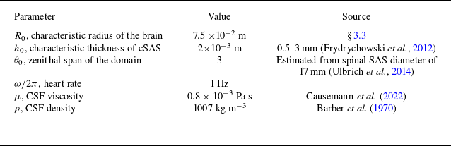

 Ng=10
 z

 θ=0
 η
 t1=0.88T
 t2=0.11T
 t3=0.5T
 T
 T=2π
 θ
 θ
 u¯θ0
 θ=θ0
 η
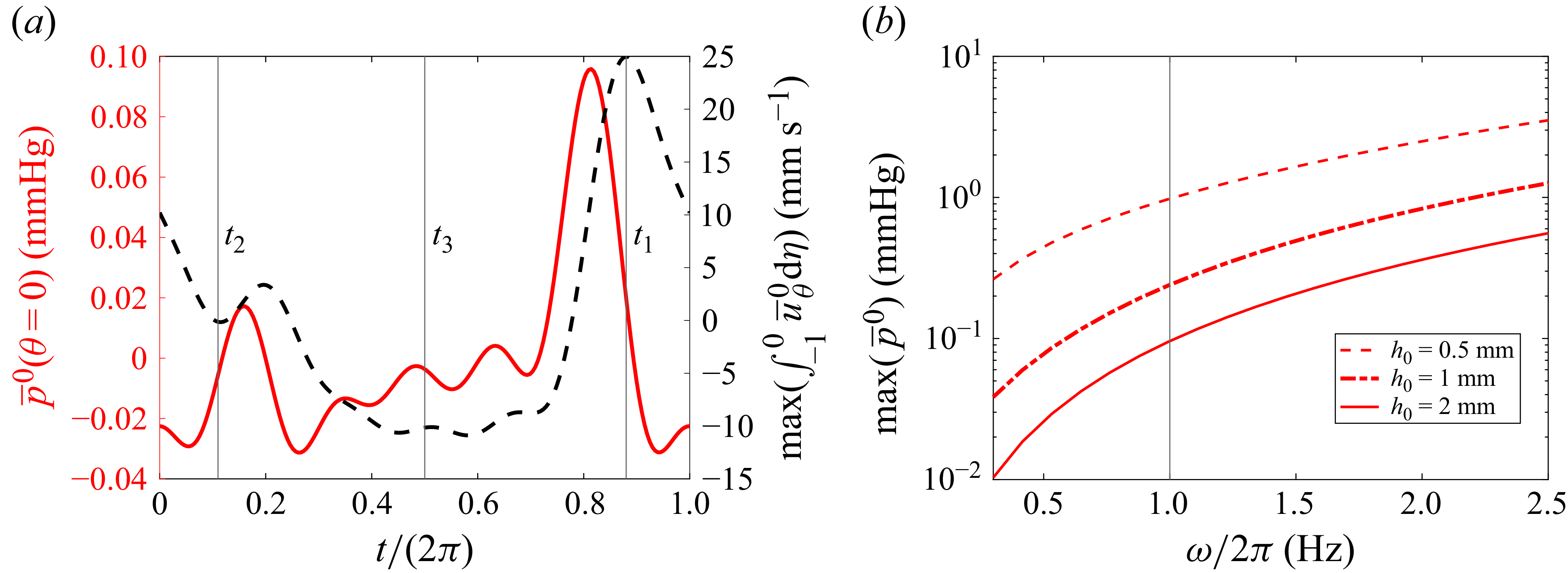
 θ=0

 t1=0.775T
 t2=0.14T
 t3=0.5T
 v¯ξ
 y=0
 x=0
 η

 θ=0
 θ=π/2
 ∫02πp¯0dϕ/2π
 ω
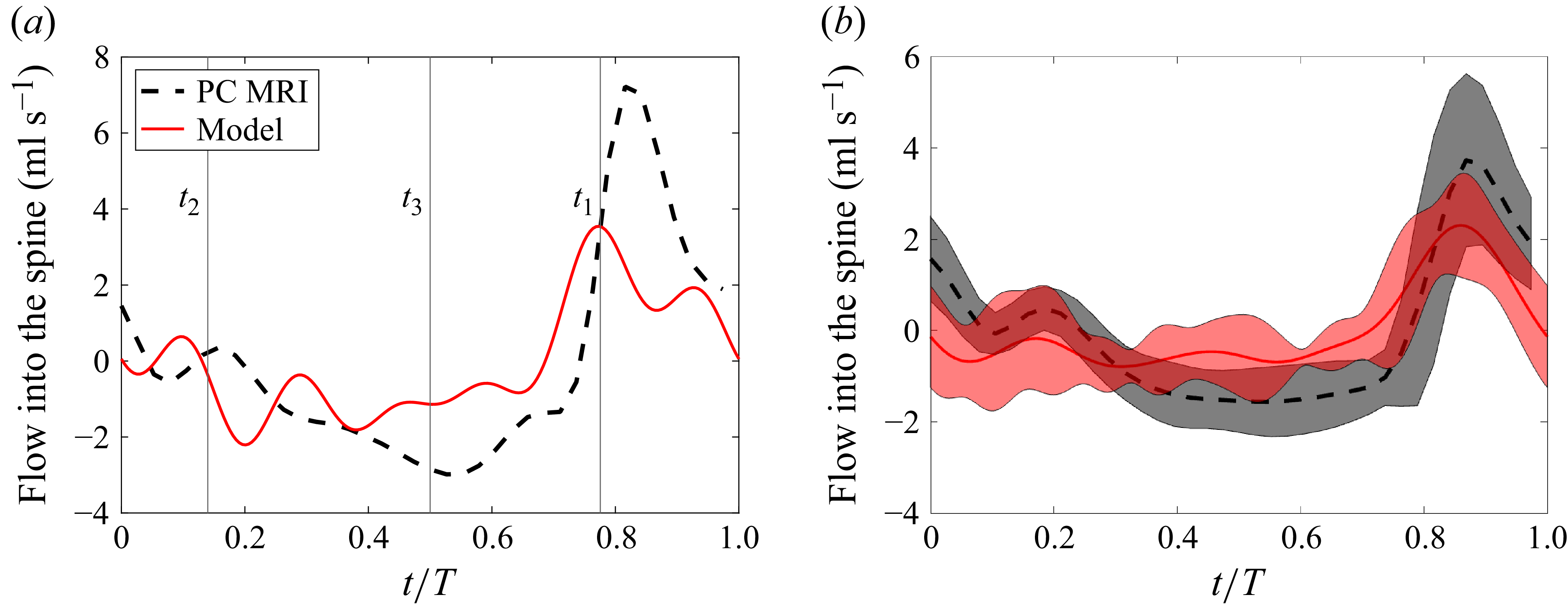
 ∫δSu0⋅e2/e22dS=∫−10∫02πe33(uθ0+uϕ0e23/e22e33)dϕdη
 t1
 t2
 t3
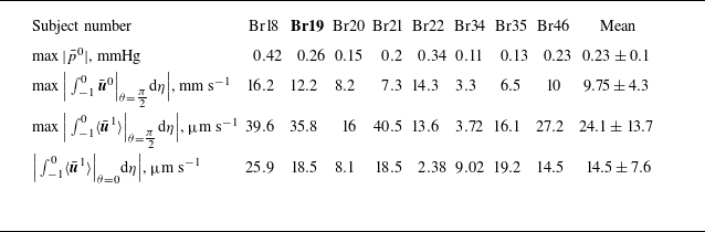
 θ=π/2
 θ=π/2
 θ=0

 η
 uξ1
 p¯1
 θ
 u¯θ1
 θ=θ0

 d(t)

 p¯1
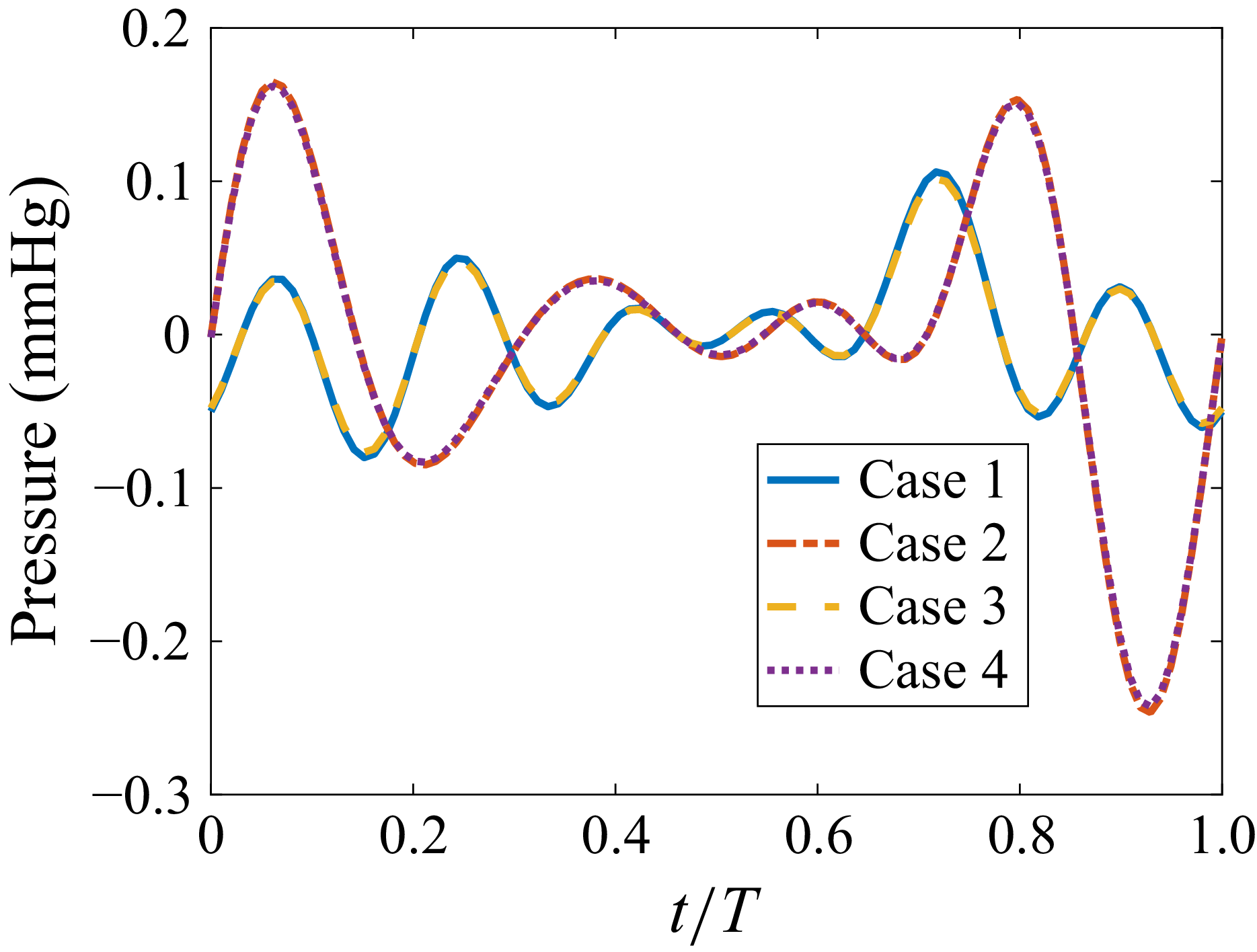
 θ=0


 Open access


