1 Introduction
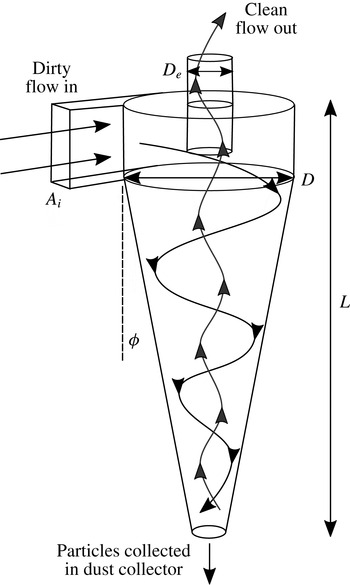
A cyclone separator is a device used to separate particles from a fluid using centrifugal forces in a rapidly swirling flow. Separators can vary in size from large industrial machines to small devices incorporated into household vacuum cleaners. Cyclone separators are typically cylindrical or conical and the swirling flow is generated by a tangential inlet. Figure 1 shows a typical configuration for a cyclone separator. Dirty air enters through the inlet with area
 $A_{i}$
, particles are separated into a collecting receptacle at the bottom of the cone, and clean fluid leaves via the outlet at the top through a vortex finder (diameter
 $D_{e}$
).
The swirling flow inside a cyclone separator produces hydrodynamic oscillations that manifest as noise for the small cyclones used in vacuum cleaners. In the case of large industrial scale cyclones, such oscillations can also lead to structural damage. Chanaud (Reference Chanaud1965) carried out visualisation experiments on cyclones and vortex whistles using dye to reveal the unsteady motions. This revealed that the core of the vortex deviates from the centre of the device and undergoes precession. This motion is referred to as a precessing vortex core (PVC). It was concluded that in both devices the precession is derived from a hydrodynamic instability of the flow. However, no quantitative details about the mechanism could be determined. The experiments indicated the relevant dynamical parameters as the Strouhal, Rossby and Reynolds numbers.
Typical cyclone separator design and geometry.

The same phenomenon of vortex core deviation and precession was observed in a cyclone separator by Peng et al. (Reference Peng, Hoffmann, Dries, Regelink and Stein2005) using dust particles within the flow. The frequency of the precession, measured using a stroboscope, was linearly proportional to the volumetric flow rate. In this case, it was found that the vortex core could deviate sufficiently to become attached to the outer walls in their cylindrical separator. A conical separation chamber is known to have a stabilising effect on vortex core motions because of the constraining effect of the narrowing walls. However, even in these cases, precession can occur.
Quantitative measurements of the internal flow oscillations have been made using hot-wire anemometry. Yazdabadi, Griffiths & Syred (Reference Yazdabadi, Griffiths and Syred1994a ) used this method to detect the velocity fluctuation from the regular passage of the PVC and to analyse the occurrence of the fluctuations as a function of the Reynolds number and swirl number. As the Reynolds number increased, the Strouhal number of the oscillation was found to asymptote towards a constant value.
The principle of this technique was extended by using laser Doppler anemometry (LDA). Yazdabadi, Griffiths & Syred (Reference Yazdabadi, Griffiths and Syred1994b ) used a cyclically triggered measurement tied to the PVC frequency to generate a picture of the instantaneous flow and the displaced core at one point in the cycle. Using this technique, their study investigated how variations in outlet geometry inhibit the presence of a PVC.
Grimble & Agarwal (Reference Grimble and Agarwal2015) showed by means of hot-wire anemometry inside the cyclone and microphone measurements outside the cyclone that the hydrodynamic oscillations of the vortex core are highly correlated with a nearly tonal acoustic noise, which was called a ‘cyclone hum’. Thus, they could use acoustics as a proxy to characterise the oscillations. As external acoustic measurements are much easier to obtain compared with internal flow measurements, the authors were able to make measurements for several parametric settings. The non-dimensional parameters that determine the dynamics of the vortex core were identified as a modified Strouhal number, the Reynolds number, a geometry based swirl number and numerous geometric scales defining the shape of the device. The results produced an excellent collapse of the data, yielding a simple relationship for the Strouhal number as a function of the swirl number and the outlet diameter ratio. A heuristic model was presented for the hydrodynamic oscillations. The aim of this paper is to study the flow inside the cyclone through flow visualisation and further examine the hydrodynamic oscillation and the causal mechanisms by means of linear stability analyses.
The simplest model for the flow inside a cyclone is a Rankine vortex with an axial plug flow. The stability of this model flow was studied by Loiseleux, Chomaz & Huerre (Reference Loiseleux, Chomaz and Huerre1998). Their study looked at changes in stability characteristics as a result of changes in the swirl magnitude and nature of the axial flow (wake, jet, co-flow or counter-flow) for a range of azimuthal wavenumbers.
Nevertheless, the real cyclone geometry does not extend infinitely as an ideal parallel flow. The application of stability analysis to spatially varying flows was reviewed by Huerre & Monkewitz (Reference Huerre and Monkewitz1990), where they highlighted that when the base flow changes very slowly along its length, it is possible to consider the local stability of each streamwise position in the flow independently. An example of this concept was carried out by Qadri, Mistry & Juniper (Reference Qadri, Mistry and Juniper2013) to study the unsteady modes of vortex breakdown. The local stability analysis was able to isolate the regions of absolute instability that lie around the recirculation bubble and identified that a spiral mode with azimuthal wavenumber
 $m=-1$
develops on top of this base flow.
In this paper, we will carry out such a stability analysis on the simulated flow of a cyclone separator and compare the results with experimental observations of the oscillations. The methodologies for the visualisation experiments and local stability analysis are presented in §§ 2 and 3 respectively. In § 4, we will present the results of the two experimental techniques and analyse the key locations in the flow that exhibit unsteady behaviour. The results of the stability analysis will be presented in § 5 and compared with the experimental observations. Finally, in § 6, we will present the conclusions from the analysis and suggest where this research will lead for future work.
2 Visualisation experiments
Two techniques have been used to measure the flow field inside the cyclone. The first uses a water visualisation rig, because particle visualisation is easier to achieve in water. The second technique measures the internal fluctuations in air using a hot-wire anemometer.
Throughout all experiments, the cyclone design was identical to the one used for acoustic testing described in Grimble & Agarwal (Reference Grimble and Agarwal2015) (cyclone length
 $L=15$
cm), against which we will be comparing the results of the experiments of this paper.
The present experiments achieve dynamic similarity between air and water in order to explore a small number of specific geometries in detail using a range of techniques. Dimensional analysis of the cyclone system (see Grimble & Agarwal (Reference Grimble and Agarwal2015) for more details) shows that the predominant acoustic frequencies
 $f$
measured in the system, governed by hydrodynamic processes, can be described by a Strouhal number,
 $St=f{D_{e}}^{3}/QSw$
. The Strouhal number is scaled by the volumetric flow rate
 $Q$
and the vortex finder diameter
 $D_{e}$
, which is found to be the key length scale. The swirl number
 $Sw=DD_{e}/A_{i}$
is an important geometric ratio describing the swirl intensity for a system (Gupta, Lilley & Syred Reference Gupta, Lilley and Syred1984; Yazdabadi et al.
Reference Yazdabadi, Griffiths and Syred1994b
). In the Strouhal domain, flow-dependent frequencies of the system are highlighted, as they collapse to a single value, while geometric resonances are spread out. This allows the two phenomena to be distinguished through variations of the flow rate. The Strouhal number is found to be dependent on the Reynolds number,
 $Re=\unicode[STIX]{x1D70C}Q/\unicode[STIX]{x1D707}D$
(based on
 $Q$
and the fluid density
 $\unicode[STIX]{x1D70C}$
and viscosity
 $\unicode[STIX]{x1D707}$
), and a host of geometric parameters based on the dimensions shown in figure 1, most notably the swirl number,
 $Sw$
and the outlet area ratio,
 $D_{e}/D$
,
 $$\begin{eqnarray}\displaystyle & \displaystyle \frac{f{D_{e}}^{3}}{QSw}=F\left(\frac{\unicode[STIX]{x1D70C}Q}{\unicode[STIX]{x1D707}D},\frac{D}{D_{e}},\frac{DD_{e}}{A_{i}},\frac{L}{D_{e}},\unicode[STIX]{x1D719},\frac{Q}{c{D_{e}}^{2}}\right), & \displaystyle\end{eqnarray}$$
 $$\begin{eqnarray}\displaystyle & \displaystyle St=F\left(Re,\frac{D}{D_{e}},Sw,\frac{L}{D_{e}},\unicode[STIX]{x1D719},M\right). & \displaystyle\end{eqnarray}$$
This dependence suggests that dynamic similarity between air and water can be achieved by matching the Reynolds number and other geometric ratios between the two systems. We cannot match the Mach number (
 $M$
). Because
 $M$
is small, the influence of compressibility is negligible and variations in
 $M$
can be ignored. The difference in density and viscosity between air and water implies a reduction in the flow rate for the water system by a factor of approximately 13 to match the
 $Re$
in air. This shift in flow rate also means that the observed frequencies of the system shift by the same factor. This results in frequencies of the order of hundreds of Hertz rather than thousands, which allows greater time resolution for visualisation.
2.1 Water visualisation design
The primary visualisation component of the experiment rig was a transparent cyclone separator bored from a solid Perspex block. This core cyclone was designed to be used with modular parts for the vortex finder in order to investigate the influence of varying the outlet area ratio and swirl number. A Perspex tube was fitted at the base of the cone to act as a sealed dust collector. A tube was also fitted downstream of the vortex finder to allow visualisation of the flow as it leaves the cyclone.
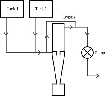
An outline of the rig components and flow path is shown in figure 2. Controllable water flow was achieved using a combination of header tanks attached to the mains water supply and control valves. The header tanks and valves alone could generate a range of flow rates. Higher flow rates could be achieved using an electric central heating pump that was attached downstream of the cyclone to apply suction. The cyclone was linked to the water supply with a parallel bypass channel. This enabled a greater range of flow rate control, in particular enabling low flow rates. The bypass path was also critical to prevent stalling of the pump when closing supply valves. The flow was exhausted to atmospheric pressure downstream of the pump at a fixed height relative to the header tanks.
Flow schematic and layout of the visualisation experiment. The two supply tanks provide either a clean or a seeded water supply. The pump and bypass line allow full control of flow rates.

The various components of the rig were connected via
 $1/2$
inch pipes. The pipe arrangement and component position and orientation were dictated by the need to ensure that air would not be trapped within the system. Flow rate measurement was achieved by using a combination of an orifice plate flowmeter and measuring the time for a known mass of water to be ejected at the downstream end of the rig. Five repeated measurements were carried out for set operating conditions and pump speeds and the flow rate was found to be consistent over the multiple measurements (table 1). These operating conditions overlap with the equivalent operating points for measurements carried out in air (see Grimble & Agarwal Reference Grimble and Agarwal2015). Given the observation that the Strouhal number was only weakly dependent on the Reynolds number, a small number of easy to repeat flow rate conditions were chosen for tests, since the primary focus of the study was on how the flow structures were affected by the outlet geometry.
Flow rate measurements for the water rig. The flow conditions were found to be highly repeatable for the same valve and pump configurations. Representative Reynolds numbers are indicated for each flow rate for a cyclone geometry with reference inlet and outlet area
 $A_{0}$
. Acoustic experiments in air were carried out for Reynolds numbers ranging from
 $1.9\times 10^{3}$
to
 $6.6\times 10^{3}$
.

The water supply was split into two header tanks. One of these was kept as a clean water supply and the second had seeding particles added. Quick-turn valves allowed the two supplies to be rapidly switched and allowed pulsing of seeding materials into the cyclone. The heights and flow paths of the two tanks were identical in order to ensure the same delivery pressure. The chosen particles were fine polyvinyl chloride granules. These particles were slightly denser than water and therefore slowly sank when the water flow was off. By agitating the settled dust in the header tank, it became suspended and allowed control of the particle concentration of the flow. The solids loading of the cyclone is known to affect the flow dynamics, but this parameter was beyond the scope of this investigation and was kept low to limit any effect on the flow (
 $\mathit{mass}_{\mathit{particles}}/\mathit{mass}_{\mathit{water}}<0.001$
).
The main visualisation tool for the flow was a high-speed video camera capable of frame rates up to 10 kHz. The target oscillation was expected to be of the order of 100 Hz due to the flow rate reduction from using water. Therefore, a frame rate of up to 2 kHz was used to provide sufficient frames to resolve the oscillations. Large frame rates come with the penalty of reduced sensitivity of the camera due to faster shutter speeds. Depending on the particular test being carried out, a frame rate was chosen based on an optimisation of sufficient time resolution and light levels.
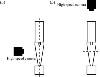
A Photron FASTCAM ultima APX 120K was used with a large-aperture lens, which provided a very narrow depth of field in order to isolate just the illuminated plane. This also maximised the amount of light into the camera at the high frame rates. The narrow focal plane could be used for looking at planes deep inside the cyclone by focusing through the Perspex rig. An example of the camera positioning and lighting set-up is shown in figure 3(a,b), where the camera is focused on a vertical and horizontal plane respectively inside the cyclone.
Camera position and lighting set-up for vertical (a) and horizontal (b) slice illumination. The collimated light sheet plane is indicated by the dashed line relative to the high-speed camera location.

Additional lighting was key for ensuring that there was enough brightness for the given frame rate and camera sensitivity. For particle seeding, a narrow plane of the flow was illuminated using a collimated light source. By keeping the environment dark, this served to capture the particle motions in just that plane. The collimated light source could be angled to illuminate a plane at any angle inside the cyclone.
2.2 Hot-wire anemometry
An identical Perspex-based cyclone was used as the basis for hot-wire anemometry tests. Perspex allows the wire to be seen while being inserted, thus preventing breakages and damage from coming into contact with the walls. The surfaces of the block provided a rigid mounting point for a radial traverse system.
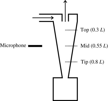
The hot-wire rig layout showing the cyclone layout and microphone location outside the cone. The radial traverse positions are shown as dotted lines.

The hot-wire system was mounted on a traverse that could be inserted through the cyclone wall (figure 4). The hot-wire probe was a single straight wire (Dantec model 55P11). The use of a single straight hot-wire probe in the experiment meant that the measurement was only sensitive to velocity magnitude and not direction. The probe was inserted radially, but could be rotated such that it was sensitive to either the axial or the azimuthal velocity. The wire orientations also meant that it was always sensitive to radial velocities. However, the radial flow component was assumed to be small relative to the axial and azimuthal components and could be neglected (see figure 5).
A bell-mouth inlet identical to the one used in the acoustic measurements carried out in Grimble & Agarwal (Reference Grimble and Agarwal2015) was mounted on the inlet with a smooth round to square transition pipe connecting it to the tangential slot inlet of the cyclone. The outlet flow was ducted away from the outlet and the flow was driven by a compressor far downstream to isolate the noise from the apparatus.
3 Hydrodynamic stability analysis
3.1 Simulations of cyclone flow
In order to carry out a stability analysis, mean flow data are required upon which the small linear oscillations are modelled. Hoekstra, Derksen & Van Den Akker (Reference Hoekstra, Derksen and Van Den Akker1999) carried out LDA measurements of the mean flow inside a cyclone and used these experiments to validate a number of Reynolds averaged Navier–Stokes (RANS) models. The best agreement was observed with the Reynolds stress turbulence model (RSM), whereas the
 $k{-}\unicode[STIX]{x1D716}$
models were unable to model the swirling component of the vortex flow correctly. The RSM evaluates each term of the turbulent stresses and allows the effects of swirl on the turbulent transport to be modelled (ANSYS 2011). It has been observed in many studies that the RSM is able to accurately capture the internal flow dynamics (Hoekstra et al.
Reference Hoekstra, Derksen and Van Den Akker1999; Gimbun et al.
Reference Gimbun, Chuah, Choong and Fakhru’l-Razi2005). Slack et al. (Reference Slack, Prasad, Bakker and Boysan2000) observed that the RSM accurately captured the swirl and axial velocity profiles, when compared with LDA measurements. The mean flow data used for this analysis were taken from steady axisymmetric RANS simulations using the RSM. The simulations were carried out using ANSYS Fluent.
Pisarev et al. (Reference Pisarev, Gjerde, Balakin, Hoffmann, Dijkstra and Peng2012) were able to compare the displacement of the vortex core observed in the experiments of Peng et al. (Reference Peng, Hoffmann, Dries, Regelink and Stein2005) with simulations. The precession behaviour could also be observed with 3D unsteady simulations using both RANS and large-eddy simulation to model the turbulent flow (Derksen & Van den Akker Reference Derksen and Van den Akker2000; Gronald & Derksen Reference Gronald and Derksen2011). It was observed that the vortex was initially centralised at low flow rates before becoming displaced, and that a stability analysis of that initially steady flow could reveal the factors influencing vortex displacement.
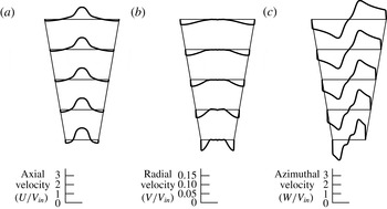
A typical RANS simulation is shown in figure 6. The tangential inlet is modelled as a fixed mass flow with a set direction vector. Due to the axisymmetric nature of the simulation, the single inlet is modelled as a distributed mass flux around the entire circumference of the cyclone, with the magnitude of the inlet swirl velocity relative to the radial velocity determined by the effective inlet size.
Internal measurements of cyclone velocity components from 2D RANS simulations at various axial locations: (a) axial, (b) radial and (c) azimuthal components. All velocities are normalised by a reference velocity,
 $V_{in}$
, based on the cyclone inlet conditions.

The simulations use a structured quadrilateral grid that converges towards the cone tip by keeping the number of radial mesh vertices the same along the length of the cyclone. This is necessary to ensure that the swirl flow propagates all the way to the cone tip and provides high mesh resolution in this region to resolve the strong flow gradients that are present. The focus of the validation was to compare the strength of the swirl and centrifugal acceleration at the cone tip with the expected separation performance from experiment. The separation performance can be used to infer the strength of the swirl empirically (Cortes & Gil Reference Cortes and Gil2007). The mesh resolution was determined by the number of radial cells required to accurately capture a combined vortex profile at the narrowest point in the cyclone. This design of cyclone has been extensively studied as part of the product design process. It is therefore well characterised by experiments, and its performance and flow structure are well understood.
The outlet tube is long so that a fixed pressure outlet boundary condition can be applied far downstream. This prevents it from interfering with the flow in the conical chamber.
3.2 Local stability analysis
The Reynolds number (based on cyclone diameter) of a typical flow rate used in our study is of the order of
 $10^{4}$
. The flow field is turbulent. The unsteady flow within a cyclone can be thought of as a combination of coherent large-scale eddy motions and random turbulent motions around the time-averaged mean flow (Reynolds & Hussain Reference Reynolds and Hussain1972). The applicability of a linear stability analysis around a time-averaged mean flow has been discussed by a number of authors including Mettot, Sipp & Bézard (Reference Mettot, Sipp and Bézard2014), Turton, Tuckerman & Barkley (Reference Turton, Tuckerman and Barkley2015) and Tammisola & Juniper (Reference Tammisola and Juniper2016).
Previous work by Meliga, Pujals & Serre (Reference Meliga, Pujals and Serre2012) used the eddy viscosity for simulations of the stability of a wake flow. The findings of Mettot et al. (Reference Mettot, Sipp and Bézard2014) showed that turbulence has only a weak effect on the linear stability analysis, and the behaviour can be accurately captured using the molecular viscosity. Oberleithner et al. (Reference Oberleithner, Sieber, Nayeri, Paschereit, Petz, Hege, Noack and Wygnanski2011) and Juniper (Reference Juniper2012) also showed that molecular viscosity was sufficient to model the behaviour of swirling flows when using a local stability analysis, and this assumption is applied here for the analysis of the cyclone.
To carry out the local analysis, the flow is split into slices perpendicular to the central axis. The WKBJ approximation is used, which assumes that the wavelength of perturbations is significantly shorter than the length scale over which the base flow changes. This approximation assumes that the flow is parallel and ignores any radial velocity from the base flow, but is also found to work well for flows that are significantly non-parallel (Pier Reference Pier2008). In the case of the cyclone, the flow is close to parallel inside the main conical separation chamber, as can be seen in figures 5 and 6. However, there are significant radial velocities as the flow expands beyond the cone tip into the dust collector, and as it enters the outlet duct (vortex finder), where these assumptions may break down (figure 6).
Local analysis domain sections overlaid on contours of swirl velocity (linear colour scale increasing from blue to red). The axial and radial velocity components are shown as arrows. The flow can be seen to be close to parallel within the main cone of the cyclone and into the outlet as radial components are small.

By performing a Fourier/Laplace decomposition of the flow perturbations, the unsteady flow is modelled as harmonic in time and in the streamwise direction with an angular frequency
 $\unicode[STIX]{x1D714}$
and an axial wavenumber
 $k$
. Azimuthal variations are modelled by given values of an azimuthal wavenumber,
 $m$
. The perturbations are assumed to be of the form
 $f(r)\text{e}^{\text{i}(kx+m\unicode[STIX]{x1D703}-\unicode[STIX]{x1D714}t)}$
. This results in the governing equations reducing to an eigenvalue problem that is satisfied for eigenvalue pairs of
 $k$
and
 $\unicode[STIX]{x1D714}$
(Huerre & Monkewitz Reference Huerre and Monkewitz1990; Huerre Reference Huerre, Batchelor, Moffatt and Worster2000). A no-slip boundary condition is imposed at the outer wall. At the centreline, symmetry conditions are imposed, which depend on the value of
 $m$
.
The local stability analysis is performed with the software package InstaFlow, described in Juniper, Tammisola & Lundell (Reference Juniper, Tammisola and Lundell2011) and Tammisola (Reference Tammisola2011). For each streamwise slice of the flow, the velocities are projected onto Gauss–Lobatto-spaced points in the radial direction. The governing equations and boundary conditions are expressed in matrix form using Chebyshev differentiation matrices. At each slice, this generates a matrix eigenvalue problem for
 $\unicode[STIX]{x1D714}$
in terms of
 $k$
. Saddle points of
 $\unicode[STIX]{x1D714}(k)$
are found and their Briggs–Bers validity is checked (Bers Reference Bers, Galeev and Sudan1983). These saddle points are then tracked as the streamwise location changes. The focus of the analysis in this paper will be on comparing the spatio-temporal stability characteristics with the experimental observations of the unsteady flow in the cyclone.
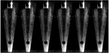
Time lapse of an illuminated plane of particles through the centre inside the cyclone cone. The separation mechanics reveals the position of the core and shows unsteady behaviour, most notably at the cone tip. The dark spot near the cone tip is one of the dye injection points on the outer surface of the rig. The images are sequential frames taken at a rate of 1000 fps.

3.3 Parameter variations
The RANS simulations were generated for a number of different flow conditions based on the parameters derived through dimensional analysis (2.1) and (2.2) previously used in the experiments to measure the acoustic behaviour (Grimble & Agarwal Reference Grimble and Agarwal2015). Reynolds number variations were achieved by varying the mass flow rate at the inlet. The swirl number of the flow was varied with both inlet and outlet area changes. Different inlets were modelled by changing the azimuthal velocity relative to the radial component. The swirl velocity,
 $V_{\unicode[STIX]{x1D703}}$
, at the inlet is based on a uniform inlet velocity across the inlet with area
 $A_{i}$
,
 $V_{\unicode[STIX]{x1D703}}=Q/A_{i}=Q/ab$
(
 $a$
and
 $b$
are the height and width respectively of the rectangular tangential inlet section). However, the radial inflow,
 $V_{r}$
, in the axisymmetric model is distributed around the whole circumference, such that
 $V_{r}=Q/\unicode[STIX]{x03C0}Da$
. Therefore, the ratio of swirl and radial velocities necessary at the inlet is
 $V_{\unicode[STIX]{x1D703}}/V_{r}=\unicode[STIX]{x03C0}D/b$
. Swirl number variations were also achieved by changing the vortex finder diameter
 $D_{e}$
, which required a change in the mesh and geometry.
4 Experimental results and discussion
4.1 Particle visualisation
Figure 7 shows a typical slice through the centre plane of the separator viewed from the side. The image is a series of snapshots taken from high-speed video capture. The separation mechanics of the flow produces a clean core, allowing its position to be viewed. The position of this separation surface (the transition from clean to dirty flow) is unsteady and shows that the underlying flow is also unsteady.
The strongest unsteadiness is observed at the cone tip. The clean central core is seen to deviate significantly from the centreline. The vortex core is also less distinct at the cone tip, which is a sign that the unsteady flow disrupts the separation of particles and leads to some being recaptured by the flow.
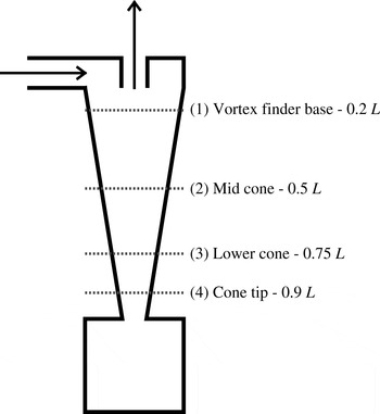
In order to more accurately measure the rotation rates and frequencies of the disturbances, the high-speed camera was positioned above the cyclone and focused onto an illuminated slice through the vortex finder. Figure 8 shows the positions of the slices examined for the different cyclone configurations.
Positions of horizontal imaging locations relative to the cyclone. Heights are given as a fraction of the cyclone length,
 $L$
.

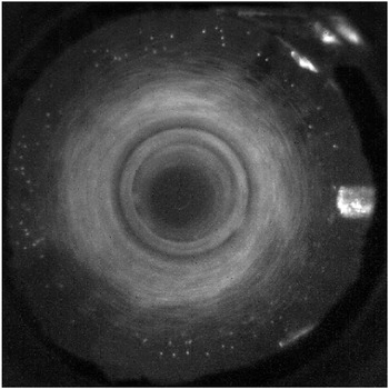
Illuminated particles in a horizontal slice through the top of the cyclone just below the vortex finder (slice 1). The dark area at the centre shows that the particles have been successfully separated and are not entering the vortex finder. The cone roof is manufactured out of Perspex to allow the whole cyclone diameter to be visible.

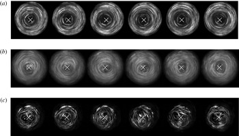
Figure 9 shows the illuminated particles just below the vortex finder at position 1. The central vortex core is very clean and there are few particles near the centre with which to visualise the flow. The situation is significantly different further down the cone. Figure 10 shows a time lapse of the illuminated particles at horizontal slices 2, 3 and 4. The geometric centre is marked by a white cross. It is clear that the swirling flow is precessing about the centre. At slice 2, the core position can be seen to deviate slightly from the geometric centre of the system (figure 10 a). This trend continues moving further down the cyclone, with larger and more visible deviations at slice 3 (figure 10 b).
Subsequent frames showing small deviations of the vortex centre with time; (a), (b) and (c) respectively correspond to slices 2, 3 and 4 in figure 8. The frame rate is 250 fps using an outlet area of
 $2A_{0}$
for all cases.

The flow at slice 4 (figure 10 c) reveals a more complicated flow structure. Two separate centres of rotation can be seen spinning symmetrically about the centre of the cyclone. The top-down view shows more clearly that it is a symmetric bifurcation of the vortex core and the sense of rotation of each vortex is the same as that of the parent vortex.
4.2 Frequency measurements from high-speed video
The rotation frequency of the unsteady phenomena can be estimated by counting the number of image frames for a certain number of cycles. However, in many cases there is clearly more than one distinct frequency component to the oscillations. In order to generate a more accurate picture of the frequency content of the oscillations at different points, the temporal variations of small sections of each high-speed video were examined and spectrally analysed.
For each video, a small section of the image was isolated based on the desired measurement location. This was typically a 10–20 pixel square corresponding to a real scale region of the order of 1 mm in size. The light exposure of this region was then quantified for each video frame to effectively measure the passage of particles through that region. This was done by summing the magnitude of all of the pixels in the region.
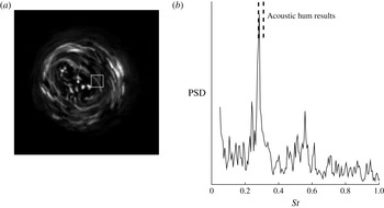
Figure 11 shows the spectral measurement for the video sequence shown in figure 10(c) from the cone tip. Two strong peaks can be seen corresponding to the passage of two vortex cores rotating around a common centre.
The power spectral density (PSD) taken from the image (a) of the top-down view of the cyclone vortex tip from within the marked square. There are two clear peaks in the spectrum (b) corresponding to the dual-core phenomenon that has been observed at
 $St=0.28$
and
 $St=0.56$
. The Strouhal number range measured using acoustics (Grimble & Agarwal Reference Grimble and Agarwal2015) is indicated and shows a match between the non-dimensional results of the two experiments.

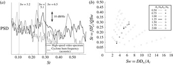
Further spectral measurements of cyclones with different vortex finder diameters are shown in figure 12. Measurements have been taken from the cone tip (slice 4 in figure 8) because the oscillations are strongest at this location. Comparison of the peaks in these spectra with the acoustic modes measured on the same geometries in air (Grimble & Agarwal Reference Grimble and Agarwal2015) shows that the Strouhal number varies with the swirl number in the same way. This indicates that the phenomena observed in water experiments are the same as those that cause the acoustic hum observed in air experiments.
Comparison of high-speed video spectra and acoustic measurements from Grimble & Agarwal (Reference Grimble and Agarwal2015) with three different outlet diameters,
 $D_{e}/D=0.17$
, 0.26 and 0.33. These correspond to swirl numbers of 3.2, 5.1 and 6.5 respectively. The raw spectral data from the high-speed imagery are shown in (a). The frequencies of the spectral peaks are shown as filled markers in (b) in context with the full range of
 $Sw$
and
 $D_{e}/D$
parameters that were tested by Grimble & Agarwal (Reference Grimble and Agarwal2015) (open markers).

4.3 Flow dynamics from anemometry
Hot-wire anemometer measurements (in air) were used to detect the locations of peak oscillations with radial traverses at each of the three axial stations shown in figure 4. The aim is to compare the measured fluctuations with the hydrodynamic oscillations observed in water in order to demonstrate dynamic similarity between air and water. The cyclone used in this test had a swirl number of
 $Sw=5.1$
and a vortex finder diameter of
 $D_{e}/D=0.26$
.
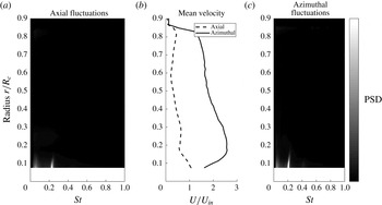
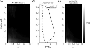
Figure 13 shows the spectra of velocity fluctuations as a function of radius (scaled by the maximum cyclone cone radius
 $R_{c}$
) for both the azimuthal and axial measurements. Close to the central axis, there is a strong narrow-band fluctuation. This is isolated to the vortex core and disappears beyond
 $0.15R_{c}$
from the central axis. The Strouhal number of approximately 0.22 matches the acoustic noise measurements and high-speed video observations of this geometry. A high-pass filter was employed to eliminate the DC offset of the measurement, which would otherwise dominate and mask the unsteady motions being examined here. The cutoff frequency is at a Strouhal number of approximately 0.03.
Hot-wire anemometer spectrum sweep with changing radius at the top axial station (see figure 4). Axial fluctuations are shown in (a) and azimuthal fluctuations in (c). These are aligned radially with the mean flow profiles in (b) to highlight the regions of the flow where oscillations are observed. Radii are non-dimensionalised by the maximum radius of the cyclone cone
 $R_{c}$
(at the top of the cone). Due to the limits of the hot-wire traverse, it was not possible to reach the centreline with the available travel of the probe; hence, there are no data for
 $r/R_{c}<0.1$
.

Figure 14 shows the same frequency analysis for the middle station. There is no single distinct frequency of oscillation in either the axial or azimuthal measurements. This shows that there is no measurable coherent precession in this region.

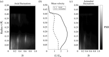
Figure 15 shows the spectral signature for the third station close to the cone tip. In this case, there are strong coherent fluctuations at
 $St\approx 0.3$
. In addition, there is a second mode that is approximately a harmonic at
 $St\approx 0.6$
, which can be most clearly seen in the axial spectrum. The first mode is close in frequency to the single dominant spectral peak detected at the top of the cone and will be referred to as mode 1. The intensity of low-frequency noise (
 $St<0.1$
) is greater at this position compared with the top of the cone (figure 13).
The mode 1 peak has a Strouhal number approximately 30 % larger at the cone tip than the value measured at the top station. This shift may be a result of the restriction caused by the hot-wire probe in the flow. The maximum achievable flow rate for the system was reduced when the probe was at the cone tip. This indicates greater losses in the system with this configuration. The cone tip is likely to be more susceptible to the blockage effects of the hot wire due to the reduction in diameter. The second frequency (mode 2) is approximately double the first but is not necessarily a harmonic. The oscillating area of the flow is a finite region within a radius of
 $0.15R_{c}$
from the geometric centre. This position is close to the location of peak azimuthal velocity in the mean flow profile.
It is noted that the azimuthal velocity measurement does not reach zero at the centreline of the system. This may be a result of vortex precession in the system continuously shifting the position of the centre of rotation. As the hot wire is only sensitive to magnitude and not direction, this would register as a non-zero magnitude on average. Similar observations were made in LES simulations of cyclones by Derksen & Van den Akker (Reference Derksen and Van den Akker2000), where vortex precession was observed, leading to non-zero time-averaged swirl velocities at the cyclone centre.

Comparing the results of oscillation measurements in both air and water, it can be seen that similar frequency behaviour is observed at the top and tip of the cone. The cases represented in figures 12 and 15 use identical cyclone geometries.
4.4 Acoustic correlation
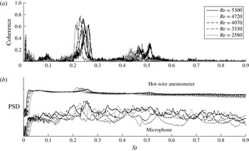
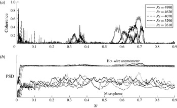
The hot-wire frequency peaks are found to vary with the flow rate and tend towards a constant Strouhal number at higher flow rates. In order to determine the coupling between the internal flow oscillations and external sound, a microphone was positioned outside the rig in conjunction with the hot wire to simultaneously measure the two phenomena. Figures 16 and 17 display the spectra of the two measurements at the top and tip of the cyclone at the radius where oscillations could be detected for the axial hot-wire orientations (
 $0.1R_{c}$
). The coherence between the microphone and anemometer measurements (
 $C_{xy}(f)$
) is also shown and is defined based on the cross-spectral (
 $G_{xy}(f)$
) and auto-spectral densities (
 $G_{xx}(f),G_{yy}(f)$
) of the two signals
 $x$
and
 $y$
respectively as
 $$\begin{eqnarray}C_{xy}(f)=\frac{|G_{xy}(f)|^{2}}{G_{xx}(f)G_{yy}(f)}.\end{eqnarray}$$
Hot-wire anemometer (aligned with axial velocity) and external microphone coherence (4.1), and power spectral density measurements at the top axial station. The frequency is non-dimensionalised as a Strouhal number. The first mode has a Strouhal number between 0.21 and 0.26 (the variation is due to a weak Reynolds number dependence on the frequency behaviour) and shows strong coherence between the hydrodynamic fluctuations and external sound spectra. A second mode at approximately
 $St=0.5$
shows much weaker coherence.

As figure 16 but with the hot wire measuring at the tip axial station. Strong coherence is now observed with mode 2.

From figures 16 and 17, the constant-Strouhal-number modes can be clearly observed, although there are small shifts in the Strouhal value for different flow rates, indicating a weak Reynolds number dependence. These observations are consistent with the acoustic hum frequency reported in Grimble & Agarwal (Reference Grimble and Agarwal2015). The equivalent geometry was found to exhibit a Strouhal number range between 0.23 and 0.26, which matches the values measured in this experiment. The cyclone hum noise correlates strongly with the mode 1 frequency fluctuations at the top of the cyclone cone. At this position, only a weak mode 2 signal is detected by the hot wire, showing that mode 1 is dominant. However, at the tip of the cyclone, the correlation is strongest with mode 2 fluctuations. This is partly because mode 2 is dominant in the hot-wire spectrum at this position in the cyclone, but also because the mode 1 velocity fluctuations no longer match the frequency of the hum. Comparing figures 16 and 17, there is a small increase in the externally measured hum Strouhal number as a result of moving the internal anemometer probe from the top to the tip of the cyclone. This can be explained by the increased blockage and disruption of the swirl flow. However, the mode 1 hydrodynamic fluctuation increases in frequency by a larger amount and no longer produces strong coherence between the two signals.
It can be seen from the differences in coherence between figures 16 and 17 that there are clear changes in the flow dynamics along the length of the cyclone vortex. There is an increase in oscillation frequency by moving from the top of the cone towards the narrow tip. The radial location of the oscillations remains consistent at approximately
 $0.15R_{c}$
from the central axis, which is close to the peak of the azimuthal velocity. On examining the mean flow profiles in figures 13 and 15, it can be seen that the peak azimuthal velocity increases towards the bottom of the cyclone. The oscillation frequencies therefore appear to be determined by the angular velocities, as postulated by the heuristic model in Grimble & Agarwal (Reference Grimble and Agarwal2015).
5 Local stability analysis results
5.1 Axisymmetric modes
The first case examined using local stability analysis was axisymmetric disturbances, which have azimuthal wavenumber
 $m=0$
. The only unstable eigenmodes under these conditions correspond to very-high-frequency oscillations within the boundary layer along the outside walls. All modes within the frequency range of interest identified by acoustic experiments are found to be stable.
Loiseleux et al. (Reference Loiseleux, Chomaz and Huerre1998) found that swirl had a significant stabilising effect on the
 $m=0$
instability of an axial counter-flow jet like that seen in the cyclone. From their stability results, the level of counter-flow present in a cyclone would not result in an absolute instability. Therefore, these results are consistent with those of Loiseleux et al. (Reference Loiseleux, Chomaz and Huerre1998).
5.2 Helical modes
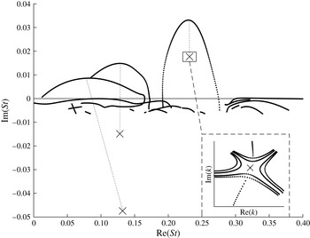
More interesting results were found for modes with non-zero azimuthal wavenumbers. Figure 18 shows the complex
 $\unicode[STIX]{x1D714}$
plane (expressed in terms of the Strouhal number,
 $St$
) with temporal and spatio-temporal results for a typical slice in the main cone of the cyclone separator (
 $Sw=5.1$
,
 $D_{e}/D=0.26$
).
Complex
 $\unicode[STIX]{x1D714}$
plane (non-dimensionalised as Strouhal numbers) showing temporal stability curves
 $\unicode[STIX]{x1D714}(k_{r})$
(dotted lines) and saddle points for which
 $\text{d}\unicode[STIX]{x1D714}/\text{d}k=0$
(crosses) for an azimuthal wavenumber of
 $m=-1$
. For this slice, only one of the saddle points is absolutely unstable. We confirmed that these are valid
 $k+/k-$
pinch points (the complex
 $k$
plane is shown in the inset with saddle point contours traced out). The location of the slice is shown as slice 1 in figure 19.

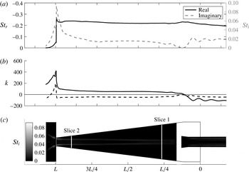
We observe that there are numerous temporally unstable modes. Only one of these has an unstable saddle point associated with it. This absolute instability is found to exist along the entire length of the cyclone cone and is also present in the vortex finder and outlet tube of the flow. Figure 19 shows the axial variation of the saddle point frequency and wavenumber as well as the shape of the associated eigenfunction in the radial direction. The real component of frequency remains mostly constant within the conical part of the cyclone. The growth rate (imaginary frequency) of the mode is maximum at the narrow tip of the cone.
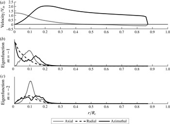
Axial variation of the absolutely unstable mode with azimuthal wavenumber
 $m=-1$
. The variations of real and imaginary frequencies (a) and wavenumbers (b) are shown. The axial locations are aligned with the cyclone shown in (c). Contours within the cyclone show the velocity perturbation magnitude multiplied by the growth rate. It can be observed that the real frequency and radial position of the mode remain nearly constant along the entire length of the cyclone cone.

The sign of the real part of the axial wavenumber
 $\text{Re}(k_{0})$
is opposite to that of
 $m$
inside the main body of the cyclone. The frequency,
 $\text{Re}(\unicode[STIX]{x1D714}_{0})$
, has the same sign as
 $m$
. The wave crests rotate (in time) in the same direction as the flow, but wind (in space) in the opposite direction. Loiseleux et al. (Reference Loiseleux, Chomaz and Huerre1998) found that negative azimuthal wavenumbers defined the absolutely unstable behaviour of an ideal Rankine vortex with axial flow, and their sign convention is in agreement with these observations of the cyclone flow (i.e.
 $m<0$
when
 $\text{Re}(k)>0$
). In the vortex finder, the sign of
 $\text{Re}(k)$
changes to be the same as
 $m$
. Hence, the oscillation is spiralling in the opposite sense, which suggests that there is a different mode of instability in the vortex finder.
There is a rapid decrease in the saddle point frequency in the dust collector region of the flow. In this area, the swirling flow is no longer confined and expands into the larger diameter as a swirling jet and then recirculates back on itself (see figure 6). The mode shape in figure 19 follows the path of the expanding jet into the dust collector. The drop in saddle point frequency is found to be proportional to the reduction in angular velocity of this jet as it grows. However, in this region, the flow exhibits a departure from the assumptions of parallel flow, as there is a significant radial velocity.
5.3 Azimuthal wavenumber
 $m=-2$

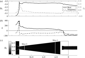
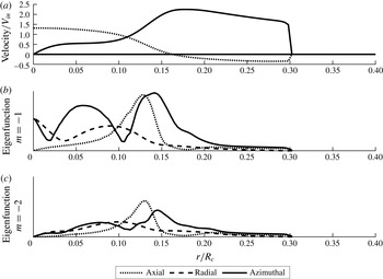
The same behaviour is observed for larger non-zero azimuthal wavenumbers with a single dominant absolute instability. Figure 20 shows the axial variations of the
 $m=-2$
saddle point. The shape of the eigenfunction is similar to the
 $m=-1$
mode and the peak growth rate is also at the tip of the cone. The growth rate of the
 $m=-2$
mode is double that of
 $m=-1$
at the cone tip, which indicates that this mode may dominate here. The magnitude of the growth rate decreases significantly towards the top of the cone, and becomes stable, resulting in this region being convectively unstable rather than absolutely unstable. The sense of the double-helix rotation is the same as for
 $m=-1$
.
As figure 19 but with
 $m=-2$
.

From the visualisation of the flow using high-speed photography, an
 $m=-2$
oscillation with a precessing double vortex core is observed at the narrow tip of the cyclone (see figure 10
c). This feature is only observed at the narrow cone tip, which coincides with the region of absolute instability for
 $m=-2$
in the local stability model.
5.4 Comparison with visualisation and anemometry
It has been shown that a pocket of absolute instability can lead to the development of a self-sustained global mode of oscillation for a system (Huerre & Monkewitz Reference Huerre and Monkewitz1990). In the case of the cyclone, there are absolute instabilities present throughout the flow. Visualisation using high-speed photography reveals the presence of precessing motions inside the cyclone. At the top, these motions have the form of an
 $|m|=1$
azimuthal wavenumber oscillation. At the tip, the motions are dominated by an
 $|m|=2$
oscillation with a double vortex core. In between these two ends of the cyclone, there is a transition region where there is no single dominant frequency component to the vortex core motions.
The local stability results show that an
 $|m|=1$
fluctuation is absolutely unstable along the entire length of the cyclone cone, but the frequency of this unstable mode changes gradually as we move from the top to the tip of the cone. Hot-wire anemometry measurements at the top and tip of the cone also find that the Strouhal number of fluctuations is higher at the tip than at the top of the cone.
The stability results predict an absolutely unstable
 $|m|=2$
mode at the tip of the cone only. Its growth rate surpasses that of the
 $|m|=1$
mode at the same location. The visualisation of the flow shows that the double-core phenomenon is only seen at the cone tip, which coincides with the region of strong absolute instability and large positive growth rate. This explains why the phenomenon is only seen at this end of the cyclone. The growth rate rapidly decreases away from the cone tip, with the saddle point frequency becoming stable.
In the mid-section of the cyclone, no discernible precession is observed with either high-speed video or hot-wire measurements. This, combined with the prediction of helical structures with different directions of rotation at each end of the cone, suggests that the oscillations observed at each end are the result of two separate unstable regions of the flow, and there is a transition between them at which neither mode is dominant.
5.5 Flow rate variations
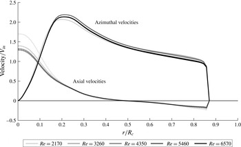
Figure 21 shows the changes in mean velocity for variations in the Reynolds number
 $Re$
(by changing the flow rate
 $Q$
) from five RANS simulations. The shape of the mean flow remains the same for all flow rates, and the magnitudes are linearly proportional to
 $V_{in}$
. Therefore, it is expected that the same oscillation mechanism exists for all flow rates as it is driven by inflection points in the mean flow, which are present in all cases. The lowest-
 $Re$
case shows a small divergence from this collapse, with weaker swirl and stronger axial flow relative to the other cases.
Axial (dotted lines) and azimuthal (solid lines) mean velocities for variations in the volumetric flow rate from slice 1 of figures 19 and 20. The operating points for each case have been non-dimensionalised as the Reynolds number,
 $Re$
. The internal velocities scale proportionally with the flow rate as the velocities collapse when non-dimensionalised by the inlet velocity. At low values of
 $Re$
, the balance of swirl and axial velocities changes, with less swirl being developed and a tighter stronger axial jet up the centre.

Figure 22 shows the variation in absolute frequency with flow rate for both
 $|m|=1$
and
 $|m|=2$
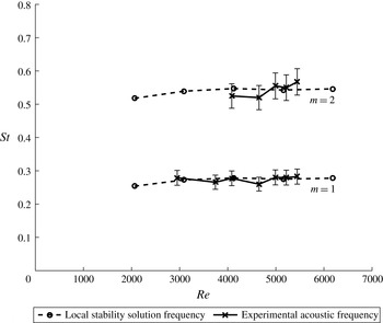
taken from slice 1. These results are compared with the frequencies of the acoustic hum measured experimentally (Grimble & Agarwal Reference Grimble and Agarwal2015). The hum has both a fundamental frequency and a second, approximately harmonic, peak that were identified in the experiments. The absolute instabilities appear to asymptote to a constant Strouhal number at high Reynolds numbers, which matches the hum frequencies from experiment.


This behaviour matches other studies of the precessing vortex core such as the work of Yazdabadi et al. (Reference Yazdabadi, Griffiths and Syred1994a ), where the Strouhal number was measured across a wide range of Reynolds numbers. The oscillation frequency increased with the Reynolds number, but tended towards a constant value at high Reynolds numbers. The local stability results capture this behaviour, and it can be seen that the lowest Reynolds number has a slightly lower Strouhal number, but then asymptotes towards a constant value as the flow rate is increased.
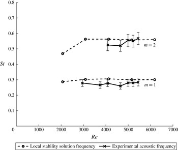
As figure 22 but at slice 2. The frequencies do not match as well for
 $|m|=1$
.

Figure 23 shows the comparison of local stability and acoustic results at slice 2 from figures 19 and 20. In this case, the local stability results for
 $|m|=1$
overpredict the acoustic frequency. The frequency ratio between
 $|m|=1$
and
 $|m|=2$
is significantly less than 1 : 2, as expected.
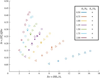
The Strouhal number of the
 $|m|=1$
mode as a function of the swirl number: local stability solutions, filled symbols; measurements from acoustic experiments, unfilled symbols. The collapse shown has been achieved using a fluid density of 1.0 kg m
 $^{-3}$
to scale the volumetric flow rate, which is consistent with the conditions at the core of the vortex. Use of this value of the density provides a good agreement between the linear instability predictions and acoustic experiments.

5.6 Swirl number variations
A range of different inlet and outlet areas have been modelled with RANS simulations to directly compare the variation of swirl number with the acoustic experiment results. The inlet and outlet areas are examined independently with five variations of each while keeping the other parameters constant. This set of simulations provided data to compare with the acoustic hum frequencies.
All of the cyclones exhibited the same behaviour, with a single dominant absolute instability for non-zero azimuthal wavenumbers, as has been described in the previous sections. Figure 24 shows the absolute frequencies,
 $\unicode[STIX]{x1D714}_{0}$
, for
 $|m|=1$
, taken from slice 1 in figure 19 in each case, compared with the acoustic measurements of Grimble & Agarwal (Reference Grimble and Agarwal2015). The frequencies from the local analysis follow the same trends for both inlet and outlet area changes and closely match the experimentally measured hum frequencies for the same geometry. This strongly links the instability of the flow to the acoustic noise.
Scaling of the simulation results was carried out by choosing a density by which to scale the volumetric flow rate from the mass flow of the simulation. The simulations model compressible flow using ideal gas laws, such that the density varies throughout the flow. There are significant changes in density between the vortex core and the walls of the cyclone, with changes ranging from 1.0 kg m
 $^{-3}$
at the centre up to 1.1 kg m
 $^{-3}$
at the outer wall. This 10 % drop in density at the core is primarily due to the low pressure resulting from the strong swirl. Based on the fact that the observed oscillation structures are at the core, we have used the lower density to scale the volumetric flow values used to calculate the Strouhal numbers in figure 24.
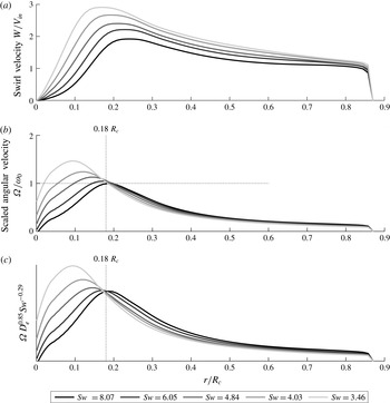
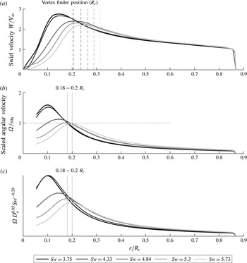
The nature of the scaling between acoustics and stability analysis can be examined further by comparing the swirl velocity profiles resulting from shifts in the swirl number. Figure 25 shows the swirl velocity profiles at slice 1 for the simulations with different inlet areas. By converting these swirl velocities into angular velocities, we can directly compare them with the frequencies of the predicted instabilities. It can be seen that the angular velocity of the flow matches the absolute frequency at approximately the same radius in each case.
The acoustic experiments carried out by Grimble & Agarwal (Reference Grimble and Agarwal2015) produced an empirical non-dimensional model for the oscillation frequencies:
 $$\begin{eqnarray}St\propto Sw^{-0.71}\left(\frac{D_{e}}{D}\right)^{2.15}.\end{eqnarray}$$
By using the
 $Sw$
and
 $St$
scalings it is possible to rearrange (5.1) to create a functional group that collapses to a constant, which can be applied to any frequency based unit, such as the angular velocity:
 $$\begin{eqnarray}\unicode[STIX]{x1D6FA}{D_{e}}^{0.85}Sw^{0.29}\propto \text{const.}\end{eqnarray}$$
This collapse is applied to the angular velocity in figure 25(c), where there is a single position where a collapse occurs, which corresponds to a radius of
 $0.18R$
. This collapse indicates that the non-dimensional equation isolates both the magnitude and the location of vortex oscillations.
Swirl velocity (a) and angular velocity (b) profiles as a function of radius for swirl number variations resulting from changes in the effective inlet area. The angular velocity (
 $\unicode[STIX]{x1D6FA}$
) has been scaled by the real frequency of the absolute instability predicted for each flow profile (
 $\unicode[STIX]{x1D714}_{0}$
) to show where they coincide (
 $\unicode[STIX]{x1D6FA}/\unicode[STIX]{x1D714}_{0}=1$
). It is noted that the frequencies coincide with the angular velocity of the flow at approximately the same radius for all cases. This corresponds to a radius of
 $0.18R_{c}$
. The selected frequency location is close to the boundary between the inner and outer vortex regimes. Panel (c) applies the empirical frequency model from Grimble & Agarwal (Reference Grimble and Agarwal2015) to the swirl velocity profiles and shows that there exists a collapse at the same radial location.

Figure 26 shows the swirl velocity profiles resulting from outlet area changes. Again, a collapse is observed close to the same position as in figure 25. In this case, the range of positions varies between
 $0.18R_{c}$
and
 $0.2R_{c}$
. We note that this radius increases with the vortex finder radius, but a significant shift in
 $R_{e}$
only results in a small change in the collapse position. These results suggest that there may be a critical radius at which the oscillations within the vortex core couple into the angular velocity of the vortex. This position is independent of the swirl number and is slightly modified by the outlet radius
 $R_{e}$
. It is also of note that this location remains mostly constant, even though the location of the transition between forced and free vortex regimes shifts significantly with both the outlet size and the inlet area. The position of this collapse is also consistent with the hot-wire anemometry measurements in § 4.3, where oscillations were detected for radii less than
 $0.2R_{c}$
.
As figure 25 but with swirl number variations from changes in the outlet diameter. The same approximate location (between 0.18 and 0.2
 $R_{c}$
) is found for the angular velocity collapse and frequency match for this set of parameter changes.

5.7 Physical mechanisms
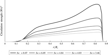
Figure 27 shows how the square of the circulation changes with the radius for the flow profiles shown in figure 25. Within the main body of the flow, this quantity increases with
 $r$
, indicating that the flow is centrifugally stable according to Rayleigh’s criterion (Rayleigh 1916). However, within the boundary layer, localised centrifugal instabilities can develop in the form of Görtler vortices (Saric Reference Saric1994). These instabilities are at much higher frequencies than those observed here and are not relevant to the present study.
Rayleigh’s centrifugal stability criterion, showing circulation strength as a function of radius for the cyclone flow profiles in figure 25.

While centrifugal instability mechanisms may be confined to the near-wall region, the oscillation structures observed in this study are within the vortex core. The solid-body rotation of the core of a Rankine vortex is able to act as a waveguide for neutrally stable inertial waves (Saffman Reference Saffman1992). Examination of the eigenfunctions of the predicted absolute instabilities (figures 28 and 29) shows that the fluctuations are focused within this solid-body core. The axial eigenfunction has the highest magnitude at the inflection point in the axial velocity profile (
 $r/R_{c}\approx 0.1$
). The shear layer and inertial waves couple together to select the frequency at the edge of this core region, as was shown by the absolute frequency and angular velocity comparisons in figure 25.


This coupling between the shear layer instability and the inertial waves propagating along the vortex core has been studied in detail by Loiseleux et al. (Reference Loiseleux, Chomaz and Huerre1998) and Gallaire & Chomaz (Reference Gallaire and Chomaz2003). In the case of the cyclone separator, changes in the inlet and outlet areas vary the size of the vortex core. This varies the frequency of the waves predicted within the vortex core by the local stability analysis. The application of the empirical model for inlet and outlet area changes to the swirl velocity profiles (figures 25 and 26) shows that this model has captured aspects of the flow physics that lead to oscillations and highlights a location in the flow that plays a role in mode selection.
The experimental observations showed no clear oscillations in the mid-section of the cone. As the flow enters the vortex finder, the core is suddenly confined, which may result in interactions between the helical waves within the vortex core and the walls. We note that the vortex finder is approximately the same size as the vortex core, where the oscillations have been observed. The sudden confinement of a supercritical swirling flow could also result in vortex breakdown within the vortex finder. The resulting recirculation structures from vortex breakdown have been shown to be unstable to helical waveforms and could generate noise.
At the bottom of the cone near the cone tip, a similar confinement of the vortex is observed, but in this case the contraction is gradual. At the cone tip, the vortex core is directly adjacent to the wall, where the swirling boundary layer may contain strong Görtler vortices. The boundary layer vortex structures may disrupt the core oscillations, which generate the oscillations observed here and the acoustic hum. In addition, the sudden expansion of the vortex into the dust collector at the tip of the cone could produce a precessing flow structure as the vortex breaks down, which could lead to noise radiating from the bottom of the cyclone. This is similar to the precession and recirculation structures observed in swirl burners (Syred Reference Syred2006).
6 Conclusions
The cyclone separator flow is absolutely unstable to disturbances with non-zero azimuthal wavenumber, i.e. helical modes. From visualisation, the dominant mode at the top of the cyclone is an
 $m=1$
azimuthal mode. At the cone tip,
 $m=2$
is dominant. The peak unstable growth rate for both
 $m=1$
and
 $m=2$
is at the narrow tip of the cyclone.
Comparison with acoustic measurements shows that the
 $m=1$
absolute instability frequency near the top of the cone matches the observed acoustic hum. The behaviour of both phenomena is the same for variations of flow rate and swirl number. The application of local stability analysis to the cyclone separator shows that hydrodynamic instability is the source of the acoustic noise. The results show that there is a significant coherent oscillation of the flow, which has its source in the strong shear near the vortex core coupled with inertial waves induced by the swirling system.
The local stability analysis predictions and mode shapes agree with the visualisation of the oscillations in water and hot-wire anemometry results. Furthermore, it has been possible to observe how the equation of an empirically derived non-dimensional model of acoustic noise picks out the location and magnitude of the vortex core oscillations. This adds to the strength of this model by imparting information about the physical flow structures within the cyclone separator and how these can result in the observed oscillations.
This provides a validated example for the application of local stability analysis to a real swirling flow and offers a means to study the mechanisms behind unsteadiness in the flow. This understanding can help to guide the design of potential flow control systems. To further develop this work, the assumptions of parallel flow could be removed by considering the global stability of the system. The local analysis reveals a range of frequencies that are excited at different axial locations. The study within this paper has relied on the observation that the change in absolute frequency is small with length, and the same mode shape exists throughout the cone. A global analysis would show whether a single particular frequency and location are critical for the unsteadiness and result in the discrete hum frequency that is observed.
Acknowledgements
We gratefully acknowledge Dyson Ltd. for funding this project. We are grateful to F. Nicolas’ group at Dyson for their generous technical and administrative support. We would also like to thank J. Lamb from Dyson and A. Dowling from Cambridge for many useful discussions, and J. Hazlewood for his help with setting up and manufacturing the experimental rig.