1 Introduction
The energy transfer in the physical and wavenumber spaces is important in understanding turbulent flows and in constructing turbulence models. For homogeneous isotropic turbulence, the energy spectrum, which is the Fourier transform of the two-point velocity correlation, is commonly used to describe the scale dependence of the turbulent fluctuations and the energy transfer in the wavenumber space. The energy cascade from low to high wavenumbers has been studied in detail, and several closure theories have been proposed (Frisch Reference Frisch1995). However, for inhomogeneous turbulence, one-point statistical quantities are employed such as the turbulent kinetic energy. The energy production, dissipation and transfer in the physical space are described using one-point closure models (Pope Reference Pope2000). It is very complex to treat two-point quantities in inhomogeneous turbulence models.
In order to improve turbulence models, a few attempts have been made to utilize the energy spectrum for inhomogeneous turbulence. In a statistical theory called the two-scale direct interaction approximation (Yoshizawa Reference Yoshizawa1984, Reference Yoshizawa1998), fast and slow variables for space coordinates were defined. The Fourier transform with respect to the fast variable was performed to utilize the closure theory for homogeneous isotropic turbulence (Kraichnan Reference Kraichnan1959; Leslie Reference Leslie1973), whereas the slow variable was used to describe the inhomogeneity of turbulent fields. In a turbulence model developed by Schiestel (Reference Schiestel1987), multi-scale turbulent kinetic energies were introduced by dividing the energy spectrum into several parts at different wavenumbers. The transport equations for the kinetic energies at different scales were used to improve the prediction of turbulent flows (Schiestel & Dejoan Reference Schiestel and Dejoan2005; Chaouat & Schiestel Reference Chaouat and Schiestel2005). To describe the energy transfer not only in the physical space but also in the wavenumber space must be useful in improving inhomogeneous turbulence models. However, in these approaches, the Fourier transform and the energy spectrum were introduced in an approximate manner and the procedure needs to be justified physically.
If the velocity field in inhomogeneous turbulence is statistically homogeneous in some directions, the Fourier transform in those directions can be performed in a rigorous manner. For example, turbulent channel flows have been examined using the energy spectrum in the streamwise and spanwise directions (Domaradzki et al. Reference Domaradzki, Liu, Härtel and Kleiser1994; Dunn & Morrison Reference Dunn and Morrison2003; Bolotnov et al. Reference Bolotnov, Lahey, Drew, Jansen and Oberai2010). Recently, Lee & Moser (Reference Lee and Moser2015) studied the scale dependence of the dynamics of the Reynolds stress by examining its transport equation in turbulent channel flows. Mizuno (Reference Mizuno2016) evaluated the spectral energy budget equation to reveal the scale dependence of the energy transport. However, the Fourier transform cannot be applied in the inhomogeneous direction for general turbulent flows.
Instead of the energy spectrum, the second-order structure function
 $\langle \unicode[STIX]{x1D6FF}u_{i}^{2}(\boldsymbol{x},\boldsymbol{r})\rangle$
(where
 $\unicode[STIX]{x1D6FF}u_{i}(\boldsymbol{x},\boldsymbol{r})=u_{i}^{\prime }(\boldsymbol{x}+\boldsymbol{r})-u_{i}^{\prime }(\boldsymbol{x})$
and
 $u_{i}^{\prime }(\boldsymbol{x})$
is the velocity fluctuation) and the two-point velocity correlation
 $Q_{ii}(\boldsymbol{x},\boldsymbol{r})(=\langle u_{i}^{\prime }(\boldsymbol{x})u_{i}^{\prime }(\boldsymbol{x}+\boldsymbol{r})\rangle )$
in the physical space can be used to approximately describe the kinetic energy of eddies of length scale
 $r(=|\boldsymbol{r}|)$
. For homogeneous isotropic turbulence, the Kármán–Howarth equation and Kolmogorov’s equation were formulated using the two-point correlation and the structure function, respectively, and the latter equation can be derived from the former (Frisch Reference Frisch1995). Several attempts have been made to extend these equations to inhomogeneous turbulence (Danaila et al.
Reference Danaila, Anselmet, Zhou and Antonia2001; Hill Reference Hill2002; Marati, Casciola & Piva Reference Marati, Casciola and Piva2004; Davidson Reference Davidson2004; Danaila et al.
Reference Danaila, Krawczynski, Thiesset and Renou2012; Cimarelli, De Angelis & Casciola Reference Cimarelli, De Angelis and Casciola2013; Hamba Reference Hamba2015; Cimarelli et al.
Reference Cimarelli, De Angelis, Jiménez and Casciola2016). Danaila et al. (Reference Danaila, Anselmet, Zhou and Antonia2001) examined the turbulent diffusion and dissipation terms in the centre of a channel flow, and proposed a generalized form of Kolmogorov’s equation. Hill (Reference Hill2002) theoretically derived the exact transport equation for the structure function in inhomogeneous turbulence, and discussed opportunities for investigations using the equation. Marati et al. (Reference Marati, Casciola and Piva2004) evaluated the structure function equation using direct numerical simulation (DNS) data of a turbulent channel flow. They investigated a scale-by-scale balance for the turbulent fluctuations to describe the dynamics of turbulence in different regions of a channel flow. Cimarelli et al. (Reference Cimarelli, De Angelis and Casciola2013) and Cimarelli et al. (Reference Cimarelli, De Angelis, Jiménez and Casciola2016) examined the energy flux occurring in the scale space and in the physical space in turbulent channel flows. An interesting behaviour of the energy flux was observed where the inverse energy cascade plays a central role. Danaila et al. (Reference Danaila, Krawczynski, Thiesset and Renou2012) developed a scale-by-scale kinetic energy budget equation for inhomogeneous and anisotropic turbulence using the structure function. They examined experimental data obtained in a multiple-opposed-jets flow to validate the energy equation and to clarify the anisotropic energy transfer. Instead of the structure function itself, Davidson (Reference Davidson2004) defined the turbulent energy density in the scale space using the
 $r$
derivative of the structure function. In that study, the energy density was compared with the structure function in homogeneous isotropic turbulence and wall turbulence (Davidson & Pearson Reference Davidson and Pearson2005; Davidson, Nickels, & Krogstad Reference Davidson, Nickels and Krogstad2006). Using the two-point velocity correlation, Hamba (Reference Hamba2015) proposed an expression for the turbulent energy density in the scale space and examined the energy transfer in a turbulent channel flow.
Similar to the energy spectrum, the energy density in the scale space is required to satisfy the following properties (Davidson Reference Davidson2004). First, the energy density should be non-negative. Second, the integral of the energy density over all scales should equal the turbulent kinetic energy itself. The structure function is non-negative, but its integral does not equal the turbulent kinetic energy (instead, the structure function itself tends to twice the energy as
 $r\rightarrow \infty$
). In contrast, Davidson (Reference Davidson2004) introduced the gradient of the structure function as the energy density which satisfies the second property, but the quantity is not necessarily non-negative. The same holds for the energy density proposed by Hamba (Reference Hamba2015). Thus far, no expression has been found that satisfies both properties. In the present work, we propose a new expression for the energy density in the scale space by using the integral of the velocity correlation with a filter function. The new expression is non-negative in the scale space of the homogeneous direction and satisfies the two properties. We expect that the new expression for the energy density can be used to properly describe the energy transfer in the scale space and to improve turbulence models.
This paper is organized as follows. In § 2, we introduce a new expression for the energy density in the scale space, and we derive its transport equation for inhomogeneous turbulence. In § 3, we evaluate the energy density and its transport equation using DNS data of homogeneous isotropic turbulence. We compare profiles of the energy density in the scale space with those of the energy spectrum in the wavenumber space. In § 4, we evaluate the energy density using DNS data of a turbulent channel flow to compare the results between the previous and new expressions. Then, to investigate the energy cascade, we examine the transport equation for the energy density, including the energy fluxes in the scale space and in the physical space. Finally, we conclude the paper in § 5.
2 Turbulent energy density in scale space
Before introducing the turbulent energy density in the scale space, we describe the transport equations for the turbulent kinetic energy in the physical space and in the wavenumber space, respectively. The velocity is divided into the mean and fluctuating parts as follows:
 $$\begin{eqnarray}u_{i}=U_{i}+u_{i}^{\prime },\quad U_{i}\equiv \langle u_{i}\rangle ,\end{eqnarray}$$
where
 $\langle \;\rangle$
denotes ensemble averaging. The turbulent kinetic energy
 $K(=\langle u_{i}^{\prime 2}\rangle /2)$
is an important quantity representing the intensity of the turbulent fluctuations.
For decaying homogeneous isotropic turbulence, the transport equation for
 $K$
is given by
 $$\begin{eqnarray}\frac{\unicode[STIX]{x2202}K}{\unicode[STIX]{x2202}t}=-\unicode[STIX]{x1D700}.\end{eqnarray}$$
The energy dissipation rate
 $\unicode[STIX]{x1D700}$
is defined as
 $$\begin{eqnarray}\unicode[STIX]{x1D700}=\unicode[STIX]{x1D708}\left\langle \frac{\unicode[STIX]{x2202}u_{i}^{\prime }}{\unicode[STIX]{x2202}x_{j}}\frac{\unicode[STIX]{x2202}u_{i}^{\prime }}{\unicode[STIX]{x2202}x_{j}}\right\rangle ,\end{eqnarray}$$
where
 $\unicode[STIX]{x1D708}$
is the kinematic viscosity, and the summation convention is used for repeated indices. The dissipation rate should be
 $(\unicode[STIX]{x1D708}/2)\langle (\unicode[STIX]{x2202}u_{i}^{\prime }/\unicode[STIX]{x2202}x_{j}+\unicode[STIX]{x2202}u_{j}^{\prime }/\unicode[STIX]{x2202}x_{i})^{2}\rangle$
in a rigorous sense. However, both expressions are equal to each other for homogeneous turbulence and their difference is negligibly small for high-Reynolds-number inhomogeneous turbulence. The expression (2.3) is often used for turbulence models; one of the reason is that the expression leads to a simple viscous diffusion term for inhomogeneous turbulence as will be seen in (2.12). Therefore, we adopt (2.3) in the present analysis. Because of the homogeneity, the turbulent kinetic energy is a function of time only; over time, the energy decays monotonically owing to the viscous effect. The equation is too simple to examine the status of the turbulent field. To describe the turbulent field in more detail, the energy spectrum
 $E(k)(=2\unicode[STIX]{x03C0}k^{2}\hat{Q}_{ii}(\boldsymbol{k}))$
is often introduced, where
 $\hat{Q}_{ii}(\boldsymbol{k})$
is the three-dimensional Fourier transform of the velocity correlation
 $Q_{ii}(\boldsymbol{r})$
. The energy spectrum
 $E(k)$
represents the energy density in the wavenumber space and satisfies the following properties:
 $$\begin{eqnarray}\displaystyle E(k)\geqslant 0, & & \displaystyle\end{eqnarray}$$
 $$\begin{eqnarray}\displaystyle K=\int _{0}^{\infty }\text{d}kE(k). & & \displaystyle\end{eqnarray}$$
The energy spectrum
 $E(k)$
contains information not only on the intensity but also on the scale dependence of the turbulent fluctuations; it is approximately considered the kinetic energy of eddies of size
 $\unicode[STIX]{x03C0}/k$
. The transport equation for
 $E(k)$
is written as
 $$\begin{eqnarray}\frac{\unicode[STIX]{x2202}}{\unicode[STIX]{x2202}t}E(k)=-\unicode[STIX]{x1D700}(k)+T(k).\end{eqnarray}$$
The dissipation term
 $\unicode[STIX]{x1D700}(k)$
and the energy transfer term
 $T(k)$
are defined as
 $$\begin{eqnarray}\displaystyle & \displaystyle \unicode[STIX]{x1D700}(k)=2\unicode[STIX]{x1D708}k^{2}E(k), & \displaystyle\end{eqnarray}$$
 $$\begin{eqnarray}\displaystyle & \displaystyle T(k)=2\unicode[STIX]{x03C0}k^{2}\int \int \text{d}\boldsymbol{p}\,\text{d}\boldsymbol{q}S(\boldsymbol{k},\boldsymbol{p},\boldsymbol{q}), & \displaystyle\end{eqnarray}$$
respectively, where
 $S(\boldsymbol{k},\boldsymbol{p},\boldsymbol{q})$
is the triple velocity correlation (its detailed expression is omitted here). The transfer term
 $T(k)$
can be rewritten as
 $$\begin{eqnarray}T(k)=-\frac{\unicode[STIX]{x2202}}{\unicode[STIX]{x2202}k}\unicode[STIX]{x1D6F1}(k),\quad \unicode[STIX]{x1D6F1}(k)=\int _{k}^{\infty }\text{d}k^{\prime }T(k^{\prime }).\end{eqnarray}$$
The energy flux
 $\unicode[STIX]{x1D6F1}(k)$
represents the flow of the turbulent kinetic energy in the wavenumber space. Using the energy spectrum and its transport equation, we can examine the energy cascade from low to high wavenumbers. When each term in (2.6) is integrated from
 $k=0$
to
 $\infty$
, (2.6) reduces to the
 $K$
equation given by (2.2). The transfer term disappears in the
 $K$
equation because
 $$\begin{eqnarray}\int _{0}^{\infty }\text{d}kT(k)=0.\end{eqnarray}$$
For inhomogeneous turbulence, the turbulent kinetic energy is a function of not only time but also position. The transport equation for
 $K$
in the physical space is given by
 $$\begin{eqnarray}\frac{\text{D}K}{\text{D}t}=P-\unicode[STIX]{x1D700}+D,\end{eqnarray}$$
where
 $\text{D}/\text{D}t=\unicode[STIX]{x2202}/\unicode[STIX]{x2202}t+U_{i}\unicode[STIX]{x2202}/\unicode[STIX]{x2202}x_{i}$
. The production term
 $P$
and the diffusion term
 $D$
are defined as
 $$\begin{eqnarray}P=-\langle u_{i}^{\prime }u_{j}^{\prime }\rangle \frac{\unicode[STIX]{x2202}U_{i}}{\unicode[STIX]{x2202}x_{j}},\quad D=-\frac{\unicode[STIX]{x2202}\unicode[STIX]{x1D6F7}_{j}}{\unicode[STIX]{x2202}x_{j}},\quad \unicode[STIX]{x1D6F7}_{j}=\left\langle \frac{1}{2}u_{i}^{\prime 2}u_{j}^{\prime }\right\rangle +\langle p^{\prime }u_{j}^{\prime }\rangle -\unicode[STIX]{x1D708}\frac{\unicode[STIX]{x2202}K}{\unicode[STIX]{x2202}x_{j}},\end{eqnarray}$$
respectively. The diffusion term
 $D$
is written in the divergence form, and
 $\unicode[STIX]{x1D6F7}_{j}$
represents the energy flux in the
 $j$
th direction in the physical space; it consists of three parts: turbulent diffusion, pressure diffusion and viscous diffusion. The processes described by (2.11) for inhomogeneous turbulence are complex compared to (2.2) for homogeneous isotropic turbulence. Nevertheless, (2.11) does not contain information on the scale dependence of the turbulent fluctuations, and more insight is needed for turbulent flows. In fact, for a turbulent channel flow, the Fourier transform is performed in the homogeneous streamwise and spanwise directions to analyse the energy transfer in the wavenumber space. However, it is not always possible to perform the Fourier transform for general inhomogeneous turbulent flows.
Instead of the energy spectrum in the wavenumber space, the energy density in the scale space must be useful for inhomogeneous turbulence. The energy density
 $E(\boldsymbol{x},r)$
in the scale space is a function of not only position
 $\boldsymbol{x}$
but also length scale
 $r$
, and should satisfy the following properties:
 $$\begin{eqnarray}\displaystyle & \displaystyle E(\boldsymbol{x},r)\geqslant 0, & \displaystyle\end{eqnarray}$$
 $$\begin{eqnarray}\displaystyle & \displaystyle K(\boldsymbol{x})=\int _{0}^{\infty }\text{d}rE(\boldsymbol{x},r), & \displaystyle\end{eqnarray}$$
as in the case of (2.4) and (2.5) for the energy spectrum (Davidson Reference Davidson2004). Although several energy densities and scale energies have been proposed so far, no quantity satisfies both properties. For example, Hill (Reference Hill2002) derived the transport equation for the second-order structure function; it has been used to investigate the transport of the scale energy in a channel flow in detail (Marati et al. Reference Marati, Casciola and Piva2004). The structure function satisfies (2.13) but not (2.14); that is, it is non-negative, but its integral does not equal the turbulent kinetic energy. Davidson (Reference Davidson2004) proposed the energy density using the structure function as follows:
 $$\begin{eqnarray}E(\boldsymbol{x},r)=-\frac{3}{8}r^{2}\frac{\unicode[STIX]{x2202}}{\unicode[STIX]{x2202}r}\frac{1}{r}\frac{\unicode[STIX]{x2202}}{\unicode[STIX]{x2202}r}\langle (\unicode[STIX]{x0394}u)^{2}\rangle ,\end{eqnarray}$$
where
 $\unicode[STIX]{x0394}u=u_{x}(\boldsymbol{x}+r\boldsymbol{e}_{x})-u_{x}(\boldsymbol{x})$
. Conversely, it satisfies (2.14) but not (2.13). The same holds for the energy density proposed by Hamba (Reference Hamba2015) using the two-point velocity correlation as follows:
 $$\begin{eqnarray}E(\boldsymbol{x},r)=-\frac{1}{2}\frac{\unicode[STIX]{x2202}}{\unicode[STIX]{x2202}r}Q_{ii}(\boldsymbol{x},\boldsymbol{r}).\end{eqnarray}$$
In (2.15) and (2.16), the derivative with respect to
 $r$
is introduced so that
 $E(\boldsymbol{x},r)$
can satisfy (2.14); instead, they are not necessarily non-negative.
In this work, by improving (2.16), we seek to determine the energy density in the following form:
 $$\begin{eqnarray}E(r)=-\frac{\unicode[STIX]{x2202}}{\unicode[STIX]{x2202}r}E_{{>}}(r),\end{eqnarray}$$
with the conditions
 $$\begin{eqnarray}E_{{>}}(0)=K,\quad E_{{>}}(\infty )=0,\end{eqnarray}$$
where the dependence of the energy density on position
 $\boldsymbol{x}$
is omitted for simplicity. Because the energy
 $E_{{>}}(r)$
is written as
 $$\begin{eqnarray}E_{{>}}(r)=\int _{r}^{\infty }\text{d}r^{\prime }E(r^{\prime }),\end{eqnarray}$$
it represents the kinetic energy of eddies whose sizes are equal to or greater than
 $r$
, and the energy density given by (2.17) with (2.18) automatically satisfies (2.14). We then seek an expression for
 $E_{{>}}(r)$
that leads to non-negative
 $E(r)$
.
Here, we consider the fact that the energy spectrum
 $E(k)$
satisfies both (2.4) and (2.5). It suggests that
 $\hat{Q}_{ii}(\boldsymbol{k})$
can be utilized for
 $E_{{>}}(r)$
in homogeneous turbulence where the Fourier transform is possible. We consider the one-dimensional Fourier transform of the velocity correlation
 $Q_{ii}(\unicode[STIX]{x1D709})$
(
 $=Q_{ii}(\boldsymbol{x},\unicode[STIX]{x1D743})$
) for homogeneous isotropic turbulence, which is given by
 $$\begin{eqnarray}\hat{Q}_{ii}(k)=\frac{1}{2\unicode[STIX]{x03C0}}\int _{-\infty }^{\infty }\text{d}\unicode[STIX]{x1D709}Q_{ii}(\unicode[STIX]{x1D709})\exp (-\text{i}k\unicode[STIX]{x1D709}).\end{eqnarray}$$
Making use of
 $\hat{Q}_{ii}(k)$
with
 $k=\unicode[STIX]{x03C0}/r$
, we can define the following energy density
 $$\begin{eqnarray}E(r)=\frac{\unicode[STIX]{x03C0}}{r^{2}}\hat{Q}_{ii}\left(\frac{\unicode[STIX]{x03C0}}{r}\right),\end{eqnarray}$$
and
 $$\begin{eqnarray}E_{{>}}(r)=\int _{r}^{\infty }\text{d}r^{\prime }\frac{\unicode[STIX]{x03C0}}{{r^{\prime }}^{2}}\hat{Q}_{ii}\left(\frac{\unicode[STIX]{x03C0}}{r^{\prime }}\right).\end{eqnarray}$$
The energy
 $E_{{>}}(r)$
satisfies the conditions given by (2.18) as follows:
 $$\begin{eqnarray}E_{{>}}(0)=\int _{0}^{\infty }\text{d}r\frac{\unicode[STIX]{x03C0}}{r^{2}}\hat{Q}_{ii}\left(\frac{\unicode[STIX]{x03C0}}{r}\right)=\int _{-\infty }^{\infty }\text{d}k\frac{1}{2}\hat{Q}_{ii}(k)=K,\quad E_{{>}}(\infty )=0.\end{eqnarray}$$
Moreover, (2.21) is non-negative because
 $\hat{Q}_{ii}(k)\geqslant 0$
. Therefore, the energy density, which is defined as (2.21), satisfies both (2.13) and (2.14). Using (2.20) and the relationship between
 $Q_{ii}(\unicode[STIX]{x1D709})$
and
 $E(k)$
, we can obtain the following relationship:
 $$\begin{eqnarray}E(r)=\frac{\unicode[STIX]{x03C0}}{r^{2}}\int _{\unicode[STIX]{x03C0}/r}^{\infty }\text{d}k^{\prime }\frac{1}{k^{\prime }}E(k^{\prime }).\end{eqnarray}$$
Using the velocity correlation
 $Q_{ii}(\unicode[STIX]{x1D709})$
, (2.21) and (2.22) can be rewritten as
 $$\begin{eqnarray}\displaystyle & \displaystyle E(r)=\int _{-\infty }^{\infty }\text{d}\unicode[STIX]{x1D709}\frac{1}{2}Q_{ii}(\unicode[STIX]{x1D709})\frac{1}{r^{2}}\cos \left(\frac{\unicode[STIX]{x03C0}\unicode[STIX]{x1D709}}{r}\right), & \displaystyle\end{eqnarray}$$
 $$\begin{eqnarray}\displaystyle & \displaystyle E_{{>}}(r)=\int _{-\infty }^{\infty }\text{d}\unicode[STIX]{x1D709}\frac{1}{2}Q_{ii}(\unicode[STIX]{x1D709})\frac{1}{\unicode[STIX]{x03C0}\unicode[STIX]{x1D709}}\sin \left(\frac{\unicode[STIX]{x03C0}\unicode[STIX]{x1D709}}{r}\right), & \displaystyle\end{eqnarray}$$
respectively. Expression (2.25) may be a candidate for the energy density in the scale space. In the previous expression proposed by Hamba (Reference Hamba2015), the energy
 $E_{{>}}(r)=Q_{ii}(r)/2$
was adopted. Expression (2.26) suggests that not only the velocity correlation
 $Q_{ii}(r)$
itself but also its integral with an additional function may be a candidate for
 $E_{{>}}(r)$
. However, the function
 $(1/\unicode[STIX]{x03C0}\unicode[STIX]{x1D709})\sin (\unicode[STIX]{x03C0}\unicode[STIX]{x1D709}/r)$
, which appears in (2.26), has a long-range profile in the
 $\unicode[STIX]{x1D709}$
space; the function
 $(1/r^{2})\cos (\unicode[STIX]{x03C0}\unicode[STIX]{x1D709}/r)$
, which appears in (2.25), does not decay to zero as
 $\unicode[STIX]{x1D709}$
increases to infinity. Such a long-range behaviour is not convenient in examining actual turbulent flows.
The long-range behaviour of the functions is similar to the sharp cutoff filter for large eddy simulation (LES); the filter function is sharply cutoff in the wavenumber space, whereas it exhibits a long-range profile in the physical space. In contrast, the Gaussian filter yields fairly local profiles in both wavenumber and physical spaces. In this work, instead of the function
 $(1/\unicode[STIX]{x03C0}\unicode[STIX]{x1D709})\sin (\unicode[STIX]{x03C0}\unicode[STIX]{x1D709}/r)$
, which appears in (2.26), we adopt the Gaussian function as follows:
 $$\begin{eqnarray}E_{{>}}(r)=\int _{-\infty }^{\infty }\text{d}\unicode[STIX]{x1D709}\frac{1}{2}Q_{ii}(\unicode[STIX]{x1D709})G(\unicode[STIX]{x1D709},r),\quad G(\unicode[STIX]{x1D709},r)=\frac{1}{\sqrt{2\unicode[STIX]{x03C0}}r}\exp \left(-\frac{\unicode[STIX]{x1D709}^{2}}{2r^{2}}\right),\end{eqnarray}$$
and we propose a new energy density as follows:
 $$\begin{eqnarray}\displaystyle & \displaystyle E(r)=\int _{-\infty }^{\infty }\text{d}\unicode[STIX]{x1D709}\frac{1}{2}Q_{ii}(\unicode[STIX]{x1D709})G_{D}(\unicode[STIX]{x1D709},r), & \displaystyle\end{eqnarray}$$
 $$\begin{eqnarray}\displaystyle & \displaystyle G_{D}(\unicode[STIX]{x1D709},r)\left[=-\frac{\unicode[STIX]{x2202}}{\unicode[STIX]{x2202}r}G(\unicode[STIX]{x1D709},r)\right]=\frac{1}{\sqrt{2\unicode[STIX]{x03C0}}r^{2}}\left(1-\frac{\unicode[STIX]{x1D709}^{2}}{r^{2}}\right)\exp \left(-\frac{\unicode[STIX]{x1D709}^{2}}{2r^{2}}\right). & \displaystyle\end{eqnarray}$$
The energy
 $E_{{>}}(r)$
satisfies
 $$\begin{eqnarray}E_{{>}}(0)=\int _{-\infty }^{\infty }\text{d}\unicode[STIX]{x1D709}\frac{1}{2}Q_{ii}(\unicode[STIX]{x1D709})\mathop{\lim }_{r\rightarrow 0}G(\unicode[STIX]{x1D709},r)=\int _{-\infty }^{\infty }\text{d}\unicode[STIX]{x1D709}\frac{1}{2}Q_{ii}(\unicode[STIX]{x1D709})\unicode[STIX]{x1D6FF}(\unicode[STIX]{x1D709})=K,\end{eqnarray}$$
where
 $\lim _{r\rightarrow 0}G(\unicode[STIX]{x1D709},r)=\unicode[STIX]{x1D6FF}(\unicode[STIX]{x1D709})$
is used. When
 $r$
is much longer than the integral scale, where
 $Q_{ii}(\unicode[STIX]{x1D709})$
decays to zero,
 $E_{{>}}(r)$
can be approximated as
 $$\begin{eqnarray}E_{{>}}(r)\simeq \int _{-\infty }^{\infty }\text{d}\unicode[STIX]{x1D709}\frac{1}{2}Q_{ii}(\unicode[STIX]{x1D709})\frac{1}{\sqrt{2\unicode[STIX]{x03C0}}r}\propto r^{-1},\end{eqnarray}$$
which leads to
 $E_{{>}}(\infty )=0$
. Thus,
 $E_{{>}}(r)$
defined as (2.27) satisfies the conditions given by (2.18). Moreover, using
 $\hat{Q}_{ii}(k)$
, we can rewrite (2.28) as
 $$\begin{eqnarray}E(r)=\int _{-\infty }^{\infty }\text{d}k\frac{1}{2}\hat{Q}_{ii}(k)k^{2}r\exp \left(-\frac{1}{2}k^{2}r^{2}\right).\end{eqnarray}$$
Because all quantities appearing in the integrand of (2.32) are non-negative,
 $E(r)\geqslant 0$
is satisfied. Therefore, the newly proposed energy density given by (2.28) with (2.29) satisfies both properties (2.13) and (2.14). It should be noted that
 $E(r)$
is shown to be non-negative when the separation
 $\unicode[STIX]{x1D709}$
is directed in the homogeneous direction, where the Fourier transform can be performed. However, it is not necessarily non-negative when
 $\unicode[STIX]{x1D709}$
is directed in the inhomogeneous direction. Nevertheless, it is better than previous energy densities which are not non-negative. It is also better than the energy density given by (2.25) in two respects. First, although the energy densities (2.28) and (2.25) are both non-local, the former requires values of
 $Q_{ii}(\unicode[STIX]{x1D709})$
in a limited region at approximately
 $\unicode[STIX]{x1D709}<r$
because of a factor
 $\exp (-\unicode[STIX]{x1D709}^{2}/2r^{2})$
in (2.29) while the latter requires them in a long region as suggested by
 $r^{-2}$
in (2.25). Second, the energy given by (2.27) has a clear physical meaning as the kinetic energy of the filtered velocity, as will be shown in (2.38).
By restoring the dependence of
 $E(r)$
on
 $\boldsymbol{x}$
, the energy density for inhomogeneous turbulence given by (2.28) can be written as
 $$\begin{eqnarray}E(\boldsymbol{x},r_{k})=\frac{1}{2}\int _{-\infty }^{\infty }\text{d}\unicode[STIX]{x1D709}_{k}G_{D}(\unicode[STIX]{x1D709}_{k},r_{k})Q_{ii}(\boldsymbol{x},\unicode[STIX]{x1D743}),\end{eqnarray}$$
where
 $\unicode[STIX]{x1D743}=\unicode[STIX]{x1D709}_{k}\boldsymbol{e}_{k}$
and summation is not taken for
 $k$
. For inhomogeneous turbulence, the energy density depends not only on position
 $\boldsymbol{x}$
, but also on the direction of separation
 $\unicode[STIX]{x1D743}$
. It should be noted that the length scale
 $r_{k}$
is not the separation itself in the new energy density. Rather, it is a type of filter width appearing in
 $G(\unicode[STIX]{x1D709},r)$
given by (2.27) and in
 $G_{D}(\unicode[STIX]{x1D709},r)$
given by (2.29). Separation
 $\unicode[STIX]{x1D709}_{k}$
takes both positive and negative values, while the length scale
 $r_{k}$
takes positive values only.
In order to understand the physical meaning of
 $E_{{>}}(r)$
given by (2.27), we attempt to relate it to a statistical quantity of the filtered velocity adopted in LES. The filtered velocity
 $\bar{u}_{i}$
is defined as
 $$\begin{eqnarray}\bar{u}_{i}(x)=\int _{-\infty }^{\infty }\text{d}x^{\prime }u_{i}(x^{\prime })G_{F}(x-x^{\prime },\unicode[STIX]{x1D6E5}),\end{eqnarray}$$
where
 $G_{F}(x,\unicode[STIX]{x1D6E5})$
is the filter function given by
 $$\begin{eqnarray}G_{F}(x,\unicode[STIX]{x1D6E5})=\frac{\sqrt{6}}{\sqrt{\unicode[STIX]{x03C0}}\unicode[STIX]{x1D6E5}}\exp \left[-\frac{6x^{2}}{\unicode[STIX]{x1D6E5}^{2}}\right],\end{eqnarray}$$
and
 $\unicode[STIX]{x1D6E5}$
is the filter width for LES. The turbulent kinetic energy of
 $\bar{u}_{i}$
can be written as
 $$\begin{eqnarray}\frac{1}{2}\langle \overline{u_{i}^{\prime }}^{2}\rangle =\frac{1}{2}\int _{-\infty }^{\infty }\text{d}x^{\prime }\int _{-\infty }^{\infty }\text{d}x^{\prime \prime }\langle u_{i}^{\prime }(x^{\prime })u_{i}^{\prime }(x^{\prime \prime })\rangle G_{F}(x-x^{\prime },r)G_{F}(x-x^{\prime \prime },r).\end{eqnarray}$$
If the turbulent field is homogeneous in the
 $x$
direction, the above expression is rewritten as
 $$\begin{eqnarray}\frac{1}{2}\langle \overline{u_{i}^{\prime }}^{2}\rangle =\int _{-\infty }^{\infty }\text{d}\unicode[STIX]{x1D709}\frac{1}{2}Q_{ii}(\unicode[STIX]{x1D709})\frac{\sqrt{3}}{\sqrt{\unicode[STIX]{x03C0}}\unicode[STIX]{x1D6E5}}\exp \left(-\frac{3\unicode[STIX]{x1D709}^{2}}{\unicode[STIX]{x1D6E5}^{2}}\right).\end{eqnarray}$$
By comparing (2.37) with (2.27), we can see that
 $$\begin{eqnarray}E_{{>}}(r)=\langle \overline{u_{i}^{\prime }}^{2}\rangle /2,\end{eqnarray}$$
where
 $\unicode[STIX]{x1D6E5}=\sqrt{6}r$
. Therefore, the energy
 $E_{{>}}(r)$
defined as (2.27) can be interpreted as the turbulent kinetic energy of the filtered velocity whose filter width is
 $\unicode[STIX]{x1D6E5}=\sqrt{6}r$
.
From the Navier–Stokes equation for
 $u_{i}^{\prime }(\boldsymbol{x})$
and
 $u_{i}^{\prime }(\boldsymbol{x}+\unicode[STIX]{x1D743})$
, we obtain the transport equation for
 $Q_{ii}(\boldsymbol{x},\unicode[STIX]{x1D743})$
. Applying the integral appearing in (2.33) to each term in the equation, we can obtain the transport equation for
 $E(\boldsymbol{x},r_{k})$
in inhomogeneous turbulence as follows (Hamba Reference Hamba2015):
 $$\begin{eqnarray}\frac{\text{D}}{\text{D}t}E(\boldsymbol{x},r_{k})=P(\boldsymbol{x},r_{k})-\unicode[STIX]{x1D700}(\boldsymbol{x},r_{k})+D_{T}(\boldsymbol{x},r_{k})+D_{P}(\boldsymbol{x},r_{k})+D_{V}(\boldsymbol{x},r_{k})+T(\boldsymbol{x},r_{k}).\end{eqnarray}$$
The right-hand side consists of six terms: production
 $P(\boldsymbol{x},r_{k})$
, dissipation
 $\unicode[STIX]{x1D700}(\boldsymbol{x},r_{k})$
, turbulent diffusion
 $D_{T}(\boldsymbol{x},r_{k})$
, pressure diffusion
 $D_{P}(\boldsymbol{x},r_{k})$
, viscous diffusion
 $D_{V}(\boldsymbol{x},r_{k})$
and inter-scale transfer
 $T(\boldsymbol{x},r_{k})$
. They are defined as
 $$\begin{eqnarray}\displaystyle \displaystyle P(\boldsymbol{x},r_{k}) & = & \displaystyle -\frac{1}{2}\int _{-\infty }^{\infty }\text{d}\unicode[STIX]{x1D709}_{k}G_{D}(\unicode[STIX]{x1D709}_{k},r_{k})\langle u_{j}^{\prime }(\boldsymbol{x})u_{i}^{\prime }(\boldsymbol{x}+\unicode[STIX]{x1D743})\rangle \frac{\unicode[STIX]{x2202}}{\unicode[STIX]{x2202}x_{j}}U_{i}(\boldsymbol{x})\nonumber\\ \displaystyle \displaystyle & & \displaystyle -\,\frac{1}{2}\int _{-\infty }^{\infty }\text{d}\unicode[STIX]{x1D709}_{k}G_{D}(\unicode[STIX]{x1D709}_{k},r_{k})\langle u_{j}^{\prime }(\boldsymbol{x}+\unicode[STIX]{x1D743})u_{i}^{\prime }(\boldsymbol{x})\rangle \frac{\unicode[STIX]{x2202}}{\unicode[STIX]{x2202}x_{j}}U_{i}(\boldsymbol{x}+\unicode[STIX]{x1D743}),\end{eqnarray}$$
 $$\begin{eqnarray}\displaystyle & \displaystyle \unicode[STIX]{x1D700}(\boldsymbol{x},r_{k})=\frac{1}{2}\int _{-\infty }^{\infty }\text{d}\unicode[STIX]{x1D709}_{k}G_{D}(\unicode[STIX]{x1D709}_{k},r_{k})\unicode[STIX]{x1D708}\left\langle s_{ji}^{\prime }(\boldsymbol{x})s_{ji}^{\prime }(\boldsymbol{x}+\unicode[STIX]{x1D743})\right\rangle , & \displaystyle\end{eqnarray}$$
 $$\begin{eqnarray}\displaystyle & \displaystyle D_{T}(\boldsymbol{x},r_{k})=-\frac{\unicode[STIX]{x2202}}{\unicode[STIX]{x2202}x_{j}}\unicode[STIX]{x1D6F7}_{Tj}(\boldsymbol{x},r_{k}), & \displaystyle\end{eqnarray}$$
 $$\begin{eqnarray}\displaystyle & \displaystyle D_{P}(\boldsymbol{x},r_{k})=-\frac{\unicode[STIX]{x2202}}{\unicode[STIX]{x2202}x_{j}}\unicode[STIX]{x1D6F7}_{Pj}(\boldsymbol{x},r_{k}), & \displaystyle\end{eqnarray}$$
 $$\begin{eqnarray}\displaystyle & \displaystyle D_{V}(\boldsymbol{x},r_{k})=-\frac{\unicode[STIX]{x2202}}{\unicode[STIX]{x2202}x_{j}}\unicode[STIX]{x1D6F7}_{Vj}(\boldsymbol{x},r_{k}), & \displaystyle\end{eqnarray}$$
 $$\begin{eqnarray}\displaystyle & \displaystyle T(\boldsymbol{x},r_{k})=-\frac{\unicode[STIX]{x2202}}{\unicode[STIX]{x2202}r_{k}}\unicode[STIX]{x1D6F1}(\boldsymbol{x},r_{k}), & \displaystyle\end{eqnarray}$$
respectively, where
 $$\begin{eqnarray}\displaystyle & \displaystyle s_{ji}^{\prime }(\boldsymbol{x})=\frac{\unicode[STIX]{x2202}}{\unicode[STIX]{x2202}x_{j}}u_{i}^{\prime }(\boldsymbol{x})+\frac{\unicode[STIX]{x2202}}{\unicode[STIX]{x2202}x_{i}}u_{j}^{\prime }(\boldsymbol{x}), & \displaystyle\end{eqnarray}$$
 $$\begin{eqnarray}\displaystyle & \displaystyle \unicode[STIX]{x1D6F7}_{Tj}(\boldsymbol{x},r_{k})=\frac{1}{2}\int _{-\infty }^{\infty }\text{d}\unicode[STIX]{x1D709}_{k}G_{D}(\unicode[STIX]{x1D709}_{k},r_{k})\langle u_{j}^{\prime }(\boldsymbol{x})u_{i}^{\prime }(\boldsymbol{x})u_{i}^{\prime }(\boldsymbol{x}+\unicode[STIX]{x1D743})\rangle , & \displaystyle\end{eqnarray}$$
 $$\begin{eqnarray}\displaystyle & \displaystyle \unicode[STIX]{x1D6F7}_{Pj}(\boldsymbol{x},r_{k})=\frac{1}{2}\int _{-\infty }^{\infty }\text{d}\unicode[STIX]{x1D709}_{k}G_{D}(\unicode[STIX]{x1D709}_{k},r_{k})\langle p^{\prime }(\boldsymbol{x})u_{j}^{\prime }(\boldsymbol{x}+\unicode[STIX]{x1D743})+p^{\prime }(\boldsymbol{x}+\unicode[STIX]{x1D743})u_{j}^{\prime }(\boldsymbol{x})\rangle , & \displaystyle\end{eqnarray}$$
 $$\begin{eqnarray}\displaystyle & \displaystyle \unicode[STIX]{x1D6F7}_{Vj}(\boldsymbol{x},r_{k})=-\frac{1}{2}\int _{-\infty }^{\infty }\text{d}\unicode[STIX]{x1D709}_{k}G_{D}(\unicode[STIX]{x1D709}_{k},r_{k})\unicode[STIX]{x1D708}\langle s_{ji}^{\prime }(\boldsymbol{x})u_{i}^{\prime }(\boldsymbol{x}+\unicode[STIX]{x1D743})+s_{ji}^{\prime }(\boldsymbol{x}+\unicode[STIX]{x1D743})u_{i}^{\prime }(\boldsymbol{x})\rangle , & \displaystyle\end{eqnarray}$$
 $$\begin{eqnarray}\displaystyle & \displaystyle \unicode[STIX]{x1D6F1}(\boldsymbol{x},r_{k})=-\frac{1}{2}\int _{-\infty }^{\infty }\text{d}\unicode[STIX]{x1D709}_{k}G(\unicode[STIX]{x1D709}_{k},r_{k})\frac{\unicode[STIX]{x2202}}{\unicode[STIX]{x2202}\unicode[STIX]{x1D709}_{j}}\langle (u_{j}^{\prime }(\boldsymbol{x}+\unicode[STIX]{x1D743})-u_{j}^{\prime }(\boldsymbol{x}))u_{i}^{\prime }(\boldsymbol{x})u_{i}^{\prime }(\boldsymbol{x}+\unicode[STIX]{x1D743})\rangle & \displaystyle \nonumber\\ \displaystyle & \displaystyle \qquad -\frac{1}{2}\int _{-\infty }^{\infty }\text{d}\unicode[STIX]{x1D709}_{k}G(\unicode[STIX]{x1D709}_{k},r_{k})\frac{\unicode[STIX]{x2202}}{\unicode[STIX]{x2202}\unicode[STIX]{x1D709}_{j}}[(U_{j}(\boldsymbol{x}+\unicode[STIX]{x1D743})-U_{j}(\boldsymbol{x}))\langle u_{i}^{\prime }(\boldsymbol{x})u_{i}^{\prime }(\boldsymbol{x}+\unicode[STIX]{x1D743})\rangle ], & \displaystyle\end{eqnarray}$$
and
 $\unicode[STIX]{x1D743}=\unicode[STIX]{x1D709}_{k}\boldsymbol{e}_{k}$
(summation is not taken for
 $k$
). The three diffusion terms are written in the divergence form, and
 $\unicode[STIX]{x1D6F7}_{Tj}(\boldsymbol{x},r_{k})$
,
 $\unicode[STIX]{x1D6F7}_{Pj}(\boldsymbol{x},r_{k})$
and
 $\unicode[STIX]{x1D6F7}_{Vj}(\boldsymbol{x},r_{k})$
represent the energy fluxes in the physical space. The transfer term
 $T(\boldsymbol{x},r_{k})$
is also written in the gradient form, and
 $\unicode[STIX]{x1D6F1}(\boldsymbol{x},r_{k})$
represents the energy flux in the scale space. We can examine the energy cascade as in the case of
 $\unicode[STIX]{x1D6F1}(k)$
for homogeneous isotropic turbulence. When each term in (2.39) is integrated from
 $r_{k}=0$
to
 $\infty$
, (2.39) reduces to the
 $K$
equation given by (2.11). The first to fifth terms on the right-hand side of (2.39) have corresponding terms in the
 $K$
equation; the terms represent the scale dependence of physical processes such as the energy production and dissipation. The transfer term disappears in the
 $K$
equation because
 $$\begin{eqnarray}\int _{0}^{\infty }\text{d}r_{k}T(\boldsymbol{x},r_{k})=0,\end{eqnarray}$$
as in the case of (2.10).
In summary, we introduced the energy density
 $E(\boldsymbol{x},r_{k})$
in the scale space defined as (2.28) or (2.33) with (2.29). Its transport equation is given by (2.39) for inhomogeneous turbulence. We expect that the energy density plays a similar role to the energy spectrum for homogeneous isotropic turbulence, and that the transport equation for
 $E(\boldsymbol{x},r_{k})$
can be used to properly describe the energy transfer in inhomogeneous turbulence not only in the physical space but also in the scale space.
3 Energy transport in homogeneous isotropic turbulence
In order to assess the role of the newly proposed energy density and its transport equation, we examine DNS data of homogeneous isotropic turbulence in this section. The simulation was carried out as follows. The size of the computational domain was
 $2\unicode[STIX]{x03C0}\times 2\unicode[STIX]{x03C0}\times 2\unicode[STIX]{x03C0}$
, and the number of grid points was
 $1024^{3}$
. The velocity was normalized so that the initial velocity variance
 $\langle u_{i}^{\prime 2}\rangle$
equals unity. The initial energy spectrum was set to
 $E(k)\propto k^{4}\exp (-2(k/k_{0})^{2})$
where
 $k_{0}=3.5$
. The external forcing of negative viscosity (Jiménez et al.
Reference Jiménez, Wray, Saffman and Rogallo1993; Yamazaki, Ishihara & Kaneda Reference Yamazaki, Ishihara and Kaneda2002) was applied to the velocity at
 $2.5\leqslant k\leqslant 4.5$
to keep the turbulent kinetic energy constant in time. Statistical data were obtained by averaging over
 $2.1<t<8.1$
. The Taylor micro-scale Reynolds number
 $R_{\unicode[STIX]{x1D706}}(=\sqrt{\langle u_{x}^{\prime 2}\rangle }\unicode[STIX]{x1D706}/\unicode[STIX]{x1D708})$
is 161.
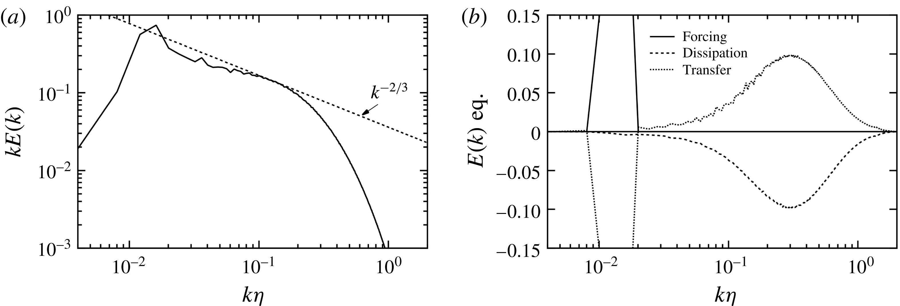
Figure 1(a) shows the profile of the premultiplied energy spectrum
 $kE(k)$
as a function of
 $k\unicode[STIX]{x1D702}$
. The Kolmogorov length scale
 $\unicode[STIX]{x1D702}(=\unicode[STIX]{x1D708}^{3/4}\unicode[STIX]{x1D700}^{-1/4})$
is
 $4.02\times 10^{-3}$
. A line of
 $kE(k)\propto k^{-2/3}$
for the inertial range is also plotted. The profile of
 $kE(k)$
exhibits its peak at
 $k\unicode[STIX]{x1D702}=0.016$
(
 $k=4$
) because of the external forcing. The inertial range is not clearly observed in the profile because the Reynolds number is not very high; the profile can be contaminated by the so-called bottleneck effect (Donzis & Sreenivasan Reference Donzis and Sreenivasan2010). Here, we just define an approximate inertial range by comparing with the line of
 $k^{-2/3}$
. The approximate inertial range, where
 $kE(k)\propto k^{-2/3}$
, is located at
 $0.08<k\unicode[STIX]{x1D702}<0.16$
. At
 $k\unicode[STIX]{x1D702}>0.16$
, the energy spectrum decays rapidly owing to the viscous effect.
Energy transport in the wavenumber space: (a) premultiplied energy spectrum
 $kE(k)$
as a function of
 $k\unicode[STIX]{x1D702}$
and (b) terms in the transport equation given by (3.1) as functions of
 $k\unicode[STIX]{x1D702}$
.

The transport equation for
 $E(k)$
given by (2.6) is rewritten as
 $$\begin{eqnarray}\frac{\unicode[STIX]{x2202}}{\unicode[STIX]{x2202}t}E(k)=-\unicode[STIX]{x1D700}(k)+T(k)+F(k).\end{eqnarray}$$
The forcing term, which is defined as
 $$\begin{eqnarray}F(k)=4\unicode[STIX]{x03C0}k^{2}\langle f_{i}^{\prime }(\boldsymbol{k})u_{i}^{\prime }(-\boldsymbol{k})\rangle ,\end{eqnarray}$$
is added, where
 $f_{i}^{\prime }(\boldsymbol{k})$
is the Fourier transform of external forcing
 $f_{i}^{\prime }(\boldsymbol{x})$
in the Navier–Stokes equation. Figure 1(b) shows the profiles of terms in the transport equation given by (3.1) as functions of
 $k\unicode[STIX]{x1D702}$
; each term is multiplied by
 $k$
, as in the case of figure 1(a). At
 $0.01\leqslant k\unicode[STIX]{x1D702}\leqslant 0.018$
(
 $2.5\leqslant k\leqslant 4.5$
), the forcing term
 $F(k)$
shows large positive values and the transfer term
 $T(k)$
shows large negative values. At
 $k\unicode[STIX]{x1D702}>0.018$
(
 $k>0.45$
),
 $T(k)$
shows positive values and is balanced by the negative dissipation term
 $-\unicode[STIX]{x1D700}(k)$
. The profile of
 $T(k)$
represents the energy cascade from low to high wavenumbers. These results indicate the well-known behaviour of homogeneous isotropic turbulence.
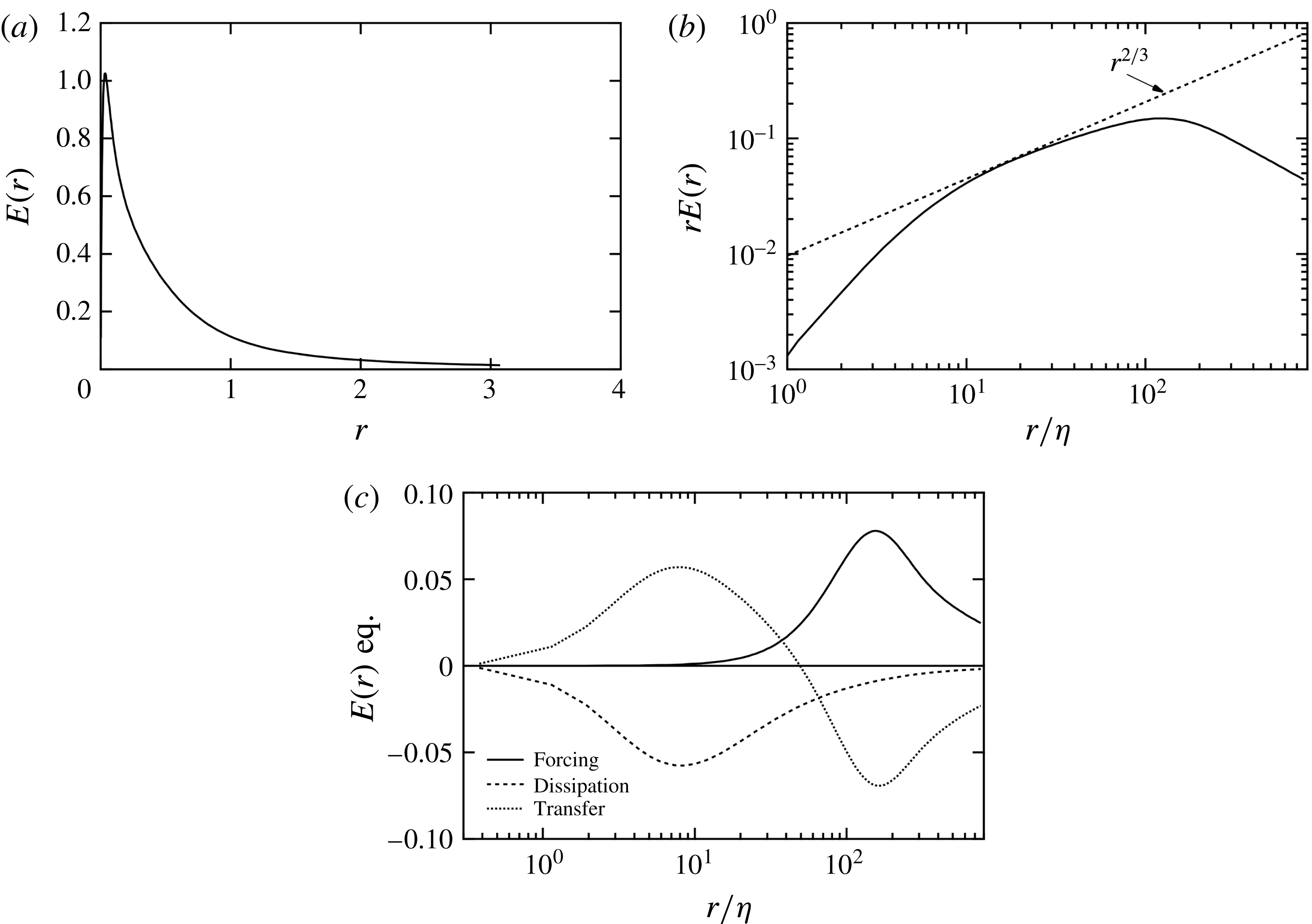
Energy transport in the scale space: (a) new energy density
 $E(r)$
as a function of
 $r$
, (b) premultiplied energy density
 $rE(r)$
as a function of
 $r/\unicode[STIX]{x1D702}$
in the log scale and (c) terms in the transport equation given by (3.3) as functions of
 $r/\unicode[STIX]{x1D702}$
.

Next, we examine the newly proposed energy density in the scale space and its transport equation. Figure 2(a) shows the profile of the energy density
 $E(r)$
given by (2.28) as a function of
 $r$
. The profile of
 $E(r)$
at large (small) scales in figure 2(a) corresponds to the profile of
 $E(k)$
at low (high) wavenumbers in figure 1(a). The energy density
 $E(r)$
exhibits its peak at
 $r=0.033$
(
 $r/\unicode[STIX]{x1D702}=8.3$
), and then decreases monotonically as
 $r$
increases. It should be noted that the location of the peak of
 $E(r)$
in the scale space corresponds to the dissipation range rather than the energy-containing range because the inertial range profile is
 $E(r)\propto r^{-1/3}$
, which decreases as
 $r$
increases (Hamba Reference Hamba2015). In order to see the small-scale part of
 $E(r)$
in more detail, and for comparison with
 $kE(k)$
in figure 1(a), we plot the premultiplied energy density
 $rE(r)$
as a function of
 $r/\unicode[STIX]{x1D702}$
on a log scale in figure 2(b). A line of
 $rE(r)\propto r^{2/3}$
for the inertial range is also plotted; the value increases as
 $r$
increases. The profile of
 $rE(r)$
exhibits its peak at
 $r/\unicode[STIX]{x1D702}=130$
(
 $r=0.5$
), which corresponds to the energy-containing range. The profile of the peak is not as sharp as that of
 $kE(k)$
in figure 1(a) because the energy density
 $E(r)$
is not determined by
 $\hat{Q}_{ii}(k)$
at a single wavenumber, but by the integral given by (2.28). The approximate inertial range of
 $rE(r)$
is located at
 $13<r/\unicode[STIX]{x1D702}<25$
(
 $0.05<r<0.1$
); it is narrow because the Reynolds number is not very high. As
 $r$
decreases, the profile at
 $r/\unicode[STIX]{x1D702}<13$
(
 $r<0.05$
) decreases rapidly compared to the line of
 $rE(r)\propto r^{2/3}$
; the profile represents the dissipation range. Therefore, the behaviour of the energy density
 $rE(r)$
shown in figure 2(b) is very similar to that of the energy spectrum
 $kE(k)$
shown in figure 1(a). It should be noted that rather than the energy density
 $E(r)$
itself, which is the energy per unit interval in
 $r$
, the premultiplied one
 $rE(r)$
, which corresponds to the energy per unit octave, is more convenient in examining the energy distribution in the scale space.
For homogeneous isotropic turbulence, the transport equation for
 $E(r)$
given by (2.39) can be rewritten as
 $$\begin{eqnarray}\frac{\unicode[STIX]{x2202}}{\unicode[STIX]{x2202}t}E(r)=-\unicode[STIX]{x1D700}(r)+T(r)+F(r).\end{eqnarray}$$
The production and diffusion terms disappear whereas the forcing term, which is defined as
 $$\begin{eqnarray}F(r)=-\frac{1}{2}\int _{-\infty }^{\infty }\text{d}\unicode[STIX]{x1D709}G_{D}(\unicode[STIX]{x1D709},r)\langle f_{i}^{\prime }(\boldsymbol{x})u_{i}^{\prime }(\boldsymbol{x}+\unicode[STIX]{x1D743})+f_{i}^{\prime }(\boldsymbol{x}+\unicode[STIX]{x1D743})u_{i}^{\prime }(\boldsymbol{x})\rangle ,\end{eqnarray}$$
is added. Figure 2(c) shows the profiles of terms in the transport equation given by (3.3) as functions of
 $r/\unicode[STIX]{x1D702}$
; each term is multiplied by
 $r$
. At large scales around
 $r/\unicode[STIX]{x1D702}=150$
(
 $r=0.6$
), the forcing term
 $F(r)$
shows positive values. This scale approximately corresponds to the location of the peak of
 $rE(r)$
shown in figure 2(b). Compared to
 $F(k)$
in figure 1(b), the profile of
 $F(r)$
is not sharp for the same reason as mentioned above for the profile of
 $rE(r)$
; although the forcing is limited at
 $2.5\leqslant k\leqslant 4.5$
in the wavenumber space, it shows a broad profile in the scale space because of the integral given by (2.28). The transfer term
 $T(r)$
shows negative values at large scales and positive values at small scales, where it is balanced by the negative dissipation term
 $-\unicode[STIX]{x1D700}(r)$
; the profile of
 $T(r)$
represents the energy cascade from large to small scales. Therefore, the behaviour of the transport equation for
 $E(r)$
is very similar to that of the transport equation for
 $E(k)$
shown in figure 1(b). These results indicate that the energy density
 $E(r)$
proposed in this work successfully describes the dynamics of homogeneous isotropic turbulence, as with the energy spectrum
 $E(k)$
.
4 Energy transport in turbulent channel flow
To determine whether the newly proposed energy density can be used to properly describe the energy transfer in the scale space in inhomogeneous turbulence, we examine DNS data of a turbulent channel flow. The simulation was carried out as follows. The size of the computational domain is
 $L_{x}\times L_{y}\times L_{z}=2\unicode[STIX]{x03C0}\times 2\times \unicode[STIX]{x03C0}$
, where
 $x$
,
 $y$
and
 $z$
denote the streamwise, wall-normal and spanwise directions, respectively. The number of grid points is
 $N_{x}\times N_{y}\times N_{z}=1024\times 192\times 1024$
. The Reynolds number based on the friction velocity
 $u_{\unicode[STIX]{x1D70F}}$
and the channel half-width
 $L_{y}/2$
is set to
 $Re_{\unicode[STIX]{x1D70F}}=590$
. The largest value of the micro-scale Reynolds number
 $R_{\unicode[STIX]{x1D706}}$
is 61.7 at
 $y^{+}=259$
; it is not as large as the value of
 $R_{\unicode[STIX]{x1D706}}=161$
for the homogeneous isotropic turbulence examined in § 3. Hereafter, physical quantities are non-dimensionalized by
 $u_{\unicode[STIX]{x1D70F}}$
and
 $L_{y}/2$
. The periodic boundary conditions are used in the streamwise and spanwise directions, and the no-slip conditions are imposed at the wall at
 $y=0$
and
 $y=2$
. We use the second-order finite-difference scheme in space and the Adams–Bashforth method for time marching. Because the scheme is not a high-order one, the number of grid points was increased so that accurate results can be obtained. Statistical quantities such as the velocity correlation are obtained by averaging over the
 $x$
–
 $z$
plane and over a time period of 30 normalized by
 $(L_{y}/2)/u_{\unicode[STIX]{x1D70F}}$
.
Because the channel flow is homogeneous in the
 $x$
and
 $z$
directions and inhomogeneous in the
 $y$
direction, statistical quantities depend on
 $y$
only. The energy density defined as (2.33) can be written as
 $$\begin{eqnarray}E(y,r_{j})=\frac{1}{2}\int _{-\infty }^{\infty }\text{d}\unicode[STIX]{x1D709}_{j}G_{D}(\unicode[STIX]{x1D709}_{j},r_{j})Q_{ii}(y,\unicode[STIX]{x1D709}_{j}),\end{eqnarray}$$
where summation is not taken for
 $j$
. The turbulent kinetic energy can be decomposed into the energy density in one-dimensional scale space as
 $$\begin{eqnarray}K(y)=\int _{0}^{\infty }\text{d}r_{j}E(y,r_{j}).\end{eqnarray}$$
This decomposition depends on the direction of the scale space; that is, the direction of length scale
 $r_{j}$
for inhomogeneous turbulence. In this work, for each statistical quantity, we investigate three cases: the streamwise scale space
 $r_{x}$
, spanwise scale space
 $r_{z}$
, and wall-normal scale space
 $r_{y}$
.
First, we compare the energy density given by (4.1) with the previous one proposed by Hamba (Reference Hamba2015) as follows:
 $$\begin{eqnarray}E(y,r_{j})=-\frac{\unicode[STIX]{x2202}}{\unicode[STIX]{x2202}r_{j}}\frac{1}{2}Q_{ii}(y,r_{j}),\end{eqnarray}$$
in the three cases. In the previous expression, the length scale
 $r_{j}$
in the velocity correlation
 $Q_{ii}(y,r_{j})$
is the separation itself. We examine statistical quantities obtained at
 $y=0.2$
(
 $y^{+}=119$
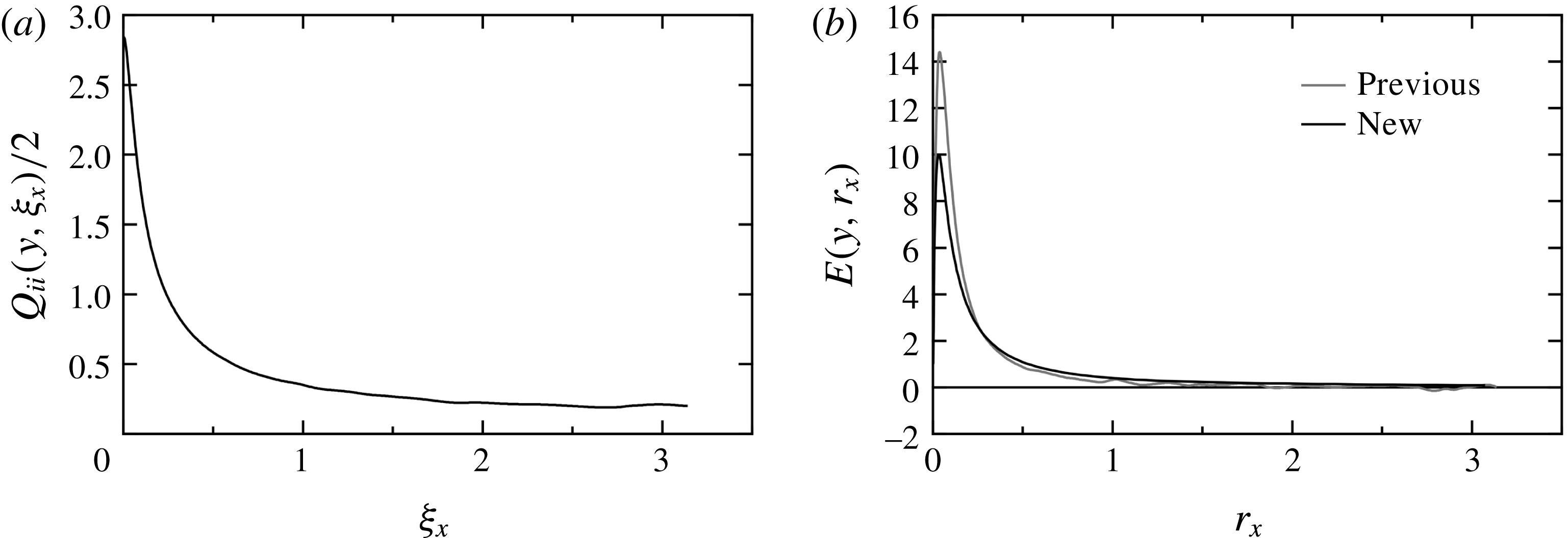
) in the log layer of the channel flow. In figure 3(a), we plot the profile of the velocity correlation
 $Q_{ii}(y,\unicode[STIX]{x1D709}_{x})/2$
as a function of
 $\unicode[STIX]{x1D709}_{x}$
at
 $y^{+}=119$
to examine the case of the streamwise scale space. The profile decreases monotonically as
 $\unicode[STIX]{x1D709}_{x}$
increases. This monotonic decrease is desirable for the previous expression given by (4.3) because it is expected to yield positive values of the energy density in the whole region. Figure 3(b) shows the profiles of the previous and new energy densities
 $E(y,r_{x})$
as functions of
 $r_{x}$
at
 $y^{+}=119$
. Both profiles are similar to that for homogeneous isotropic turbulence shown in figure 2(a). The peak of the new energy density is lower than that of the previous one because the integral in the new expression smooths the profile to some extent. As
 $r_{x}$
increases, both profiles decrease to very small positive values, with the exception that the previous energy density shows very small negative values around
 $r_{x}=3$
because of a slight oscillation of
 $Q_{ii}(y,\unicode[STIX]{x1D709}_{x})/2$
. Therefore, the overall profiles of the previous and new energy densities are similar to each other in the streamwise scale space.
Energy density in the streamwise scale space at
 $y^{+}=119$
: (a) two-point velocity correlation
 $Q_{ii}(y,\unicode[STIX]{x1D709}_{x})/2$
as a function of
 $\unicode[STIX]{x1D709}_{x}$
and (b) previous and new expressions for energy density
 $E(y,r_{x})$
as functions of
 $r_{x}$
.

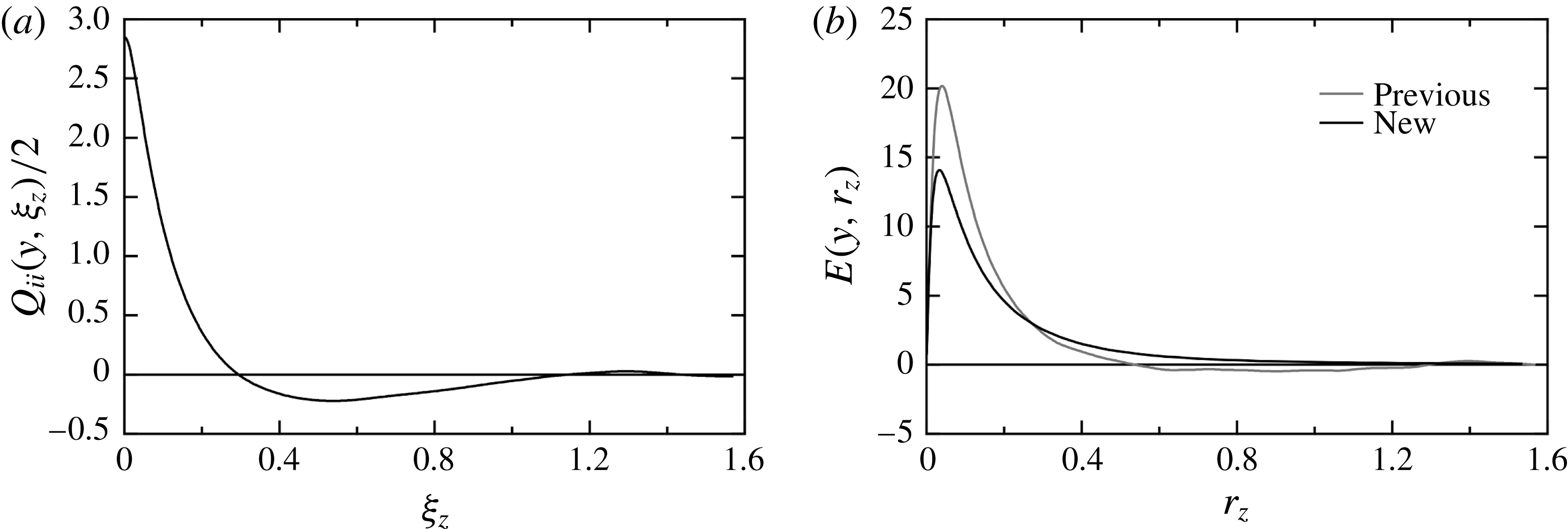
In figure 4(a), we plot the profile of the velocity correlation
 $Q_{ii}(y,\unicode[STIX]{x1D709}_{z})/2$
as a function of
 $\unicode[STIX]{x1D709}_{z}$
at
 $y^{+}=119$
to examine the case of the spanwise scale space. In contrast to the streamwise correlation, the spanwise correlation clearly exhibits negative values at
 $0.3<\unicode[STIX]{x1D709}_{z}<1.1$
. This negative correlation is closely related to the streaky structure of the velocity fluctuation
 $u_{x}^{\prime }$
. Figure 4(b) shows the profiles of the previous and new energy densities
 $E(y,r_{z})$
as functions of
 $r_{z}$
at
 $y^{+}=119$
. In this case, the previous energy density exhibits negative values at
 $0.54<r_{z}<1.3$
. This is because the velocity correlation
 $Q_{ii}(y,\unicode[STIX]{x1D709}_{z})/2$
increases as
 $\unicode[STIX]{x1D709}_{z}$
increases in this region in figure 4(a). In contrast, the profile of the new energy density shows positive values in the whole region, as expected. Because the turbulent field is homogeneous in the spanwise direction,
 $E(y,r_{z})\geqslant 0$
is satisfied.
Energy density in the spanwise scale space at
 $y^{+}=119$
: (a) two-point velocity correlation
 $Q_{ii}(y,\unicode[STIX]{x1D709}_{z})/2$
as a function of
 $\unicode[STIX]{x1D709}_{z}$
and (b) previous and new expressions for energy density
 $E(y,r_{z})$
as functions of
 $r_{z}$
.

In figure 5(a), we plot the profile of the velocity correlation
 $Q_{ii}(y,\unicode[STIX]{x1D709}_{y})/2$
as a function of
 $|\unicode[STIX]{x1D709}_{y}|$
at
 $y^{+}=119$
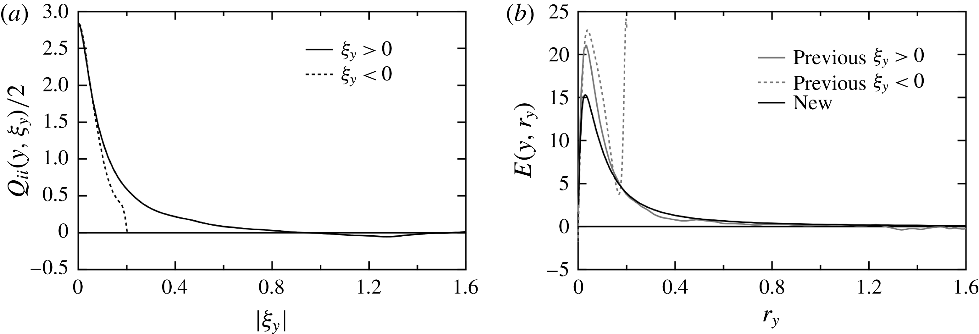
to examine the case of the wall-normal scale space. Because the turbulent field is inhomogeneous in the wall-normal direction, the profiles of the correlation in the positive and negative
 $y$
directions are different; profiles for both
 $\unicode[STIX]{x1D709}_{y}>0$
and
 $\unicode[STIX]{x1D709}_{y}<0$
are plotted. The two profiles are similar to each other at
 $\left|\unicode[STIX]{x1D709}_{y}\right|<0.1$
, while the profile for
 $\unicode[STIX]{x1D709}_{y}<0$
rapidly decreases to zero at
 $\left|\unicode[STIX]{x1D709}_{y}\right|=0.2$
because the value of
 $\unicode[STIX]{x1D709}_{y}=-0.2$
corresponds to the location of the bottom wall at
 $y=0$
. Figure 5(b) shows the profiles of the previous and new energy densities
 $E(y,r_{y})$
as functions of
 $r_{y}$
at
 $y^{+}=119$
. Because the velocity correlation
 $Q_{ii}(y,\unicode[STIX]{x1D709}_{y})/2$
directly affects
 $E(y,r_{y})$
with
 $r_{y}=\unicode[STIX]{x1D709}_{y}$
for the previous expression, the energy density for
 $\unicode[STIX]{x1D709}_{y}<0$
is limited to the scales at
 $0\leqslant r_{y}\leqslant 0.2$
; its profile changes rapidly as
 $r_{y}$
approaches 0.2 because of the wall effect. In contrast, for the new expression given by (4.1), the length scale
 $r_{y}$
is not the separation itself but the filter width appearing in
 $G_{D}(\unicode[STIX]{x1D709}_{y},r_{y})$
; the length scale
 $r_{y}$
can be longer than the distance to the wall. The profile of the new energy density
 $E(y,r_{y})$
is similar to those in the other two cases shown in figures 3(b) and 4(b). Although non-negative values are not guaranteed because of the inhomogeneity,
 $E(y,r_{y})$
shows positive values in the whole region in figure 5(b). Therefore, the new expression for the energy density is better than the previous expression. Hereafter, we investigate the statistics for the new energy density.
Energy density in the wall-normal scale space at
 $y^{+}=119$
: (a) two-point velocity correlations
 $Q_{ii}(y,\unicode[STIX]{x1D709}_{y})/2$
as functions of
 $|\unicode[STIX]{x1D709}_{y}|$
and (b) previous and new expressions for energy density
 $E(y,r_{y})$
as functions of
 $r_{y}$
.

So far, we have examined the profiles of
 $E(y,r_{j})$
as functions of
 $r_{j}$
. Because the energy density depends not only on
 $r_{j}$
but also on
 $y$
, we now examine two-dimensional plots of the new energy density
 $E(y,r_{j})$
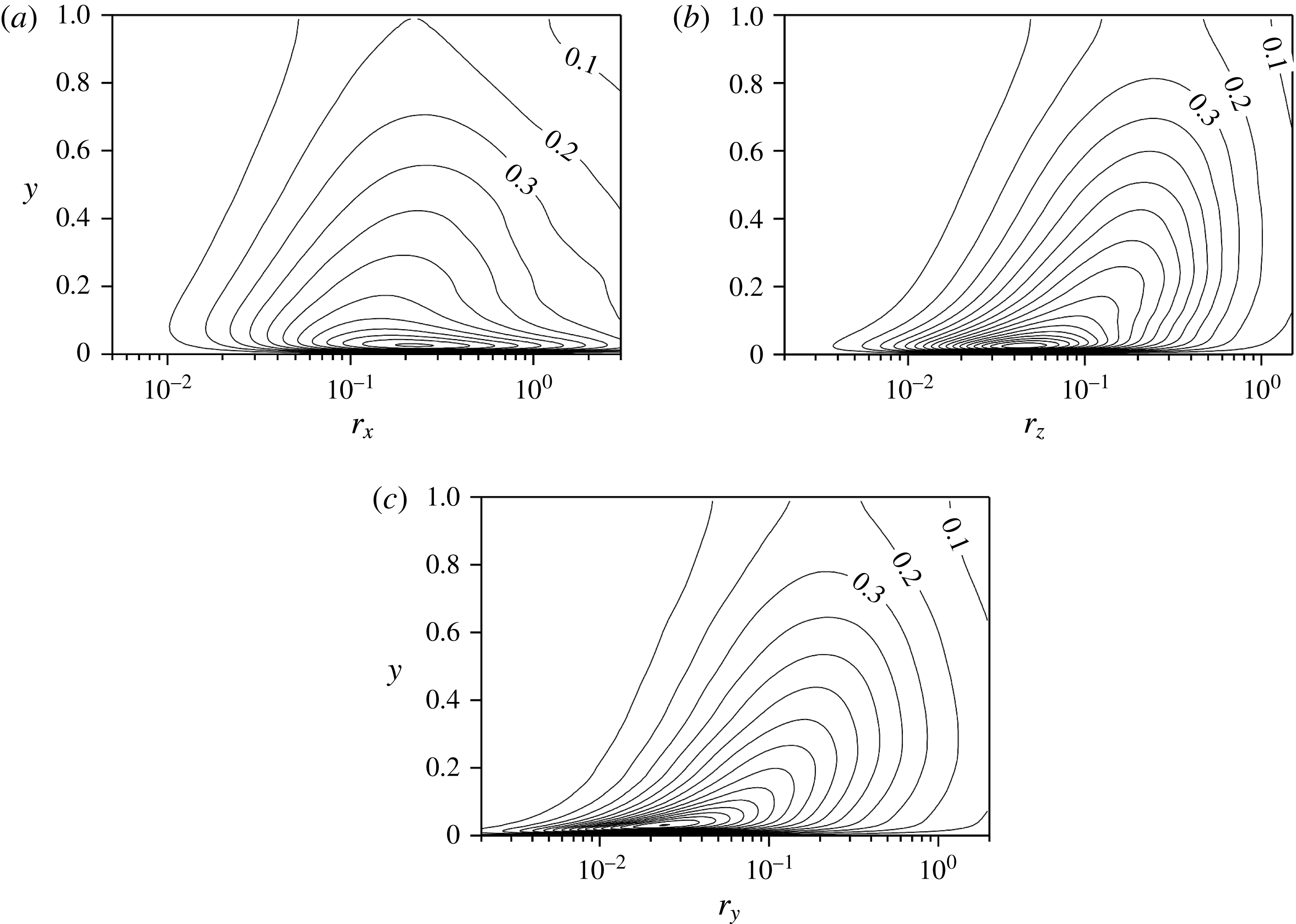
. Figure 6(a) shows the contours of the premultiplied energy density
 $r_{x}E(y,r_{x})$
given by (4.1) in the
 $r_{x}$
–
 $y$
plane. The bottom wall of the channel corresponds to
 $y=0$
and the channel centre to
 $y=1$
. The peak of
 $r_{x}E(y,r_{x})$
is located at
 $r_{x}=0.23$
and
 $y=0.025$
(
 $y^{+}=15$
). The location of the peak of
 $r_{x}E(y,r_{x})$
with respect to
 $r_{x}$
for a fixed value of
 $y$
represents the streamwise length scale of the energy-containing range at each
 $y$
location, as shown in figure 2(b) for homogeneous isotropic turbulence. The peak location does not change significantly as
 $y$
increases; the streamwise length scale of the turbulent field near the wall is as long as that apart from the wall. Figure 6(b) shows the contours of the premultiplied energy density
 $r_{z}E(y,r_{z})$
given by (4.1) in the
 $r_{z}$
–
 $y$
plane. The peak of
 $r_{z}E(y,r_{z})$
is located at
 $r_{z}=0.046$
and
 $y=0.025$
(
 $y^{+}=15$
). In contrast to the case of
 $r_{x}E(y,r_{x})$
in figure 6(a), the peak location with respect to
 $r_{z}$
or the spanwise length scale is the smallest near the wall, and it increases as
 $y$
increases. The difference in the peak location near the wall between the streamwise and spanwise scale spaces suggests the strong anisotropy of the length scale. Figure 6(c) shows the contours of the premultiplied energy density
 $r_{y}E(y,r_{y})$
given by (4.1) in the
 $r_{y}$
–
 $y$
plane. The peak of
 $r_{y}E(y,r_{y})$
is located at
 $r_{y}=0.025$
and
 $y=0.032$
(
 $y^{+}=19$
). As mentioned above,
 $E(y,r_{y})$
is not guaranteed to be non-negative. In fact, it takes small negative values in a narrow region near the wall at
 $r_{y}<0.0147$
and
 $y^{+}<1.9$
. Nevertheless, it shows positive values in almost all regions in figure 6(c). The profile of
 $r_{y}E(y,r_{y})$
is similar to that of
 $r_{z}E(y,r_{z})$
, as shown in figure 6(b); this suggests that the new expression for the energy density is adequately applied to the scale space of the inhomogeneous direction. The reason why negative values are observed near the wall is not clear at present. The behaviour may change if a sharper filter function is adopted. Considering the discussion on (2.38), we expect that the energy density defined using double integrals similar to (2.36) would always give non-negative values even for inhomogeneous turbulence. But, such an energy density is too complex to apply to actual turbulence. As future work, the criterion for a non-negative value of the present energy density should be studied.
Contour plots of premultiplied energy density: (a)
 $r_{x}E(y,r_{x})$
in the
 $r_{x}$
–
 $y$
plane, (b)
 $r_{z}E(y,r_{z})$
in the
 $r_{z}$
–
 $y$
plane and (c)
 $r_{y}E(y,r_{y})$
in the
 $r_{y}$
–
 $y$
plane.

Next, we analyse the transport equation for the energy density given by (2.39). Because the equation has many terms, it is very complex to examine all terms in the
 $r_{j}$
–
 $y$
plane. Here, we evaluate them as functions of length scale
 $r_{j}/\unicode[STIX]{x1D702}$
at
 $y=0.2$
(
 $y^{+}=119$
). The Kolmogorov length scale
 $\unicode[STIX]{x1D702}$
is
 $4.62\times 10^{-3}$
at
 $y^{+}=119$
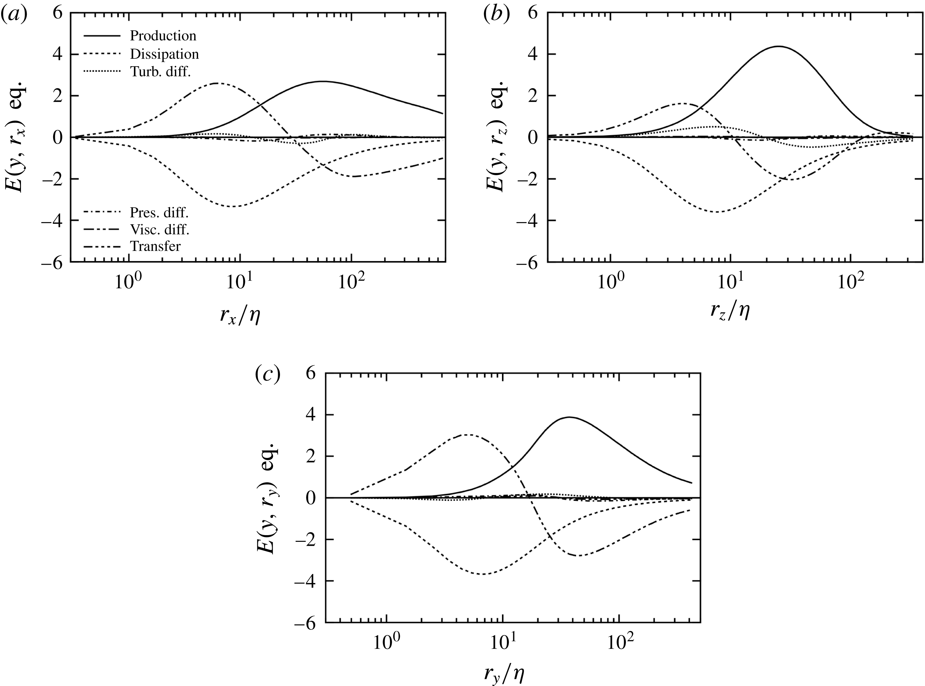
. Figure 7(a) shows the profiles of terms in the transport equation for
 $E(y,r_{x})$
given by (2.39) as functions of
 $r_{x}/\unicode[STIX]{x1D702}$
at
 $y^{+}=119$
; each term is multiplied by
 $r_{x}$
. The production, dissipation and transfer terms are dominant in this budget. The production term is positive at large scales around
 $r_{x}/\unicode[STIX]{x1D702}=56$
(
 $r_{x}=0.26$
); the location of the peak of the production term corresponds to that of
 $r_{x}E(y,r_{x})$
, as shown in figure 6(a). The transfer term shows negative values at large scales and positive values at small scales, where it is nearly balanced by the negative dissipation term; the profile of the transfer term represents the energy cascade from large to small scales. This behaviour is very similar to that of the transport equation for the homogeneous isotropic turbulence shown in figure 2(c) when the production term is considered to play the same role as the forcing term. Figure 7(b) shows the profiles of terms in the transport equation for
 $E(y,r_{z})$
given by (2.39) as functions of
 $r_{z}/\unicode[STIX]{x1D702}$
at
 $y^{+}=119$
. The overall behaviour is similar to that of
 $E(y,r_{x})$
, as shown in figure 7(a); the energy produced at large scales is transferred to small scales, and is dissipated there because of the viscous effect. We can see small positive values of the transfer term at very large scales at
 $r_{z}/\unicode[STIX]{x1D702}>130$
(
 $r_{z}>0.6$
). The positive values suggest the inverse energy cascade from large to very large scales; a small part of the produced energy is transferred to eddies of very large size. Such an inverse cascade would be caused by turbulent structures close to two-dimensional. The inverse cascade is not seen in the streamwise scale space in figure 7(a). Figure 7(c) shows the profiles of terms in the transport equation for
 $E(y,r_{y})$
given by (2.39) as functions of
 $r_{y}/\unicode[STIX]{x1D702}$
at
 $y^{+}=119$
. The behaviour is very similar to that of
 $E(y,r_{x})$
shown in figure 7(a). The typical energy cascade from large to small scales is clearly observed, even in the scale space of the inhomogeneous wall-normal direction. Not only the
 $r_{j}$
dependence but also the energy
 $\langle u_{\unicode[STIX]{x1D6FC}}^{\prime 2}\rangle$
itself (summation is not taken for
 $\unicode[STIX]{x1D6FC}$
) is clearly anisotropic in turbulent channel flow. The transport equation for the streamwise, wall-normal and spanwise parts of the energy density can be derived in a similar form to (2.39). As future work, the transport of the three energies in the scale space will be analysed.
Terms in the transport equation given by (2.39) at
 $y^{+}=119$
(a) for
 $E(y,r_{x})$
as functions of
 $r_{x}/\unicode[STIX]{x1D702}$
, (b) for
 $E(y,r_{z})$
as functions of
 $r_{z}/\unicode[STIX]{x1D702}$
and (c) for
 $E(y,r_{y})$
as functions of
 $r_{y}/\unicode[STIX]{x1D702}$
.

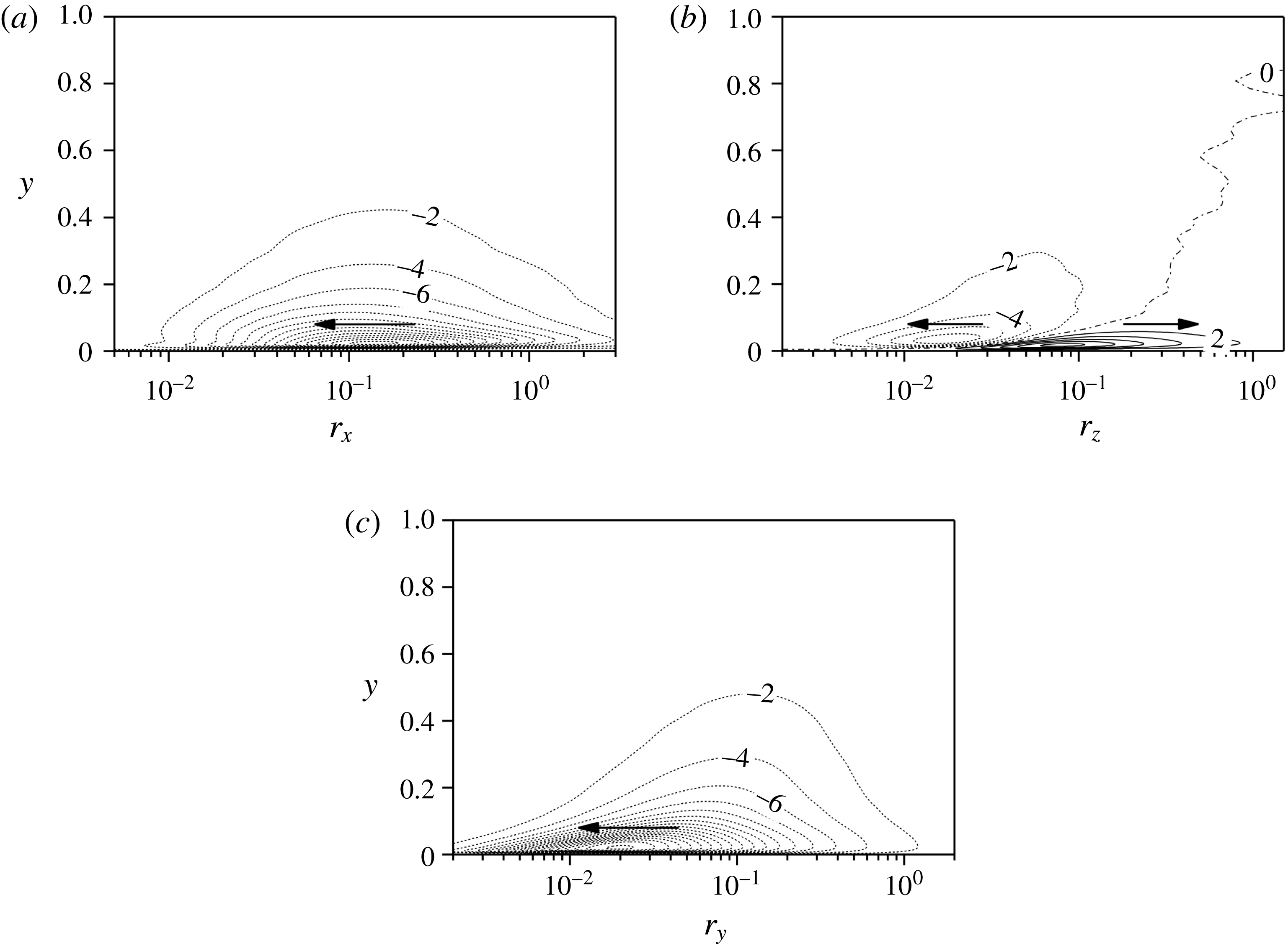
Contour plots of energy flux in the scale space: (a)
 $\unicode[STIX]{x1D6F1}(y,r_{x})$
in the
 $r_{x}$
–
 $y$
plane, (b)
 $\unicode[STIX]{x1D6F1}(y,r_{z})$
in the
 $r_{z}$
–
 $y$
plane and (c)
 $\unicode[STIX]{x1D6F1}(y,r_{y})$
in the
 $r_{y}$
–
 $y$
plane. Arrows denote the direction of the energy cascade.

Here, we focus on the energy flux in the scale space. The transfer term given by (2.45) is rewritten as
 $$\begin{eqnarray}T(y,r_{k})=-\frac{\unicode[STIX]{x2202}}{\unicode[STIX]{x2202}r_{k}}\unicode[STIX]{x1D6F1}(y,r_{k}),\end{eqnarray}$$
where the energy flux in the scale space is given by
 $$\begin{eqnarray}\displaystyle \unicode[STIX]{x1D6F1}(y,r_{k}) & = & \displaystyle -\frac{1}{2}\int _{-\infty }^{\infty }\text{d}\unicode[STIX]{x1D709}_{k}G(\unicode[STIX]{x1D709}_{k},r_{k})\frac{\unicode[STIX]{x2202}}{\unicode[STIX]{x2202}\unicode[STIX]{x1D709}_{j}}\langle (u_{j}^{\prime }(\boldsymbol{x}+\unicode[STIX]{x1D743})-u_{j}^{\prime }(\boldsymbol{x}))u_{i}^{\prime }(\boldsymbol{x})u_{i}^{\prime }(\boldsymbol{x}+\unicode[STIX]{x1D743})\rangle \nonumber\\ \displaystyle & & \displaystyle -\frac{1}{2}\int _{-\infty }^{\infty }\text{d}\unicode[STIX]{x1D709}_{k}G(\unicode[STIX]{x1D709}_{k},r_{k})\frac{\unicode[STIX]{x2202}}{\unicode[STIX]{x2202}\unicode[STIX]{x1D709}_{j}}[(U_{j}(\boldsymbol{x}+\unicode[STIX]{x1D743})-U_{j}(\boldsymbol{x}))\langle u_{i}^{\prime }(\boldsymbol{x})u_{i}^{\prime }(\boldsymbol{x}+\unicode[STIX]{x1D743})\rangle ],\end{eqnarray}$$
and
 $\unicode[STIX]{x1D743}=\unicode[STIX]{x1D709}_{k}\boldsymbol{e}_{k}$
(summation is not taken for
 $k$
). The second line of (4.5) disappears when
 $\unicode[STIX]{x1D709}_{k}$
is directed in the homogeneous direction because
 $U_{j}(\boldsymbol{x}+\unicode[STIX]{x1D743})=U_{j}(\boldsymbol{x})$
. Figure 8 shows the contours of the energy flux
 $\unicode[STIX]{x1D6F1}(y,r_{k})$
given by (4.5) in the
 $r_{k}$
–
 $y$
plane in the three cases:
 $r_{k}=r_{x}$
,
 $r_{z}$
and
 $r_{y}$
. Contours of positive (negative) values are plotted in solid (dashed) lines. Arrows plotted in the figures denote the direction of the energy cascade. In figure 8(a,c), all contours are negative values, indicating the energy cascade from large to small scales. In contrast, in figure 8(b), contours of both positive and negative values are seen; the forward cascade is observed at relatively small scales, whereas the inverse cascade is clearly seen at large scales near the wall. Even apart from the wall, the inverse cascade is observed at very large scales, as indicated by the transfer term in the
 $E(y,r_{z})$
equation in figure 7(b). In figure 8(b), the zero flux boundary is approximately given by the line
 $y=r_{z}$
, which suggests that turbulent structures associated with the inverse cascade are limited at larger scales in the
 $z$
-direction and tend to be slightly two-dimensional.
Cimarelli et al. (Reference Cimarelli, De Angelis and Casciola2013) investigated the energy flux in the physical and scale spaces of turbulent channel flows using the transport equation for the structure function. They examined paths of the energy flux in the
 $r_{x}$
–
 $Y_{c}$
and
 $r_{z}$
–
 $Y_{c}$
planes, where
 $Y_{c}$
is the wall-normal coordinate of the midpoint of the velocity increment. They also showed the forward and inverse energy cascades corresponding to figure 8(a,b), respectively. Thus, it is expected that the inverse cascade in the spanwise scale space is present. Cimarelli et al. (Reference Cimarelli, De Angelis, Jiménez and Casciola2016) examined the energy flux in the
 $(r_{y},r_{z},Y_{c})$
plane in detail, and showed the inverse cascade in the wall-normal scale space. This behaviour is different from our result in that only the forward cascade is observed in figure 8(c). The difference in the cascade may be attributed to the difference between the structure function and the present energy density; as future work, the behaviour of the energy flux in the wall-normal scale space will be studied.
Finally, we examine the energy flux in the wall-normal direction in the physical space. We evaluate the turbulent diffusion term
 $D_{T}$
because it is dominant among the three diffusion terms. The turbulent diffusion term given by (2.42) is rewritten as
 $$\begin{eqnarray}D_{T}(y,r_{k})=-\frac{\unicode[STIX]{x2202}}{\unicode[STIX]{x2202}y}\unicode[STIX]{x1D6F7}_{Ty}(y,r_{k}),\end{eqnarray}$$
where the energy flux in the wall-normal direction is given by
 $$\begin{eqnarray}\unicode[STIX]{x1D6F7}_{Ty}(y,r_{k})=\frac{1}{2}\int _{-\infty }^{\infty }\text{d}\unicode[STIX]{x1D709}_{k}G_{D}(\unicode[STIX]{x1D709}_{k},r_{k})\langle u_{y}^{\prime }(\boldsymbol{x})u_{i}^{\prime }(\boldsymbol{x})u_{i}^{\prime }(\boldsymbol{x}+\unicode[STIX]{x1D743})\rangle .\end{eqnarray}$$
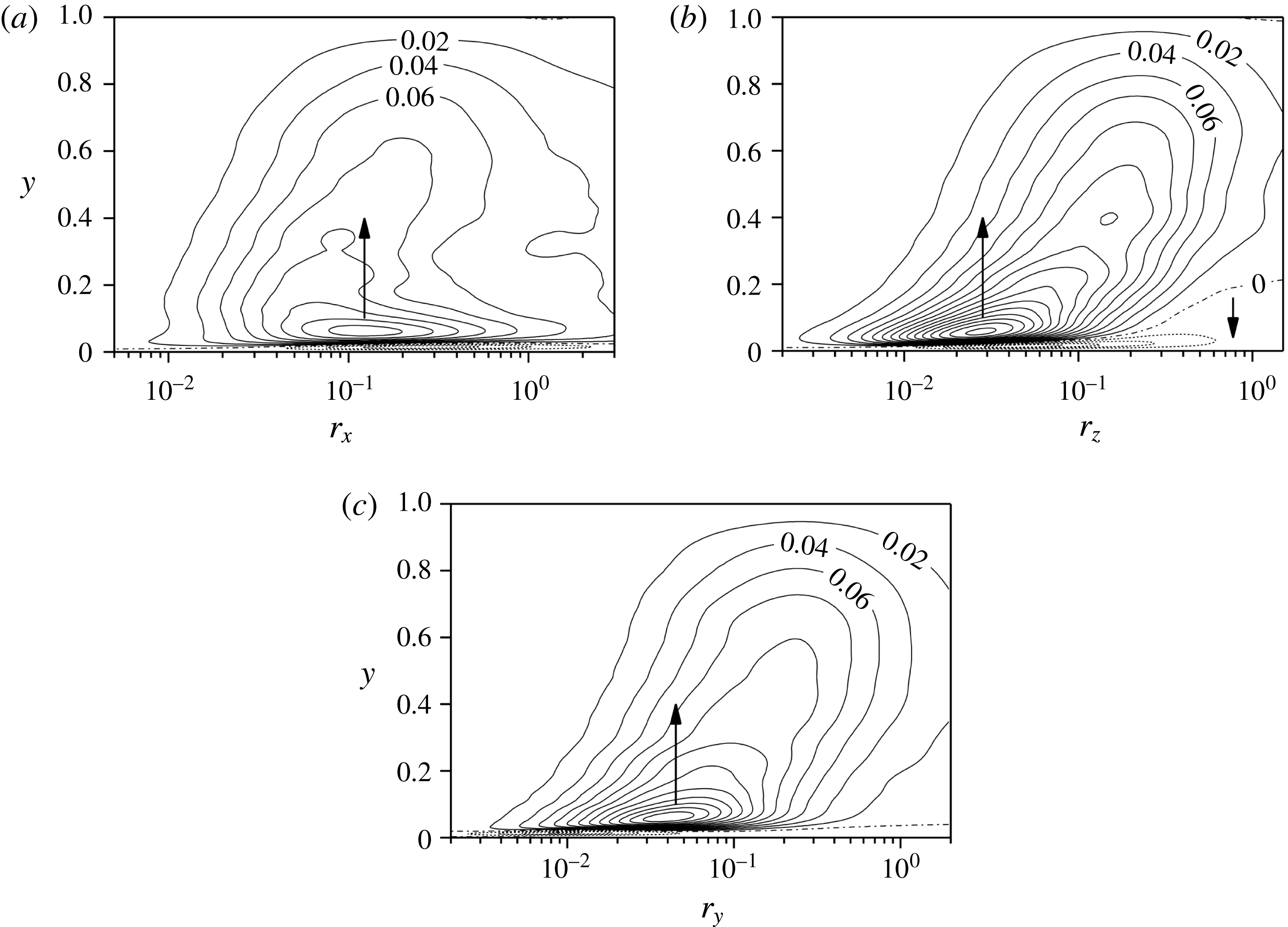
Figure 9 shows the contours of the premultiplied energy flux
 $r_{k}\unicode[STIX]{x1D6F7}_{Ty}(y,r_{k})$
given by (4.7) in the
 $r_{k}$
–
 $y$
plane in the three cases:
 $r_{k}=r_{x}$
,
 $r_{z}$
and
 $r_{y}$
. Arrows plotted in the figures denote the direction of the energy flux; those very close to the bottom wall are omitted. In figure 9(a,c), the energy flux shows positive values in almost all regions, except for the near-wall region, where it is negative. This is because the energy density whose peak is located at
 $y^{+}=15$
is expected to drive an upward flux at
 $y^{+}>15$
and a downward flux at
 $y^{+}<15$
. The profiles of positive contours shown in figure 9(a,c) are similar to those of the energy density itself shown in figure 6(a,c), respectively. In figure 9(b), the overall profiles of contours are similar to those of figure 9(c). However, we can see that the contour of zero value plotted as the dash-dotted line is apart from the wall at large scales at
 $r_{z}>0.3$
. This contour suggests that a downward flux is present at large scales, even apart from the wall. Mizuno (Reference Mizuno2016) examined the spectral energy budget equation for a turbulent channel flow to reveal the scale dependence of the energy transport. He examined the cospectra of the wall-normal flux of energy as functions of the spanwise wavelength
 $\unicode[STIX]{x1D706}_{z}$
, and showed an upward flux at small scales and a downward flux at large scales. This behaviour is similar to the present result shown in figure 9(b).
Contour plots of premultiplied energy flux in the physical space: (a)
 $r_{x}\unicode[STIX]{x1D6F7}_{Ty}(y,r_{x})$
in the
 $r_{x}$
–
 $y$
plane, (b)
 $r_{z}\unicode[STIX]{x1D6F7}_{Ty}(y,r_{z})$
in the
 $r_{z}$
–
 $y$
plane and (c)
 $r_{y}\unicode[STIX]{x1D6F7}_{Ty}(y,r_{y})$
in the
 $r_{y}$
–
 $y$
plane. Arrows denote the direction of the energy flux.

5 Conclusions
A new expression for the energy density in the scale space was proposed by using the integral of the two-point velocity correlation with a filter function. The new energy density satisfies the properties in that it is non-negative in the scale space of the homogeneous direction and its integral equals the turbulent kinetic energy. It was also shown that the energy density is closely related to the turbulent kinetic energy of the filtered velocity. The transport equation for the energy density was derived for inhomogeneous turbulence. The equation involves the energy transfer terms not only in the physical space but also in the scale space.
DNS data obtained for homogeneous isotropic turbulence were first used to evaluate the energy density and its transport equation. The energy transfer term showed the energy cascade from large to small scales. The behaviour of the energy density in the scale space is similar to that of the energy spectrum in the wavenumber space. The results indicate that the new energy density successfully describes the dynamics of homogeneous isotropic turbulence as with the energy spectrum.
DNS data of a turbulent channel flow were then used to evaluate the energy density and its transport equation in inhomogeneous turbulence. The energy density depends on the direction of the scale space. For each statistical quantity, we investigated three cases: the streamwise, spanwise and wall-normal scale spaces. It was shown that the energy density is positive in the streamwise and spanwise scale spaces. It is also positive in almost all regions of the wall-normal scale space. The energy transfer was successfully examined in the scale space not only in the homogeneous direction but also in the inhomogeneous direction. The energy cascade from large to small scales was clearly observed in the three cases. Moreover, the inverse energy cascade from large to very large scales was observed in the spanwise scale space. The energy flux in the wall-normal direction in the physical space was also examined. In addition to the main upward flux, a downward flux was observed at very large scales in the spanwise scale space. The advantage of the energy density in the scale space compared with the energy spectrum is that we can examine the scale dependence of the turbulent fluctuations even in the scale space of the inhomogeneous direction. We believe that the analysis of the transport equation for the energy density in the scale space is helpful for obtaining a better understanding of inhomogeneous turbulence and for realizing improvements in turbulence models.
Acknowledgements
This work was supported by JSPS KAKENHI Grant number JP17K06143.