What drove the Great Depression of the 1930s? The discussion on the origins, depth, and duration of the Great Depression in the United States has lately been dominated by a new set of questions that are strongly related to real side factors. According to mainstream explanations, the Great Depression was a response to monetary contraction caused by bank failures and bad monetary policy. High real interest rates depressed consumption and investment, arguably strengthened by the transmitting mechanism of the gold standard.Footnote 1 In contrast, the real business cycle (RBC) view holds that technology (or productivity) shocks should be held responsible for the decline in output levels instead of demand shocks resulting from financial and monetary distress. Proponents of the RBC approach have pointed at the widely observed procyclical relationship between output levels and fluctuations in total factor productivity (TFP), measured as a detrended Solow residual in total GDP growth.Footnote 2 One of the key contributions to this line of research for the American Depression economy is the work of Harold Cole and Lee Ohanian. Using an RBC model they put forward the idea that short-run fluctuations or shifts in the production function put downward pressure on the economy during the 1930s. According to this view technological regression (or some efficiency related factor) in the U.S. economy resulted in a contraction of inputs causing the Great Depression.Footnote 3
The main contribution of our article is to show that the Solow TFP residual is an unfit measure on which to base such a conclusion, because it is a biased technology measure in the presence of market power or labor and capital hoarding.Footnote 4 In an analysis of the postwar U.S. economy, Susanto Basu, John Fernald, and Miles Kimball estimate production functions to take market power and hoarding into account. Using the resulting “purified” technology measure, they find no positive correlation between technology shocks and input utilization.Footnote 5 In this article, we are the first to apply their methodology to the interwar period and we find similar results, contradicting the predictions of RBC theory. Moreover, we establish that labor and capital hoarding rather than market power was the dominant reason for the decline in the Solow TFP residual after 1929.
The development of new, detailed manufacturing data is crucial to reaching these conclusions. Several studies on the procyclical behavior of productivity for the pre-1945 period rely on time series for the total economy or on output indices of selected branches within manufacturing.Footnote 6 The present study builds on data taken from the Biennial Census of Manufactures, which covers total U.S. manufacturing for the period 1919–1939, classified into 19 industrial branches. Our analysis is greatly helped by this underutilized data source as the census provides a comprehensive account of manufacturing; a consistent set of output and input measures; and measures of gross output rather than the more commonly used value added.
We find that Solow residual TFP is an imperfect technology measure because it assumes constant returns to scale, while our estimates show that U.S. manufacturing industries are characterized by short-run increasing returns to scale. Following Basu, Fernald, and Kimball, we use the estimates of returns to scale to calculate a “purified” measure of technology change that takes into account that production is characterized by increasing returns to scale.Footnote 7 We test the RBC hypothesis that inputs follow technology shocks procyclically and find that movements in technology have no significant effect on any input, which is consistent with the findings of Basu, Fernald, and Kimball for the U.S. postwar economy. This leads us to conclude that, in contrast to RBC theory, the Great Depression in the United States was not caused by negative technology shocks. This minimizes the scope for views that attribute the interwar productivity decrease to lower production efficiency.Footnote 8
We also examine the source of the increasing returns to scale. In our empirical framework, we distinguish between market power and hoarding of labor and capital as two possible (nonexclusive) causes. We use a gross output framework to find evidence of both capital and labor hoarding, which is much harder to find in the value added framework used by others.Footnote 9 Our production function estimates show that output responds more strongly to changes in intermediate inputs than what could be expected on the basis of the cost share of these inputs, while the output elasticities of labor and of capital are equal to their cost shares. This supports the hypothesis of labor and capital hoarding and contrasts with the market power hypothesis. The empirical proof is consistent with recent historical research on the procyclicality of Solow residual TFP for the total U.S. economy.Footnote 10
PRODUCTIVITY SHOCKS AND THE GREAT DEPRESSION
During the Great Contraction from 1929 to 1933, the U.S. economy exhibited an extremely poor record in output growth and factor utilization. Total nonfarm GDP declined by 34 percent and total hours worked by 31 percent. The decline in manufacturing was even more severe, with declines of 37 and 40 percent for output and working hours respectively.Footnote 11 During this period, movements in productivity were procyclical. A detrended time series of Solow residual TFP for the U.S. economy reveals a decline of circa 18 percent between 1929 and 1933. In a paper published in 1991, Ben Bernanke and Martin Parkinson have explained the procyclical relationship between movements in output and productivity by pointing at the effects of labor hoarding and “true” increasing returns.Footnote 12 In contrast with this view and in support of RBC theory, Cole and Ohanian have interpreted the fall in Solow residual TFP not as a result of increasing returns but as a major exogenous technology shock. In a range of papers, they have tried to show how this shock led to decreasing marginal returns to capital and labor, and hence to a decline in employment and in the use of other inputs. According to this view, American workers substituted leisure for labor, due to a lower marginal product of labor, resulting in a decline of output.Footnote 13 For the period after 1933, the authors did not find a clear procyclical pattern between productivity and output. Solow residual TFP levels in the U.S. economy recovered quickly, but the growth of inputs remained very weak. The authors suggest that from 1934 onwards, the U.S. economy seemed to settle on a lower growth path than its original—pre-1929—steady state growth path. According to their analysis, supply-side constraints related to the New Deal policies increased relative prices and real wages in cartelized sectors, changes that must have weakened the recovery and prolonged the high level of unemployment.Footnote 14 Note, that from a growth accounting perspective, the RBC approach would attribute the contraction between 1929 and 1933 to a combination of a deteriorated production function and a withdrawal of inputs, not just the latter. Indeed, the former would cause the latter.
Is there strong empirical proof for the RBC—supply-side—interpretation of the causes of the U.S. Depression? In a paper published in 2001, Ohanian applied a broad definition of a productivity shock to determine statistically what factors may possibly have affected measured productivity. He referred to changes in capacity utilization, in the quality of factor inputs, in the composition of production, and changes in labor hoarding and increasing returns in particular. But he found that all of these factors combined explain only about 5 percentage points of the 18 percent decrease in Solow residual TFP between 1929 and 1933. He therefore concluded that his definition of a productivity shock would need revision.Footnote 15 Recently, Ohanian has tried to find the source of negative Solow residual TFP shocks in ill-advised government programs or initiatives related to the labor market before 1933. He emphasized that wage rate stabilization and work-sharing agreements resulting from President Hoover's industrial labor program contributed to monetary non-neutrality.Footnote 16
The RBC approach to the Depression has mainly been criticized for its method of analyzing short-run fluctuations with a general equilibrium model and its interpretation of causality running from technology shocks to a drop in output.Footnote 17 Opponents of the RBC view maintain that business cycles were not exogenously caused by Solow residual TFP fluctuations but by aggregate demand fluctuations. Thus, shocks in Solow residual TFP are seen as the consequence instead of the cause of business cycles and of the Great Depression in particular.Footnote 18 An alternative explanation of the procyclical relation between productivity and output is put forward by Alexander Field. In a recent paper in this Journal, he has shown that Solow residual TFP in the United States was strongly procyclical between 1890 and 2004.Footnote 19 But, in contrast to the RBC view, he suggests that procyclicality resulted principally from demand shocks, interacting with capital, which is relatively invariant over the cycle. This point of view proposes a different role for technology in the story of the Depression. Field has pointed to a high level of innovative activity in the American economy that explains both the high peak-to-peak productivity growth and the high real wage levels of industrial workers between 1929 and 1941. In the first phase of the Depression of the 1930s, innovations were endogenously prevented from being taken up into the economy because of the fall in output and employment. But across the Depression years, there were many technological and organizational innovations, leading to rising returns to both labor and capital.Footnote 20 These product and process innovations can be regarded as shocks to technology, but in this case they have the opposite effect of what RBC theorists propose.Footnote 21 Clearly a formal framework is needed to establish empirically the precise relationship between technology and the business cycle in this period.
A FRAMEWORK FOR THE ESTIMATION OF HISTORICAL PRODUCTION FUNCTIONS
The theoretical framework closely follows that of Basu, Fernald, and Kimball.Footnote 22 In this model, returns to scale are given by the regression coefficient γ in the following equation

The dependent variable in this model dy, is the growth of industry output in industry i at time t. In this equation and those that follow, d followed by a lowercase letter is used to indicate the growth rate (change in log value) of that variable. The explanatory variable is the weighted average growth of inputs, dx. When estimating equation 1, one concern can be that the average rate of technological change differs systematically across industries. We therefore include industry dummies (denoted bi) in every regression. Finally, εit is the residual of the regression. Technology change, dz, is defined as dzit = dyit −γ dxit = bi + εit. Growth of inputs is defined as a cost-share weighted average of the growth of individual inputs

We distinguish four inputs, namely total hours paid to wage laborers (LW), total hours paid to salaried workers (LS), total horsepower installed (HP), and intermediate inputs (M). Cost shares are denoted by c and the upper bar indicates a two-period average. As discussed in more detail in the next section, our data consists of a panel of biennial observations on output and inputs in 19 branches of manufacturing industries from 1919 to 1939, so i runs from 1 to 19 and t from 1 to 10.
A concern in estimating equation 1 is simultaneity bias: faced with a technology shock, an optimizing firm will in general not only change the amount of output produced but also the amount of inputs used, leading to contemporaneous correlation.Footnote 23 The standard solution in the literature is to estimate the production functions with instrumental variables for the inputs that reflect aspects of industry demand but are not correlated with industry productivity shocks.Footnote 24 This requires that changes in the instrument are not causing or are not being caused by industry productivity shocks. The change in the oil price is frequently used in the postwar period and we use it here for the interwar period as well. In addition, we use the instruments of Bernanke and Parkinson, namely government expenditure (current and lagged), the currency-deposit ratio and real deposits at failed banks. As for the validity of these instruments, it seems implausible that a productivity shock in any one industry will lead to bank failures or large-scale withdrawals of deposits by the public. Likewise, each industry is likely to be too small to influence total government expenditure or the oil price. In return, each of these variables may have some effect on technology, but it is unlikely that this effect occurs in the short run. In our analysis, we find that the estimates using instrumental variables are robust to using any subset of these variables. So even if one might object to one or more instruments, the results can be relied upon as long as not all instruments are objectionable.
Our approach differs from that of Bernanke and Parkinson insofar that they estimated the output elasticity of labor in a value added framework and concluded that there was evidence of short-run increasing returns to labor in the interwar period. However, as Basu and Fernald argued, estimating value added production functions may well lead to biased results since the implicit assumption is made that the output elasticities of intermediate inputs are equal to their cost shares.Footnote 25 We therefore estimate gross output production functions and focus on the broader returns to scale concept rather than short-run increasing returns to labor.
Testing Real Business Cycle Theory
As discussed above, the key prediction from RBC theory is that technology changes lead to changes in inputs. Note that the standard RBC model does not distinguish between individual industries but only makes aggregate predictions. Hence, Basu, Fernald, and Kimball focus their tests on a technology series for the nonfarm private economy, calculated from industry technology residuals based on equation 1. In our analysis, this is not a feasible approach since our data cover manufacturing industries rather than the non-farm private economy. Instead, we use industry technology change directly, comparing the response of output and inputs to Solow residual TFP changes and technology changes.
Formally, we estimate the effect that changes in Solow residual TFP or technology have on inputs


where dait is the change in Solow residual TFP, dzit is technology change, β A is the effect of Solow residual TFP changes on inputs, β Z is the effect of technology change on inputs, and ηit is the residual in the two regressions. The change in Solow residual TFP is defined as dait = dyit − dxit, which is the growth of output minus the growth of inputs. This assumes constant returns to scale. Technology change is defined as dzit = dyit −γ dxit, so the growth of output minus returns to scale times the growth of input. These two measures will be different if we find evidence of nonconstant returns to scale.
In equation 3, we test the effect of a change in Solow residual TFP growth on inputs (or total hours worked), while in equation 4 we test the effect of technology change on inputs. RBC theory would be confirmed if we find that both β A and β Z are significantly positive, since this would imply that both Solow residual TFP and our technology measure have the positive impact on inputs that is predicted by RBC theory. If, on the other hand, only β A is significantly positive, it would be an indication that Solow residual TFP change is a poor measure of technology change, because it wrongly assumes constant returns to scale. This would cast doubt on the hypothesis that technology shocks drive the business cycle and contributed to the depth of the Great Depression.Footnote 26
Increasing Returns: Market Power versus Hoarding
In addition to testing whether the RBC predictions are confirmed in the data, we can go a step further and consider the sources of any increasing returns we find. This should allow us to identify why Solow residual TFP change is mismeasured, rather than only concluding that increasing returns lead it to be mismeasured. We consider two hypotheses that are frequently mentioned in the literature, namely market power and labor and capital hoarding. While these explanations are not mutually exclusive, we argue that both hypotheses have different implications for the coefficients estimated from the following regression

Instead of the weighted average input growth from equation 1, we now include all four inputs separately, alongside the industry fixed effects bi and residuals εit. Coefficient ϕ x is the output elasticity of input x. In the basic neoclassical production model with constant returns to scale, these output elasticities will be equal to the cost shares of each input, cx, and sum to one.Footnote 27 In general, the sum of output elasticities reflects the returns to scale:  . When γ is greater than one, there are increasing returns to scale, γ equal to one constant returns, and γ less than one decreasing returns.
If the sum of output elasticities is greater than one, this can be due to market power of firms. But estimating individual output elasticities allows us to test whether this is indeed the case. As we argue in more detail in the online appendix, the market power hypothesis implies that all output elasticities are greater than their cost shares by the same factor γ. In other words, we would find that ϕ x =γ cx for all inputs x. Intuitively, market power induces a firm to restrict its output below the competitive level, but this does not affect the input mix the firm chooses, reducing all inputs proportionally.
The other hypothesis is labor and capital hoarding. Firms may hoard labor and capital because changing the size of the workforce or the capital stock will typically involve adjustment costs: fixed costs associated with hiring and firing, for instance, or retooling of the production line. Therefore, a firm will not immediately change these inputs after a change in demand, but instead it will vary the degree to which it utilizes them. So, after a drop in demand, like in the early 1930s, firms tend to hoard labor and capital temporarily.Footnote 28 As Basu, Fernald, and Kimball argue, hoarding will show up in the output elasticity of the flexible inputs.Footnote 29 If a firm decides to increase its unmeasured inputs, such as the workweek of capital or the effort of workers, it will also increase measured inputs. If the firm wants to work its machines for more hours, the machines require more energy and material inputs.Footnote 30 This implies that the effect on output of changes in the flexible inputs will also in part reflect changes in the unmeasured inputs. Basu, Fernald, and Kimball use changes in average hours worked as their “flexible input,” but in our data we do not know the number of hours worked, only the number of hours paid. Instead, we focus on intermediate inputs as the flexible input, following other studies in this literature.Footnote 31
The two hypotheses, hoarding and market power, are not mutually exclusive. So if we find evidence of increasing returns to scale based on equation 1, we might find one of the following four patterns when estimating equation 5. The first pattern states that none of the estimated output elasticities differs significantly from its cost share, so ϕ∘ x = cx, where a hat over a variable denotes an econometric estimate. The elasticity estimates are then too noisy to allow us any conclusions regarding hoarding or market power. A second pattern would reveal that the intermediate input elasticity is larger than its cost share, so  >cM while the other input elasticities do not differ significantly from their cost share. This would be consistent with the hoarding hypothesis, but not with the market power hypothesis. Third, we might find that the intermediate input elasticity is larger than its cost share, but one or more of the other input elasticities is larger as well. This is consistent with the market power hypothesis, but the hoarding hypothesis also cannot be rejected. A fourth finding would be one where the intermediate input elasticity does not differ significantly from its cost share, but one or more of the other input elasticities are significantly larger than their cost shares. This is consistent with the market power hypothesis, but not with the hoarding hypothesis, since intermediate inputs are assumed to be flexible enough to be adjusted without facing costs.
It is important to note that this approach to distinguishing between market power, or “true increasing returns” and hoarding differs from that of Bernanke and Parkinson. They argue that including demand indicators such as the instruments discussed below in the estimation of equation 1 will allow for a distinction between the hypotheses. They hold that if they find increasing returns without such demand indicators but constant returns if those indicators are included, this is evidence of hoarding.32 However, this argument crucially depends on the ability of these demand indicators to proxy for hoarding. To put it differently, if there are still significantly increasing returns to scale when the demand indicators are included in the regression, this could be because market power is driving these increasing returns or because the demand indicators are poor. The advantage of our identification strategy is that there are two possible patterns of output elasticities for which we can confidently rule out one of the hypotheses.
REWORKING THE DATA ON INPUTS AND OUTPUT FOR U.S. MANUFACTURING
This article presents a new data set to analyze the developments in output, inputs and productivity in the interwar period. We will explain here the sources that we have used. More details, however, are given in Appendix 1. The main data source for this article is the Biennial Census of Manufactures of the United States Department of Commerce held between 1919 and 1939.Footnote 33 We use data on gross output, value added, the cost of materials, installed horsepower of machinery, the number of wage earners and total wages paid, and the number of salary earners and total salaries paid for all industries reported in the census. Because all the information in the census was gathered through the processing of questionnaires at the firm level, there is internal consistency between input and output data. We classified the industry data in 19 manufacturing branches (see Appendix 1, Appendix Table 1), which sum up to total manufacturing.
To calculate the number of annual hours worked in an industry and to measure labor input on an hourly basis, the total wage sum from the census data was divided by an hourly wage rate calculated from the Monthly Labor Review, from W. Woytinski and Associates, and from Wages in the United States, published by the National Industrial Conference Board.Footnote 34 Wage rates are available on a monthly basis for some 100 selected industries, which we matched with the industries in the census. The representativeness of these data for total manufacturing is high. The number of wage earners in the selected industries in the Monthly Labor Review covers about 75 percent of the total manufacturing sector. Next, the industry hourly wages were aggregated to the same 19 industries and weighted with the number of wage earners, to arrive at an average hourly wage rate for each industry.
In addition to data on horsepower of installed machinery, we also estimated data on capital stocks in manufacturing. We used capital-output ratios from Daniel Creamer, Sergei Dobrovolsky, and Israel Borenstein and the annual investment series by J. Frederic Dewhurst et al.Footnote 35 We interpolated linearly between the three benchmark capital stock estimates (1919, 1929, and 1937) and estimated capital stocks for 1939 by applying the average growth over the entire period. In the online appendix, we show that estimations based on this alternative capital measure give results very similar to the results we report in the next section.
Gross outputs of the industries in the census have been converted into constant prices using the price indexes of John Kendrick.Footnote 36 While he applied these prices directly to value added, they are actually (gross) output prices, so we use them accordingly. In addition, we construct intermediate input prices based on industry output prices and input-output weights, a method in line with current statistical practice

Equation 6 states that the intermediate input price change of industry i is calculated as the weighted average output price change over all N industries, including manufacturing and nonmanufacturing industries. Ideally, the weights w would change over time, but we only have the 1939 input-output table of Wassily Leontief (1953), so we use the same weights in every period.Footnote 37 The output and intermediate input price changes are used to deflate the nominal series from the census.
For the sensitivity analysis reported in the online appendix, we also consider alternative measures of output and intermediate inputs. Following Bernanke and Parkinson, we consider value added instead of gross output. Value added at constant prices can be computed using gross output prices, resulting in single-deflated value added, or double-deflated value added prices. Double-deflated value added prices are based on the intermediate input prices computed according to equation 6 and industry output prices, solving for value added price changes dpV from the following equation

where vit is the share of intermediate inputs in gross output, and a bar over the variable denotes a two-period average share. The calculation method in equation 7 is a Törnqvist index, but other index number formulas can also be used, such as a Fisher or a chained Laspeyres index.Footnote 38
From equation 7, it is easy to see that single-deflated value added, using the output price change for the price change of value added, implicitly assumes that intermediate input price changes are also equal to output price changes: dpV = dpY = dpM. In the robustness analysis reported in the online appendix, we show that our estimates of returns to scale are not sensitive to using output-price deflated intermediate inputs instead of input-price deflated intermediate inputs. Likewise, estimates of returns to scale based on double-deflated and single-deflated value added are consistent with gross-output based returns to scale. However, the source of these increasing returns cannot be correctly identified in a value added context, because the flexible intermediate inputs are “netted out.”
For most of our instruments, we followed Bernanke and Parkinson for both the selection and data source.Footnote 39 Hence, data on government expenditure is taken from John M. Firestone; the currency-deposit ratio is from Milton Friedman and Anna J. Schwartz and the variable “deposits of failed banks” is from the Federal Reserve Bulletin.Footnote 40 To deflate government expenditure and deposits of failed banks, we applied the consumer price index from the Bureau of Labor Statistics. In addition, we have taken the oil price from the NBER Macrohistory Database,Footnote 41 measured as the “U.S. Wholesale Price of Crude Petroleum, At Wells.”Footnote 42 All instruments were included as log differences in the regressions.
RESULTS FROM THE ESTIMATED PRODUCTION FUNCTIONS
We first estimate returns to scale in equation 1, where we explain the biennial change in output by the biennial weighted average input change as an explanatory variable. Weighted average input growth, in turn, is defined in equation 2 and is based on the growth of salaried worker hours, wage worker hours, horsepower installed, and intermediate inputs, each weighted by its cost share. To account for industry-specific technology trends, we include industry-specific constant terms (fixed effects). Although we have alternative measures for each of our output and input measures, we present results using our preferred measures in this section. The online appendix shows that the results using alternative measures are very similar.
We use gross output as the output measure since it is the most comprehensive. As labor inputs, we use total hours paid by salary workers and by wage workers for the same reason.Footnote 43 We use horsepower installed since this is available from the Biennial Census and therefore consistent with the other input and output data; and we use input-price deflated intermediate inputs since this measure is the conceptually more appealing than output-price deflated intermediate inputs.
RETURNS TO SCALE IN U.S. MANUFACTURING, 1919–1939

* p < 0.1.
** p < 0.05.
*** p < 0.01.
Notes:
Robust standard errors, clustered by industry, are in parentheses. The null hypothesis is that the parameter is equal to 1. The dependent variable is biennial growth of gross output in each of 19 manufacturing industries between 1919 and 1939. Weighted average input growth is calculated using total hours worked, horsepower installed, and input-deflated intermediate inputs, with two-period average cost shares used as weights. All regressions include industry fixed effects (not shown, see the online Appendix Table 4). The results in column 2 are estimated using two-stage least squares with the change in the oil price, real government expenditure, lagged real government expenditure, the currency-deposit ratio, and real deposits of failed banks as instruments. Since the IV-regression is not a linear projection of the independent variables on the dependent variable, no R-squared can be calculated. See the main text for discussion of the overidentification and weak instrument tests.
Sources:
See the text.
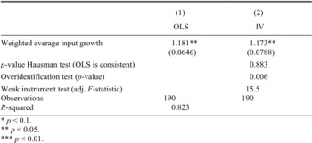
Table 1 shows the results from estimating equation 1, using ordinary least squares (OLS) in column 1 and using two-stage least squares based on instrumental variables (IV) in column 2.Footnote 44 Column 1 shows significant increasing returns to scale of 1.181, implying that a one percent change in inputs is accompanied by a 1.181 percent change in output. Note that the asterisks denote the statistical significance of the coefficients compared to the null hypothesis of constant returns to scale, i.e., a coefficient of one. Industry fixed effects are included but not shown in Table 1. Instead, the online appendix shows the fixed effects, which measure the period average technology change of each industry, alongside average Solow residual TFP growth, which assumes returns to scale are constant.45
Column 2 of Table 1 presents the results where we have used the change in oil price, real government expenditure, lagged real government expenditure, the currency-deposit ratio, and real deposits of failed banks as instruments that reflect industry demand but are not correlated with possible technology shocks. The estimates of returns to scale are very similar to the OLS estimates in column 1. A Hausman test can be used to determine whether there is a statistically significant difference between the ordinary least squares (OLS) and the instrumental variable (IV) regressions and this test shows no statistically significant difference (p = 0.883). So, the Hausman test confirms OLS as the best efficient estimator of the model.Footnote 46
For establishing the robustness of our returns to scale estimates, we considered alternative data choices, such as different input and output measures. We also tested whether there is heterogeneity in returns to scale across different groups of industries, such as between capital-intensive or durable-goods producing industries and noncapital intensive or nondurable industries. The results, shown in the online appendix, display little or no sensitivity to alternative input and output measures and no statistically significant differences across industry groups.
Testing the Real Business Cycle Hypothesis
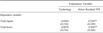
The key test of the RBC model and of a possible technology shock setting off the Great Depression is whether exogenous technology changes have had a positive and significant relationship with overall inputs and total hours worked. Table 2 reports the main results of this test. In the first column, labeled “Technology,” the technology residuals from the IV regression from column 2 of Table 1 have been used as the explanatory variable. This is the residual defined in equation 1 and any increasing returns to scale, due to labor hoarding, for example, are excluded from this technology measure. The measure in the second column, labeled “Solow residual TFP,” assumes constant returns to scale, so includes both technology change and increasing returns to scale. We have used the IV residuals rather than the OLS residuals since the OLS residuals are by construction (contemporaneously) uncorrelated with the explanatory variables.Footnote 47 Each row in the table indicates a different dependent variable, so each element in the table represents a separate regression.
THE EFFECT OF TECHNOLOGY CHANGE AND SOLOW RESIDUAL TFP CHANGE ON INPUTS IN U.S. MANUFACTURING, 1919–1939

* p < 0.1.
** p < 0.05.
*** p < 0.01.
Notes:
Robust standard errors, clustered by industry, are in parentheses. Each cell in the table represents a separate regression with one dependent variable and one explanatory variable. Dependent variables are either total inputs (weighted average growth of inputs) or growth of total hours. Explanatory variables are either technology change, the residual from the IV regression in column 2 of Table 1; or Solow residual TFP change, which is the growth of output minus weighted average growth of inputs.
Sources:
See the text.
The rows labeled “Total inputs” and “Total hours” of Table 2 cast serious doubt on the RBC hypothesis for the interwar period. Changes in Solow residual TFP are associated with large and statistically significant procyclical changes in inputs while a change in technology has no statistically significant effect on inputs. RBC theory predicts a positive relationship between each measure of technological change and inputs, so the absence of a statistically significant effect contradicts RBC theory. Compared to the findings of Basu, Fernald, and Kimball, we do not find a significantly negative relationship between technology and inputs, but this may well be due to the biennial nature of our data. Basu, Fernald, and Kimball find a significant negative effect in year one and a significant positive effect of similar magnitude in year two. Summed over the first two years of their regressions, the effect of technology change on inputs is therefore about zero, as in our results.48 We also verified whether these results are robust to adding lagged technology change and Solow residual TFP growth as Basu et al. did and those results were consistent with the findings from Table 2.Footnote 49
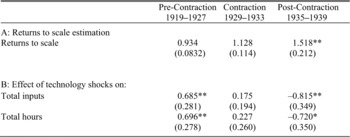
Much of the analysis of Cole and Ohanian focuses specifically on the depth of the Depression, 1929–1933. To rule out that statistical patterns for the full 1919–1939 period in Tables 1 and 2 are misleading for the Great Contraction years, we split our sample into pre-Contraction (1919–1927), Contraction (1929–1933), and post-Contraction (1935–1939) years. The estimated returns to scale and the effects of technology shocks on inputs are shown in Table 3.Footnote 50 The results reveal a clear difference between the pre-Contraction period, where the point estimates suggest decreasing returns to scale, the Contraction period with a statistically insignificant estimate of increasing returns to scale, and the post-Contraction period with strongly increasing returns.51 As a result, the effect of technology shocks in the 1920s seems more in line with RBC theory, with significantly positive effects on inputs. However, the results for the periods 1929–1933 and 1935–1939 are inconsistent with the RBC view. Indeed, the results for the 1929–1933 period are most closely in line with those for the full period from Table 2.
RETURNS TO SCALE AND THE EFFECT OF TECHNOLOGY CHANGE BY PERIOD IN U.S. MANUFACTURING, 1919–1939

* p < 0.1.
** p < 0.05.
*** p < 0.01.
Notes:
Robust standard errors, clustered by industry, are in parentheses. In Panel A, the dependent variable is output growth; the explanatory variable is weighted average input growth. “Returns to scale” is the coefficient of weighted average input growth and asterisks denote whether this coefficient is significantly different from 1. Returns to scale are estimated using two-stage least squares with the change in the oil price, real government expenditure, lagged real government expenditure, the currency-deposit ratio, and real deposits of failed banks as instruments (compare column 2 of Table 1). In Panel B, the residuals from Panel A are used to explain (growth of) total inputs and total hours (compare Table 2). All regressions include industry fixed effects (not shown).
Sources:
See the text.
The main conclusion from the first part of the analysis is therefore that negative technology shocks in U.S. manufacturing played little role in causing the Great Depression. The measured short-run standard Solow residual does not reflect changes in technology in the Depression era, which is inconsistent with a key prediction of RBC theorists. However, this provides no clear-cut evidence for what is driving these increasing returns. It could be that utilization effects are important since those would be most relevant during the 1930s. This would support the argument of Field that labor productivity and Solow residual TFP are both procyclical because of involuntary hoarding of capital. Businesses, and especially capital-intensive industries, were unable to get rid of capital in a downturn.52 However, it could also signal that surviving firms enjoyed greater market power following New Deal measures that dampened competition. This brings us to the other main question, namely what is driving the increasing returns: market power and/or hoarding?
Increasing Returns: Market Power or Hoarding?
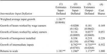
The output elasticities of individual inputs contain valuable information that can help us determine whether the increasing returns that we found were caused by market power or by labor and capital hoarding. Table 4 provides the results from estimating equation 5. Column 1 replicates the estimate from column 1 of Table 1, showing significant increasing returns to scale. Columns 2 and 3 replace weighted average input growth by the growth of the four inputs separately. In column 2, the coefficients of the input-deflated intermediate inputs (our preferred indicator) are displayed, while in column 3 output-deflated intermediate inputs are shown. Column 4 lists the cost shares of each input, averaged across branches and years. The bottom row shows returns to scale. For column 1, this is simply the coefficient on weighted average input growth. For columns 2 and 3, it is the sum of the output elasticities.
The returns to scale estimates are similar across the three specifications, implying increasing returns of about 20 percent. But new are the output elasticities and how they compare to the respective cost shares. For all these estimates we tested whether the output elasticity is equal to the actual cost share shown in column 4. For example, while the estimate of 0.181 in column 3 for the coefficient of growth of hours worked by wage earners is significantly larger than zero, it is not statistically significantly different from the actual cost share of wage earners, which is 0.169. Indeed, for none of the capital (horsepower installed) and labor (wage earners and salary earners) coefficients can we reject equality of output elasticity and cost share. However, the output elasticity of intermediate inputs (0.792 and 0.735) is statistically significantly larger than the cost share of 0.552. Should we focus only on the point estimates, it would imply that the output elasticity of intermediate inputs can account for all increasing returns. In terms of the patterns/hypotheses mentioned in Section 3, it means that we can reject the market power hypothesis, since that hypothesis predicts that all output elasticities would be larger than their cost share by the same factor. The results confirm the hoarding hypothesis since the coefficient of the intermediate inputs shows an output elasticity statistically significantly larger than its cost share, while the other input elasticities do not differ significantly from their cost share.Footnote 53 These results illustrate the importance of using a gross output framework. In a value added framework, intermediate inputs are assumed to have an impact on output that is in line with their cost shares. We show in Table 4 that this is not the case. Indeed, estimating production functions in a value added framework would lead to biased and misleading results.Footnote 54
RETURNS TO SCALE, OUTPUT ELASTICITIES, AND INPUT COST SHARES IN U.S. MANUFACTURING, 1919–1939

* p < 0.1.
** p < 0.05.
*** p < 0.01.
Notes:
Robust standard errors, clustered by industry, are in parentheses. The null hypothesis for weighted average input growth and returns to scale is that the parameter is equal to 1. In columns 2 and 3, returns to scale is the sum of the input coefficients. For other variables, the null hypothesis is that the parameter is equal to its cost share in column 4. Dependent variable in columns 1–3 is biennial growth of gross output in each of the 19 manufacturing industries between 1919 and 1939. Independent variable in column 1 is weighted average input growth based on total hours worked, horsepower installed, and input-deflated intermediate inputs. Column 2 includes input-price deflated growth of intermediate inputs and column 3 includes output-price deflated intermediate inputs. All regressions include industry fixed effects (not shown). Column 4 shows the average cost shares across industries and years of each input in total output. By assumption, the cost shares sum to one.
Sources:
See the text.
In the literature, many examples can be found of actual labor hoarding during the early 1930s. Bernanke explained the drop of the American workweek and the introduction of work-sharing as an efficient way for firms to react to falling demand. Firms cut production but at the same time the work force was left intact by spread-work schedules.Footnote 55 Robert Margo has argued that the legislation connected to the National Industry Recovery Act (1933–1935) promoted work-sharing provisions leading to the reduction in the length of the workweek.Footnote 56 A theoretical explanation is that especially skilled work might be viewed as a fixed factor in the short run. A certain part of the labor force acts as a buffer stock. Some labor that is normally used in production can be diverted into maintenance and repair operations during a recession.Footnote 57 Recently, Field has mentioned the important role of capital hoarding in explaining the procyclicality of Solow residual TFP. Holding existing capital is unavoidable and capital must be held by someone. Field's argument regarding capital hoarding implies that Solow residual TFP really did go down between 1929 and 1933 and it was not just a matter of mismeasurement. Capital service flows, in particular, were amortized over a much-reduced flow of output, so output per unit of input really did fall according to this interpretation.Footnote 58
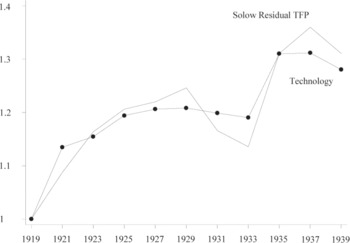
To see how large the impact of hoarding has been in manufacturing, we can illustrate the different time pattern of technology and hoarding in Figure 1.
SOLOW RESIDUAL TFP VERSUS TECHNOLOGY INDEX, WEIGHTED AVERAGE FOR TOTAL U.S. MANUFACTURING, 1919–1939

The Solow residual estimate of TFP growth for each industry is calculated as the growth of output minus the weighted growth of intermediate inputs, labor, and capital assuming constant returns to scale. Technological change is calculated as the growth of output minus 1.181 times inputs, where 1.181 is the returns to scale factor estimated in Table 1. We used value added shares to get a weighted average growth for overall manufacturing and turned this into an index with 1919 = 1.
Both series show the same overall pattern. Over the total period, the estimates suggest a rise in TFP of 28 to 31 percent between 1919 and 1939. But there are large differences in the variation of the series in individual periods, notably in 1920/21, the Great Contraction between 1929 and 1933, and the 1937 contraction. In the 1920/21 slump, Solow residual TFP grew at a slower rate than technology, while in the last two periods Solow residual TFP showed larger drops than technology. Our analysis has shown that this difference can be explained by hoarding effects. Between 1933 and 1937, however, Solow residual TFP is growing much faster than technology, because of massive expansion in the utilization of capital and labor.
Focusing on the period 1929–1933, technology dropped by only 1.5 percent, compared with an 8.9 percent fall in Solow residual TFP. Each decline is too small to explain the deep fall of output in the Depression, but each still shows declines. In part, this may reflect that “true” returns to scale will vary by industry and period, compared to our common scale factor, but it may also reflect firm dynamics. While we label our series “technology,” in line with e.g., Basu, Fernald, and Kimball, manufacturing industry consists of many firms and the technology series for each industry will be affected by within-industry firm dynamics. Recently, Amil T. Petrin, Kirk White, and Jerome P. Reiter analyzed firm dynamics in U.S. manufacturing for the 1977– 1996 period.Footnote 59 They show how aggregate technological change can be decomposed into contributions from firm technological change in the form of pushing out the production frontier and reallocation of resources between firms with different productivity levels. They find that the reallocation effects are negative during recessions in their sample period, while they are positive in other years. By comparison, technological change shows a more varied pattern that is also most often positive. Still, the findings suggest that changes in market shares of firms with different productivity levels may depress industry or manufacturing technology even in periods when underlying firm technology is improving.
Evidence for the interwar period on distinguishing firm dynamics and technological change is more scattered. There are many documented examples of disembodied technological change through the improvement of plants.Footnote 60 Although these developments varied considerably across industries, they also continued during the Depression. It is more challenging to establish the role of firm dynamics, the productivity levels of firms, and how their size varied throughout this period.61 Timothy Bresnahan and Daniel Raff perform such an analysis for the motor vehicle industry, using the Biennial Census of Manufactures data between 1929 and 1935.Footnote 62 They establish that there are two forces at work. First, firms remaining in business experienced large declines in output and relatively smaller declines in employment. This led to a decline in measured labor productivity and the difference in the rates of decline suggest labor hoarding. The second force is the entry of more productive new firms and the exit of less productive old firms. A third force that might have operated but was not important in the motor vehicle industry was shifts in market share between firms that remained in business. The net result of these forces in the motor vehicle industry was an increase in output per man-hour. We do not know the effects on industry technological change due to missing capital data in the Bresnahan and Raff study. However, this net result may well have come out differently in other industries. Indeed, widespread bank failures during the Depression may have cut off credit to low and high productivity firms alike, distorting the market mechanism that would normally have favored highly productive firms.Footnote 63 This remains a potentially fruitful area for further research.
CONCLUSIONS
The driving force behind recessions remains a topic of great interest and for the Great Contraction in the United States in particular. In this article, we have aimed to determine whether technology shocks are likely to have played an important role during this episode. Following a strict version of real business cycle (RBC) theory, the answer would be that technology shocks are the only driving force. This strict version is not a commonly held view, but a number of authors claim that technology shocks played a major role. Our findings suggest that this was not the case.
We construct an industry productivity data set covering all of manufacturing across 19 branches for the period 1919–1939. This data set includes all the variables that are commonly used for productivity analysis: output, intermediate inputs, capital (horsepower installed), and labor (wage earners and salary earners). To establish the role of technology shocks, we estimate industry production functions and find robust evidence of increasing returns to scale. We use the residuals from these production functions, our measure of “purified” technology change, to test a central prediction of RBC theory, namely whether technological change is positively correlated with input use such as total hours worked. The methodology follows that of Basu, Fernald, and Kimball for the postwar U.S. period. We find very similar results for the interwar period. Over a two-year time horizon, technology change has no statistically significant positive relationship with inputs. This finding is robust to a wide range of alternative specifications of the production function. These findings suggest that even the weaker version of RBC theory, namely that technology shocks played a role alongside other supply-side shocks, such as distortionary taxes or government supply side policies, is not supported.Footnote 64
There is little role for technology shocks in driving the Depression because the results show increasing returns to scale in manufacturing industries. As a result, Solow residual TFP change is mismeasured since that measure assumes constant returns to scale. Returns to scale might have been increasing because manufacturing firms had market power or because they hoarded labor and capital during downturns. We find clear evidence in favor of labor and capital hoarding and no evidence pointing to market power. We therefore conclude that the hoarding of production factors was the dominant reason for the decline in measured Solow residual TFP in U.S. manufacturing between 1929 and 1933. That still leaves important issues for future research: in particular the Depression's effect on firm-level dynamics in entry, exit, and changes in market shares and the relationship between dynamic changes and the adoption of new technologies.
Appendix 1: Data Sources and Methods
This appendix describes the methods used to construct the data set. We explain in more detail how we arrived at the hourly wage rates used to calculate the total number of hours worked for each branch. Additionally, the census data on capital—or to be more precise—on horsepower of installed machinery does not cover all years for the period under investigation. Therefore, we also explain the methods applied to calculate biennial capital data. Appendix Table 1 shows the 19 separate branches of manufacturing distinguished in this article. Together, they cover total manufacturing. The complete data set can be found in the online appendix.
INDUSTRY LIST AND CLASSIFICATIONS

Notes:
“Bernanke/Parkinson” indicates whether (part of) this industry was covered in the sample of Bernanke and Parkinson, “Procyclical”; “Capital-Intensive” indicates whether an industry is on average in the top half of the capital-output distribution; and “Durable” indicates whether the BEA currently classifies this industry as part of durable manufacturing in its GDP by Industry accounts.
Wages and Hours Worked
The wage data in the article come from three sources. For the period 1933–1939 data from the U.S. Department of Labor, Monthly Labor Review (MLR) were used for some 100 selected industries. From this monthly data, annual averages were calculated for each industry. The industries were matched with census industries and the numbers of wage earners working in these industries were added. Using employment as weights, the approximately 100 industries were then classified into the 19 branches presented here.
The MLR did not collect hourly wage rates prior to 1933. However, index numbers are available for the entire period. Woytinsky and Associates present index numbers on hourly earnings from 1919 to 1939 for 38 industries based on data from the Bureau of Labor Statistics.Footnote 65 Again, we matched these industries with census industries and summed over the total number of employees available from the census. Employment in these industries covers close to 50 percent of the entire manufacturing sector. The index series of the individual industries were aggregated to the branch level, using the census's employment of wage earners as weights. For the Machinery branch, Woytinsky and Associates present index numbers on agricultural implements and machinery only, which constitute between 3 and 5 percent of the total branch. Therefore, other sources have been employed to increase coverage in this branch.
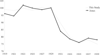
WEEKLY WORKING HOURS IN TOTAL U.S. MANUFACTURING, 1919–1939 (1929 = 100)

The National Industrial Conference Board (NICB) collected hourly wages for a selection of industries as well. Following the same procedure as with the other two data sources, these industries were matched to census industries and their hourly wages aggregated to branch level using industry wage earner employment as weights. The NICB data were used to provide additional coverage for the Machinery branch.
To arrive at hourly earnings for each of the 19 branches, we employed a combination of the sources described above. For the years 1933–1939 the data from the Monthly Labor Review were used. To calculate hourly wages for 1919 to 1931, the growth of the indices found in Woytinsky and Associates was used together with the levels of 1933 for each branch. For the Machinery branch, the level data of the NICB were taken for the period between 1921 and 1929, due to its superior coverage of industries in the Machinery branch. To calculate the wages in Machinery for 1929 and 1931 the growth of the index for Transportation Equipment was used. Average hourly wages for total manufacturing were calculated from the individual branches, using the total number of wage earners from the census in each branch as weights to ensure consistency. The MLR does not provide hourly wages for any industries in the Miscellaneous Industries branch, nor do any of the other sources used. Therefore, the weighted average hourly wage rate of total manufacturing was used as a proxy for the wage rate in this branch.
From the data on total wages paid in the census and the hourly wages at the branch level, total hours worked in each branch can be calculated. In Appendix Figure 1, we compare our results for the total manufacturing sector with the estimates of Ethel Jones to provide a reference.Footnote 66 Jones produced estimates of the average number of hours worked per week for wage earners in manufacturing, corrected for time spent on holidays and sick leave. The resulting values on hours worked reflect the time spent by workers on the job, not the time paid for by employers. The data on hours worked in the present study are calculated by dividing the total wages paid by an hourly wage rate for each industry. Therefore, these data must be interpreted as hours paid for, not hours spent on the job, since no adjustments for holidays and sick leave were made as was done in the study of Jones. In order to compare our series with Jones's, we divided our data on total hours worked at the total manufacturing level by the total number of wage earners and subsequently divided this number by 52 to arrive at the average number of hours paid for per person per week. The two data series on average weekly hours were converted to an index, with reference year 1929, to provide a comparison of the growth trend over time. Appendix Figure 1 shows that the growth rate of the numbers calculated in this article follow the trend of Jones's data quite closely at the total manufacturing level. It needs to be noted that we only used logarithmic growth rates in the regression estimates. Note, that both series display a sharp drop in hours of 25 percent between 1929 and 1935.67
Additionally, data on the number of salaried workers and salaries paid were gathered from the census data. As no hourly wage rates were available for salaried workers, we have put the average number of hours worked by a salaried worker equal to the average number of hours worked by a wage earner.
Capital
We constructed an annual capital stock series at the disaggregated level using the investment series by Dewhurst et al. and a perpetual inventory method to estimate stocks.Footnote 68 We found that annual depreciation rates averaging 45 percent were needed to arrive at the benchmark capital stock estimates by Creamer, Dobrovolsky, and Borenstein.Footnote 69 This suggests that the benchmark capital estimates and the investment series are inconsistent. As an alternative method, we used perpetual inventory method estimates from the 1919 benchmark with an arbitrarily established depreciation rate of 15 percent. However, as was noted in the article and shown in the online Appendix, the overall conclusions are not sensitive to the capital stock estimates.
Census horsepower (HP) statistics were available for 1919, 1923, 1925, 1927, 1929, and 1939. Therefore, data for the other census years had to be estimated. We did not simply interpolate linearly but tried to take cyclical variations into account. This was done in the following way: Value Added (VA) minus Total Wages paid (TW) was calculated and deflated with the deflator of the Machinery branch. The result (VA–TW) was taken as a proxy for gross investment. To calculate the level of horsepower for an industry for a particular year, the difference in the level of horsepower of the surrounding years was measured. We added to this value a depreciation of horsepower, which was calculated by multiplying horsepower in the year prior to the year(s) lacking data by a flat biennial depreciation rate (Δ) of 10 percent times the number of missing observations in between. Sensitivity analysis using alternative depreciation rates did not change the results. This gives a measure of change in horsepower between the years surrounding the missing data. Then we added the (VA–TW) values of all intervening years plus the end year for which data are available. Dividing the change in horsepower by this number gives the amount of horsepower per unit of (VA–TW) for each branch, which will be referred to as (R). This number is used to calculate the value of horsepower in the intervening years. Calculating forward from the year prior to the missing data, horsepower for each intervening year can be calculated by

Alternatively (HP)t can also be calculated backwards from the year after the missing data using
![\[
\begin{array}{c}
HP_{t} =\frac{1}{1-\delta }\left[{HP_{t+1} -R\left({VA-TW} \right)_{t} } \right]
\end{array}
\](https://static.cambridge.org/binary/version/id/urn:cambridge.org:id:binary:20160921005858766-0085:S0022050711002166:S0022050711002166_eqn9.gif?pub-status=live)
Using both methods produced two estimates for each year. As the last (first) year for which data is available can also be estimated in this way, we were able to see whether this estimation led to a bias. Typically, calculating forward yields a downward bias in the last year and calculating backward yields an upward bias for the first year. To offset these, a weighted average was calculated, with weights decreasing with the number of years from the starting year from which is calculated.
These results are dependent on the depreciation rate that is chosen. In this case we based it on an average asset lifetime of 20 years. However, experimenting with other depreciation rates showed that increasing the depreciation rate works to reduce the growth in horsepower installed in the early years of the depression and increases it in the second part of the 1930s for branches experiencing slow to moderate growth in terms of horsepower installed. For fast growing branches with respect to horsepower installed, we find the opposite.