

INTRODUCTION
Human populations are growing along coastlines, as well as the corresponding anthropogenic impact on their natural communities. Gathering accurate information on benthic communities is therefore urgently needed for the proper management and conservation of coastal ecosystems (Bertness, Reference Bertness1999). The exploitation of penaeid coastal shrimps in tropical regions is a very ancient activity that resulted in the current overexploitation of much of the fishery resources (Garcia & Le Reste, Reference Garcia and Le Reste1981). The impact of shrimp fisheries in tropical regions has become comparable to the world's most intensively exploited temperate shelf ecosystems, thus causing significant losses in spawning biomass and biodiversity, especially as a consequence of stocks trawling on soft-bottoms (Pauly & Christensen, Reference Pauly and Christensen1995; Pauly et al., Reference Pauly, Christensen, Guénette, Pitcher, Sumaila, Walters, Watson and Zeller2002).
Shrimp fisheries in south-eastern Brazil target the most profitable species, such as the pink shrimp Farfantepenaeus brasiliensis (Latreille, 1817) and F. paulensis (Pérez-Farfante, 1967), the white shrimp Litopenaeus schmitti (Burkenroad, 1938) and the seabob shrimp Xiphopenaeus kroyeri (Heller, 1862) (Costa et al., Reference Costa, Fransozo and Pinheiro2004; Castro et al., Reference Castro, Costa, Fransozo and Mantelatto2005). The recent increase in the fishing fleet and the decrease in landings of those species have contributed to the incorporation of additional species into those fisheries, including Artemesia longinaris Bate, 1888 and Pleoticus muelleri (Bate, 1888) (D'Incao et al., Reference D'Incao, Valentini and Rodrigues2002; Costa et al., Reference Costa, Fransozo and Pinheiro2004, Reference Costa, Fransozo, Castilho and Freire2005, Reference Costa, Fransozo, Freire and Castilho2007; Castilho et al., Reference Castilho, Costa, Fransozo and Boschi2007a). Other penaeoidean species that are habitually found in this region, such as the sicyoniids Sicyonia dorsalis Kingsley, 1878, and S. typica Boeck, 1864 and the penaeid Rimapenaeus constrictus (Stimpson, 1874), are still non-commercial species due to their small size.
Most shrimp species are found in tropical and subtropical regions, with a marked decrease in number towards temperate and cold regions. Their distribution may depend on a variety of environmental factors (Boschi, Reference Boschi2000). Several studies have investigated how the distribution of penaeid shrimps is modulated by variation in ecological parameters, particularly the type of sediment, salinity, depth and temperature (Fransozo et al., Reference Fransozo, Costa, Mantelatto, Pinheiro, Santos, Briones and Alvarez2002, Reference Fransozo, Costa, Castilho and Mantelatto2004; Costa & Fransozo, Reference Costa and Fransozo2004; Costa et al., Reference Costa, Fransozo and Pinheiro2004, Reference Costa, Fransozo, Castilho and Freire2005, Reference Costa, Fransozo, Freire and Castilho2007; Castro et al., Reference Castro, Costa, Fransozo and Mantelatto2005). However, little is known about how these ecological parameters translate into the abundance patterns at the level of entire shrimp communities. Such knowledge is fundamental, not only to understand the mechanisms underlying shrimp community dynamics, but also to effectively manage shrimp fishery resources.
The goal of the present study is to understand how variation in environmental characteristics affects the abundance patterns of shrimp communities on the south-eastern coast of Brazil using multivariate methods.
MATERIALS AND METHODS
Shrimp collections were carried out monthly between July 2001 and June 2003 in two locations—Ubatuba (UB) and Caraguatatuba (CA)—both on the northern coast of the state of São Paulo, south-eastern Brazil (UB: −23°26′27′′ −45°03′18′′; CA: −23°36′09′ −45°20′25′′). Seven transects were sampled in each location at varying depths (5, 10, 15, 20, 25, 30 and 35 m). A shrimp-fishing boat equipped with two double-rig nets (mesh size 20 mm and 15 mm in the cod end) was used for trawling, which lasted for 30 minutes in each transect, sampling a total area of approximately 18,000 m2. When a given trawl yielded considerable biomass of a given species, a 200 g random subsample of that species was obtained and examined separately, and the results were extrapolated for that respective species in that trawl.
Five environmental characteristics were recorded at each location, namely: bottom water salinity and temperature, organic matter content, depth, and sediment grain size. A detailed description of the sampling methods and an analysis of environmental parameters during the study period are available elsewhere. Bottom water was sampled using a Nansen bottle. The salinity was measured with an Atago S/1000 optic refractometer, whereas the temperature (°C) was measured using a thermometer attached to the bottle. An ecobathymeter coupled with a GPS was used to record depth (m) at sampling sites. Sediment samples were collected at each station with a Van Veen grab (0.06 m2). In the laboratory, the sediment was dried at 70°C for 72 h. For the analysis of grain size composition, two 50-g sub-samples were treated with 250 mL of a NaOH 0.2 N solution, stirred for five minutes to release silt and clay particles, and then rinsed on a 0.063-mm sieve.
Sediments were sieved through 2 mm (gravel); 2.0–1.01 mm (very coarse sand); 1.0–0.51 mm (coarse sand); 0.50–0.26 mm (medium sand); 0.25–0.126 mm (fine sand); and 0.125–0.063 mm (very fine sand); smaller particles were classified as silt–clay. Grain size categories followed the American standard, and fractions were expressed on the phi (φ) scale, i.e. using the formula φ =−log2d, where d = grain diameter (mm) (Tucker Reference Tucker1988), e.g. −1 = φ <0 (very coarse sand); 0 = φ < 1 (coarse sand); 1 = φ < 2 (intermediate sand); 2 = φ < 3 (fine sand); 3 = φ < 4 (very fine sand) and φ ≥ 4 (silt + clay). Finally, φ was calculated by cumulative particle-size curves plotted on a computer using the φ scale, with values corresponding to the 16th, 50th and 84th percentiles being used to determine the mean diameter of the sediment using the formula Md = (φ16 +φ50 + φ84)/3. Finally, φ was calculated.
The organic matter content (%) was obtained by ash-weighing: 3 aliquots of 10 g each per transect were placed in porcelain crucibles, heated for 3 h at 500°C, and then weighed again.
The relationship between the environmental factors and the abundance patterns in the shrimp communities was assessed using a canonical correlation analysis (CCorrA). This analysis is a multivariate statistical procedure that directly measures the strength of relationships between two sets of variables. The first set of variables used during the CCorrA included the environmental characteristics (bottom water salinity and temperature, organic matter content, depth, and φ), whereas the second set of variables included the abundance of the studied species (L. schmitti, R. constrictus, S. dorsalis, P. muelleri, A. longinaris, F. brasiliensis, F. paulensis and X. kroyeri). Sicyonia laevigata Stimpson, 1871 and S. typica were also recorded in the study areas, yet were not incorporated into the CCorrA because they were present in less than 10% of the monthly samples in either site (Cuesta et al., Reference Cuesta, González-Ortegón, Rodríguez, Baldó, Vilas and Drake2006).
Three alternative data transformations were tested with respect to their capacity to improve the normality of the data: 1/x, ln(1 + x), and sqrt(x), and the most appropriate transformation was chosen based on the lowest Kolmogorov–Smirnov D. Using this criterion, the abundance of R. constrictus, S. dorsalis, P. muelleri, F. brasiliensis, and X. kroyeri was sqrt-transformed, whereas the abundance of A. longinaris and the levels of organic matter were ln-transformed prior to the analyses. However, it is important to point out that CCorrA is fairly robust to violations in this assumption, and an analysis of the same dataset with untransformed variables provided similar results, except for a slightly lower fit of the model to the data (not shown).
All samples from both locations were incorporated into the same analysis. This approach is justified given that the goal of the present study is not to characterize each sampling location. Instead, by including the widest possible variation in environmental parameters, one would expect that the effects of these parameters on the shrimp communities would become more apparent.
RESULTS
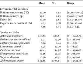
Variation in the environmental parameters and in species abundance is shown in Table 1. The range of variation recorded during this study is likely to encompass most of the conditions found throughout the geographical range of the studied species.
Observed variation in the environmental variables and in the number of captured individuals of each species in the present study.

SD, standard deviation.
A total of 374,915 individuals were collected during the present study. Xiphopenaeus kroyeri showed the highest abundance (273,127 individuals), followed by A. longinaris (73,422 individuals) and P. muelleri (15,262 indoviduals), with each of those three species accounting for 73%, 20%, and 4% of all captured individuals, respectively.
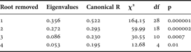
The CCorrA resulted in a canonical correlation coefficient of 0.59 (P < 0.000001), with 100% of the variance being extracted from the dataset of the environmental variables (total redundancy of 23.02%), whereas 69.35% of the variance was extracted from the dataset with information on the community composition (total redundancy of 12.07%). The first four roots were statistically significant (Table 2). However, the first canonical root accounted for more than three times the explained variance than the second root (27.3 % and 8.6 %, respectively), with little difference in the explained variance between roots 2 and 4.
Results of canonical correlation analysis of shrimp communities in south-eastern Brazil. See text for details.

df, degrees of freedom.
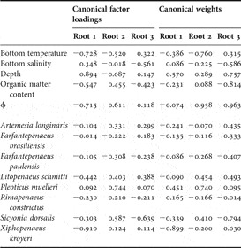
The canonical factor loadings (the correlation between the canonical and the original variables) and the canonical weights (the partial correlations of the original variables with respect to the canonical root) for the first three roots are shown in Table 3. The environmental variable with the highest factor loading in the first root is depth (0.89), followed by φ and temperature, which show similar loadings of opposite signs in relation to depth (−0.71 and −0.72, respectively). However, given the high level of covariance among these variables, an inspection of their canonical weights can provide an indication of their individual contributions controlling for other variables. Indeed, the factor loading of φ seems to be best explained by covariance with other variables, with little direct contribution to the variation in the dataset (CWφ = −0.07). On the other hand, both depth and temperature show high and opposite canonical weights, indicating that the first root reflects most strongly the variation in these two variables.
Canonical factor loadings and weights based on the canonical correlation analyses of the relationship between environmental characteristics and shrimp abundance patterns.

The second root reflects an inverse relationship between φ and bottom temperature, as shown by their high factor loadings (0.61 and −0.52, respectively), and specially their canonical weights (0.96 and −0.76, respectively). Finally, the third root reflects an inverse relationship between φ and organic matter content, with the latter showing a canonical weight of −0.81.
There was little consistency in the response of the studied shrimp species to variation in environmental variables. The first root was strongly associated with the abundance of X. kroyeri, as revealed by its high factor loading (−0.91) and canonical weight (−0.89), yet no other species showed values more extreme than±0.5 for either statistic. Similar associations were found between P. muelleri and root 2, and between S. dorsalis and root 3. Interestingly, the variation in abundance of L. schmitti, R. constrictus, A. longinaris, F. brasiliensis and F. paulensis were not well-described by any of the first three roots in the model.
DISCUSSION
Benthic communities are affected by a variety of biotic and abiotic parameters, including sea floor characteristics, food availability, tidal and sea-level patterns, community composition, prey–predator relationships, interactions among species, and the reproductive strategies of their component species (Lenihan & Micheli, Reference Lenihan, Micheli and Bertness2001). These ecological variables are reflected in the evolutionary adaptations of species and their large-scale biogeographical patterns (Harley et al., Reference Harley, Hughes, Hultgren, Miner, Sorte, Thornber, Rodriguez, Tomanek and Williams2006). The biogeographical provinces of the south-western Atlantic Ocean begin at latitudes 43–44° S, spanning the continental shelves of Argentina, Uruguay and southern Brazil. On the other hand, the coastal region between 23° and 35° S is a transitional area characterized by processes of mixing and instability of the water masses, with presence of both eurythermal and euryhaline species (Boschi, Reference Boschi2000).
The south-eastern Brazilian coast is strongly affected by two water masses: the Coastal Water (CW) and Tropical Water (TW). The effects of these water masses are more pronounced during autumn and winter, when temperature and salinity levels increase to over 21°C and 35, respectively. Another water mass, the South Atlantic Central Water (SACW), intrudes throughout late spring and summer, causing decreases in temperature (<20°C) and bottom salinity (<35). The incursion of the TW into the uppermost water layers and the dislocation of the CW towards the ocean during the autumn and winter cause vertical mixing and thus eliminate the existing seasonal thermocline, causing the SACW to recede towards the offshore region (Castro-Filho et al., Reference Castro-Filho, Miranda and Myao1987; Castilho et al., 2007a, b). The intrusion of the SACW causes considerable changes to the resident communities, either positive or negative. Some species show abundance peaks associated with the arrival of the SACW, as in the case of the crabs Portunus spinicarpus (Stimpson, 1871), Leurocyclus tuberculosus (Edwards & Lucas, 1843) and Stenocionops spinosissima (Saussure, 1857). Therefore, the south–south-east shelf represents an area of intense faunistic transition, including species ranging from tropical to subantarctic (Boschi, Reference Boschi2000).
In addition to corroborating the scenario described above, our results indicate that variation in the abundance of X. kroyeri and P. muelleri was influenced by variation in temperature. The influence of the SACW (cold waters = 15°C) for X. kroyeri is responsible for a decrease in the number of collected individuals. Similar results were found by Fransozo et al. (Reference Fransozo, Costa, Mantelatto, Pinheiro, Santos, Briones and Alvarez2002), Castro et al. (Reference Castro, Costa, Fransozo and Mantelatto2005) and Costa et al. (Reference Costa, Fransozo, Freire and Castilho2007), suggesting that temperatures below 21°C may be limiting for this species. The inverse relationship of abundance and temperature was verified to P. muelleri, which together with A. longinaris, can be considered as indicator species of the inbound cold water (Boschi, Reference Boschi1969, Reference Boschi1989; Gavio & Boschi, Reference Gavio and Boschi2004; Fransozo et al., Reference Fransozo, Costa, Castilho and Mantelatto2004; Costa et al., Reference Costa, Fransozo and Pinheiro2004, Reference Costa, Fransozo, Castilho and Freire2005). Although both species migrate to the south-western shore of Brazil during the intrusions of the SACW, the present study found little association between temperature and the abundance of A. longinaris. These results corroborate the hypothesis of Costa et al. (Reference Costa, Fransozo, Castilho and Freire2005) that A. longinaris can cope with more pronounced thermal oscillations and migrates farther north along the Brazilian coast than P. muelleri.
Several authors have suggested that the distribution of penaeoid shrimps is strongly modulated by the texture and the organic content of the substrate (Boschi, Reference Boschi1969; Dall et al., Reference Dall, Hill, Rothlisberg, Staples, Blaxter and Southward1990; Nakagaki et al., Reference Nakagaki, Negreiros-Fransozo and Fransozo1995). However, those factors did not exert a consistent influence on the studied community as a whole. Although the second root indicated an inverse relationship between φ and bottom temperature and the third root reflected an inverse relationship between φ and organic matter content, most species showed weak loadings on those roots, except for P. muelleri and S. dorsalis on the first and second roots, respectively.
The abundance patterns of X. kroyeri and P. muelleri were strongly affected by water depth, but in different directions: X. kroyeri was observed in shallow waters, whereas P. muelleri was more characteristic of higher depths. A similar result was obtained by Costa (Reference Costa2002) in the Ubatuba region, where 95% of the captures of X. kroyeri were carried out in inshore waters (depth ≤15 m). Also, Costa et al. (Reference Costa, Fransozo and Pinheiro2004) observed a positive association between the abundance of P. muelleri and water depth in the Ubatuba region, with most captures occurring at depths greater than 9 m. According to Castro-Filho et al. (Reference Castro-Filho, Miranda and Myao1987), CW can affect shallow waters up to 25 m in depth. In this water mass, salinity is always below 36 and temperature above 20°C. Also, the SACW can lead to a temperature decrease in deeper areas, occasionally reaching more coastal grounds. Thus, the inverse abundance variation for depth of these species might reflect bathymetric variation in temperature, a clear example of distinct behavioural differences of species of different origins, either tropical (X. kroyeri) or subantarctic (P. muelleri). Thus, depth and temperature were among the main factors underlying the abundance patterns of X. kroyeri and P. muelleri in the period and regions studied.
Two hypotheses are proposed to explain the low association between the remaining environmental factors and the abundance patterns of the studied species. First, it is possible that the amplitude of the variation in the environmental conditions was not sufficient to allow for their effects to be apparent. One such condition is salinity, given that the samples were only conducted in the marine environment. For instance, Gunter et al. (Reference Gunter, Christmas and Killebrew1964) showed a significant influence of salinity on shrimp abundance patterns in southern Texas by sampling salinity levels from 5 to 35. Alternatively, a general description of how shrimp abundance responds to environmental changes might not be realistic because each shrimp species may in fact display its own idiosyncratic environmental preferences and constraints.
Alternatively, variation in the abundance patterns of the studied species might result from the influence of other biotic and abiotic factors that were not considered in the present study, such as intraspecific migration patterns. According to Dall et al. (Reference Dall, Hill, Rothlisberg, Staples, Blaxter and Southward1990), juvenile and subadult shrimps of the species F. brasiliensis, F. paulensis and L. schmitti are most commonly found in inshore regions such as bays until they reach gonadal maturity, when they migrate to offshore regions during the breeding and spawning periods. It is important to note that, according to Chagas-Soares et al. (Reference Chagas-Soares, Pereira and Santos1995), the south littoral of São Paulo state (Cananéia region) is a rich nursery ground for the shrimp L. schmitti and Farfantepenaeus spp. Costa (Reference Costa2002) suggested that subadults of L. schmitti captured in Ubatuba had in fact immigrated from another region, such as Cananéia. Therefore, the variation in abundance of those species might at times be related to the physiological demands associated with their reproductive behaviour, such as the migration of adults for copulation and spawning, rather than to environmental factors responsible for the permancence of those species in the studied shores.
Penaeid shrimp in south-eastern Brazil also seem to adjust their reproductive phenology to variation in phytoplankton, particularly the increase in their abundance during the spring and summer resulting from the upwelling of the SACW (Costa & Fransozo, Reference Costa and Fransozo2004; Castilho et al., Reference Castilho, Costa, Fransozo and Boschi2007a, Reference Castilho, Gavio, Costa, Boschi, Bauer and Fransozob). In addition, the shrimp communities in the present study include both tropical and subantartic species (Boschi, Reference Boschi2000), which might display idiosyncratic responses to environmental factors and food availability. Future studies on habitat selection, focusing specifically on the spawning sites and the patterns of juvenile recruitment on the northern coast of São Paulo, are specially relevant to clarify the presented hypothesis on the relationship between environmental variation and the abundance of the studied species.
ACKNOWLEDGEMENTS
The authors are grateful to Fapesp, CNPq for financing part of this work, to the NEBECC members for helping during samplings and laboratory activities. We thank the Instituto Brasileiro do Meio Ambiente e dos Recursos Naturais Renováveis (IBAMA) for granting permission to collect the shrimps.