1 INTRODUCTION
Factor models have been widely used in economics and finance. In a factor model,
 $$ \begin{align} X_{it}=\lambda _{i}^{0\prime }F_{t}^{0}+e_{it}, i=1,\ldots ,N,t=1,\ldots ,T, \end{align} $$
where
 $X_{it}$
is the observed data for the ith individual at time t,
 $ F_{t}^{0}$
is an
 $r\times 1$
vector of latent factors,
 $\lambda _{i}^{0}$
is the corresponding
 $r\times 1$
vector of factor loadings, and
 $e_{it}$
is the idiosyncratic error with possible weak dependence across i or/and over t. Until very recently, a large body of literature on factor models has built on the assumption that all factors are strong in the sense that both
 $ T^{-1}\sum _{t=1}^{T}F_{t}^{0}F_{t}^{0\prime } $
and
 $N^{-1}\sum _{i=1}^{N} \lambda _{i}^{0}\lambda _{i}^{0\prime }$
converge to some positive definite (p.d.) matrices. However, the assumption of strong factors may fail due to the sparsity in loadings or many nonzero but small loadings. In such cases, we generally obtain a weak factor model, where
 $N^{-1}\sum _{i=1}^{N} \lambda _{i}^{0}\lambda _{i}^{0\prime }$
tends to be singular while
 $T^{-1} \sum _{t=1}^{T}F_{t}^{0}F_{t}^{0\prime }$
converges to a p.d. matrix. In this article, we focus on weak factor models with sparse loadings, i.e., sparsity-induced weak factor models.
Many empirical studies support the widespread existence of sparse factor loadings. For instance, both Stock and Watson (Reference Stock and Watson2002) and Ludvigson and Ng (Reference Ludvigson and Ng2009) find that the extracted PC factors from a large set of macroeconomic variables can fit the time-series observations of only a few variables well, suggesting a sparsity structure in loadings (see also Kristensen, Reference Kristensen2017; Freyaldenhoven, Reference Freyaldenhoven2022; Uematsu and Yamagata, Reference Uematsu and Yamagata2023a, Reference Uematsu and Yamagata2023b, UY hereafter). Moreover, hierarchical or group factor models, where factors have nonzero loadings only for some specific cross-sectional (CS) units or group, also echo the sparsity in loadings. For example, an oil supply shock only affects industrial production sectors but not others; size-sorted portfolios are influenced by the size factor, but momentum-sorted portfolios may not be. Additionally, weak factors may emerge as unsystematic risk due to market incompleteness (Dello-Preite et al., Reference Dello-Preite, Uppal, Zaffaroni and Zviadadze2024). For more examples of sparsity in loadings, see Ando and Bai (Reference Ando and Bai2017) and Choi, Lin, and Shin (Reference Choi, Lin and Shin2023).
When loadings are sufficiently sparse, what we encounter turns to be a weak factor model. A sparse weak factor only affects a small subset of individuals and the model with sparse weak factors is called “sparse weak factor model”.Footnote 1 The sparsity structure in loadings has attracted a lot of research interest. For example, Pelger and Xiong (Reference Pelger and Xiong2022) consider the sparse approximation to factor models, and Freyaldenhoven (Reference Freyaldenhoven2023) and Despois and Doz (Reference Despois and Doz2023) study the identification of factor models based on sparsity. In the presence of sparse weak factors, Giglio, Xiu, and Zhang (Reference Giglio, Xiu and Zhang2023) show that the prediction based on factor-augmented regression (FAR), a popular method for macroeconomic forecasting, is inconsistent (see also Chao and Swanson, Reference Chao and Swanson2022; Chao, Liu, and Swanson, Reference Chao, Liu and Swanson2022 for inconsistent prediction in factor-augmented vector autoregression [FAVAR]). Giglio, Xiu, and Zhang (Reference Giglio, Xiu and Zhang2025) show that in the 3-step estimation of risk premium in Giglio and Xiu (Reference Giglio and Xiu2021), sparse loadings raise a severe attenuation bias. For extremely weak factor models, Onatski (Reference Onatski2012) shows that the PC estimator is inconsistent.Footnote 2 For general weak factors, Bai and Ng (Reference Bai and Ng2023) re-investigate the asymptotics for principal component analysis (PCA) based on the singular value decomposition. In a linear regression framework with interactive fixed effects, such as in Bai (Reference Bai2009) and Su and Chen (Reference Su and Chen2013), Armstrong, Weidner, and Zeleneev (Reference Armstrong, Weidner and Zeleneev2025) show that when some factors are weak, previously developed estimators and confidence intervals (CIs) can be heavily biased. They subsequently propose improved estimators and bias-aware CIs that are uniformly valid, regardless of whether the factors are strong or weak.
To avoid the problems caused by sparse weak factors, two main solutions have been proposed. The first is to recover the sparsity in loadings using penalized regressions. UY (Reference Uematsu and Yamagata2023a) propose a sparse orthogonal factor regression (SOFAR) estimator using
 $\ell _{1}$
-regularization, and UY (Reference Uematsu and Yamagata2023b) further provide an inferential procedure to determine whether each loading component is zero while controlling the false discovery rate (FDR). The second solution is to pursue a strong factor model via screening out irrelevant individuals or variables. Giglio, Xiu, and Zhang (Reference Giglio, Xiu and Zhang2023, Reference Giglio, Xiu and Zhang2025) propose a supervised PCA method for two distinct purposes: selecting test assets to evaluate new factors and choosing predictors to forecast a target macroeconomic variable. By eliminating assets that lack exposure to the factor under evaluation or dropping predictors that are uncorrelated to the target variable, each factor within the model becomes strong. Similar ideas are also employed in Chao and Swanson (Reference Chao and Swanson2022) and Chao, Liu, and Swanson (Reference Chao, Liu and Swanson2022) in FAVAR.
Regularization-based approaches are often relatively complicated and carry heavy computational burdens due to the search of tuning parameters or the use of complex iterative algorithms. In contrast, we directly investigate the properties of the PCA method and propose recovering the sparsity in loadings via screening the PC estimator. Our article makes several contributions to the existing literature. First, we show the PC estimators for loadings are almost sparsity-preserving. To the best of our knowledge, ours is the first paper to reveal this intrinsic sparsity preservation feature of the PCA estimator for factor models. This finding contrasts sharply with the prevailing understanding that the sparsity of loadings cannot be preserved due to a matrix rotation (see Bailey, Kapetanios, and Pesaran, Reference Bailey, Kapetanios and Pesaran2021, BKP hereafter; Freyaldenhoven, Reference Freyaldenhoven2023). Second, given the near-invariance of sparsity and the consistency of PC estimators, we can easily recover the sparsity of loadings with proper screening to the PC estimator for loadings. The revelation of sparsity is important since it can lead to a better interpretation and understanding of, e.g., which factors are relatively important to which individuals. Another appealing advantage of our method is its negligible computational burden compared to regularization-based procedures. We only need to run standard PCA once and then apply our screening device directly to the estimated loadings. Third, based on the sparsified loading estimators, we can straightforwardly estimate distinct factor strengths and establish consistency of the strength estimators. Our approach allows for different factor strengths across factors, thereby improving BKP (Reference Bailey, Kapetanios and Pesaran2021), which only identify the strength of the strongest latent factor and require a complex sequential procedures. The estimated factor strengths can serve as valuable indicators for forecasting and policy-making. Fourth, for sparse weak factor models with varying sparsity degrees, we establish the large sample properties for the PC estimators of factors, loadings, and common components. Complementary to Bai and Ng (Reference Bai and Ng2023), we provide uniform convergence results for the PC estimates, which are useful for further analyses, such as constructing diffusion indices and factor-augmented instrumental variable regressions.
Finally, we need to mention the works most closely related to ours: UY (Reference Uematsu and Yamagata2023a) and Jiang, Uematsu, and Yamagata (Reference Jiang, Uematsu and Yamagata2024). UY (Reference Uematsu and Yamagata2023a) define a pseudo-true parameter as a representation of
 $\Lambda ^0$
and
 $F^{0}$
that satisfies
 $T^{-1}F^{0\prime }F^{0}=I_{r} $
and the diagonality of
 $\Lambda ^{0\prime }\Lambda ^{0}$
, even though this representation need not correspond to the true data-generating process (DGP). Jiang, Uematsu, and Yamagata (Reference Jiang, Uematsu and Yamagata2024) recently prove that such pseudo-true parameter always exists, thereby clarifying the estimand of the plain PC method. Our work provides a complementary perspective: while Jiang, Uematsu, and Yamagata (Reference Jiang, Uematsu and Yamagata2024) begin with the PC estimator and ask what pseudo-true parameter it consistently estimates, we begin with a sparse representation of the factor model and analyze whether the PC estimators inherit that sparsity in the loadings. Thus, both studies address the identification of PC estimators, but from fundamentally different angles.
The rest of this article is organized as follows. Section 2 formally introduces the sparse weak factor model, i.e., a weak factor model arising from sparse loadings, and the PC estimation method. In Section 3, we study the asymptotic properties of the PC estimators for factors, loadings, and common components under the weak factor framework, establishing their consistency, asymptotic distributions, and uniform convergence rates. Building on the result from Section 3 that the rotation matrix is approximately (block) upper triangular, we propose a screening method to sparsify the estimated loadings and provide consistent estimators for factor strengths in Section 4. Monte Carlo simulations are reported in Section 5, and Section 6 concludes. All technical proofs for the main results in Sections 3 and 4, as well as the determination of the number of factors, additional simulation results, and an empirical application, are relegated to the Supplementary Material.
Notations. For a set S, let
 $|S|$
be its cardinality. Let
 $a\vee b=\max \left \{ a,b\right \} $
and
 $a\wedge b=\min \left \{ a,b\right \} $
for two real numbers a and b. For two random sequences
 $\left \{ a_{n}\right \} $
and
 $ \left \{ b_{n}\right \}$
,
 $a_{n}\lesssim _{p}b_{n}$
denotes
 $a_{n}/b_{n} $
is stochastically bounded and
 $a_{n}\asymp _{p}b_{n}$
if
 $a_{n}\lesssim _{p}b_{n}$
and
 $b_{n}\lesssim _{p}a_{n}.$
When
 $\left \{ a_{n}\right \} $
and
 $ \left \{ b_{n}\right \} $
are deterministic
 $, a_{n}\lesssim b_{n}$
denotes
 $ a_{n}/b_{n} $
is bounded and
 $a_{n}\asymp b_{n}$
if
 $a_{n}\lesssim b_{n}$
and
 $b_{n}\lesssim a_{n}.$
For a square matrix A,
 $\mu _{\min }\left ( A\right ) $
and
 $\mu _{\max }\left ( A\right ) $
are the smallest and largest eigenvalues of A, respectively. Let
 $\left \Vert B\right \Vert =\left [ \text { Tr}\left ( BB^{\prime }\right ) \right ] ^{1/2}$
be the Frobenius norm of matrix B and
 $\left \Vert B\right \Vert _{sp}=\mu _{\max }^{1/2}\left ( B^{\prime }B\right ) $
be its spectral norm. For an
 $n\times 1$
vector a, its
 $\ell _{0}$
-norm is
 $\left \Vert a\right \Vert _{0}=\sum _{j=1}^{n}\mathbf {1 }\left ( a_{j}\neq 0\right ) $
, where
 $\mathbf {1}\left ( \cdot \right ) $
is the usual indicator function.
2 THE SPARSE WEAK FACTOR MODELS
2.1 The Definition of Sparse Weak Factor Models
In this article, we consider the following factor model with a sparse representation:
 $$ \begin{align} X_{it}=\lambda _{i}^{0\prime }F_{t}^{0}+e_{it}=\sum_{k=1}^{r}\lambda _{ik}^{0}F_{tk}^{0}+e_{it}, \end{align} $$
where
 $\lambda _{i}^{0}=\left ( \lambda _{i1}^{0},\ldots ,\lambda _{ir}^{0}\right ) ^{\prime }$
and
 $F_{t}^{0}=\left ( F_{t1}^{0},\ldots ,F_{tr}^{0}\right ) ^{\prime }.$
Footnote
3
In a matrix form, the model in (2.1) can be written as
 $X=\Lambda ^{0} F^{0 \prime }+e$
, where X and e are both
 $N\times T$
matrices with
 $X(i,t)=X_{it}$
and
 $e(i,t)=e_{it}$
, respectively,
 $\Lambda ^{0}=\left ( \lambda _{1}^{0},\ldots ,\lambda _{N}^{0}\right ) ^{\prime }$
and
 $F^{0}=\left ( F_{1}^{0},\ldots ,F_{T}^{0}\right ) ^{\prime }$
. We assume that the factors are well-behaved in the sense that
 $T^{-1} \sum _{t=1}^{T}F_{t}^{0}F_{t}^{0\prime }\rightarrow _{p}\Sigma _{F}$
as
 $ T\rightarrow \infty $
for some p.d. and finite matrix
 $\Sigma _{F}$
. For the kth factor,
 $k=1,\ldots ,r$
, the
 $\ell _{0}$
-norm of the
 $N\times 1$
factor loadings
 $\Lambda _{\cdot ,k}^{0}:=\left ( \lambda _{1k}^{0},\ldots ,\lambda _{Nk}^{0}\right ) ^{\prime }$
is of order
 $N^{\alpha _{k}}$
for some
 $\alpha _{k}\in \lbrack 0,1]$
, that is,
 $$ \begin{align} \left\Vert \Lambda _{\cdot ,k}^{0}\right\Vert _{0}=\sum_{i=1}^{N}\mathbf{1} \left( \lambda _{ik}^{0}\neq 0\right) \asymp N^{\alpha _{k}}. \end{align} $$
According to (2.2),
 $\alpha _{k}=1$
defines a strong factor which affects almost all CS units;
 $\alpha _{k}=0$
leads to an extremely weak factor which at most affects a finite number of units; any
 $ \alpha _{k}\in (0,1)$
gives a sparse structure on the N loadings. A larger
 $\alpha _{k}$
implies a stronger factor which affects more CS units. So the strength of the kth factor or the sparsity degree in its loadings can be represented by
 $\alpha _{k}$
. As BKP (Reference Bailey, Kapetanios and Pesaran2021), we define the parameter
 $\alpha _{k}$
as the factor strength of the kth factor. Further, we arrange the r factors in (2.1) by their factor strengths such that
 $ \alpha _{1}\geq \alpha _{2}\geq \cdots \geq \alpha _{r-1}\geq \alpha _{r}. $
A decreasing sequence
 $\left \{ \alpha _{k}\right \} _{k=1}^{r}$
can capture the sparsity structure of the factor models.
For any bounded and invertible rotation matrix
 $R\in \mathbb {R}^{r\times r}$
, we denote observationally equivalent factors and loadings as:
 $F=F^{0}R$
and
 $\Lambda =\Lambda ^{0}\left ( R^{\prime }\right ) ^{-1}$
. Consequently, we can define the factor strength vector for F, analogously to (2.2), as
 $\alpha \left ( R\right ) \equiv \left ( \alpha _{1}\left ( R\right ) ,\dots ,\alpha _{r}\left ( R\right ) \right ) ^{\prime }$
with
 $\alpha _{j}\left ( R\right ) \in \lbrack 0,1]$
for
 $j=1,\ldots ,r$
, and
 $\alpha _{j}\left ( R\right ) \geq \alpha _{k}\left ( R\right ) $
for
 $j<k$
. Due to the intrinsic identification indeterminacy of model (2.1), to characterize our sparse weak factor model with well-defined factor strengths, we introduce the following definition of the sparsest representation.
Definition 2.1 (The sparsest representations of a factor model).
The rotation matrix
 $R^{\ast }\in \mathbb {R}^{r\times r}$
gives a sparsest representation of factor loadings (up to order), if the factors after rotation
 $F^{*}=F^0R^*$
satisfy that
 $T^{-1}F^{*\prime }F^{*}$
is p.d. and finite in probability limit, and each element of factor strength vector
 $\alpha \left ( R^{\ast }\right ) $
cannot be further reduced for any other rotation matrix, that is
 $ \alpha _{k}\left ( R^{\ast }\right ) \leq \alpha _{k}\left ( R\right ) \text { for any invertible and bounded }R\in \mathbb {R}^{r\times r}\text { and } k=1,\ldots ,r. $
Remark 1. The sparsest representation indeed exists and is well defined. Definition 2.1 pins down uniquely the factor strengths for the sparsest representations, regardless of common or distinct factor strengths (or mixed of both). We will show that all factor strengths can be consistently estimated in Section 4.2. Here, we need to mention that the sparsest representation is not unique because many rotations give the same factor strengths vector
 $\alpha (R^{*})$
.
As discussed later in Section 3 with the relevant normalization in Assumptions 1 and 2 therein, it implies that the underlying
 $\left ( F^{0}, \Lambda ^{0} \right )$
has the sparsest representation with
 $R^{\ast }=I_{r}$
and factor strengths
 $\alpha \left ( I_{r}\right ) $
, where
 $I_{r}\in \mathbb {R }^{r\times r}$
is the identity matrix. In other words, there is no other rotation matrix that can further reduce any element of the factor strength vector
 $\alpha \left ( I_{r}\right ) $
. Given that two factors may possess the same degree of strength, we distribute
 $\alpha _{j}$
’s into G groups so that:
 $\mathcal {I}^{[1]}\equiv \left \{ 1,\ldots ,m_1:\alpha _1=\cdots =\alpha _{m_1}\right \},\ldots, $
 $\mathcal {I}^{[G]}\equiv \left \{m_{G-1}+1,\ldots ,r:\alpha _{m_{G-1}+1}=\cdots =\alpha _{r}\right \} $
with
 $G\leq r$
and
 $\alpha _{m_{1}}>\alpha _{m_{2}}>\cdots >\alpha _{m_{G}}$
, and
 $G=r$
when every factor’s strength is unique. For ease of notation, let us also define the cardinality of
 $\mathcal {I}^{\lbrack g]} $
by
 $r_{g}\equiv \lvert \mathcal {I} ^{\lbrack g]}\rvert ,$
for
 $g=1,\ldots ,G.$
Clearly,
 $r=\sum _{g=1}^{G}r_{g}$
. In addition, let
 $\alpha _{\lbrack j]} $
be the same strength shared in group g, i.e.,
 $\alpha _{\lbrack g]}=\alpha _{m_{g}}$
for
 $g=1,\ldots ,G$
.
As BKP (Reference Bailey, Kapetanios and Pesaran2021) point out, for a factor with an extremely weak signal with
 $ \alpha _{k}\in (0,1/2)$
, it cannot be identified without prior restrictions and is not relevant in most financial and macroeconomic applications. Moreover, Freyaldenhoven (Reference Freyaldenhoven2022) discusses the reason why only factors affecting proportionally more than
 $\sqrt {N}$
of individuals are relevant in arbitrage pricing theory and aggregate fluctuations in macroeconomics. Hence, we restrict the factor strength so that
 $\alpha _{k}\in \lbrack \underline {\alpha },1]$
for
 $k=1,\ldots ,r$
with some
 $ \underline {\alpha }>1/2$
.Footnote
4
Admittedly, the restriction on the weakest factor’s strength is stronger than that in Bai and Ng (Reference Bai and Ng2023) and UY (Reference Uematsu and Yamagata2023a, Reference Uematsu and Yamagata2023b).
2.2 Empirical Relevance of the Sparse Representations
What is the relevance of the sparse representation in empirical applications, compared with alternative (observationally equivalent) representations? Here, we provide two important motivational examples in studying such a sparse representation with
 $\Lambda ^{0}$
and
 $F^{0}$
.
Example 2.2 (Empirical asset pricing).
The sparse representation would help identify the strength of observed or constructed factors robustly in empirical asset pricing models. For observed factors such as the three factors in Fama and French (Reference Fama and French1993), the Fama–MacBeth two-pass regression has been developed to estimate the loadings and risk premia. Based on estimated loadings, the factor strengths can be estimated (BKP Reference Bailey, Kapetanios and Pesaran2021), and can provide important information for identifying useful factors from the “factor zoo” (Cochrane, Reference Cochrane2011). However, such a model is highly likely misspecified due to omitting important factors (see Giglio and Xiu, Reference Giglio and Xiu2021; Kim, Raponi, and Zaffaroni, Reference Kim, Raponi and Zaffaroni2024). Instead, one could estimate the sparse latent factor model such as (2.1) and obtain the estimators for factors
 $\{\widehat {F}_{t}\}_{t=1}^{T}$
and sparsified loadings estimator
 $\widehat {\Lambda }$
. Then, for a given observed factor
 $g_{t}$
, using the linear projection of
 $g_{t}$
on
 $\widehat { F}_{t}$
, one could estimate the factor strength of
 $g_{t}$
and further evaluate its risk premium.
Example 2.3 (Detect relevant factors for individuals).
The sparse representation can be used to identify redundant factors for each individual. To fix ideas and simplify, let us consider model (2.1) with
 $r=2$
and factor loadings
 $ \Lambda ^{\diamond }= \begin {pmatrix} \Lambda _{\cdot ,1} & a\Lambda _{\cdot ,1} \\ b\Lambda _{\cdot ,2} & \Lambda _{\cdot ,2} \end {pmatrix} $
with
 $ab\neq 0$
or
 $1$
, where each of the four blocks is an
 $\frac {N}{2}\times 1$
vector and N is assumed to be even.Footnote
5
For a given
 $i,$
it is sufficient to capture the time-series variation of
 $X_{it}$
by only one factor. The sufficiency is clearly expressed by
 $\Lambda ^{\diamond }$
’s sparse representation via rotation:Footnote
6
 $ \Lambda ^{0}= \begin {pmatrix} \Lambda _{\cdot ,1} & 0 \\ 0 & \Lambda _{\cdot ,2} \end {pmatrix}. $
Clearly, the sparsity structure in (2.3) implies that there is only one relevant factor for each unit. In addition, identification of (ir)relevant factors for certain individuals may play a fundamental role in solving the weak factor problem. As proposed by Giglio, Xiu, and Zhang (Reference Giglio, Xiu and Zhang2025), the knowledge of factor relevancy helps screen irrelevant individuals (test assets) for a given
 $F^{0}_{\cdot ,k}$
, and evaluate
 $F^{0}_{\cdot ,k}$
only using the relevant ones to which
 $F^{0}_{\cdot ,k}$
is pervasive.
2.3 PC Estimation
To begin with, we assume that the true number of factors r is known, and leave the determination of r in Section D of the Supplementary Material. The estimation of factors and their loadings is via the method of PC in minimizing
 $$ \begin{align*} \underset{\Lambda ,F}{\min }\frac{1}{NT}\sum_{i=1}^{N}\sum_{t=1}^{T}\left( X_{it}-\lambda _{i}^{\prime }F_{t}\right) ^{2}, \end{align*} $$
subject to the usual identification restriction that
 $F^{\prime }F/T=I_{r}$
and
 $\Lambda ^{\prime }\Lambda $
being diagonal. Since it is known that the PC estimator
 $\widetilde {F}$
is identified up to a full rank rotation matrix, the identification restriction
 $F^{\prime }F/T=I_{r}$
is only employed to pin down
 $\widetilde {F}$
for the purpose of estimation. The estimated factors, denoted by
 $\widetilde {F}$
, are
 $\sqrt {T}$
times the eigenvectors corresponding to the r largest eigenvalues of the
 $T\times T$
matrix
 $\frac {X^{\prime }X}{NT}$
in decreasing order. Then,
 $\widetilde { \Lambda }=X\widetilde {F}/T$
and
 $\widetilde {e}=X-\widetilde {\Lambda } \widetilde {F}^{\prime }$
. Also, let
 $ \widetilde {V}=\operatorname {\mathrm {diag}}\left ( \widetilde {V}_{1},\ldots ,\widetilde {V}_{r}\right ) $
be the
 $r\times r$
diagonal matrix consisting of the r largest eigenvalues of
 $\frac {X^{\prime }X}{NT}$
in decreasing order. We also define the common component estimator
 $\widetilde {C}=\widetilde {\Lambda }\widetilde {F}^{\prime }$
as the estimator for
 $C^{0}=\Lambda ^{0}F^{0\prime }.$
3 LARGE SAMPLE PROPERTIES FOR PC ESTIMATORS
3.1 Main Assumptions
We first define a scale matrix A as follows,
 $ A\equiv \operatorname {\mathrm {diag}}\left ( N^{\alpha _{1}},\ldots ,N^{\alpha _{r}}\right ) , $
which will be frequently used in this article, and define the non-null set with regard to
 $\lambda _{ik}^{0} $
’s for
 $k=1,\ldots , r$
, as
 $ \mathcal {L}_{k}^{0}\equiv \{i:\lambda _{ik}^{0}\neq 0,i=1,\ldots ,N\}. $
Assumption 1.
 $E\Vert F_{t}^{0}\Vert ^{4}<\infty $
for
 $ t=1,\ldots ,T$
and
 $T^{-1}F^{0\prime }F^{0} \rightarrow _{p}\Sigma _{F}$
as
 $ T\rightarrow \infty $
for some p.d. matrix
 $\Sigma _{F}$
.
Assumption 2. For the factor loadings,
(i)
 $0<\underline {\lambda }\leq \left \vert \lambda _{ik}^{0}\right \vert \leq \overline {\lambda }<\infty $
,
 $\forall i\in \mathcal {L}_{k}^{0}$
, for
 $ k=1,\ldots ,r$
, where
 $\underline {\lambda }$
and
 $\overline {\lambda }$
are two constants;
(ii)
 $A^{-1/2}\Lambda ^{0\prime }\Lambda ^{0}A^{-1/2}\rightarrow \Sigma _{\Lambda }^{\ast }$
as
 $N\rightarrow \infty $
for some p.d. matrix
 $\Sigma _{\Lambda }^{\ast }$
, and for the kth factor, the number of nonzero factor loading is
 $n_{k}\equiv \left \Vert \Lambda _{\cdot ,k}^{0}\right \Vert _{0}\asymp N^{\alpha _{k}}$
for
 $\alpha _{k}\in \lbrack \underline {\alpha } ,1]$
with
 $\underline {\alpha }>1/2$
for
 $k=1,\ldots ,r$
.
Assumption 3. There exists a positive constant
 $M\leq \infty $
, such that for all N and T,
(i)
 $E(e_{it})=0$
and
 $E(e_{it}^{2})<M$
for all i and
 $t$
;
(ii)
 $E(e_{s}^{\prime }e_{t}/N)=\gamma _{N}(s,t)$
,
 $\left \vert \gamma _{N}(s,s)\right \vert \leq M$
for all s, and
 $T^{-1}\sum _{s=1}^{T} \sum _{t=1}^{T}\left \vert \gamma _{N}(s,t)\right \vert \leq M$
;
(iii)
 $E(e_{it}e_{jt})=\tau _{ij,t}$
with
 $\left \vert \tau _{ij,t}\right \vert \leq \tau _{ij}$
for all t with some
 $\tau _{ij}>0$
. In addition, for
 $\forall \mathcal {S}\subset \{1,\ldots ,N\}$
,
 $ \sum _{j=1}^{N}\tau _{ij}\mathbf {1}\left ( j\in \mathcal {S}\right ) \leq M$
and
 $\left \vert \mathcal {S}\right \vert ^{-1/2}T^{-1/2}\sum _{j=1}^{N}\sum _{t=1}^{T}\left ( e_{it}e_{jt}-\tau _{ij,t}\right ) \mathbf {1}\left ( j\in \mathcal {S}\right ) =O_{p}\left ( 1\right ) $
;
(iv) for every
 $(t,s)$
,
 $E\left \vert N^{-1/2}\sum _{i=1}^{N}\left [ e_{is}e_{it}-E(e_{is}e_{it})\right ] \right \vert ^{4}\leq M$
;
(v)
 $\left ( n_{k}T\right ) ^{-1/2}\sum _{i=1}^{N}\sum _{t=1}^{T}F_{t}^{0}\lambda _{ik}^{0}e_{it}=O_{p}(1)$
for
 $k=1,\ldots ,r$
;
(vi)
 $\max _{s}\sum _{t=1}^{T}\left \Vert \gamma _{N,F}(s,t)\right \Vert ^{2}\leq M$
and
 $\max _{s}E\left \Vert \varpi (s)\right \Vert ^{2}\leq M$
, where
 $\gamma _{N,F}(s,t)=N^{-1}E(F_{t}^{0}e_{t}^{\prime }e_{s})$
and
 $ \varpi (s)=\left ( NT\right ) ^{-1/2}\sum _{i=1}^{N}\sum _{t=1}^{T}\left [ F_{t}^{0}e_{it}e_{is}-E(F_{t}^{0}e_{it}e_{is})\right ] $
;
(vii)
 $E\left ( N^{-1}\sum _{i=1}^{N}\left \Vert T^{-1/2}\sum _{t=1}^{T}F_{t}^{0}e_{it}\right \Vert ^{2}\right ) \leq M$
;
(viii) the eigenvalues of
 $\Sigma _{\Lambda }^{\ast }\Sigma _{F}$
are distinct.
Assumption 4.
 $\left \Vert e\right \Vert _{sp}^{2}=O_{p}\left ( \max \left \{ N,T\right \} \right ) .$
Assumption 1 imposes a moment condition on the factors and requires the existence of a p.d. probability limit of
 $T^{-1}F^{0\prime }F^{0}$
. Assumption 2 imposes boundedness conditions on nonzero loadings and specifies the sparsest structure in loadings. The deterministic loadings can be relaxed to be stochastic with some additional moment conditions. It is worth mentioning that Assumptions 1 and 2 together imply that the structure
 $ \left ( F^{0}, \Lambda ^{0} \right )$
satisfies the sparsest representation, as the column-wise nonzero loadings in
 $\Lambda ^{0}$
matches the eigenvalues of
 $\Sigma _{C}\equiv \Lambda ^{0} \Sigma _{F} \Lambda ^{0\prime }$
which is rotation invariant. Assumption 3(i)–(iii) impose moment conditions on errors and allow for weak CS/serial dependence as Bai (Reference Bai2003). Note that 3(iii) is weaker than Bai (Reference Bai2003) and thus generalizes the counterpart under a strong factor model. 3(vi) is standard in panel factor models, and it is not redundant since we do not assume
 $F_{t}^{0}$
and
 $e_{s}$
are independent. Assumption 4 is also adopted by Bai and Ng (Reference Bai and Ng2002, Reference Bai and Ng2023). It surely holds for independently identically distributed (iid) data with uniformly bounded
 $4$
th moments, and may also hold for weakly dependent data across i and t.
Our article focuses on the sparse loadings, where elements are either zero or bounded away from zero, as specified in Assumption 2(i). Our framework is not as general as that of Bai and Ng (Reference Bai and Ng2023), which accommodate two scenarios—sparse loadings and shrinking loadings. The former involves many zero entries with the remainder being non-degenerate, while the latter are dense, with all loadings shrinking to zero. In practice, a mixture of these two cases may certainly exist. Nevertheless, sparse factor loadings are more critical for estimating key parameters (e.g., Giglio, Xiu, and Zhang, Reference Giglio, Xiu and Zhang2025) and are also commonly used to interpret latent factors (Ludvigson and Ng, Reference Ludvigson and Ng2009).
3.2 Consistency and Limiting Distributions
We first present one of the key interesting results for PC estimation of weak factor models. Recall that
 $\widetilde {V}=\operatorname {\mathrm {diag}}\left ( \widetilde {V} _{1},\ldots ,\widetilde {V}_{r}\right ) $
is the diagonal matrix consisting of the r largest eigenvalues of
 $\frac {X^{\prime }X}{NT}$
in decreasing order. We show that the eigenvalue matrix
 $\widetilde {V}$
preserves the magnitude of factor strength, as stated in Proposition 3.1 below.
Proposition 3.1. Under Assumptions 1–4,
 $\widetilde {V}_{k}\asymp _{p}N^{\alpha _{k}-1}$
for
 $k=1,\ldots ,r.$
Remark 2. Unlike in a strong factor model, the diagonal elements of matrix
 $\widetilde {V}$
vanish at various rates determined by their corresponding factor strengths. It raises more challenges to our asymptotic theory later for terms involving
 $\widetilde {V}^{-1}$
frequently, whereas in a strong factor model, all these terms are
 $O_{p}(1)$
.
Next, we turn to the consistency and asymptotic distributions for PC estimators. We introduce several rotation matrices as below. Define
 $$ \begin{align*} H &=\frac{\Lambda ^{0\prime }\Lambda ^{0}}{N}\frac{F^{0\prime }\widetilde{F} }{T}\widetilde{V}^{-1},\text{ }H_{1}=\Lambda ^{0\prime }\Lambda ^{0}( \widetilde{\Lambda }^{\prime }\Lambda ^{0})^{-1},\text{ }H_{2}=\left( F^{0\prime }F^{0}\right) ^{-1}F^{0\prime }\widetilde{F},\text{ } \\ H_{3} &=Q^{-1}\text{ with\ }Q=\frac{\widetilde{F}^{\prime }F^{0}}{T},\text{ and }H_{4}=\Lambda ^{0\prime }\widetilde{\Lambda }(\widetilde{\Lambda } ^{\prime }\widetilde{\Lambda })^{-1}, \end{align*} $$
where we have suppressed the dependence on sample sizes for these matrices to ease the burden of notations. The introduction of different rotation matrices is mainly for the convenience in the proofs of different results. We will show the asymptotic equivalence of the matrices H and
 $H_{j}$
for
 $ j=1,2,3,4,$
which also generalizes Lemma 3 of Bai and Ng (Reference Bai and Ng2023). These rotation matrices and the equivalence results will play an indispensable role in establishing the convergence rates and the asymptotic distributions of our PC estimators. Before doing so, we would like to first introduce an interesting finding related to the matrix Q defined above. One more additional condition is needed.
Assumption 5.
 $N^{1-\alpha _{r}}/T^{1/2}\rightarrow 0$
.
It is worth mentioning that Bai and Ng (Reference Bai and Ng2023) impose a weaker condition (
 $ N^{1-\alpha _{r}}/T\rightarrow 0)$
for consistency. They do not impose
 $ N^{1-\alpha _{r}}/T^{1/2}\rightarrow 0$
until in proving distributional theory. However, we impose Assumption 5 at an early stage for showing Proposition 3.2, which plays a fundamental role in the sparsity recovery in Section 4. Besides, with Proposition 3.2, we can obtain a sharper result for the convergence rate (see Proposition 3.3(ii) later). Also note that under
 $N/T\rightarrow c\in \left ( 0,\infty \right ) $
as in Freyaldenhoven (Reference Freyaldenhoven2022), Assumption 5 is trivial.
Proposition 3.2. Under Assumptions 1–5, the
 $r\times r$
matrix
 $ Q=T^{-1}\widetilde {F}^{\prime }F^{0}$
is a full rank matrix with probability approaching 1 and
 $$ \begin{align*} Q_{lk}\equiv Q\left( l,k\right) \begin{cases} \asymp_{p} O_{p}(N^{\alpha _{l}-\alpha _{k}}) ,\text{ for }1\leq k\leq l\leq r, \\ = O_{p}(1), \;\text{for }1\leq l<k\leq r. \end{cases} \end{align*} $$
Remark 3. Proposition 3.2 implies a very important property of Q serving as the rotation matrix: Q is (block) upper triangular (with different factor strengths) asymptotically.Footnote 7 The property is particularly useful for analyzing the sparsity preservation of the PC method in sparse weak factor models. For more discussion, see the next subsection.
The following proposition states the convergence rates of
 $\widetilde {F}$
,
 $\widetilde {\Lambda }$
, and
 $\widetilde {C}$
.
Proposition 3.3. Under Assumptions 1–5, we have
(i)
 $ \frac {1}{T}\left \Vert \widetilde {F}-F^{0}H\right \Vert ^{2}=O_{p}\left ( N^{\alpha _{1}-2\alpha _{r}}+N^{2\left ( 1-\alpha _{r}\right ) }T^{-2}\right ) =o_{p}\left ( 1\right ) $
;
(ii)
 $ \frac {1}{N}\left \Vert \widetilde {\Lambda }-\Lambda ^{0}Q^{\prime }\right \Vert ^{2}=O_{p}\left ( N^{-\alpha _{r}-1}+T^{-1}\right ) =o_{p}\left ( 1\right )$
;
(iii)
 $ \frac {1}{NT}\left \Vert \widetilde {C}-C^{0}\right \Vert ^{2}=O_{p}\left ( N^{2\left ( \alpha _{1}-\alpha _{r}\right ) -1}+T^{-1}\right ) =o_{p}\left ( 1\right ). $
Remark 4. (i) The associated convergence rate for
 $\widetilde { F}$
in Proposition 6.i of Bai and Ng (Reference Bai and Ng2023) is
 $O_{p}\left ( N^{-\alpha _{r}}+N^{2\left ( 1-\alpha _{r}\right ) }T^{-2}\right ) =o_{p}\left ( 1\right ) $
, which is a bit better than ours. The reason is that they use a slightly different rotation matrix from our H, as indicated by the comment below their Proposition 6. We employ the rotation matrix H because it is more closely related to Q, which will play a significant role in our subsequent analysis. (ii) Note that our rate for
 $\widetilde {\Lambda }$
is better than what is stated in Proposition 6.ii of Bai and Ng (Reference Bai and Ng2023). The reason is that we have utilized the upper triangularity of rotation Q in our proof, which helps sharpen the bound for estimation errors. (iii) It is noted that the convergence rate of
 $\widetilde {C}$
in general depends on weak factor strengths, or precisely, the discrepancy of strengths between the strongest and weakest factors. It is only when all factor strengths are the same that the convergence rate is maximal and coincides with that under strong factor models. Also note that this result agrees with Proposition 3 of Bai and Ng (Reference Bai and Ng2023) when all the factors have the same factor strength.
Remark 5. In the proof of Lemma A.6 in Section C of the Supplementary Material, we show that
 $H_{j}=H+O_{p}\left ( \gamma _{NT}\right ) $
for
 $j=1,\ldots ,4$
, where
 $\gamma _{NT} = \max \left ( N^{ \frac {\alpha _{1} }{2} -\alpha _{r}}T^{-1/2},N^{1-\alpha _{r}}T^{-1},N^{\alpha _{1}-2\alpha _{r}}\right )$
. Recall that
 $H_{3}=Q^{-1}$
. Lemma A.6 in the Supplementary Material thus implies that
 $Q^{-1}=H+O_{p}\left ( \gamma _{NT}\right ) .$
This equivalence is used in showing the consistency of the estimator
 $\widetilde {C}$
for the common component. In addition, Lemma A.6 in the Supplementary Material generalizes Lemma 1 of Bai and Ng (Reference Bai and Ng2019) for strong factor models, and Lemma 3 of Bai and Ng (Reference Bai and Ng2023) for weak factor models with a common factor strength.
For reference later, let
 $\overline {Q}\equiv A^{-1/2} Q A^{1/2}$
, and further denote its probability limit as
 $Q^{0}$
. Also, let
 $V^{0}$
denote the probability limit of
 $N A^{-1}\widetilde {V}$
. The following assumption is used to establish the limiting distribution of PC estimators for weak factor models.
Assumption 6. The following hold for each i and t as
 $ \left ( N,T\right ) \rightarrow \infty $
:
(i)
 $A^{-1/2}\Lambda ^{0\prime }e_{t}\overset {d}{\rightarrow }N\left ( 0,\Gamma _{t}\right ) ,$
where
 $\Gamma _{t}=\lim _{N\rightarrow \infty }A^{-1/2}\sum _{i=1}^{N}\sum _{j=1}^{N}\lambda _{i}^{0}\lambda _{j}^{0\prime } E\left ( e_{it}e_{jt}\right ) A^{-1/2}$
.
(ii)
 $T^{-1/2}\sum _{t=1}^{T}F_{t}^{0}e_{it}\overset {d}{\rightarrow }N\left ( 0,\Phi _{i}\right ) ,$
where
 $\Phi _{i}=\lim _{T\rightarrow \infty }T^{-1}\sum _{s=1}^{T}\sum _{t=1}^{T} E\left ( F_{t}^{0}F_{s}^{0\prime }e_{it}e_{is}\right ) .$
One more regularity condition is imposed on sample size (
 $N,T$
) and the weakest factor strength
 $\alpha _{r}$
to guarantee the distributional theory, which is also employed by Assumption C’(iv) in Bai and Ng (Reference Bai and Ng2023).
Assumption 7.
 $N^{\frac {3}{2}-\alpha _{r}}T^{-1}\rightarrow 0$
.
Assumption 8.
 $\sqrt {T}N^{\alpha _{1}-2\alpha _{r}}\rightarrow 0$
.
Assumption 8 parallels Assumption C(ii) of Bai and Ng (Reference Bai and Ng2023), and a smaller gap between
 $\alpha _{1}$
and
 $\alpha _{r}$
makes the assumption more likely to hold.
We next present the limiting distribution for
 $\widetilde {F}$
,
 $\widetilde {\Lambda }$
, and
 $\widetilde {C}$
. To this end, recall
 $r_{G}$
from Section 2.3, and define the
 $r\times r$
matrix
 $ S^{\dagger }=\operatorname {\mathrm {diag}}(\underbrace {0,\ldots ,0}_{r-r_{G}},\underbrace {1\ldots ,1} _{r_{G}})$
.
Theorem 3.4. Under Assumptions 1–8, we have (i)
 $ A^{1/2}\left ( \widetilde {F}_{t}-H_{4}^{\prime }F_{t}^{0}\right ) \overset {d}{ \rightarrow }N\left ( 0,\Psi ^{0}\Gamma _{t}\Psi ^{0\prime }\right ) $
, where
 $\Psi ^{0}= V^{0}Q^{0}$
; (ii)
 $ \sqrt {T} (H^{\prime })^{-1} \left ( \widetilde {\lambda }_{i}-Q\lambda _{i}^{0}\right ) \overset {d}{ \rightarrow }N\left ( 0, \Phi _{i} \right ); $
and (iii)
 $ \frac {\widetilde {C}_{it}-C_{it}^{0}}{\sqrt {N^{-\alpha _{r}}V_{it}+T^{-1}U_{it}}}\overset {d}{\rightarrow }N\left ( 0,1\right ) $
, where
 $V_{it}=\lambda _{i}^{0\prime }S^{\dagger }\Sigma _{\Lambda }^{\ast -1}\Gamma _{t}\Sigma _{\Lambda }^{\ast -1}S^{\dagger }\lambda _{i}^{0}$
and
 $ U_{it}=F_{t}^{0\prime }\Sigma _{F}^{-1}\Phi _{i}\Sigma _{F}^{-1}F_{t}^{0}.$
Remark 6. Theorem 3.4 (i) and (ii) are also in Bai and Ng (Reference Bai and Ng2023, Prop. 7). Note that Bai and Ng (Reference Bai and Ng2023) establish that the matrix Q has a well-defined and -behaved limit, so do
 $Q^{0}$
and
 $V^{0}$
(appearing in
 $\Psi ^{0}$
) as the limit of
 $\overline {Q}$
.
3.3 Uniform Convergence Rates
In this section, we establish uniform convergence rate results for
 $ \widetilde {F}_{t}$
,
 $\widetilde {\lambda }_{i},$
and
 $\widetilde {C}_{it}$
over i or (and)
 $t.$
These results can be exploited in recovering model sparsity in Section 4, in the factor-augmented forecast regression, and are perhaps also of independent interest.
Given that dependence is allowed across both i and t, we next define strong mixing conditions over time and across CS units, respectively. First, let
 $\mathcal {F}_{-\infty }^{0}$
and
 $\mathcal {F}_{k}^{\infty }$
denote the
 $ \sigma $
-algebras generated by
 $\left \{ \left ( F_{t}^{0},e_{t}\right ) :-\infty \leq t\leq 0\right \} $
and
 $\left \{ \left ( F_{t}^{0},e_{t}\right ) :k\leq t\leq \infty \right \} $
, respectively. Then, define the mixing coefficient
 $ \alpha _{G}(k)=\sup _{A\in \mathcal {F}_{-\infty }^{0},B\in \mathcal {F} _{k}^{\infty }}\left \vert P(A)P(B)-P(AB)\right \vert. $
Second, following Ma, Linton, and Gao (Reference Ma, Linton and Gao2021), we assume that the CS units have a latent ordering indexed by
 $i^{\ast }$
such that the dependence between any two units
 $i^{\ast }$
and
 $j^{\ast }$
decays with the distance
 $\left \vert i^{\ast }-j^{\ast }\right \vert $
. Then, we define a mixing rate applied for the random field
 $\left \{ e_{i^{\ast }}:1\leq i^{\ast }\leq N\right \}$
,
 $$ \begin{align*} \alpha _{e}\left( k\right) =\sup \left\{ \left\vert P\left( A\right) P\left( B\right) -P\left( AB\right) \right\vert :A\in \sigma \left( e_{i^{\ast }}\right) ,B\in \sigma \left( e_{j^{\ast }}\right) ,\text{ and }\left\vert i^{\ast }-j^{\ast } \right\vert = k\right\} , \end{align*} $$
where
 $\sigma \left ( \cdot \right ) $
denotes a sigma-field. For the purpose of estimation, we do not need to know the true labeling
 $\left \{ i^{\ast }\right \} $
. Ma, Linton, and Gao (Reference Ma, Linton and Gao2021) show that their inference is valid as long as the number of mis-assigned indices is
 $o\left ( N^{1/2}\right ) .$
In conducting inference, our approach is effective with the true labeling
 $\left \{ i^{\ast }\right \} $
being completely unknown, and thus further relaxes the assumption by Ma, Linton, and Gao (Reference Ma, Linton and Gao2021).
Finally, for
 $ k=1,2,\ldots $
, define
 $\alpha (k) = \max \left \{ \alpha _{G}(k), \alpha _{e}(k) \right \}$
. We now present the additional assumption for establishing the uniform convergence rates.
Assumption 9. (i)
 $\left \{ e_{t}\right \} _{t\geq 1}$
and
 $\left \{ F_{t}^{0}\right \} _{t\geq 1}$
are both stationary and ergodic;
(ii) there exist
 $s_{2}>0$
and
 $K>0$
such that
 $\forall t\in \mathbb {Z}^{+}, \alpha \left ( t\right ) \leq \exp \left ( -Kt^{s_{2}}\right ) $
;
(iii) there exist
 $s_{1}>0, b_{1}>0, s_{3}>0, b_{2}>0,$
satisfying
 $ 3s_{1}^{-1}+s_{2}^{-1}>1$
and
 $3s_{3}^{-1}+s_{2}^{-1}>1$
, such that
 $\forall w>0, P\left ( \left \vert e_{it}\right \vert >w\right ) \leq \exp \left ( -\left ( w/b_{1}\right ) ^{s_{1}}\right ) $
and
 $P\left ( \left \vert F_{tk}^{0}\right \vert>w\right ) \leq \exp \left ( -\left ( w/b_{2}\right ) ^{s_{3}}\right ) $
for
 $k=1,\ldots ,r.$
Assumption 9 imposes restrictions on the mixing rate decay and the tail behavior of the factors and errors, as well as a mild growth rate condition on the sample size (
 $ N,T$
), a requirement also employed in Fan, Liao, and Mincheva (Reference Fan, Liao and Mincheva2011).
From the previous section, we see that the PC estimators
 $\widetilde {F}_{t}$
and
 $\widetilde {\lambda }_{i}$
are both consistent up to certain rotation matrices. So to better state the uniform convergence result, we define the rotated factor and factor loading by
 $F_{t}^{\ast }=H_{4}^{\prime }F_{t}^{0}$
and
 $\lambda _{i}^{\ast }\equiv Q\lambda _{i}^{0}$
, respectively
 $.$
Theorem 3.5. Under Assumptions 1–9,
(i)
 $\sup _{i}\left \vert \widetilde {\lambda }_{ik}-\lambda _{ik}^{\ast }\right \vert =O_{p}\left ( \sqrt {(\ln N)/T}\right ) $
for
 $k=1,\ldots ,r;$
(ii)
 $\sup _{t}\left \vert \widetilde {F}_{tk}-F_{tk}^{\ast }\right \vert =O_{p}\left ( N^{-\alpha _{k}/2}\sqrt {\ln T}\right ) $
for
 $k=1,\ldots ,r;$
(iii)
 $\sup _{i,t}\left \vert \widetilde {C}_{it}-C_{it}^{0}\right \vert =O_{p} ( \left ( \ln T\right ) ^{1/s_{3}}\sqrt {(\ln N)/T} +N^{-\alpha _{r}/2}\sqrt {\ln T}) .$
Remark 7. Theorem 3.5 (i) implies that the estimation errors for factor loadings are uniformly dominated by
 $ O_p\left (\sqrt {(\ln N)/T}\right )$
across all i. This result is very useful for exploring loading sparsity and factor strength in the next section. For each factor, result (ii) provides the uniform convergence rate that depends on the strength of that specific factor. Finally, result (iii) establishes the uniform convergence rate for the common component estimators; the rate is determined by the smallest factor strength,
 $\alpha _{r}$
, and a parameter
 $s_{3}$
, which controls the probability tail bound of the factors.
4 REVELATION OF SPARSITY
It is well known that latent factor models are subject to rotational indeterminacy. This presents a challenge for revealing the true sparsity structure of the loadings. Specifically, the large-sample properties of the principal component (PC) estimators in Section 3 indicate that loadings are identified only up to a rotation matrix. It is generally believed that such rotation obscures the underlying sparsity. Consequently, interpreting the factors becomes challenging. Interpretation typically relies on associating a factor with the CS units that have nonzero estimated loadings. For example, Ludvigson and Ng (Reference Ludvigson and Ng2009) write,
“Moreover, we caution that any labeling of the factors is imperfect, because each is influenced to some degree by all the variables in our large dataset and the orthogonalization means that no one of them will correspond exactly to a precise economic concept like output or unemployment, which are naturally correlated.”
However, we show that the sparsity in factor loadings can be preserved even in the presence of the rotation induced by PC estimation. This finding justifies the common, albeit ad hoc, empirical practice of interpreting a factor by associating it with only a small set of observed variables that are correlated with the PC factor (see Pelger and Xiong, Reference Pelger and Xiong2022).
4.1 Preservation of Sparsity Degree by the PC Rotation
The success of sparsity preservation by PC largely hinges on the property of the rotation matrix Q. Proposition 3.2 implies that Q is a non-strictly (block) upper triangular matrix with full rank in probability.Footnote
8
The particular form of matrix Q gives rise to sparsity recovery as N grows. To illustrate, consider a simple two-factor model with factor strengths
 $\alpha _{1}=0.9$
and
 $\alpha _{2}=0.7$
. Now,
 $ Q=\left ( \begin {array}{cc} Q_{11} & Q_{12} \\ Q_{21} & Q_{22} \end {array} \right ) = O_{p} \left ( \begin {array}{cc} 1 & 1 \\ N^{-0.2} & 1 \end {array} \right ) $
. According to Proposition 3.3(ii), the PC estimator of loading matrix converges to a rotation of
 $\Lambda ^{0}$
:
 $\Lambda ^{\ast }=\Lambda ^{0}Q^{\prime }$
, which can be written as
 $$ \begin{align*} \Lambda ^{\ast }&=\left( \Lambda _{\cdot 1}^{\ast },\Lambda _{\cdot 2}^{\ast }\right) =\left( \Lambda _{\cdot 1}^{0},\Lambda _{\cdot 2}^{0}\right) \left( \begin{array}{cc} Q_{11} & Q_{21} \\ Q_{12} & Q_{22} \end{array} \right)\\& =\left( Q_{11}\Lambda _{\cdot 1}^{0}+Q_{12}\Lambda _{\cdot 2}^{0},Q_{21}\Lambda _{\cdot 1}^{0}+Q_{22}\Lambda _{\cdot 2}^{0}\right). \end{align*} $$
Given the approximately upper triangular structure of Q, we have
 $$ \begin{align} \left\Vert \Lambda _{\cdot 1}^{\ast }\right\Vert _{0}=\left\Vert Q_{11}\Lambda _{\cdot 1}^{0}+Q_{12}\Lambda _{\cdot 2}^{0}\right\Vert _{0}\asymp _{p}N^{0.9}+N^{0.7}\asymp _{p}N^{0.9}. \end{align} $$
So the rotated loadings for factor 1 preserve its sparsity degree. Given that
 $\Lambda _{\cdot 2}^{\ast }=Q_{21}\Lambda _{\cdot 1}^{0}+Q_{22}\Lambda _{\cdot 2}^{0}$
, the sparsity degree of factor 2 is contaminated by
 $ Q_{21}\Lambda _{\cdot 1}^{0}$
. Nevertheless, the contamination is vanishing due to diminishing
 $Q_{21}$
. Note that each nonzero element in
 $ Q_{12}\Lambda _{\cdot 2}^{0}$
is of order
 $O_{p}(1)$
and the total number of nonzero elements is of order
 $N^{0.7};$
the total number of nonzero elements in
 $Q_{21}\Lambda _{\cdot 1}^{0}$
is of order
 $N^{0.9}$
, but each nonzero element is of order
 $O_{p}\left ( N^{-0.2}\right ) $
and converges to zero. So the first component
 $Q_{21}\Lambda _{\cdot 1}^{0}$
goes to a zero vector asymptotically. Alternatively, we define an adaptive measure for sparsity degree for a generic
 $n\times 1$
vector a as
 $\left \Vert a\right \Vert _{\kappa _{N},0}=\sum _{j=1}^{n}\mathbf {1}\left ( |a_{j}|\geq \kappa _{N}\right ) $
, where
 $\kappa _{N}=N^{-\varrho }$
for some
 $\varrho \in \left ( 0,0.2\right ) .$
Then,
 $$ \begin{align} \left\Vert \Lambda _{\cdot 2}^{\ast }\right\Vert _{\kappa _{N},0}=\left\Vert Q_{21}\Lambda _{\cdot 1}^{0}+Q_{22}\Lambda _{\cdot 2}^{0}\right\Vert _{\kappa _{N},0}\asymp _{p}N^{0.7}. \end{align} $$
The statement in (4.1) also certainly holds if the
 $\ell _{0}$
-norm is replaced with
 $\left \Vert \cdot \right \Vert _{\kappa _{N},0}$
. This result suggests that the PC rotation can preserve the sparsity degree, up to negligible terms, so that the factor strengths remain unchanged.
To have a better understanding of how the PC rotation acts upon the sparse loading
 $\Lambda ^{0}$
, we illustrate with the two-factor model as above via a simulation. The DGP is similar to that in Section 5.Footnote
9
We set
 $(N,T)=(200,200)$
and simulate
 $r=2 $
positively correlated factors.
Panel (a) of Figure 1 shows underlying
 $\Lambda ^{0}$
in which
 $\mathcal {L}_{1}^{0}=\{i:i=1,\ldots ,117\}$
and
 $\mathcal {L} _{2}^{0}=\{i:i=97,\ldots ,136\}$
. The rotation matrix is calculated as
 $ Q=\left ( \begin {array}{rr} -1.07 & 1.46 \\ -0.19 & -0.67 \end {array} \right ) .$
Panel (b) illustrates a common concern that
 $\Lambda ^{0}$
rotated by an arbitrary nonsingular matrix, say
 $Q^{(b)}$
, would become less sparse. To see it clearly, we randomly generate each element of
 $Q^{(b)}$
as
 $\mathcal {N}(0,1)$
so that
 $Q^{(b)}=\left ( \begin {array}{rr} -1.44 & -0.98 \\ -1.16 & -0.75 \end {array} \right ) $
. It is obvious in Panel (b) that
 $\mathcal {L}_{2}^{0}$
is “inflated” considerably (by the shaded area) such that the two factors turn out to have the same strength. Panel (c) displays the rotation effect by a stylized exactly upper triangular matrix
 $Q^{(c)}$
.
 $Q^{(c)}$
here is set the same as Q except
 $ Q_{21}^{(c)}=0$
, i.e.,
 $Q^{(c)}=\left ( \begin {array}{cc} -1.07 & 1.46 \\ 0 & -0.67 \end {array} \right ) $
. Clearly, the upper triangular
 $Q^{(c)}$
resolves inflation to
 $ \mathcal {L}_{2}^{0}$
. On the other hand, we see in panel (c) that
 $\mathcal {L }_{1}^{0}$
is somewhat inflated due to the loading on
 $\{i:i=118,\ldots ,136\}$
(by the shaded area) being mixed with factor 2’s nonzero loadings. Nevertheless, the total number of zero loadings in factor 1 distorted by factor 2 is negligible relative to factor 1’s pervasiveness, since factor 2 is relatively weaker. Finally, panel (d) displays
 $\Lambda ^{\ast }$
rotated by the real Q in the simulation. The absolute value of
 $Q_{21}$
is indeed very small as expected in a finite sample (
 $Q_{21}\asymp _{p}200^{-0.2}$
), though it is not exactly 0. By virtue of this feature, the inflated part of
 $ \Lambda _{\cdot ,2}^{\ast }$
(by the shaded area) is uniformly small and vanishing at a certain rate, which can be screened off together with estimation errors to reveal sparsity. We formalize the idea in the next subsection.
Illustration of sparsity degree preservation by PC rotation.

4.2 Sparsity Recovery with PC Estimators
Our previous analysis in Section 4.1 provides a positive identification result for
 $\Lambda ^{\ast }$
rotated by Q. In practice,
 $ \Lambda ^{\ast }$
is not observable, and what is available is the PC estimator
 $ \widetilde {\Lambda }$
. In this section, we will present how the recovery of sparsity, not just its degree, is achieved by working with
 $\widetilde { \Lambda }$
. Undoubtedly, we need to take into account the estimation error consisting of
 $\widetilde {\lambda }_{i}-\lambda _{i}^{\ast }=T^{-1}H^{\prime }F^{0\prime }e_{i}+T^{-1}(\widetilde {F}-F^{0}H)^{\prime }e_{i}$
. Theorem 3.5(i) lends us a hand stating that the estimation errors are also uniformly vanishing, and thus justifies the sparsity recovery via screening the PC estimator
 $\widetilde {\lambda }_{i}$
.
We shall show that the set
 $\mathcal {L}_{k}^{0}$
characterizing sparsity for factor k can be recovered approximately well with regulated PC estimators. When the absolute value of
 $\widetilde {\lambda }_{ik}$
is small, we can set the factor loading as 0. So we choose the nonzero factor loadings with a threshold value
 $c_{\lambda ,NT}$
:
 $$ \begin{align} \widehat{\lambda }_{ik}=\widetilde{\lambda }_{ik}\mathbf{1}\left\{ \left\vert \widetilde{\lambda }_{ik}\right\vert>c_{\lambda ,NT}\right\} \ \text{where }c_{\lambda ,NT}=\frac{1}{\sqrt{\ln \left( NT\right) }}.\text{ } \end{align} $$
Let us define the estimated support for the kth factor loading by
 $ \widehat {\mathcal {L}}_{k}=\{i:\widehat {\lambda }_{ik}\neq 0\}.$
To evaluate the sparsity recovery accuracy of
 $\widehat {\mathcal {L}}_{k}$
, we denote the symmetric difference between the true nonzero set
 $\mathcal {L} _{k}^{0}$
and its estimator
 $\widehat {\mathcal {L}}_{k}$
by
 $ \mathcal {L}_{k}^{0}\triangle \widehat {\mathcal {L}}_{k}=\left ( \mathcal {L} _{k}^{0}\backslash \widehat {\mathcal {L}}_{k}\right ) \cup \left ( \widehat { \mathcal {L}}_{k}\backslash \mathcal {L}_{k}^{0}\right ) , $
where
 $\mathcal {L}_{k}^{0}\backslash \widehat {\mathcal {L}}_{k}$
is the false negative set and
 $\widehat {\mathcal {L}}_{k}\backslash \mathcal {L}_{k}^{0}$
is the false positive set. Clearly,
 $\mathcal {L}_{k}^{0}\triangle \widehat { \mathcal {L}}_{k}$
summarizes two types of errors.
To accommodate factors with identical strength, we define a set
 $$ \begin{align} \omega \left( k\right) =\left\{ l:\alpha _{l}=\alpha _{k},1\leq l\leq r\right\}. \end{align} $$
For any
 $l\in \omega \left ( k\right ) $
,
 $\alpha _{l}=\alpha _{k}$
.
Proposition 4.1. Under Assumptions 1–5, 8, and 9, for
 $k=1,\ldots ,r$
, we have:
(i) if
 $\alpha _{k}$
is unique, then
 $\frac {\lvert \mathcal {L} _{k}^{0}\triangle \widehat {\mathcal {L}}_{k}\rvert }{N^{\alpha _{k}}} =o_{p}(1)$
;
(ii) if
 $\alpha _{k}$
is not unique such that
 $|\omega \left ( k\right ) |\geq 2$
, then
 $\frac {\lvert \mathcal {L}_{k}^{0}\triangle \widehat {\mathcal {L}} _{k}\rvert }{N^{\alpha _{k}}}=o_{p}(1)$
if
 $\frac {\left \vert \cup _{k^{\prime }\in \omega \left ( k\right ) }\mathcal {L}_{k^{\prime }}^{0}\backslash \mathcal {L}_{k}^{0}\right \vert }{N^{\alpha _{k}}}=o(1);$
otherwise,
 $\frac {\lvert \mathcal {L}_{k}^{0}\triangle \widehat {\mathcal {L}} _{k}\rvert }{N^{\alpha _{k}}}=O_{p}(1)$
.
Remark 8. In general, we cannot recover the set
 $ \mathcal {L}_{k}^{0}$
sharply in the sense that
 $\lvert \mathcal {L} _{k}^{0}\triangle \widehat {\mathcal {L}}_{k}\rvert =o_{p}(1).$
We have
 $ \lvert \mathcal {L}_{k}^{0}\triangle \widehat {\mathcal {L}}_{k}\rvert =O_{p}(N^{\alpha _{k}})$
or
 $o_{p}(N^{\alpha _{k}})$
depending on whether
 $ \alpha _{k}$
is unique or the overlap degree of loading supports from the same strength group. In general, the recovered sparsity based on PC estimates is perhaps less sparse than the true underlying sparsity for factor k. These results seem weak but they are general enough to identify the factor strengths. For the special case of nested sparsity, i.e.,
 $ \mathcal {L}_{k}^{0}\supseteq \left ( \cup _{l\geq k}\mathcal {L} _{l}^{0}\right ) \cup \left ( \cup _{k^{\prime }\in \omega \left ( k\right ) } \mathcal {L}_{k^{\prime }}^{0}\right ) ,$
we can show that the recovery is almost sharp in the sense that
 $\lvert \mathcal {L}_{k}^{0}\triangle \widehat { \mathcal {L}}_{k}\rvert =O_{p}(1)$
.
Remark 9. (i) In the sparsity recovery,
 $ c_{\lambda ,NT}$
plays the key role of screening off noises due to rotation and estimation errors. We show that the noises are
 $O_{p}\left ( N^{-\zeta }+ \left [ (\ln N)/T\right ] ^{1/2}\right ) $
uniformly, where
 $\zeta $
is the minimum discrepancy between distinct factor strengths, i.e.,
 $\zeta =\min _{1\leq k\leq G-1}\left ( \alpha _{\lbrack k]}-\alpha _{\lbrack k+1]}\right ) $
. So we set
 $c_{\lambda ,NT}=\left [ \ln \left ( NT\right ) \right ] ^{-1/2}$
to dominate the noise. (ii) Alternatively, one can use threshold
 $\widetilde {c}_{\lambda ,NT}=c\left [ \ln \left ( NT\right ) \right ] ^{-1/2}$
with a tuning parameter c. We have tried c over the range
 $ [0.5, 1.5]$
, and found the results robust to the tuning parameter; moreover, c can be determined by some adaptive methods such as cross validation. Given that the data are all standardized as in Bai and Ng (Reference Bai and Ng2002), we focus on the simple threshold
 $c_{\lambda ,NT}$
. In both simulations and the empirical application, our tuning parameter-free threshold value
 $c_{\lambda ,NT}$
works reasonably well. Note that a simple threshold value is also adopted in Fan, Liao, and Yao (Reference Fan, Liao and Yao2015).
Remark 10. Note that the uniform order of noises depends on the minimum discrepancy between different factor strengths (see the previous remark). So the recovery of loading sparsity works better when the gaps between factor strengths are bigger. When the factor strengths of, say
 $ \alpha _{j}$
and
 $\alpha _{k}$
, become very close, our method is likely to render the same sparsity for both factor loadings, and may not perform well in distinguishing these two. Nevertheless, perhaps it does not hurt much since the true loading sparsity for factors j and k here is possibly very similar in the first place. Also notice that in this case it will not cause a problem for working with factor l with
 $\alpha _{l}$
far away from
 $ \alpha _{j}$
and
 $\alpha _{k}$
.
Remark 11. (i) Given sparsified loading estimator
 $ \widehat {\lambda }_{ik}$
, it is natural to consider further updating the estimator of factors. However, it is easy to show that the updated estimators of factors have the same convergence rates and asymptotical distributions as simple PC estimators. It may be interesting to compare their finite sample performance and further investigate their higher-order asymptotics. We leave it for further research. (ii) As the loadings would be of interest in many empirical applications, one may consider further refining the PC estimate to reduce its contamination, to achieve more precise estimation and sparsity recovery. Such consideration is reasonable especially when the strengths of some factors are close, as the loading vectors of these two groups are more intermingled. This may call for a more complicated procedure, e.g., in further combining SOFAR under its rotation-specific assumptions, and raise considerable theoretical challenges. We also leave it for further research.
We would like to mention that UY’s (Reference Uematsu and Yamagata2023a) SOFAR estimator recovers sparsity alternatively by
 $\ell _{1}$
regularization. Interestingly, if we contrast the estimate of factor loadings by PC (their Figures 2 and 7) with that by SOFAR (their Figures 9 and 11) in their empirical results, we immediately realize that PC and SOFAR estimates are almost identical, except for many small noises introduced by PC. This observation suggests the validity of combining PC estimate with proper screening to recover sparsity, which in fact underlines the method used in our article.
As a byproduct of sparsity recovery, the factor strength estimates are readily available. Specifically, for
 $k=1,\ldots ,r,$
define
 $ \widehat {D}_{k}=\sum _{i=1}^{N}\mathbf {1}\left \{ \left \vert \widetilde { \lambda }_{ik}\right \vert>c_{\lambda ,NT}\right \} , $
where
 $c_{\lambda ,NT}=\left [ \ln \left ( NT\right ) \right ] ^{-1/2}$
. Our estimator for
 $\alpha _{k}$
is simply given by
 $$ \begin{align} \widehat{\alpha }_{k}=\frac{\ln \widehat{D}_{k}}{\ln N}. \end{align} $$
Note that the above estimator
 $\widehat {\alpha }_{k}$
in (4.5) is also employed by UY (Reference Uematsu and Yamagata2023a) for latent factors and by BKP (Reference Bailey, Kapetanios and Pesaran2021) primarily for observed factors.
Theorem 4.2. Under Assumptions 1–5, 8, and 9, for
 $k=1,\ldots ,r, \widehat {\alpha }_{k}\overset {p}{\rightarrow }\alpha _{k}.$
Remark 12. In practice, one can rely on the estimated factor strength to determine a latent factor is strong or weak. As argued by BKP (Reference Bailey, Kapetanios and Pesaran2021), the precise estimation of factor strength relies on a large cross-section sample size N. So we follow BKP (Reference Bailey, Kapetanios and Pesaran2021) and suggest a conservative way to treat a factor with (estimated) strength above 0.95 as strong enough, while a factor with strength below 0.90 as weak enough.
5 MONTE CARLO SIMULATIONS
In this section, we study the finite sample performance of our proposed estimators for sparsity-induced weak factor models. Our study includes a comparison of simple PC estimators with various regularized estimators for estimating factors, loadings, common components, and factor strengths. We also propose the use of singular value thresholding (SVT) to estimate the number of factors, as it is simpler to apply and compute. The details of this approach and its theoretical justification are provided in Section D of the Supplementary Material.
5.1 The Data-Generating Process
We consider the following DGP:
 $$ \begin{align*} X_{it} &=\lambda _{i}^{0\prime }F_{t}^{0}+e_{it},\text{ }i=1,\ldots,N,\text{ } t=1,\ldots,T, \\ F_{t1}^{0} &=0.5F_{t-1,1}^{0}+u_{t1},\text{ and }F_{tk}^{0}=\left( -0.8\right) ^{k}F_{t1}^{0}+u_{tk},\text{ }k=2,\ldots,r. \end{align*} $$
The simulated factors are correlated with each other with various degrees. We let
 $u_{tk}$
be mutually uncorrelated
 $N\left ( 0,1\right ) $
for
 $ k=1,\ldots ,r $
. To specify the factor loadings
 $\lambda _{ik}^{0},$
for each
 $ k=1,\ldots ,r,$
we first randomly select
 $\lfloor N^{\alpha _{k}}\rfloor $
of
 $\left \{ \lambda _{ik}^{0}\right \} _{i=1}^{N}$
and specify them as iid
 $N\left ( 0,1\right ) $
, and then set the rest of
 $\left \{ \lambda _{ik}^{0}\right \} _{i=1}^{N}$
as zero.
For the
 $N\times 1$
vector
 $e_{t},$
we specify the (marginal) distribution of
 $e_{it}$
as the student-
 $t\left ( 5\right ) $
to allow for heavy tails. The CS dependence across
 $e_{it}$
is admitted through the
 $N\times N $
covariance matrix
 $\Sigma _{e}$
as follows.
 $\Sigma _{e}=\operatorname {\mathrm {diag}}\left \{ \Sigma _{1},\ldots ,\Sigma _{N/4}\right \} $
as a block-diagonal matrix with
 $ 4\times 4$
blocks located along the main diagonal. Each
 $\Sigma _{i}$
is assumed to be
 $I_{4}$
initially. We then randomly choose
 $\lfloor N^{0.3}\rfloor $
blocks among them and make them non-diagonal by setting
 $ \Sigma _{i}\left ( m,n\right ) =0.5^{\left \vert m-n\right \vert }$
. The design of CS dependence follows Fan, Liao, and Yao (Reference Fan, Liao and Yao2015) except that the dependence is stronger here.
We have tried simulations with the number of factors
 $r=3$
and
 $5.$
For
 $ r=3, $
we set
 $\alpha =\left ( 0.9,0.75,0.6\right ) ;$
while for
 $r=5,$
we set
 $\alpha =\left ( 1,0.9,0.8,0.7,0.6\right ) $
. To preserve space, we only include results under
 $r=3$
in the main text and delegate the results under
 $ r=5$
to Section F.1 of the Supplementary Material. The replication number of simulations is set as 2,000.
5.2 Simulation Results
We first compare different methods to determine the number of factors with ours (WZ). The alternative selection rules range from the
 $IC_{p1}$
by Bai and Ng (Reference Bai and Ng2002, BN), Guo, Chen, and Tang (Reference Guo, Chen and Tang2023, GCT), Freyaldenhoven (Reference Freyaldenhoven2022, FR), ED by Onatski (Reference Onatski2010), and Ahn and Horenstein (Reference Ahn and Horenstein2013, AH).
 $r_{\max }$
is set to be 8 if needed.Footnote
10
The root mean square error (RMSE) and bias of the estimated number of factors by each method are reported in Table 1. It is obvious that GCT, FR, and AH are all subject to underestimation of r in the presence of weak factors. ED and BN are not very bad but they are outperformed by our proposed method, since they tend to over- and under-estimate r, respectively. The ED estimator is not as effective as found previously in weak factor models, e.g., by UY (Reference Uematsu and Yamagata2023a), implying that the ED performance may be sensitive to the choice of the wedge parameter
 $\delta $
, as remarked in Section D of the Supplementary Material. Our proposed estimator of factor numbers is outstanding against all alternatives at almost all sample sizes.
Estimating the number of factors when
 $r=3$

To study the finite sample performance of PC estimators under weak factor models, we compare PC regression with the SOFAR proposed by UY (Reference Uematsu and Yamagata2023a, Reference Uematsu and Yamagata2023b), assuming the true number of factors to be known. Based on Lasso penalization on factor loadings for sparsity, UY (Reference Uematsu and Yamagata2023a) develop the Adaptive (Ada) SOFAR estimator. They later make an inference based on the SOFAR estimator by introducing the Debiased (Deb) SOFAR estimator to recover its asymptotic normality. Furthermore, they address the multiple testing problem of loading sparsity and construct the Resparsified (Res) SOFAR estimator to fulfill FDR control. Note that the various SOFAR estimators in UY (Reference Uematsu and Yamagata2023b) come from penalized regression which targets sparsity explicitly. Thus, it seems natural to suggest that one should be better off using their approaches to deal with weak factor models than using PC. However, as we have mentioned before, the simple PC estimators enjoy a nice property of automatic sparsity recognition, so that PC could even outperform the complicated SOFAR.
Given our emphasis on sparsity recovery in this article, we are also curious about how well sparsity can be recovered based on PCA. To address this question, we look into the FDR and power performance for recover sparsity of the loading matrix, following UY (Reference Uematsu and Yamagata2023b). To define the two terms, let
 $\mathcal {S}$
denote an index set of nonzero elements (e.g.,
 $\mathcal {L}^{0}_{k}$
), and
 $\widehat {\mathcal {S}}$
be a set discovered by some procedure (e.g.,
 $\widehat {\mathcal {L}}_{k}$
). Then,
 $ \mathrm {FDR}=\mathbb {E}[\mathrm {FDP}] \quad \text { with } \quad \mathrm {FDP} =\frac {\left |\mathcal {S}^c \cap \widehat {\mathcal {S}}\right |}{|\widehat { \mathcal {S}}| \vee 1} $
and
 $ \text { Power }=\mathbb {E}\left [\frac {|\mathcal {S} \cap \widehat {\mathcal {S}} |}{|\mathcal {S}| \vee 1}\right ]. $
Specifically,
 $\text {FDR}_{k}$
and
 $\text {Power}_{k}$
denote the results for sparsity for factor k’s loadings, while
 $\overline {\text {FDR}}$
and
 $ \overline {\text {Power}}$
are for the overall factors’ loadings.Footnote
11
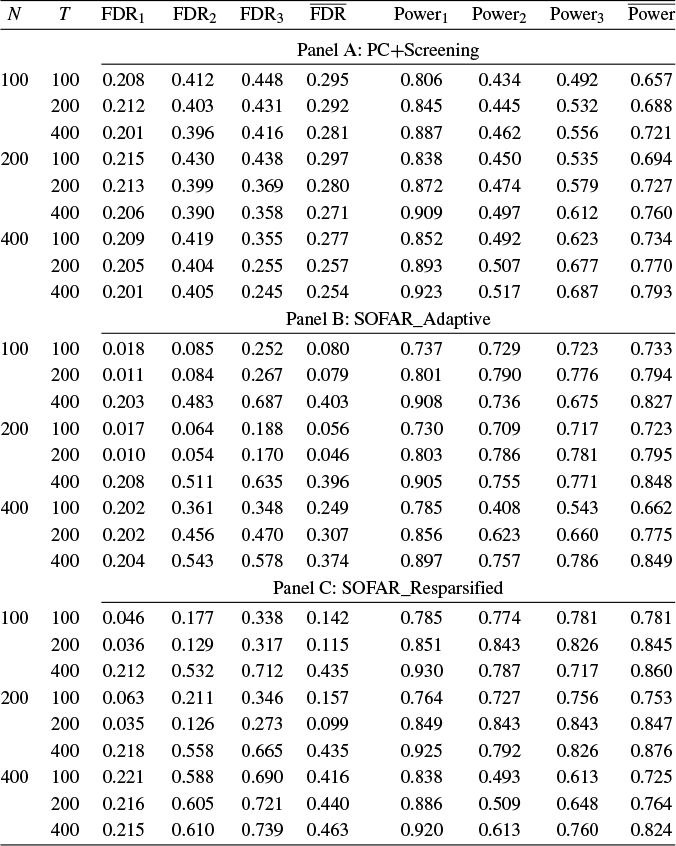
Table 2 shows that the results of FDR and power are better for stronger factors using either the PC or SOFAR-based method. Admittedly, the PC based method is inferior to SOFAR-based ones at relatively small or medium sample sizes. This is expected as the SOFAR-based methods explicitly target sparsity by additionally employing regularization or FDR control, while the simple PC estimators are inevitably subject to contamination distortion discussed in Section 4.1. Nevertheless, it is a bit surprising to see that FDR is abnormally high when either N or T is large for SOFAR, while it is decreasing with sample sizes for PC.Footnote
12
FDR and power under
 $r=3$

Moreover, in additional simulation, we try to work with very small gaps of factor strengths and present the FDR and power results for sparsity recovery in Table 11 in the Supplementary Material, which compares with Table 2 in the article with larger gaps of
 $\alpha =(0.9,0.75,0.6)$
. The results show that under the smaller gaps of strength, for factor 1, FDR is increasing from around 0.2 to around 0.3, although its power is quite robust; for factor 2, there is only mild deterioration for its FDR and power; the weakest factor 3 suffers most from the shrinking gaps. So perhaps we need to be cautious to work with a very weak factor whose strength is close to others.
We further investigate the estimated factor strength by various methods in Table 3. All estimates become less accurate as the true strength degree decreases, as expected. It is admitted that our proposed strength estimate (PC+Screening) suffers more of overestimation with fairly weak factors, e.g., those with
 $\alpha _{k}=0.6$
. This is likely attributed to the contamination discussed in Section 4.1, and also echoes the finding in Table 2. Otherwise, our estimate is comparable to, and sometimes even better than, those from SOFAR, which is designed deliberately for sparsity recovery, especially for strength
 $\alpha _{k} \in [0.7,0.9]$
. The message here again delivers the usefulness of our factor strength estimator, which works reasonably well while avoids involving heavy computation as in SOFAR. In addition, given the discussion in Remark 9, we also replace the screening value
 $c_{\lambda ,NT}$
with
 $\widetilde {c} _{\lambda ,NT}=c[\ln (N T)]^{-1 / 2}$
, and report the estimated factor strengths with
 $c=0.8$
and
 $1.2$
in Section F.2 of the Supplementary Material, which do not change much.
Estimation of factor strength when
 $r=3$
with
 $ \alpha =\left ( 0.9,0.75,0.6\right )$

6 CONCLUSION
This article analyzes the well-known approach of PCA, and derives several novel properties of it to deal with weak latent factor models with sparse factor loadings. It unveils an interesting and fundamental fact that the PC estimators can preserve the sparsity in estimated factor loadings for sparsity-induced weak factor models. This fact facilitates the derivation of asymptotic properties of PC estimators, enables us to recover the sparsity of loadings, and estimates the strengths of each factor. In addition, the determination of the number of factors in weak factor models is also investigated. The numerical studies confirm that our proposed approach works reasonably well in finite samples.
SUPPLEMENTARY MATERIAL
Jie Wei and Yonghui Zhang (2025): Supplement to “Can Principal Component Analysis Preserve the Sparsity in Factor Loadings?”, Econometric Theory Supplementary Material. To view, please visit: https://doi.org/10.1017/S0266466625100303.