3.1 Drag & deformation

Figure 2.

VoF function $\unicode[STIX]{x1D709}$ versus the normalized distance from the interface $y/h$ , showing the wall deformation for the different cases under investigation: (a) mean values and (b) root-mean-square (r.m.s.) of the fluctuations in $\unicode[STIX]{x1D709}$ . The blue, red, green and magenta solid lines are used for the cases $G1$ to $G4$ , respectively, while the particulate cases $G1_{10\,\%}$ to $G4_{10\,\%}$ are indicated with dashed lines of the same colour. The insets in (a) show the maximum and minimum position of the interface for different wall elasticities.

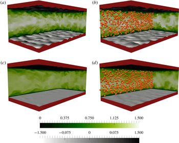
We first display snapshots of the flow and particles in figure 1, where the instantaneous streamwise velocity $u$ is depicted on $x$ – $y$ and $y$ – $z$ planes for the cases with $G^{\ast }=0.25$ and $1$ at $\unicode[STIX]{x1D719}=0$ and $10\,\%$ . For clarity, just a fraction of the particles (those cutting the visualized $x$ – $y$ plane) are displayed. Comparing with respect to the single-phase flow at the same wall elasticity (figure 1 a), particles are observed to decrease the wall deformation and turbulence activity in $G1_{10\,\%}$ (figure 1 b). However, the opposite effect is observed in $G3_{10\,\%}$ (figure 1 c,d), where the wall deformation is slightly increased in the presence of the particles. Also interesting to note is the spanwise coherency of the wall deformation in figure 1(a), which is broken into a less correlated pattern in the particulate case $G1_{10\,\%}$ (see figure 7 for a quantitative comparison).

To provide a quantitative measure of the wall deformation, the mean ( $\overline{\unicode[STIX]{x1D709}}$ ) and root-mean-square ( $\unicode[STIX]{x1D709}^{\prime }$ ) profiles of the VoF function $\unicode[STIX]{x1D709}$ representing the elastic walls are depicted in figure 2 versus the normalized distance from the interface $y/h$ . The maximum and minimum of the interface position, corresponding to the highest crests and the lowest troughs of the wavy interface, defined by the locations where $\overline{\unicode[STIX]{x1D709}}$ attains the values $0.999$ and $0.001$ , are reported in the insets of figure 2(a) for the different wall elasticities considered.

The results show an expected decrease of wall deformation with increasing $G^{\ast }$ for both single-phase and particulate cases. However, the effect of the particles on the wall deformation is non-monotonic: we find a slight decrease with respect to the single-phase flow in the cases with highly elastic walls ( $G1_{10\,\%}$ and $G2_{10\,\%}$ ), and a larger interface deformation for the cases with less wall elasticity in the presence of particles ( $G3_{10\,\%}$ and $G4_{10\,\%}$ ). Although the particles do not significantly change the maximum amplitude of the deformation, the approach of $\overline{\unicode[STIX]{x1D709}}$ to zero and one (insets of figure 2 a) is considerably modified: the data reveal the less frequent occurrence of large deformations in the particulate case at low $G^{\ast }$ and the opposite behaviour at high $G^{\ast }$ . The profiles of $\unicode[STIX]{x1D709}^{\prime }$ , depicted in figure 2(b), The peak value at $y=0$ indicates the degree of waviness at the interface. Given that $\overline{\unicode[STIX]{x1D709}}=0.5$ at the $y=0$ plane, the peak of $\unicode[STIX]{x1D709}^{\prime }$ is bounded between $\unicode[STIX]{x1D709}^{\prime }=0.5$ , where all the grid points in the $y=0$ plane are located inside the fluid region or in the elastic layer, and $\unicode[STIX]{x1D709}^{\prime }=0$ , where the interface is undeformed everywhere. The results show a decrease of the interface waviness by the presence of the particles in highly elastic walls, while the opposite is evident in the less deformable cases. This behaviour is attributed to the particle migration towards the centre of the channels with highly elastic walls and its resulting turbulence attenuation (see the next sections for the details).

Figure 3.

(a) Mean velocity profiles, normalized by the bulk velocity $U_{b}$ . The colour scheme is the same as figure 2 with two extra black lines, pertaining to the results for rigid walls (Ardekani et al. Reference Ardekani, Costa, Breugem, Picano and Brandt2017): a solid line for single-phase flow and a dashed line for particulate flow at $\unicode[STIX]{x1D719}=10\,\%$ . The inset displays the increase of the mean velocity in the core of the channel. (b) The friction Reynolds number $Re_{\unicode[STIX]{x1D70F}}$ versus the modulus of transverse elasticity $G^{\ast }$ . The black and red dashed horizontal lines in (b) represent $Re_{\unicode[STIX]{x1D70F}}$ for the single-phase and the particulate flow over smooth rigid walls.

The mean velocity profiles, obtained by averaging in the fluid phase, are presented in figure 3(a), together with two extra lines, pertaining to the results for rigid walls (Ardekani et al. Reference Ardekani, Costa, Breugem, Picano and Brandt2017). Note that the mean velocity inside the elastic walls is equal to zero. The results show that the mean velocity increases with the wall elasticity at the channel centreline for both particulate and single-phase cases, whereas it decreases close to the interface. Similarly to the flow over rigid walls (Picano et al. Reference Picano, Breugem and Brandt2015; Ardekani et al. Reference Ardekani, Costa, Breugem, Picano and Brandt2017), particles are observed to increase the core velocity, except for the cases with highly elastic walls ( $G1_{10\,\%}$ and $G2_{10\,\%}$ ), where the core velocity is reduced in their presence. We note here that unlike the single-phase flows over rigid walls, the mean velocity reduction close to the interface should not be interpreted as a sign of drag reduction. In fact, the friction Reynolds number $Re_{\unicode[STIX]{x1D70F}}$ , depicted in figure 3(b), indicates a significant drag increase with growing wall elasticity. Note that, $Re_{\unicode[STIX]{x1D70F}}$ is calculated using the mean pressure gradient needed to keep $U_{b}$ constant. Therefore, we find drag reduction with respect to the single-phase flow for same wall elasticity only for the particulate cases with highly elastic walls. Results concerning the case $G4_{NPWL}$ with artificially removed particle-wall layer and the cases with different volume fractions, $G2_{5\,\%}$ and $G2_{20\,\%}$ , will be discussed in § 3.3 and § 3.4. A comparison is made in appendix A between the results, pertaining to the single-phase flow and the case $G1_{FW}$ to distinguish the main effects of wall elasticity on the near-wall turbulence from the modulation caused by the roughness.

To better understand the overall drag, we perform a momentum budget analysis. In particulate turbulent flows with rigid walls, the particle-induced stress contributes to the mean momentum transfer, in addition to the viscous and Reynolds shear stresses. Here, we extend the formulation proposed by Zhang & Prosperetti (Reference Zhang and Prosperetti2010), Picano et al. (Reference Picano, Breugem and Brandt2015) for the momentum balance in particulate flows, by taking the hyper-elastic contribution into account (Rosti & Brandt Reference Rosti and Brandt2018). The mean momentum balance in the channel then reads

(3.1) $$\begin{eqnarray}\displaystyle \unicode[STIX]{x1D70C}u_{\unicode[STIX]{x1D70F}}^{2}\left(1-\frac{y}{h}\right)=\unicode[STIX]{x1D707}(1-\unicode[STIX]{x1D6F7})\frac{\text{d}U}{\text{d}y}-\unicode[STIX]{x1D70C}[\unicode[STIX]{x1D6F7}\langle u_{p}^{\prime }v_{p}^{\prime }\rangle +(1-\unicode[STIX]{x1D6F7})\langle u^{\prime }v^{\prime }\rangle ]+\langle \unicode[STIX]{x1D709}GB_{xy}\rangle +\unicode[STIX]{x1D6F7}\langle \unicode[STIX]{x1D70E}_{xy}^{p}\rangle ,\qquad & & \displaystyle\end{eqnarray}$$

where the first term on the right-hand side is the viscous shear stress, denoted $\unicode[STIX]{x1D70F}_{V}$ , the second and the third terms indicate the turbulent Reynolds shear stress of the combined phases, $\unicode[STIX]{x1D70F}_{T}$ , the fourth term is the contribution of the hyper-elastic wall, $\unicode[STIX]{x1D70F}_{E}$ and the fifth term is the particle-induced stress $\unicode[STIX]{x1D70F}_{P}$ ; $\unicode[STIX]{x1D70E}_{xy}^{p}$ in the equation above indicates the stress in the particle phase, normal to the streamwise plane and pointing in the wall-normal direction, $\unicode[STIX]{x1D6F7}$ is the mean local particle volume fraction as a function of the wall-normal distance and $u^{\prime }$ and $v^{\prime }$ are the velocity fluctuations in the streamwise and wall-normal directions with the subscript $_{p}$ denoting the particle phase. Here, $\unicode[STIX]{x1D70C}$ and $\unicode[STIX]{x1D707}$ are the density and viscosity, assumed equal in the fluid and the elastic layer. Note that in the absence of particles ( $\unicode[STIX]{x1D6F7}=0$ ) and the elastic layer ( $\unicode[STIX]{x1D709}=0$ ), this equation reduces to the classic momentum balance for single-phase turbulent channel flow (Pope Reference Pope2000).

The wall-normal profiles of each term in the momentum transfer, normalized by $\unicode[STIX]{x1D70C}u_{\unicode[STIX]{x1D70F}}^{2}$ , are displayed in figure 4(a–d) for the cases $G1$ , $G1_{10\,\%}$ , $G4$ and $G4_{10\,\%}$ . Note that the particle stress $\unicode[STIX]{x1D70F}_{P}$ is computed by subtracting the three other stresses from the total stress. Close to the interface, the contribution from the viscous stress $\unicode[STIX]{x1D70F}_{V}$ is reduced significantly with increasing wall elasticity, as the mean velocity is shown to decrease in this region (figure 3 a). The hyper-elastic stress, $\unicode[STIX]{x1D70F}_{E}$ , instead, takes over the momentum transfer, growing linearly within the elastic layer, where all other terms in equation (3.1) tend to zero. Note that, this line can be extrapolated to calculate the exact wall drag at $y=0$ , obtaining a drag which is consistent with the ones reported above based on the mean pressure gradient. Far from the interface region, the Reynolds stress, $\unicode[STIX]{x1D70F}_{T}$ , plays the main role in momentum transfer. The relative importance of the particle stress $\unicode[STIX]{x1D70F}_{P}$ is observed to increase with the wall elasticity, while the peak close to the interface disappears.

Figure 4.

Momentum budget, normalized with $\unicode[STIX]{x1D70C}u_{\unicode[STIX]{x1D70F}}^{2}$ , for (a)  $G1$ , (b)  $G1_{10\,\%}$ , (c)  $G4$ and (d)  $G4_{10\,\%}$ . Here, $\unicode[STIX]{x1D70F}$ is the total stress, $\unicode[STIX]{x1D70F}_{V}$ the viscous shear stress, $\unicode[STIX]{x1D70F}_{T}$ the turbulent Reynolds shear stress of the combined phases, $\unicode[STIX]{x1D70F}_{E}$ the hyper-elastic contribution and $\unicode[STIX]{x1D70F}_{P}$ the particle induced stress. Panels (e) and (f) show the total contribution of each stress to the drag, normalized by the wall shear stress of the single-phase flow with rigid walls, $\unicode[STIX]{x1D70F}_{RW}$ (the dashed line in the figure). $RW$ and $RW_{10\,\%}$ are the cases with rigid walls taken by Ardekani et al. (Reference Ardekani, Costa, Breugem, Picano and Brandt2017).

Integrating equation (3.1) from $0$ to $h$ leads to the contribution of each stress to the total $\unicode[STIX]{x1D70F}_{w}$ , which can be written as

(3.2) $$\begin{eqnarray}\displaystyle \unicode[STIX]{x1D70F}_{w}=\frac{2}{h}[\unicode[STIX]{x1D6F4}\unicode[STIX]{x1D70F}_{V}+\unicode[STIX]{x1D6F4}\unicode[STIX]{x1D70F}_{T}+\unicode[STIX]{x1D6F4}\unicode[STIX]{x1D70F}_{E}+\unicode[STIX]{x1D6F4}\unicode[STIX]{x1D70F}_{P}]. & & \displaystyle\end{eqnarray}$$

Each contribution, multiplied by $2/h$ and normalized with the wall shear stress of the single-phase flow over rigid walls ( $\unicode[STIX]{x1D70F}_{RW}$ ), is reported in figure 4(e,f) for the single-phase and the particulate cases with different wall elasticities; $RW$ and $RW_{10\,\%}$ are obtained from the simulations with rigid walls presented in Ardekani et al. (Reference Ardekani, Costa, Breugem, Picano and Brandt2017). Overall, we observe that the increase in drag with wall deformability can be attributed to an increase of the turbulence activity, as also discussed in Rosti & Brandt (Reference Rosti and Brandt2017). In other words, the turbulence activity increases with respect to the reference $RW$ for all cases. The contribution of the viscous shear stress to the total drag is in general reduced with increasing wall elasticity, whereas the particle stress $\unicode[STIX]{x1D6F4}\unicode[STIX]{x1D70F}_{P}$ monotonically increases with decreasing $G^{\ast }$ . This can be explained by the rigid particles opposing any deformation, while experiencing stronger forces on their surfaces due to the growing turbulence activity with decreasing $G^{\ast }$ . We also note a non-monotonic variation of $\unicode[STIX]{x1D6F4}\unicode[STIX]{x1D70F}_{T}$ and $\unicode[STIX]{x1D6F4}\unicode[STIX]{x1D70F}_{E}$ in the particle-laden cases when comparing the results with the single-phase flows of the same wall elasticity: turbulence attenuation for highly elastic walls, while increasing the turbulence activity in the cases of less deformable walls.

3.2 Turbulence modulation

Figure 5.

Root-mean-square velocity fluctuations and Reynolds shear stress: (a) streamwise $\langle |u^{\prime }|\rangle$ ; (b) wall normal $\langle |v^{\prime }|\rangle$ ; (c) spanwise $\langle |w^{\prime }|\rangle$ and (d) Reynolds shear stress. Panels (e) and (f) show $\langle |u^{\prime }|\rangle$ and $\langle |v^{\prime }|\rangle$ , scaled in internal units. The colour scheme is the same as in figures 2 and 3(a).

In this section we take a closer look at the turbulence modulation caused by the simultaneous presence of the particles and deformable walls. We first examine the root-mean-square velocity fluctuations and the Reynolds shear stress profiles, depicted in figure 5. The velocity fluctuations are strongly affected by the elastic layer, lingering inside as the wall elasticity increases. The wall-normal velocity fluctuation $v^{\prime }$ is the most affected by the wall elasticity, owing to the weakening of the wall blocking and wall-induced viscous effects (Perot & Moin Reference Perot and Moin1995a ,Reference Perot and Moin b ). The same effect is also observed in turbulent boundary-layer flows over rough (Krogstadt & Antonia Reference Krogstadt and Antonia1999) and porous walls (Rosti, Brandt & Pinelli Reference Rosti, Brandt and Pinelli2018b ). In addition, we note that $\langle |v^{\prime }|\rangle$ attains a secondary peak in the vicinity of the interface, associated with the oscillatory interface motion. As the wall elasticity increases, this secondary peak moves farther from the interface, becomes stronger than the classical turbulent peak and the fluctuations are larger at the interface. In addition, we note that the peak of the streamwise velocity fluctuations, $u^{\prime }$ , increases with increasing wall elasticity considerably less than in the other two directions, which we attribute to the quenching of the near-wall streaky structures close to the deformable interface (Breugem et al. Reference Breugem, Boersma and Uittenbogaard2006; Rosti & Brandt Reference Rosti and Brandt2017; Rosti et al. Reference Rosti, Brandt and Pinelli2018b ). This behaviour is particularly evident in figure 5(e,f), where the profiles of $\langle |u^{\prime }|\rangle$ and $\langle |v^{\prime }|\rangle$ are depicted in internal units.

The magnitude of the velocity fluctuations increases in the presence of particles for low wall deformabilities while it decreases for high elasticity, except for the peaks of $\langle |u^{\prime }|\rangle$ which are always reduced with respect to their single-phase counterparts. Despite the strong velocity fluctuations also inside the highly elastic walls, the Reynolds shear stress (see figure 5 d) is zero within these layers, indicating a decorrelation of $u^{\prime }$ and $v^{\prime }$ . The Reynolds shear stress increases in the particulate cases, except in the presence of highly elastic walls, as observed for the r.m.s. velocities, where a significant attenuation is instead observed (also shown in figure 4 f).

Figure 6.

Instantaneous contours of the streamwise velocity fluctuations $u^{\prime }$ in the wall-parallel plane $x-z$ at $y/h=0.1$ . The colour scale goes from $-0.5U_{b}$ (blue) to $0.5U_{b}$ (yellow). (a,c,e,g) indicates the single-phase flow cases ( $G1$ to $G4$ ) and (b,d,f,h), the particulate ones ( $G1_{10\,\%}$ to $G4_{10\,\%}$ ), with $G^{\ast }$ increasing from (a–h).

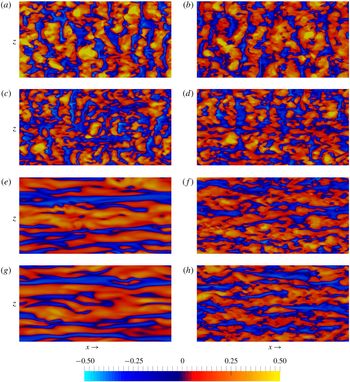
Next, we take a closer look at the turbulent flow near the deformable walls, see figure 6 where we report instantaneous snapshots of the streamwise velocity fluctuations, $u^{\prime }$ , in the wall-parallel plane at $y/h=0.1$ . The so-called high- and low-speed streaks, characteristic of wall-bounded turbulence, can be directly recognized near the less elastic walls. As the wall elasticity increases (from bottom to top), these streamwise streaky structures appear as less elongated and more fragmented, broken into smaller pieces by the interface motion. Further increasing the wall elasticity results in the formation of relatively large structures, now correlated in the spanwise direction (a), similar to those observed by Rosti & Brandt (Reference Rosti and Brandt2017). These spanwise structures have been observed before in the turbulent flow over porous walls (Breugem et al. Reference Breugem, Boersma and Uittenbogaard2006; Rosti et al. Reference Rosti, Cortelezzi and Quadrio2015, Reference Rosti, Brandt and Pinelli2018b ), rough surfaces (Raupach, Antonia & Rajagopalan Reference Raupach, Antonia and Rajagopalan1991; Jiménez et al. Reference Jiménez, Uhlmann, Pinelli and Kawahara2001) and plant canopies (Finnigan Reference Finnigan2000). Breugem et al. (Reference Breugem, Boersma and Uittenbogaard2006) relates these elongated structures to a Kelvin–Helmholtz-type instability that is triggered by the inflection point of the mean velocity profiles (Rayleigh’s criterion, see Drazin & Reid Reference Drazin and Reid2004), creating spanwise vortices or rollers. Snapshots of $u^{\prime }$ in the flow laden with particles are shown in figure 6(b,d,f,h). Particles can be observed to break both the streamwise and the spanwise structures into less elongated and more fragmented patches.

Figure 7.

Line and colour contours of the one-dimensional autocorrelation of (a) the streamwise velocity fluctuations as a function of the spanwise spacing ( $R_{uu}^{z}(y,\unicode[STIX]{x0394}z)$ ) and (b) the wall-normal velocity fluctuations as a function of the streamwise spacing for different $y/h$ ( $R_{vv}^{x}(y,\unicode[STIX]{x0394}x)$ ). The solid lines correspond to positive values, ranging from $0$ to $0.8$ with a step of $0.2$ between two neighbouring lines, whereas dashed and dotted lines indicate the isolines at $-0.1$ and $-0.2$ , respectively. Results, pertaining to the single-phase flow (cases $G1$ to $G4$ ), are shown in the first row of each panel, while the autocorrelations for the particulate cases (cases $G1_{10\,\%}$ to $G4_{10\,\%}$ ) are depicted in the second row. $G^{\ast }$ increases from left to right. Internal units are indicated on the top and on the right side of each panel.

To gain a better understanding of the turbulence structures and in order to quantify the observations in figure 6, we compute the two-point spatial correlation of the streamwise and the wall-normal velocity fluctuations as a function of the spanwise and streamwise spacing, respectively as

(3.3) $$\begin{eqnarray}\displaystyle & \displaystyle R_{uu}^{z}(y,\unicode[STIX]{x0394}z)=\frac{\langle u^{\prime }(x,y,z,t)u^{\prime }(x,y,z+\unicode[STIX]{x0394}z,t)\rangle }{{u^{\prime }}^{2}}, & \displaystyle\end{eqnarray}$$

(3.4) $$\begin{eqnarray}\displaystyle & \displaystyle R_{vv}^{x}(y,\unicode[STIX]{x0394}x)=\frac{\langle v^{\prime }(x,y,z,t)v^{\prime }(x+\unicode[STIX]{x0394}x,y,z,t)\rangle }{{v^{\prime }}^{2}}. & \displaystyle\end{eqnarray}$$

Line and colour contours of $R_{uu}^{z}(y,\unicode[STIX]{x0394}z)$ and $R_{vv}^{x}(y,\unicode[STIX]{x0394}x)$ are presented in figure 7(a,b) for the different cases under investigation. It is known that in a single-phase turbulent flow the spanwise correlation of the streamwise velocity fluctuations exhibits a negative local minimum in the near-wall region at around $\unicode[STIX]{x0394}z^{+}\approx 50{-}60$ (Pope Reference Pope2000), which indicates half of the spacing between two neighbouring streaks. A similar spacing is obtained in figure 7(a) for the cases with less elastic walls $G3$ and $G4$ (top right), as these display a local minimum at $\unicode[STIX]{x0394}Z^{+}\approx 55$ and $\unicode[STIX]{x0394}Z^{+}\approx 58$ , respectively. The figure shows clearly the disruption of the high- and low-speed streaks, when increasing the wall elasticity, and how they shift away from the interface region. The absence of high- and low-speed streaks, close to the highly elastic walls, can be attributed to (i) a strong reduction of the mean shear (see figure 3 a), an important ingredient in the streaks formation mechanism (Lee, Kim & Moin Reference Lee, Kim and Moin1990; Brandt Reference Brandt2014) and (ii) strong wall-normal velocity fluctuations preventing the development of elongated structures. A region of positive values of $R_{uu}^{z}$ can be observed instead, at $y/h\approx 0.1$ and $0.07$ for the highly elastic cases, $G1$ and $G2$ : this indicates the emergence of structures elongated in the spanwise direction (as expected from the visualizations in figure 6) with an approximate length of $0.7{-}0.8h$ .

The correlation $R_{uu}^{z}$ pertaining to the particulate cases is given in the second row of figure 7(a). The addition of particles shortens the spanwise length of the structures in the cases $G1_{10\,\%}$ and $G2_{10\,\%}$ ; the wall elasticity disrupts and displaces the high- and low-speed streaks towards the channel centre. The disruption of the near-wall streaks has been reported before for turbulent channel flows of finite-size spherical particles (Picano et al. Reference Picano, Breugem and Brandt2015; Costa et al. Reference Costa, Picano, Brandt and Breugem2018; Wang, Abbas & Climent Reference Wang, Abbas and Climent2018; Ardekani & Brandt Reference Ardekani and Brandt2019).

Next, we show the autocorrelations of the wall-normal velocity fluctuations along the streamwise direction $R_{vv}^{x}(y,\unicode[STIX]{x0394}x)$ , see figure 7(b). The results clearly reveal that the long quasi-streamwise vortices, associated with the presence of streaks, vanish when increasing the wall elasticity and are replaced by roller-type vortices, elongated in the spanwise direction. The active range of these vortical structures grows with the wall elasticity, reaching a size of approximately $140^{+}$ in the most elastic case $G1$ . In the particle-laden flows, the height of these vortices reduces in the highly elastic cases, whereas the quasi-streamwise vortices characteristic of the less deformable cases become shorter and more irregular. Breaking the large spanwise vortices near highly elastic walls results in less wall deformation and thus, an overall attenuation of the turbulent activity (see also figure 1 b); however, it should be also noted that breaking the quasi-streamwise vortices does not necessarily decrease the turbulent activity. Indeed, it has been shown before that spherical particles with the same size and volume fraction as considered here induce an increase of the turbulent activity near rigid walls (Picano et al. Reference Picano, Breugem and Brandt2015; Ardekani et al. Reference Ardekani, Costa, Breugem, Picano and Brandt2017), similarly to what observed in this study for the less elastic cases (see figure 5 d).

Figure 8.

Contours of the weighted Reynolds shear stress at $y/h=0.05$ , given by multiplying the absolute value of the Reynolds shear stress by the joint probability density of its occurrence in the $u^{\prime }{-}v^{\prime }$ plane for: (a) the single-phase flow cases $G1$ to $G4$ , (b) the particulate cases $G1_{10\,\%}$ to $G4_{10\,\%}$ and (c) spherical shells 5 % larger than the particles in $G1_{10\,\%}$ to $G4_{10\,\%}$ . $G^{\ast }$ increases from left to right and the colours go from yellow to black (maximum).

So far we have presented a picture of the turbulence coherent structures near elastic walls, including the presence of finite-size particles; however, the way these structures contribute to the enhancement or attenuation of the Reynolds shear stress is yet to be understood. To this purpose, we compute the weighted Reynolds shear stress, obtained by multiplying the absolute value of Reynolds shear stress with the joint probability density of its occurrence in the $u^{\prime }{-}v^{\prime }$ plane (Zhou et al. Reference Zhou, Adrian, Balachandar and Kendall1999). This analysis indicates the turbulent events that contribute the most to the Reynolds shear stress, dividing them into the four quadrants of the $u^{\prime }{-}v^{\prime }$ plane, denoted $Q_{1}$ to $Q_{4}$ . In particular, $Q_{2}$ (ejections: $u^{\prime }<0$ , $v^{\prime }>0$ ) and $Q_{4}$ (sweeps: $u^{\prime }>0$ , $v^{\prime }<0$ ) events result in turbulence production, while $Q_{1}$ and $Q_{3}$ are responsible for damping.

Contours of the weighted Reynolds shear stress are depicted in figure 8 for a wall-parallel plane slightly above the elastic wall $y/h=0.05$ ; $y/h=0.05$ approximately matches the particle radius and is chosen to indicate the effect of the particles close to the wall on the near-wall turbulence. Panel (a) shows the results for the single-phase cases with elasticity decreasing from left to right. The major contribution to the turbulence production near the highly elastic walls comes from ejection events with significantly large values of $v^{\prime }$ and small negative $u^{\prime }$ ; the contribution of sweeps comes from the events with an opposite combination, i.e. small negative $v^{\prime }$ and a relatively large positive $u^{\prime }$ . This observation reveals the mechanism by which the spanwise vortices, forming close to the highly elastic walls, contribute to the turbulence production: these vortices bring down the high momentum flow towards the elastic wall with a weak wall-normal velocity due to the decreased wall-blocking effect of the elastic layer, thus deforming the interface. The interface then releases this elastic energy by pushing the flow with a strong wall-normal velocity towards the centre of the channel, contributing to the turbulence production and regeneration of new spanwise vortical structures. The low magnitude of $u^{\prime }$ in the ejection events is believed to be due to the blocking effect from the upstream deformed interface. This is consistent with the asymmetric shape of the deformed wall (steeper slope for wall retraction), previously shown in figure 1(a). As the wall elasticity decreases, the distribution of the strong ejection events over the $u^{\prime }{-}v^{\prime }$ plane appears to become less elongated in the vertical direction ( $v^{\prime }$ axis), while stretching along the $u^{\prime }$ axis. The relative contribution of sweep events increases when lowering the wall elasticity, although with smaller magnitudes of $u^{\prime }v^{\prime }$ . The distribution for the least elastic case (b) is similar to what found in turbulent flows in the vicinity of rigid walls (Kim et al. Reference Kim, Moin and Moser1987), where the sweep events are slightly more powerful than the ejections.

The results pertaining to the particulate cases are depicted in figure 8(b). The shapes of the distribution are similar to the ones of the single-phase flow cases, except for an increase ( $G3_{10\,\%}$ and $G4_{10\,\%}$ ) or a reduction ( $G1_{10\,\%}$ and $G2_{10\,\%}$ ) in the magnitude of $v^{\prime }$ . To gain a better understanding of the particles role, we repeat the same analysis in figure 8(c), now sampling only the fluid inside a spherical shell which is $5\,\%$ larger than the particles (particles cutting the wall-normal plane $y/h=0.05$ ). For the cases with highly elastic walls, the particles approach the interface region and are trapped inside strong sweep events with a relatively large streamwise velocity. The asymmetry in the magnitude of the wall-normal fluctuations (larger magnitudes for positive $v^{\prime }$ ) causes the particles to move away from the wall considerably faster than when approaching it. Therefore, it is more likely to sample particles which are slowly approaching the wall, surrounded by $Q_{4}$ events. It should be noted here that the particle concentration is low in the vicinity of highly elastic walls as we will discuss later in § 3.3 and thus, the strong sweep events around the particles do not contribute significantly to the turbulent production. Indeed, particles reduce the active range of the large spanwise vortices, causing smaller wall deformation and in turn a turbulence attenuation. In addition to sweeps, stronger $Q_{1}$ events appear in the flow surrounding the particles when the wall elasticity decreases. This is due to particles with large streamwise velocity bouncing back from the less deformable walls. Even though $Q_{1}$ events damp the turbulence activity, the increase in the wall-normal velocity fluctuations and also stronger sweeps close to the wall result in an overall enhancement of the turbulent activity. The same conclusion can be drawn from figure 9, where the Reynolds shear stress is conditionally averaged and depicted for the second ( $Q_{2}$ ) and the fourth ( $Q_{4}$ ) quadrants of the $u^{\prime }{-}v^{\prime }$ plane against $y/h$ . Interestingly, both ejection and sweep events are damped in the presence of the particles for the highly elastic walls; while for the less elastic cases, turbulence is enhanced through sweep events and ejections are almost unchanged with respect to the single-phase cases.

Figure 9.

Reynolds shear stress, conditionally averaged for (a) the second ( $Q_{2}$ ) and (b) the fourth ( $Q_{4}$ ) quadrant of $u^{\prime }{-}v^{\prime }$ plane.

3.3 Particle dynamics

The mean local volume fraction $\unicode[STIX]{x1D6F7}$ is depicted in figure 10(a). Spherical particles in the turbulent flow with rigid walls (case $RW_{10\,\%}$ ) display a local maximum at a distance slightly larger than one particle radius from the wall. Picano et al. (Reference Picano, Breugem and Brandt2015) attributed this local maximum to the formation of a particle layer at the wall due to the wall–particle interactions that stabilize the particle position. Costa et al. (Reference Costa, Picano, Brandt and Breugem2016) further explained that the presence of this particle layer always results in drag increase with respect to the single-phase flow. Interestingly, the local maximum for $\unicode[STIX]{x1D6F7}$ is observed to reduce and move farther away from the wall when increasing the wall elasticity. The migration of the particles from the interface region can be explained by the presence of the strong ejection events with large $v^{\prime }$ in the flow in the case of highly elastic walls (see figure 8). Indeed, the strong asymmetry in the magnitude of the wall-normal velocity fluctuations, which favours positive $v^{\prime }$ , pushes the inertial particles towards the channel centre. However, as the wall elasticity decreases, a more symmetric distribution of $v^{\prime }$ allows the particles to form a layer close to the interface, similarly to the rigid wall cases. This particle-wall layer contributes to the turbulent production by increasing the cross-flow velocity fluctuations, as shown in the previous subsection.

To study the particle dynamics, we display in figure 10(b) the ratio between the turbulent kinetic energy of the fluid and that of the particle phase, $K_{f}^{\prime }/K_{p}^{\prime }=\langle {u^{\prime }}^{2}+{v^{\prime }}^{2}+{w^{\prime }}^{2}\rangle /\langle {u_{p}^{\prime }}^{2}+{v_{p}^{\prime }}^{2}+{w_{p}^{\prime }}^{2}\rangle$ . For the particle statistics presented in this figure the rigid body motion of the particles is taken into account. The local velocity of the particle phase is computed at each point by $\boldsymbol{u}_{p}+\pmb{\unicode[STIX]{x1D6FA}}_{p}\times (\boldsymbol{x}-\boldsymbol{x}_{c})$ , with $\boldsymbol{x}$ and $\boldsymbol{x}_{c}$ denoting an arbitrary point inside the particle and the particle centre, respectively. Particle velocities are observed to fluctuate less than the fluid at the same wall-normal distance, except for a tiny region close to the wall ( $y/h\lessapprox 0.05$ ), where the ratio is below $1$ for all the cases. The high particle fluctuation level in this region suggests that this is the cause of the near-wall enhancement of the fluid velocity fluctuations, observed in the cases with less elastic walls. The ratio between the two energies increases with the wall elasticity at $y=0$ , reaching $0.6$ in the most elastic case, when fewer particles can be found in this region. Particle–wall/particle collisions are observed to play an important role in increasing the fluctuations near the wall. Indeed, the particles in this region have a mean velocity larger than the surrounding fluid, due to their size and the fact that they can have a relative tangential motion at the wall. Therefore, any collision between the particles can result in strong velocity fluctuations. Figure 10(c) depicts the mean particle velocity profiles, normalized by the bulk velocity $U_{b}$ . Comparing the profiles with the mean velocity in figure 3(a) reveals that the particle and fluid phase have the same mean velocity throughout the channel, except for a small layer close to the wall with the width of approximately one particle diameter $D$ , where particles experience a larger mean velocity. The slip velocity at $y=0$ is observed to increase as the wall elasticity decreases.

Figure 10.

Profiles of particle-phase averaged data versus $y/h$ : (a) mean local volume fraction, (b) the ratio between the turbulent kinetic energy of the fluid and of the particle phase and (c) mean particle velocity profiles, normalized by the bulk velocity $U_{b}$ . $RW_{10\,\%}$ refers to the case with rigid walls from the study of Ardekani et al. (Reference Ardekani, Costa, Breugem, Picano and Brandt2017). (d) Overall average particle velocity versus the modulus of transverse elasticity $G^{\ast }$ . The average of the particle velocity for $RW_{10\,\%}$ is indicated with a dotted line.

The overall average particle velocity is displayed in figure 10(d) versus the modulus of transverse elasticity $G^{\ast }$ . It can be observed in this figure that increasing the wall elasticity results in a faster transport of the solid phase as the averaged velocity increases from approximately $1.06U_{b}$ in the case of rigid walls (shown with a dotted horizontal line) to $1.14$ in the flow over the most elastic walls. This increase in the averaged velocity is due to the migration of the particles away from the interface region.

Figure 11.

(a) Root-mean-square velocity fluctuations $u^{\prime }$ , $v^{\prime }$ and $w^{\prime }$ in the streamwise, ——, wall-normal, - - -  and spanwise, …, directions and (b) Reynolds shear stress, scaled in outer units for the cases $G4$ , $G4_{10\,\%}$ and $G4_{NPWL}$ .

To show the importance of the particle-wall layer in the enhancement of the velocity fluctuations in this region, we perform a numerical experiment where we artificially remove this layer. In this simulation, denoted $G4_{NPWL}$ (no particle-wall layer), particles bounce back towards the core region of the channel before approaching the elastic walls, colliding with two virtual walls located at a distance $h/10$ from the two real interfaces ( $y/h=0.1$ ). 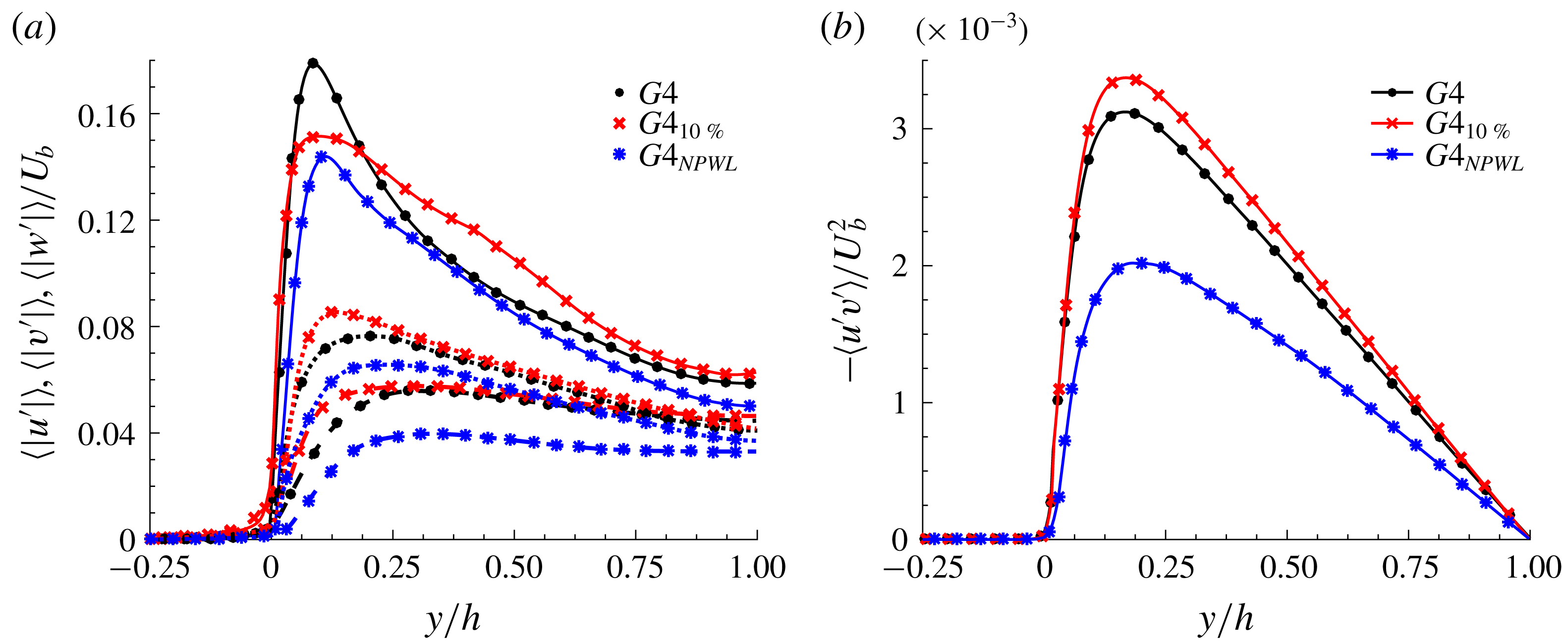The elasticity of the wall is set to $G^{\ast }=2$ , i.e. the less deformable elastic wall previously considered, the case where the effect of the particle-wall layer is more pronounced. The velocity fluctuations and the Reynolds shear stress pertaining to this additional case are compared with the results for $G4$ and $G4_{10\,\%}$ in figure 11. The increase in the cross-flow fluctuations previously observed for the case $G4_{10\,\%}$ disappears when removing the particle-wall layer ( $G4_{NPWL}$ ), and as a consequence, a strong turbulence attenuation is obtained (see figure 11 b), with $v^{\prime }$ the most reduced fluctuation component. With particles not contributing to the turbulent production in the near-wall region, the attenuation of the turbulence activity can be associated with the increased effective viscosity of the suspension (Picano et al. Reference Picano, Breugem and Brandt2015; Ardekani et al. Reference Ardekani, Costa, Breugem, Picano and Brandt2017). The effective viscosity of a rigid particle suspension is always higher than that of the single-phase flow, which cause a reduction in the turbulent activity; however, this effect is usually compensated by the formation of a particle-wall layer and its contribution to the turbulence production, thus resulting in an overall enhancement of the turbulent activity ( $G4$ ). Hence, a strong turbulence attenuation and thus drag reduction ( $Re_{\unicode[STIX]{x1D70F}}\approx 167$ ) even with respect to the single-phase flow over rigid walls ( $Re_{\unicode[STIX]{x1D70F}}\approx 180$ ) can be obtained by removing the particle-wall layer (see figure 3 b).

3.4 Effect of the particle volume fraction

Figure 12.

Instantaneous snapshots of the streamwise velocity $u$ on the $x$ – $y$ and $y$ – $z$ planes for walls with elastic modulus $G^{\ast }=0.5$ and different volume fractions (a)  $\unicode[STIX]{x1D719}=0\,\%$ (case $G2$ ), (b)  $\unicode[STIX]{x1D719}=5\,\%$ (case $G2_{5\,\%}$ ), (c)  $\unicode[STIX]{x1D719}=10\,\%$ (case $G2_{10\,\%}$ ) and (d)  $\unicode[STIX]{x1D719}=20\,\%$ (case $G2_{20\,\%}$ ). For clarity, only the particles lying within the selected $x$ – $y$ plane are displayed. The colour scale for the streamwise velocity ranges from $0$ (dark green) to $1.5u/U_{b}$ (white). The elastic walls are represented by the isosurface $\unicode[STIX]{x1D709}=0.5$ , coloured by the wall-normal distance, ranging from $-0.15h$ (white) to $0.15h$ (black).

Picano et al. (Reference Picano, Breugem and Brandt2015) investigated dense suspensions of spherical particles in a turbulent channel flow with rigid walls up to a volume fraction equal to $20\,\%$ . Their study revealed that the overall drag increase is mainly due to the enhancement of the turbulence activity up to $\unicode[STIX]{x1D719}=10\,\%$ and to the particle-induced stress at higher concentrations ( $\unicode[STIX]{x1D719}=20\,\%$ ), where the turbulence is instead attenuated. In this section we investigate the effect of the particle volume fraction in a channel with elastic walls. The case $G2$ , with elasticity $G^{\ast }=0.5$ , is simulated with two additional volume fractions, $\unicode[STIX]{x1D719}=5\,\%$ and $20\,\%$ , so to compare the change in drag with respect to the cases with rigid walls.

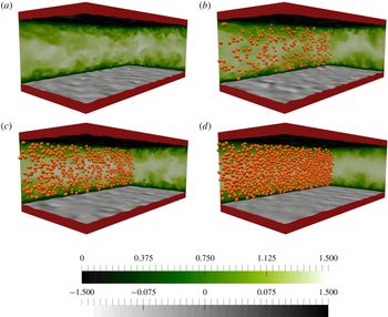
Snapshots of the flow and particles are displayed in figure 12, where the instantaneous streamwise velocity $u$ is depicted on $x$ – $y$ and $y$ – $z$ planes for the cases with $G^{\ast }=0.5$ and $\unicode[STIX]{x1D719}=0$ , $5\,\%$ , $10\,\%$ and $20\,\%$ . For clarity, just a fraction of the particles (those lying within the visualized $x$ – $y$ plane) are displayed. The wall deformation and the turbulent activity appear to decrease when increasing the particle volume fraction, especially in the case with $\unicode[STIX]{x1D719}=20\,\%$ . Note also the absence of a particle-wall layer close to the interface, even at highest volume fraction considered here, $\unicode[STIX]{x1D719}=20\,\%$ .

Figure 13.

(a) Root-mean-square velocity fluctuations $u^{\prime }$ , $v^{\prime }$ and $w^{\prime }$ in the streamwise, ——, wall-normal, - - -, and spanwise, …, directions. (b) Mean local volume fraction profiles against the results for rigid walls (Picano et al. Reference Picano, Breugem and Brandt2015). (c) The total contribution of each stress to the drag at the interface, normalized by the drag of the single-phase flow with rigid walls, $\unicode[STIX]{x1D70F}_{RW}$ (the dashed line with $Re_{\unicode[STIX]{x1D70F}}=180$ ). The case $RW_{20\,\%}$ (rigid walls at $\unicode[STIX]{x1D719}=20\,\%$ ) is extracted from the reported data in Picano et al. (Reference Picano, Breugem and Brandt2015). (d) The friction Reynolds number $Re_{\unicode[STIX]{x1D70F}}$ , versus the volume fraction $\unicode[STIX]{x1D719}$ .

The root-mean-square velocity fluctuations $\langle |u^{\prime }|\rangle$ , $\langle |v^{\prime }|\rangle$ and $\langle |w^{\prime }|\rangle$ are depicted in figure 13(a), versus the wall-normal distance $y/h$ . The results show a progressive reduction in the velocity fluctuations with increasing solid volume fraction. The decrease with respect to $G2$ is moderate for $G2_{5\,\%}$ and $G2_{10\,\%}$ , while for a volume fraction of $20\,\%$ a significant attenuation of all the velocity fluctuations is evident, especially in the core of the channel where the turbulent flow is almost relaminarized (see also figure 12 d). Differently from the results with rigid walls (Picano et al. Reference Picano, Breugem and Brandt2015), the particles are observed here to attenuate the turbulence activity for all the volume fractions, with a reduction larger than that with rigid walls for the case at $\unicode[STIX]{x1D719}=20\,\%$ . We explain this by examining the mean local volume fraction profiles in figure 13(b), where data for rigid walls are also displayed (Picano et al. Reference Picano, Breugem and Brandt2015). The particle-wall layer disappears for $\unicode[STIX]{x1D719}\leqslant 10\,\%$ and the near-wall peak is significantly reduced and displaced farther away from the wall ( $y/h\approx 0.1$ ) also for the case $G2_{20\,\%}$ . The particle migration away from the interface region causes a stronger attenuation of turbulence than in the presence of rigid walls at $\unicode[STIX]{x1D719}=20\,\%$ .

Following the analysis in equation (3.2), the contribution of each shear stress (viscous, $\unicode[STIX]{x1D70F}_{V}$ , Reynolds, $\unicode[STIX]{x1D70F}_{T}$ , hyper-elastic, $\unicode[STIX]{x1D70F}_{E}$ and particle-induced $\unicode[STIX]{x1D70F}_{P}$ ), normalized by the drag of the single-phase flow over rigid walls ( $\unicode[STIX]{x1D70F}_{RW}$ ), is reported in figure 13(c) for different volume fractions at $G^{\ast }=0.5$ . The case $RW_{20\,\%}$ denotes the flow at $\unicode[STIX]{x1D719}=20\,\%$ over rigid walls from Picano et al. (Reference Picano, Breugem and Brandt2015). In spite of a reduced turbulent activity over an elastic wall, case $G2_{20\,\%}$ in comparison to $RW_{20\,\%}$ , the particle stress $\unicode[STIX]{x1D70F}_{P}$ more than compensates for the decrease of Reynolds shear stress, resulting in an overall higher drag for the flow over the elastic wall. The friction Reynolds number, $Re_{\unicode[STIX]{x1D70F}}$ , is finally compared with the results for rigid walls in figure 13(d), where the effect of wall elasticity is observed to reduce significantly when the volume fraction of the particles is increased.