2 Computation of spatial optimal disturbances

The optimization scheme developed in this work is based on the computation of the spatial evolution of small disturbances using the parabolized stability equations (Bertolotti, Herbert & Spalart Reference Bertolotti, Herbert and Spalart1992; Herbert Reference Herbert1997). The PSE are derived from the incompressible linearized Navier–Stokes equations,

which describe the evolution of small perturbations, $\boldsymbol{q}=(\boldsymbol{u}^{\text{T}},p)^{\text{T}}=(u,v,w,p)^{\text{T}}$ to the base flow $\boldsymbol{U}=(U,V,W)^{\text{T}}$ . The ansatz

is invoked, where $\hat{\boldsymbol{q}}$ is the complex disturbance shape function, $\unicode[STIX]{x1D6FC}$ is a complex streamwise wavenumber, $\unicode[STIX]{x1D6FD}$ is a real spanwise wavenumber and $\unicode[STIX]{x1D714}$ is a real temporal frequency. The ambiguity arising from the dependence of both $\hat{\boldsymbol{q}}$ and $\unicode[STIX]{x1D6FC}$ on $x$ is resolved by requiring that

where superscript $\unicode[STIX]{x1D643}$ denotes the conjugate transpose. The shape function $\hat{\boldsymbol{q}}(x,y)$ hence only weakly depends on the streamwise coordinate. Retaining terms up to order $O(Re^{-1})$ , the governing equations take the form,

The definitions of the matrices $\unicode[STIX]{x1D63C}$ , $\unicode[STIX]{x1D63D}$ , $\unicode[STIX]{x1D63E}$ and $\unicode[STIX]{x1D63F}$ for a general, three-dimensional base state $\boldsymbol{U}(x,y)=(U,V,W)^{\text{T}}$ are

with $r=-\text{i}\unicode[STIX]{x1D714}+\text{i}\unicode[STIX]{x1D6FC}U+\text{i}\unicode[STIX]{x1D6FD}W+(\unicode[STIX]{x1D6FC}^{2}+\unicode[STIX]{x1D6FD}^{2})/Re$ . In this formulation, the spatial marching scheme of the PSE has been regularized by disregarding the term $\unicode[STIX]{x2202}\hat{p}/\unicode[STIX]{x2202}x$ while maintaining the rapid change of the pressure associated with the harmonic oscillation and the exponential growth of instabilities (see Haj-Hariri Reference Haj-Hariri1994; Li & Malik Reference Li and Malik1996). The PSE (2.5) are discretized in the wall-normal dimension using a spectral method based on 80 Chebyshev polynomials. The marching of the equations in $x$ is facilitated through an implicit second-order scheme with the exception of the first point, where a first-order scheme is employed. Taken as a whole, the marching procedure asymptotically attains second-order accuracy in the limit of fine grid spacing. Parameter studies showed that a streamwise resolution of 64 points was sufficient for the convergence of the results. Velocities are scaled by the free-stream value at the initial position of the streamwise marching, $x_{0}$ , and lengths are normalized by the boundary-layer thickness at that location, $\unicode[STIX]{x1D6FF}_{0}=\unicode[STIX]{x1D6FF}(x_{0})$ .

A measure of the perturbation kinetic energy at a specific streamwise position is given by the energy norm

where superscript $\ast$ denotes the complex conjugate. The objective of finding the initial solution $\boldsymbol{h}_{0}$ which yields the highest gain in perturbation energy between the initial position $x_{0}$ and a final position $x_{1}$ is equivalent to maximizing the functional

Here, $\unicode[STIX]{x1D647}$ is the spatial fundamental solution operator which advances an arbitrary perturbation field from the initial to the final position.

Reddy, Schmid & Henningson (Reference Reddy, Schmid and Henningson1993) studied the temporal optimal disturbances for a parallel base state. They described the initial perturbation in terms of a weighted superposition of eigenfunctions of the temporal Orr–Sommerfeld operator. Since the problem was linear, the time evolution of the superposition was governed by the growth rates of the individual modes. A similar approach is pursued here, although in the context of a spatially developing flow. The local eigenfunctions of the spatial Orr–Sommerfeld and Squire system are evaluated at the position $x_{e}<x_{0}$ and are adopted as an initial guess for a basis to represent the disturbance field. The initial streamwise wavenumber for the marching is as well taken from the eigenvalue problem. The actual basis is obtained by individually marching the modes from $x_{e}$ to $x_{0}$ using the PSE.

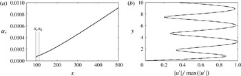
The absence of non-parallel effects in the Orr–Sommerfeld/Squire problem leads to a small transient when using the modes as an initial condition for the PSE marching (see e.g. Herbert Reference Herbert1994). This effect is visualized in figure 1(a) which shows the real part of the streamwise wavenumber of a single mode as a function of the streamwise coordinate. A comparison of the original eigenfunction at $x_{e}$ and the marched PSE solution at $x_{0}$ is provided in figure 1(b) and shows that the two solutions are virtually identical.

Figure 1.

(a) Real part of the streamwise disturbance wavenumber of an eigenfunction with $\unicode[STIX]{x1D6FD}=1.8$ , $\unicode[STIX]{x1D714}=0.01$ , computed by PSE marching starting from a spatial Orr–Sommerfeld eigenfunction at $x_{e}$ . (b) Absolute of the streamwise component of the eigenfunction computed via the solution of the eigenvalue problem at $x_{e}$ (solid) and via PSE marching from $x_{e}$ to $x_{0}$ (dashed).

The computational effort of the optimization procedure is reduced by exploiting the rapid convergence of $G$ under an expansion of the optimal disturbance, $\boldsymbol{h}_{0}$ , in terms of eigenfunctions of the spatial Orr–Sommerfeld problem. The underlying rationale is that the most stable modes decay so quickly that they are in essence irrelevant to the transient amplification of disturbances (see e.g. Reddy & Henningson Reference Reddy and Henningson1993). Considering only the $k$ least stable eigenfunctions, the optimal initial condition can be written as,

Here, the columns of $\unicode[STIX]{x1D64C}_{0}\;\in \mathbb{C}^{4n\times k}$ are the $k$ eigenfunctions, $\hat{\boldsymbol{q}}(x_{0},y)\exp (\text{i}\int _{x_{e}}^{x_{0}}\unicode[STIX]{x1D6FC}(\unicode[STIX]{x1D709})\,\text{d}\unicode[STIX]{x1D709})$ , $n$ is the number of grid points in the wall-normal dimension and $\unicode[STIX]{x1D73F}\in \mathbb{C}^{k\times 1}$ are the weights of the individual modes. Similarly, the solution at the final position is

with the columns of $\unicode[STIX]{x1D64C}_{1}$ representing the solutions obtained from evolving the $k$ eigenfunctions in $\unicode[STIX]{x1D64C}_{0}$ from $x_{0}$ to $x_{1}$ . Since the geometric multiplicity of the eigenfunctions of the Orr–Sommerfeld/Squire system is one, the operator $\unicode[STIX]{x1D64C}_{0}$ has full column rank, $\text{rk}\,\unicode[STIX]{x1D64C}_{0}=k~\forall ~k\in [1,4n]$ , and $\unicode[STIX]{x1D64C}_{0}^{\unicode[STIX]{x1D643}}\unicode[STIX]{x1D64C}_{0}$ is invertible. The Moore–Penrose pseudo-inverse of $\unicode[STIX]{x1D64C}_{0}$ is hence explicitly defined as

The full column rank of $\unicode[STIX]{x1D64C}_{0}$ further implies that $\unicode[STIX]{x1D64C}_{0}^{+}$ is a left inverse, so that $\unicode[STIX]{x1D64C}_{0}^{+}\unicode[STIX]{x1D64C}_{0}\equiv \unicode[STIX]{x1D644}$ , and specifically,

The matrix $\widetilde{\unicode[STIX]{x1D647}}_{k}\equiv \unicode[STIX]{x1D64C}_{1}\unicode[STIX]{x1D64C}_{0}^{+}$ thus defines an exact pseudo-fundamental solution operator which advances arbitrary superpositions of the first $k$ eigenfunctions from $x_{0}$ to $x_{1}$ . The solution to the optimization problem in terms of the $k$ modes is therefore

where the energy–weight matrix $\unicode[STIX]{x1D641}$ is defined such that $\Vert \unicode[STIX]{x1D641}\boldsymbol{h}\Vert _{2}\equiv \Vert \boldsymbol{h}\Vert _{E}$ . The 2-norm in the rightmost expression of (2.13) is equivalent to the spectral norm of $\unicode[STIX]{x1D641}\widetilde{\unicode[STIX]{x1D647}}_{k}\unicode[STIX]{x1D641}^{-1}$ and is efficiently computed via singular value decomposition.

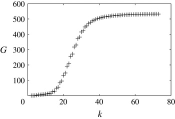
The influence of the length of the eigenfunction expansion, $k$ , on the energy gain is visualized in figure 2. Beyond $k\gtrsim 40$ , the energy amplification ratio converges increasingly to an asymptotic value of $G\approx 530$ . Assuming a total of 40 modes in the optimization procedure, the computational cost is thus comparable to 20 iterations in an adjoint-based scheme.

Figure 2.

Energy amplification ratio $G$ versus number of modes $k$ for parameters $\unicode[STIX]{x1D714}=10^{-6}$ , $\unicode[STIX]{x1D6FD}=1.8$ , $Re_{0}=2440$ .

The above optimization scheme based on the individual spatial evolution of the constituent eigenfunctions of the optimal disturbance is suitable for two- and three-dimensional base states. It avoids some of the restrictions of adjoint-based PSE approaches which evolve the total optimal disturbance by imposing a single streamwise wavenumber (e.g. Tempelmann, Hanifi & Henningson Reference Tempelmann, Hanifi and Henningson2010). Specifically when the optimal is described by a superposition of modes with varying streamwise wavenumber, such as eigenfunctions from both the discrete and continuous spectra, their simultaneous marching in the adjoint-based approach does not guarantee the accurate capturing of their individual evolution and by extension of the optimal disturbance as a whole (see also Towne Reference Towne2016).

Furthermore, the present algorithm does not require a priori knowledge of the streamwise wavenumber of the optimal disturbance. Instead, its streamwise form emerges naturally from the evolution of the constituent modes. The method further allows the efficient evaluation of any $G(x_{0},x_{1}^{\prime })$ with $x_{0}<x_{1}^{\prime }<x_{1}$ . Storing the intermediate spatial history of the PSE solution between $x_{0}$ and $x_{1}$ enables the immediate construction of $\widetilde{\unicode[STIX]{x1D647}}_{k}(x_{0},x_{1}^{\prime })$ , and the optimization problem is reduced to a re-evaluation of the SVD. This property is advantageous when the interest is in computing the globally most highly energetic perturbations for a given Reynolds number, maximized over all possible final positions.

3 Non-parallel optimal disturbances

In the following, results on the spatial growth of disturbances in non-parallel Blasius boundary layers, computed with the above described optimization framework, are presented. The first set-up considers the most highly amplified perturbations due to non-modal mechanisms for a constant initial position $x_{0}=108$ , corresponding to a Reynolds number $Re=2440$ . The gain in the kinetic energy of the perturbations is maximized over all final positions,

Since the focus is on purely algebraic perturbation growth, the region of small $\unicode[STIX]{x1D6FD}$ where an interaction of non-modal growth with the exponential Tollmien–Schlichting waves can occur (see Åkervik et al. Reference Åkervik, Ehrenstein, Gallaire and Henningson2008) is excluded from the analysis.

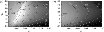
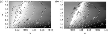
The maximum energy gain as a function of the disturbance frequency and the spanwise wavenumber is presented in figure 3(a). A band of high disturbance amplification is observed which approximately stretches from $\unicode[STIX]{x1D6FD}=1.0$ , $\unicode[STIX]{x1D714}=0.013$ to $\unicode[STIX]{x1D6FD}=3.5$ and $\unicode[STIX]{x1D714}=0.040$ . The global maximum of $G\approx 1.5\times 10^{4}$ occurs at parameters $\unicode[STIX]{x1D6FD}=1.8$ and $\unicode[STIX]{x1D714}=0.023$ . For reference, figure 3(b) shows the perturbation energy gain computed with the spatial PSE scheme, however under the assumption of a parallel base flow, i.e. by setting $U(x,y)\equiv U(x_{0},y)$ and $V(x,y)\equiv 0$ . The parallel results indicate a significantly lower global maximum of $G=1031$ , in line with the value of $G_{t}=980$ predicted by the scaling law derived from the temporal parallel-flow analysis of Butler & Farrell (Reference Butler and Farrell1992). In agreement with the existing literature, the most highly amplified perturbations in the parallel flow have zero frequency and a spanwise wavenumber of $\unicode[STIX]{x1D6FD}\approx 1.8$ based on the boundary-layer thickness at $x_{0}$ . In the non-parallel case, the energy gain at these parameter is $G=1046$ , indicating that the expansion of the boundary layer has a rather limited effect on perturbations with extremely low frequency.

Figure 3.

Maximum energy amplification ratio $G$ (logarithmic scaling) at $Re_{0}=2440$ as a function of the perturbation frequency $\unicode[STIX]{x1D714}$ and the perturbation wavenumber $\unicode[STIX]{x1D6FD}$ . (a) Non-parallel flow. (b) Parallel flow.

Figure 4.

Streamwise coordinate $x_{1}$ of the highest perturbation kinetic energy at $Re_{0}=2440$ as a function of the perturbation frequency $\unicode[STIX]{x1D714}$ and the perturbation wavenumber $\unicode[STIX]{x1D6FD}$ . (a) Non-parallel flow. (b) Parallel flow.

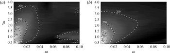
Contours of the streamwise location of highest perturbation kinetic energy, $x_{1}$ , are provided in figure 4. The results show that the most highly energetic perturbations are observed between $x=200$ and $x=250$ , i.e. approximately $100$ – $150$ boundary-layer thicknesses downstream of the initial position, $x_{0}=108$ . The parallel-flow case presented in figure 4(b) provides a similar outcome, substantiating that non-parallel effects only marginally change the length scales of non-modal perturbation growth.

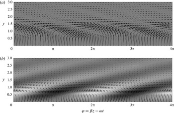
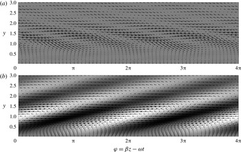
The involvement of the Orr mechanism in the evolution of the most highly amplified disturbances becomes clear from visualizations of the solution as a function of the phase, $\unicode[STIX]{x1D711}=\unicode[STIX]{x1D6FD}z-\unicode[STIX]{x1D714}t$ , at the initial and final positions of the optimization scheme, see figure 5. At a location of constant spanwise coordinate $z$ , the abscissa describes the variation of the disturbance field with time. Analogously, at a specific time instance $t$ , the axis indicates the change of the perturbation field in the spanwise dimension. The initial field at $x_{0}$ is presented in figure 5(a). While the streamwise component has negligible amplitude, the spanwise and normal components form vortices which are tilted against the direction of the mean shear. At the final position (figure 5 b), the vortices have been reoriented by the base flow. Simultaneously, the vortices have caused an amplification of the streamwise perturbation component according to the classical lift-up mechanism. The present results thus substantiate and quantify findings in global optimal growth analyses, for instance by Monokrousos et al. (Reference Monokrousos, Åkervik, Brandt and Henningson2010), where a reorientation of perturbations that were initially tilted against the shear was reported. Their results also indicated that the most highly amplified disturbances in non-parallel flows are spatially compact and have finite length.

Figure 5.

Optimal disturbance as a function of the phase $\unicode[STIX]{x1D711}=\unicode[STIX]{x1D6FD}z-\unicode[STIX]{x1D714}t$ . Contours of the streamwise component with vectors of the spanwise and normal components. (a) Initial position, $x_{0}=108$ . (b) Position of highest kinetic energy, $x_{1}=250$ .

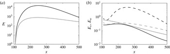
The total perturbation kinetic energy, $E(x)\equiv \Vert \boldsymbol{q}(x)\Vert _{E}$ , as a function of the streamwise coordinate at parameters $\unicode[STIX]{x1D6FD}=1.8$ , $\unicode[STIX]{x1D714}=0.02$ is evaluated in figure 6(a) for the parallel and non-parallel cases. The results show an additional energy gain of the total energy in the non-parallel flow, followed by a more rapid viscous decay than observed in the parallel case. Results for the energy in the normal and transverse components presented in figure 6(b) demonstrate that non-parallel effects introduce an appreciable amplification of $E_{w}$ . This additional amplification of the energy in the spanwise component can be ascribed to an Orr mechanism in the cross-plane, see figure 5, which is augmented by the non-uniform $V(y)$ absent in parallel flow. On the other hand, the normal component remains at the same or a lower level in the non-parallel case, indicating that the additional energy gain is not due to an enhanced lift-up mechanism via stronger normal displacement of the mean momentum. We note that in both cases, the kinetic energy in the normal and spanwise perturbations remains several orders of magnitude smaller than in the streamwise perturbation component which at the peak of $E(x)$ makes up more than $99.9\,\%$ of the total kinetic energy in both the non-parallel and parallel cases.

Figure 6.

Perturbation kinetic energy as a function of streamwise coordinate at $\unicode[STIX]{x1D6FD}=1.8$ , $\unicode[STIX]{x1D714}=0.02$ . Non-parallel flow (black) and parallel flow (grey). (a) Total kinetic energy, $E$ . (b) Energy in the normal component, $E_{v}$ , (solid) and in the spanwise component, $E_{w}$ (dashed).

Figure 7.

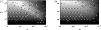
Maximum energy amplification ratio $G$ (logarithmic scaling) at $Re_{0}=2440$ as a function of the perturbation frequency $\unicode[STIX]{x1D714}$ and the Reynolds number $Re$ . (a) Non-parallel flow. (b) Parallel flow.

The initial position and thus the Reynolds number of the analysis have been kept constant so far. In the remainder of this section, we aim to establish the influence of $Re$ on algebraic growth in non-parallel boundary layers. Since algebraic growth is only limited by viscosity, the general trend of stronger growth with higher Reynolds number can also be expected to prevail in non-parallel flow. Contours of the energy amplification factor as a function of $\unicode[STIX]{x1D714}$ and $Re$ , presented in figure 7(a), support this surmise. The global maximum of $G$ within the considered parameter range is observed at the largest investigated Reynolds number, $Re=2.2\times 10^{5}$ , at a finite frequency $\unicode[STIX]{x1D714}\approx 4\times 10^{-4}$ . In line with the literature on temporal optimal disturbances (e.g. Butler & Farrell Reference Butler and Farrell1992), the optimal frequency in the parallel case presented in figure 7(b) is zero for all Reynolds numbers.

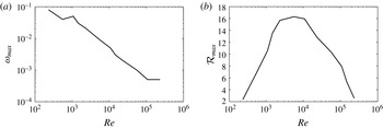
The frequency at which non-modal growth is most effective can be intuitively related to the interaction of the Orr and lift-up mechanisms. The tilting of flow structures by the mean shear in the Orr mechanism requires a finite perturbation length scale and is inactive in the case of zero-frequency perturbations which however maximize the efficiency of the lift-up process. In figure 8(a), the frequency of the most highly amplified perturbations is plotted versus $Re$ . Larger Reynolds numbers are observed to favour lower perturbation frequencies and thus increase the relevance of lift-up at the expense of the Orr mechanism. With logarithmic scaling for both axes, the relation can be approximated by a straight line, indicating a power law $\unicode[STIX]{x1D714}_{max}\sim Re^{-\unicode[STIX]{x1D701}}$ with $\unicode[STIX]{x1D701}\approx 0.8$ . An extrapolation of this trend predicts the most highly amplified perturbations to have zero frequency as $Re\rightarrow \infty$ , consistent with the vanishing of non-parallel effects in the inviscid limit.

Finally, the magnitude of the energy amplification is compared between the parallel and non-parallel cases by evaluating the amplification ratio

which relates the values obtained for $G$ , maximized over all end points and frequencies at a given $x_{0}$ and thus $Re$ . The result, presented in figure 8, shows a distinct maximum for ${\mathcal{R}}_{max}$ near $Re\approx 10^{4}$ where non-parallel effects extremally enhance algebraic growth through the interaction of Orr and lift-up mechanisms. The result suggests that in the relatively viscous regime at small $Re$ where the gain due to algebraic growth is small, non-parallel effects are relatively ineffective at enhancing the amplification of disturbances. The decay at large $Re$ is consistent with the aforementioned absence of non-parallel effects in the limit of large Reynolds numbers.

Figure 8.

(a) Frequency $\unicode[STIX]{x1D714}_{max}$ of most highly amplified perturbations as a function of the Reynolds number. (b) Ratio ${\mathcal{R}}_{max}$ of the energy amplification factors of non-parallel and parallel flow as a function of the Reynolds number.

4 Streamwise pressure gradient

Several earlier studies have examined the effect of a streamwise pressure gradient on the non-modal growth of perturbations in boundary layers. Temporal optimal growth analyses in parallel flow by Corbett & Bottaro (Reference Corbett and Bottaro2000) showed that adverse pressure gradient (APG) can lead to stronger algebraic amplification. Consistent with parallel analyses of the Blasius boundary layer, their results predicted that the most highly amplified perturbations have zero streamwise wavenumber, independent of the Reynolds number. For short suboptimal time intervals, the most highly amplified disturbances were however characterized by finite streamwise wavenumbers. Linear parallel analyses and nonlinear direct simulations by Zaki & Durbin (Reference Zaki and Durbin2006) led to commensurate results of stronger streaks in the presence of adverse pressure gradient. Stability analyses of streaky boundary layers by Hack & Zaki (Reference Hack and Zaki2014) showed that adverse pressure gradient can also enhance the secondary instability of streaks, explaining the early breakdown to turbulence observed in APG boundary layers. More recently, Hack & Zaki (Reference Hack and Zaki2016) demonstrated that the local momentum thickness can act as a similarity parameter across pressure gradients for several attributes of boundary-layer streaks including their amplitude and cross-sectional area.

In the following, we extend the analysis of non-parallel optimal perturbations to boundary layers with streamwise pressure gradient. Both an adverse- and a favourable-pressure-gradient (FPG) case with respective Hartree parameters $H=-0.10$ and $H=0.10$ are considered. The streamwise and normal base flow is modelled via the Falkner–Skan equations (see e.g. Schlichting & Gersten Reference Schlichting and Gersten2006) with the free-stream velocity following a power law,

where the constant $C$ was chosen such that $U(x_{0},y\rightarrow \infty )=1$ . The exponents are $m=-0.0476$ in the APG case and $m=0.0526$ in the FPG case. It is worth mentioning that the variation of the free-stream convective speed in $x$ , i.e. in the dimension in which the disturbances evolve, is in contrast to temporal analyses, which capture the effect of the pressure gradient only through the (invariable) shape of the base-flow profile. In the following, we scale the amplitudes of the disturbances with $U(x_{0},y\rightarrow \infty )$ . The alternative normalization by the local free-stream speed predicts weaker amplification in the FPG case and higher amplification in the APG case.

Figure 9.

Maximum energy amplification ratio $G$ (logarithmic scaling) at $Re_{0}=2440$ as a function of the perturbation frequency $\unicode[STIX]{x1D714}$ and the perturbation wavenumber $\unicode[STIX]{x1D6FD}$ . (a) Adverse pressure gradient. (b) Favourable pressure gradient.

The most highly amplified perturbations at Reynolds number $Re_{0}=2440$ , corresponding to initial positions $x_{0}=88.1$ (APG) and $x_{0}=137.4$ (FPG), are considered. Analogous to the ZPG flow, the energy gain is again maximized over all possible final positions $x_{1}$ . Results for $G$ in both flow configurations as a function of the spanwise disturbance wavenumber and the disturbance frequency are presented in figure 9. Adverse gradient enhances the algebraic amplification of disturbances with a global maximum of $G\approx 4.3\times 10^{4}$ , approximately three times the value found for the ZPG boundary layer. Similar to the Blasius case, the most highly amplified disturbances in both configurations are again found in a limited region of non-zero frequency that is aligned at an angle in the frequency/wavenumber plane. The most energetic perturbations in the APG case are generated at parameters $\unicode[STIX]{x1D6FD}=1.8$ and $\unicode[STIX]{x1D714}=0.01625$ . The amplification takes place over the distance $\unicode[STIX]{x0394}x=x_{1}-x_{0}=41.8$ which is considerably shorter than the distance $\unicode[STIX]{x0394}x=141.8$ of the most highly amplified disturbances in the ZPG case at the same Reynolds number. In line with the existing literature on parallel-flow, comparison with the ZPG case also shows that perturbations with zero frequency are weaker in the FPG case and stronger in the APG boundary layer.

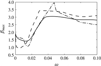
The relation between the scales of the perturbations preferentially generated by algebraic growth is quantified in figure 10. The ordinate indicates the spanwise wavenumber of the most highly amplified disturbances, $\unicode[STIX]{x1D6FD}_{max}$ , as a function of their frequency. All three considered flow configurations show linear trends in the region of highest amplification $0.015\lesssim \unicode[STIX]{x1D714}\lesssim 0.04$ . In particular, the slope of the curves is similar in all cases, although shifted to lower frequencies in the adverse pressure gradient.

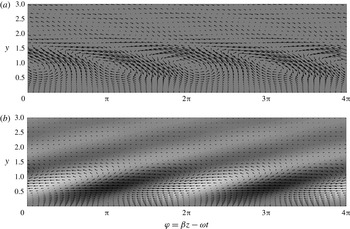
Visualizations of the most highly amplified disturbances in the APG boundary layer as a function of the phase are presented in figure 11. Similar to the Blasius case, the most energetic perturbations are generated by a combination of the Orr and lift-up mechanisms. At the initial position, the disturbances are tilted to the left at approximately the same angle in the $\unicode[STIX]{x1D711}$ – $y$ plane as in the ZPG boundary layer. While the amplification takes place over a shorter distance, the reorientation and thus the angle at $x_{1}$ is again comparable to the Blasius case.

Figure 10.

Spanwise wavenumber of the most highly amplified perturbations as a function of the perturbation frequency $\unicode[STIX]{x1D714}$ at $Re=2440$ . ZPG (black), APG (dashed) and FPG (dash-dotted).

Figure 11.

Optimal disturbance in APG boundary layer as a function of the phase $\unicode[STIX]{x1D711}=\unicode[STIX]{x1D6FD}z-\unicode[STIX]{x1D714}t$ . Contours of the streamwise component with vectors of the spanwise and normal components. (a) Initial position, $x_{0}=88.1$ . (b) Position of highest kinetic energy, $x_{1}=129.7$ .