1 Introduction
During a balanced flight, e.g. hovering, an insect must produce enough lift to balance its weight. Due to an insect’s small size, the relative velocity of the flapping wing is low. Therefore, the required lift coefficient of the wing is relatively high (Ellington Reference Ellington1984a,Reference Ellingtonb,Reference Ellingtonc,Reference Ellingtond); the mean lift coefficient required is 1.5–2 (Ellington Reference Ellington1984d; Liu et al. Reference Liu, Ellington, Kawachi, van den Berg and Willmott1998; Sun & Du Reference Sun and Du2003; Fry, Sayaman & Dickinson Reference Fry, Sayaman and Dickinson2005), about three times as large as that of an airplane at cruising flight. On the other hand, because both the wing size and the wing speed are small, the Reynolds number ( $Re$) of the wing is small;
 $Re$ ranges from about 10 (Encarsia Formosa: Weis-Fogh (Reference Weis-Fogh1973)) to 3500 (Hawkmoths: Ellington (Reference Ellington1984b), Sun & Du (Reference Sun and Du2003)) (in the present paper,
 $Re$ is based on the mean chord length of the wing and the mean speed at the radius of gyration of the wing). In this low
 $Re$ range, conventional steady-state aerodynamic theory is insufficient to explain the required high aerodynamic-force coefficients and unsteady aerodynamic mechanisms must be operating (Ellington Reference Ellington1984c). Several unsteady mechanisms have been proposed to explain the high aerodynamic-force coefficients. Among them are the ‘clap and fling’ (Lighthill Reference Lighthill1973; Weis-Fogh Reference Weis-Fogh1973), the ‘delayed stall’ (Ellington et al. Reference Ellington, Van Den Berg, Willmott and Thomas1996; Liu et al. Reference Liu, Ellington, Kawachi, van den Berg and Willmott1998; Dickinson, Lehmann & Sane Reference Dickinson, Lehmann and Sane1999; Bomphrey et al. Reference Bomphrey, Srygley, Taylor and Thomas2002), the pitching-up rotation near the end of a downstroke or upstroke (Dickinson et al. Reference Dickinson, Lehmann and Sane1999; Sun & Tang Reference Sun and Tang2002) and the fast acceleration (or added mass) at the beginning of a downstroke or upstroke (Sun & Tang Reference Sun and Tang2002; Sane Reference Sane2003).
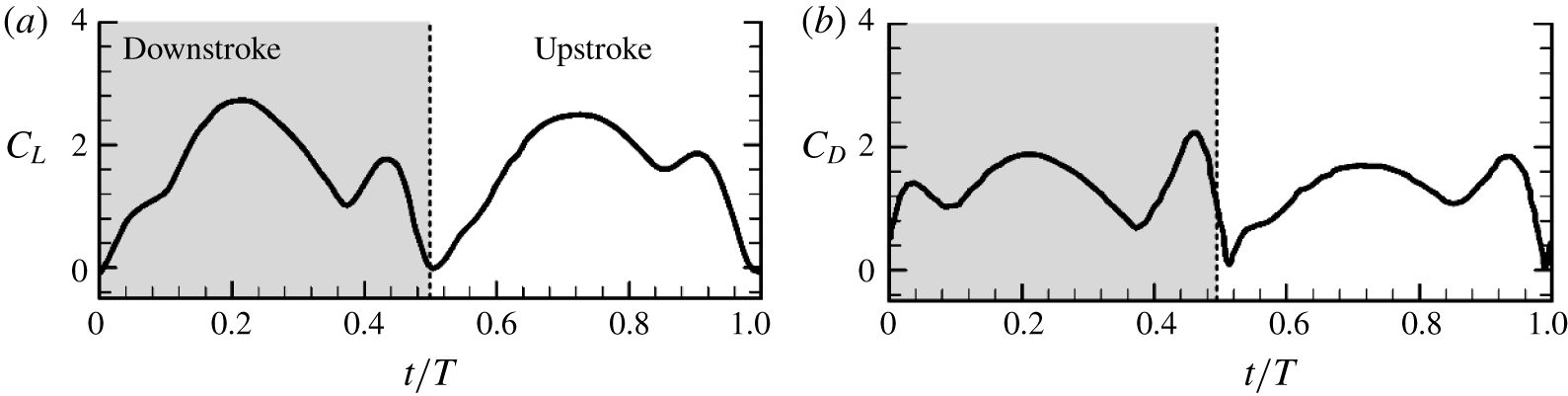
For many insects in normal hovering (wings flap in an approximately horizontal plane and stroke amplitude is around  $120^{\circ }$ or larger) it has been shown that the lift and drag of the wing generally have three peaks in a downstroke or upstroke (Wang, Birch & Dickinson Reference Wang, Birch and Dickinson2004; Fry et al. Reference Fry, Sayaman and Dickinson2005; Aono, Liang & Liu Reference Aono, Liang and Liu2008; Liu & Sun Reference Liu and Sun2008; Han, Chang & Han Reference Han, Chang and Han2016), an example being shown in figure 1 (in the figure
 $C_{L}$ and
 $C_{D}$ are the lift and drag coefficients, respectively;
 $t$ is the time and
 $T$ is the flapping period). The force peak in the beginning of the downstroke
 $(t/T=0{-}0.5)$ or upstroke
 $(t/T=0.5{-}1)$ is produced by the fast acceleration (or added-mass) mechanism. The ‘wider’ force peak in the mid-portion of the downstroke or upstroke is due to the delayed-stall mechanism, i.e. the leading-edge vortex (LEV) attached to and moving with the wing. The force peak near the end of the downstroke or upstroke is generated by the wing pitching-up rotation mechanism. The peak in the mid-portion of the downstroke or upstroke due to the delayed-stall mechanism provides approximately 60 %–70 % of the stroke-cycle mean lift (Liu & Sun Reference Liu and Sun2008; Lee, Choi & Kim Reference Lee, Choi and Kim2015).
Lift and drag coefficients of a dronefly in a flapping period (adopted from Liu & Sun (Reference Liu and Sun2008)).

Mosquitoes also conduct normal hover flight, but their stroke amplitude (about  $45^{\circ }$) is much lower than that of other insects (Dickerson et al. Reference Dickerson, Shankles, Madhavan and Hu2012, Reference Dickerson, Shankles, Berry and Hu2015). Recently, Bomphrey et al. (Reference Bomphrey, Nakata, Phillips and Walker2017) studied the aerodynamics of the hovering mosquito Culex quinquefasciatus through measuring the wing motion and simulating the flows around the insect. The wing stroke amplitude is around
 $45^{\circ }$ and
 $Re$ is about 70. Their results show that similar to the case of insects with large stroke amplitude, the lift and drag generally have three peaks in a downstroke or upstroke: one in the beginning, one in the mid-portion and one near the end of the downstroke or upstroke (in some cases, the force peak in the mid-portion and that near the end may combine into one force peak because the pitch rotation near the end of the downstroke or upstroke starts earlier). The authors suggested the following explanations for the three forces peaks: the force peak at the beginning of the downstroke or upstroke was due to a vortex near the trailing edge caused by the wing encountering the flow of the previous stroke (wake capture); the force peak in the mid-portion of the downstroke or upstroke was attributed to the well-known leading-edge vortex (i.e. the delayed-stall mechanism); and the force peak near the end of the downstroke or upstroke was explained by the wing rotation mechanism.
Previous studies on insect flight showed that the wake from a previous stroke has detrimental effects on aerodynamic-force generation in the beginning of a downstroke or upstroke (Sun & Tang Reference Sun and Tang2002; Meng & Sun Reference Meng and Sun2015), and that for small-amplitude flapping, the leading-edge vortex does not have enough time to form and the delayed-stall mechanism cannot play a role in aerodynamic-force generation (e.g. Wang et al. Reference Wang, Birch and Dickinson2004; Harbig, Sheridan & Thompson Reference Harbig, Sheridan and Thompson2013; Eldredge & Jones Reference Eldredge and Jones2019). Therefore, the force peaks in the beginning and in the mid-portion of the downstroke or upstroke might not be correctly explained in the Bomphrey et al. (Reference Bomphrey, Nakata, Phillips and Walker2017) paper.
The non-dimensional Navier–Stokes equations that govern the flows around the wing are
 $$\begin{eqnarray}\displaystyle & \displaystyle \unicode[STIX]{x1D735}\boldsymbol{\cdot }\boldsymbol{u}=0, & \displaystyle\end{eqnarray}$$
 $$\begin{eqnarray}\displaystyle & \displaystyle St\frac{\unicode[STIX]{x2202}\boldsymbol{u}}{\unicode[STIX]{x2202}\unicode[STIX]{x1D70F}}+\boldsymbol{u}\boldsymbol{\cdot }\unicode[STIX]{x1D735}\boldsymbol{u}=-\unicode[STIX]{x1D735}p+\frac{1}{Re}\unicode[STIX]{x1D6FB}^{2}\boldsymbol{u}, & \displaystyle\end{eqnarray}$$
where  $\boldsymbol{u}$ and
 $p$ are the non-dimensional flow velocity and pressure, respectively,
 $\unicode[STIX]{x1D70F}$ is the non-dimensional time and
 $St$ and
 $Re$ are the Strouhal number and Reynolds number, respectively; in non-dimensionalization, the mean chord length
 $c$ is the reference length, the mean flapping velocity at the radius of gyration of the wing
 $U$ is the reference velocity (
 $U=2\unicode[STIX]{x1D6F7}fr_{2}$, where
 $\unicode[STIX]{x1D6F7}$ is the stroke amplitude,
 $f$ the stroke frequency and
 $r_{2}$ the radius of gyration of the wing) and the stroke period
 $T=1/f$ is the reference time. The parameter representing the unsteady effect,
 $St\,(=c/\unicode[STIX]{x1D6F7}r_{2})$, is very large when
 $\unicode[STIX]{x1D6F7}$ is very small. That is, the flow around the mosquito wing is highly unsteady. The explanations of the force peaks in the beginning and in the mid-portion of the downstroke or upstroke by Bomphrey et al. (Reference Bomphrey, Nakata, Phillips and Walker2017) were mainly based on the instantaneous flow streamline patterns. In a highly unsteady flow, an instantaneous streamline pattern can be very different from the vortex pattern. Moreover, the role of added mass was not clarified in the Bomphrey et al. (Reference Bomphrey, Nakata, Phillips and Walker2017) study, which may be very important for the very unsteady flow of the mosquito wing.
In the present paper we will study the flow physics in detail and reveal the unsteady force production mechanisms of hovering mosquitoes, by numerically solving the Navier–Stokes equations and by applying the vortex dynamics theory and the theory of added mass to the analysis of the flows. In the Bomphrey et al. (Reference Bomphrey, Nakata, Phillips and Walker2017) paper, animal weight was not measured in their experiment; whether or not the computed lift balances the weight cannot be checked. In the present work, we will first measure the wing kinematics and the morphological parameters (including the weight of the insects) and then conduct the flow analysis.
2 Measurement of the wing kinematics
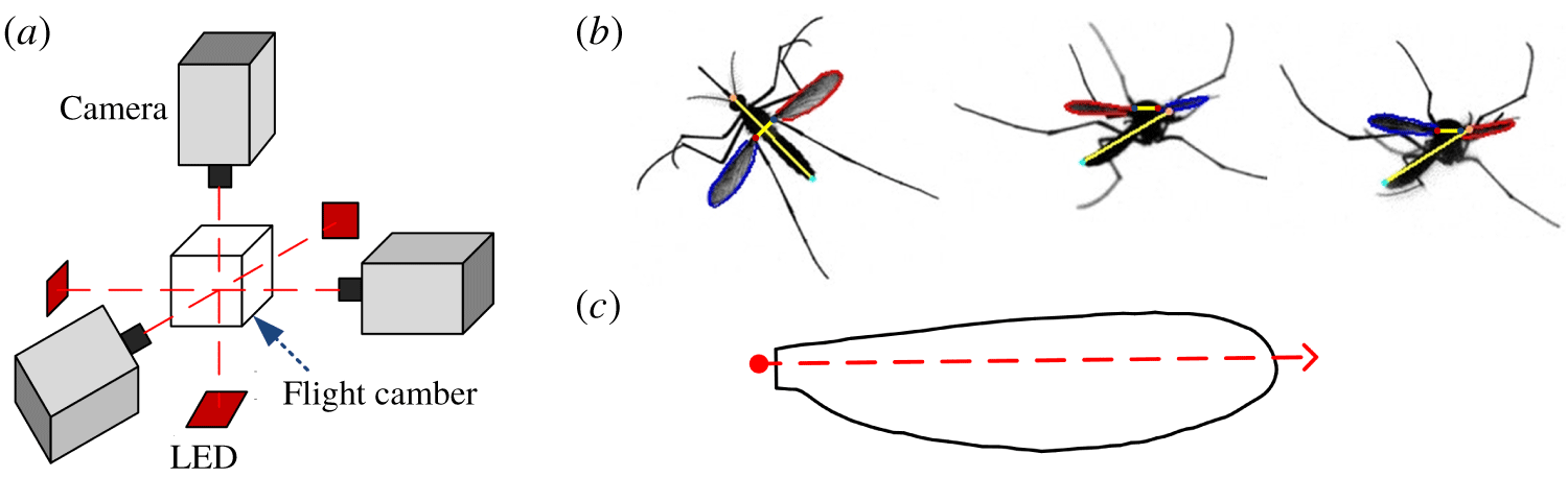
Wing motion and morphological parameters of mosquito Aedes aegypti in hovering flight were measured. The flight of the insect was filmed by three high-speed cameras (figure 2a) and wing kinematics is extracted from the filmed data (figure 2b). Immediately after filming the insect was killed with ethyl acetate vapour and morphological parameters such as the wing shape (figure 2c), the total mass, etc. were measured. Descriptions of the measurement process and the relevant methods are given in appendix A.
(a) Experimental setup. (b) Graphs illustrating the extraction of kinematic data from the filmed data. (c) The wing shape.

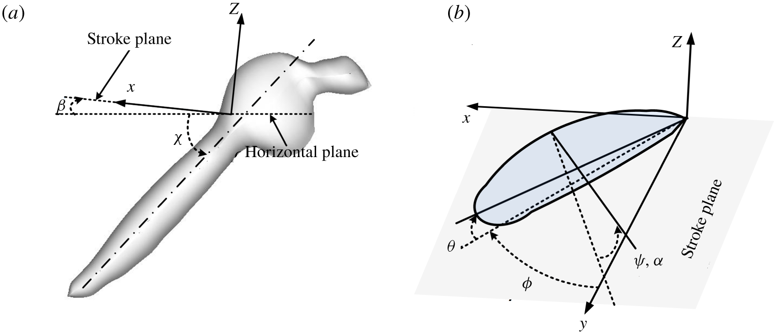
The reference frame and the angles defining the wing kinematics.

Flight data of eight mosquitoes were obtained. The insects are named as M1, M2, M3, M4, M5, M6, M7 and M8, respectively (M1, M2, M3 and M4 are female and M5, M6, M7 and M8 are male). As an example, video sequences for M1 and M5 are given as movies 1 and 2 in the supplementary material available at https://doi.org/10.1017/jfm.2020.386. In order to describe the wing kinematics, we introduce the stroke plane and a reference frame as follows. For each mosquito, data of 30 wingbeat cycles were processed. The wing-tip points of both the left and right wings were projected on to the plane of symmetry of the insect and a linear regression line of the projection was then determined. The plane which passed the wing root and was parallel to the line was defined as the stroke plane (figure 3). Let  $(x,y,z)$ be the reference frame; its origin is at the wing root,
 $x{-}y$ plane is in the stroke plane, with
 $y$ pointing to the right side of the insect, and
 $z$ is perpendicular to the stroke plane, pointing upwards (figure 3). The angle between the stroke plane and the horizontal (
 $\unicode[STIX]{x1D6FD}$, figure 3a) is referred to as the stroke plane angle. For most hovering insects, the stroke plane is approximately horizontal and
 $\unicode[STIX]{x1D6FD}$ is very small. If the wing is rigid, the flapping motion could be described by three Euler angles (the positional angle,
 $\unicode[STIX]{x1D719}$; the deviation angel,
 $\unicode[STIX]{x1D703}$; and the pitch angle,
 $\unicode[STIX]{x1D713}$). But the mosquitoes have slender wings and the wing will have spanwise change in pitch angle (wing twist) during the flapping motion. The spanwise change in pitch angle is approximately linear (see appendix A). Thus, the flapping motion of the wing can be described by three Euler angles:
 $\unicode[STIX]{x1D719}$,
 $\unicode[STIX]{x1D703}$ and
 $\unicode[STIX]{x1D713}$ at the radius of gyration of the wing (figure 3b), and a quantity representing the spanwise change in pitch angle. For convenience, we introduce the angle of attack (
 $\unicode[STIX]{x1D6FC}$) to replace the pitch angle;
 $\unicode[STIX]{x1D6FC}$ is related to
 $\unicode[STIX]{x1D713}$ as follows:
 $\unicode[STIX]{x1D6FC}=\unicode[STIX]{x1D713}$ in the downstroke and
 $\unicode[STIX]{x1D6FC}=180^{\circ }$–
 $\unicode[STIX]{x1D713}$ in the upstroke. In the present paper, the quantity representing the spanwise change in pitch angle is the difference between
 $\unicode[STIX]{x1D6FC}$ at the wing root and that at the wing tip and is denoted as
 $\unicode[STIX]{x0394}\unicode[STIX]{x1D6FC}_{tw}$. Hereafter,
 $\unicode[STIX]{x0394}\unicode[STIX]{x1D6FC}_{tw}$ is called as spanwise change in angle of attack (or spanwise change in
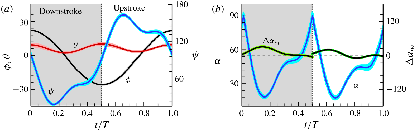
 $\unicode[STIX]{x1D6FC}$). The measured results of these angles for M1 are shown in figure 4, given as mean values
 $\pm$ standard deviation (s.d.); those of the other seven mosquitoes are given in appendix B (figure 22).
Measured Euler angles,  $\unicode[STIX]{x1D719}$,
 $\unicode[STIX]{x1D703}$ and
 $\unicode[STIX]{x1D713}$ (or
 $\unicode[STIX]{x1D6FC}$), and the spanwise change in
 $\unicode[STIX]{x1D6FC}$,
 $\unicode[STIX]{x0394}\unicode[STIX]{x1D6FC}_{tw}$; mean
 $\pm$ s.d. (
 $n=30$ wingbeats).

Flight data for the eight mosquitoes.

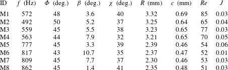
The wingbeat frequency  $(f)$, stroke amplitude (
 $\unicode[STIX]{x1D6F7}$; defined as the difference between the maximum and minimum
 $\unicode[STIX]{x1D719}$), Reynolds number (
 $Re$, defined in § 1) and the morphological parameters are given in table 1. In table 1
 $J$ is the advance ratio, the ratio between the forward flight speed and the mean tip speed
 $(2\unicode[STIX]{x1D6F7}fR)$. For an exact hover flight,
 $J=0$. It is commonly considered that when
 $J$ is less than 0.1, the insect is in approximate hover flight (Ellington Reference Ellington1984b) (
 $J$ can reach 0.9 or more when an insect is at fast flight, Meng & Sun (Reference Meng and Sun2016)). As seen in table 1, for the mosquitoes filmed in the present study,
 $J$ is very small:
 $J$ is not more than 0.05, except one mosquito, M5, whose
 $J$ is 0.06. Therefore, the mosquitoes are in approximate hover flight.
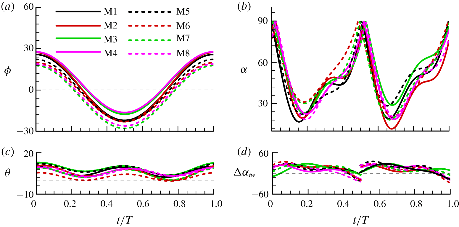
It is observed that the eight mosquitoes have similar flapping patterns (see figure 22 in appendix B). The mosquitoes are special in that they have a very small stroke amplitude and very high wingbeat frequency (table 1), as was found by previous studies of Dickerson et al. (Reference Dickerson, Shankles, Madhavan and Hu2012, Reference Dickerson, Shankles, Berry and Hu2015) and Bomphrey et al. (Reference Bomphrey, Nakata, Phillips and Walker2017). Dickerson et al. (Reference Dickerson, Shankles, Madhavan and Hu2012, Reference Dickerson, Shankles, Berry and Hu2015) did not measure the Euler angles. Bomphrey et al. (Reference Bomphrey, Nakata, Phillips and Walker2017) measured the Euler angles of 15 flight sequences, but the flapping patterns of many of the flight sequences are not very consistent. This can be seen from their calculated lift patterns in the extended data figure 8 in Bomphrey et al. (Reference Bomphrey, Nakata, Phillips and Walker2017): results of mosquitoes 8, 9 and 10 are similar; the results of the other 12 mosquitoes are qualitatively different from those of the above three mosquitoes (for example, mosquitoes 11 and 15 do not have a force peak in the mid-portion like that of mosquitoes 8–10). Because the insect weight was not measured in their experiment, whether or not the insects were in balanced hovering flight (lift equals to weight and total force is in the vertical direction) could not be checked. The inconsistency in their data might be because some of the mosquitoes were not in balanced hovering flight, but in some type of a transient flight.
Besides small stroke amplitude and high wingbeat frequency, another special feature is noticed in our results: in the mid-portion of a downstroke or upstroke ( $t/T\approx 0.12{-}0.34$ or
 $t/T\approx 0.62{-}0.84$, figure 4b), the angle of attack
 $\unicode[STIX]{x1D6FC}$ increases rapidly, pitching up from about
 $16^{\circ }$ to
 $46^{\circ }$. Note that, for insects with a large stroke amplitude,
 $\unicode[STIX]{x1D6FC}$ in the mid-portion of a downstroke or upstroke changes only slightly (Ellington Reference Ellington1984b; Fry et al. Reference Fry, Sayaman and Dickinson2005; Liu & Sun Reference Liu and Sun2008; Walker, Thomas & Taylor Reference Walker, Thomas and Taylor2010). The above
 $\unicode[STIX]{x1D6FC}$-motion feature of mosquitoes was not noticed previously and it plays an important role in aerodynamic-force generation, as will be shown in a later section (§ 4.2).
3 Computation of the flows and aerodynamic forces
The flows around and aerodynamic forces acting on the mosquito wing are computed by numerically solving the Navier–Stokes equations (1.1) and (1.2). The model wing has approximately the same platform as the mosquito wing (figure 2c) and the section of the model wing is a flat plate of 3 % thickness with rounded leading and trailing edges. The algorithm of solution is based on the method of artificial compressibility developed by Rogers, Kwak & Kiris (Reference Rogers, Kwak and Kiris1991) and the flow solver was developed by our group (Lan & Sun Reference Lan and Sun2001; Sun & Yu Reference Sun and Yu2006; Du & Sun Reference Du and Sun2008). The solver has been validated by comprehensive tests in our previous works (e.g. Cheng & Sun Reference Cheng and Sun2018): comparison has been made with the measured data of a revolving wing  $(Re=500)$ and a flapping wing
 $(Re=180)$; and comparison has been also made with theoretical (Stokes and Oseen solutions) and measured results for a sphere at very low
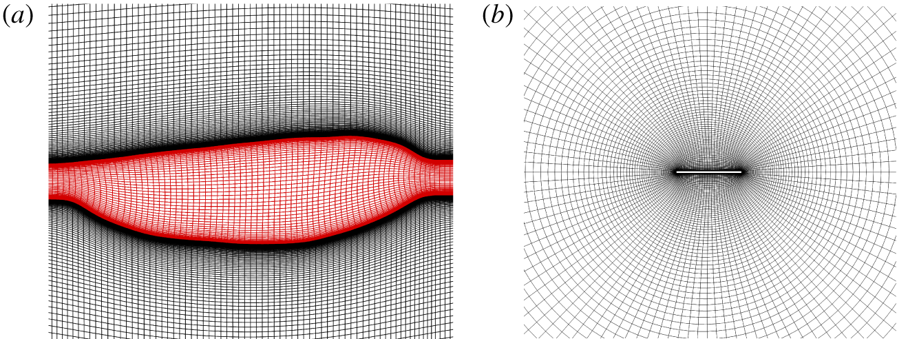
 $Re$ (5–20). A description of the computation is given in appendix A. The computational grids (O-H type) are generated using a Poisson solver, which is based on the work of Hilgenstock (Reference Hilgenstock, Sengupta, Hauster, Eiseman and Thompson1988). Portions of a computational grid are shown in figure 5. Tests on grid size, domain size and time step are given in appendix A.
The computational grid in the plane of wing planform (a) and that in a wing section (b).

Let  $C_{L}$ and
 $C_{D}$ denote the lift and drag coefficients of the wing, respectively. They are defined as
 $C_{L}=L/0.5\unicode[STIX]{x1D70C}U^{2}S$ and
 $C_{D}=D/0.5\unicode[STIX]{x1D70C}U^{2}S$, where
 $L$ and
 $D$ are the lift and drag, respectively, and
 $\unicode[STIX]{x1D70C}$ is the air density. The computed
 $C_{L}$ and
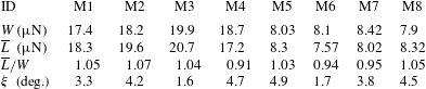
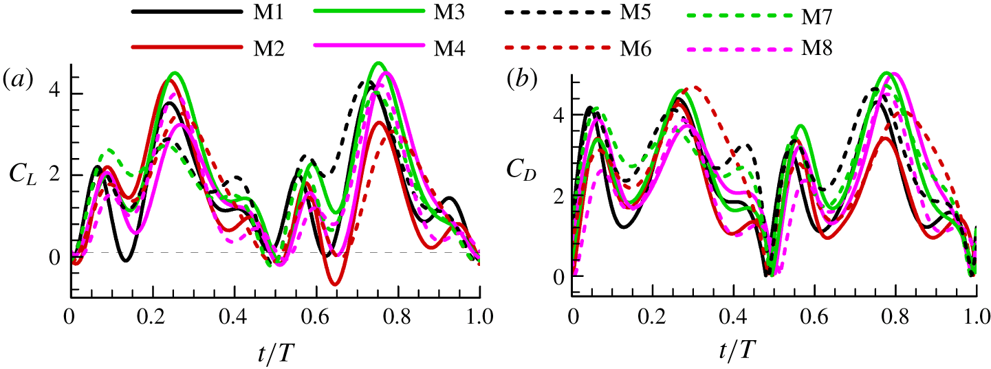
 $C_{D}$ for mosquito M1 are given in figure 6; the results for all the eight individuals are given in appendix B (figure 23). Since the insects are in hovering flight, the computed mean lift (wingbeat-cycle mean value) should approximately equal the insect weight and the mean force vector should be approximately vertical. The weight
 $(W)$, mean lift
 $(\overline{\boldsymbol{L}})$, the lift to weight ratio
 $(W/\overline{L})$ and the angle between the mean force vector and the vertical
 $(\unicode[STIX]{x1D709})$ for the eight mosquitoes are listed in table 2. As seen in the table, for seven of the eight mosquitoes, the mean lift is different from the insect weight by less than 7 % of the weight (for the other one, M4, the difference is 9 %). For all the eight insects,
 $\unicode[STIX]{x1D709}$ is less than
 $5^{\circ }$. That is, the weight balance condition and the requirement of force vector being vertical are met with reasonably good accuracy.
Lift and drag coefficients in one flapping cycle of M1.

Comparison between the computed mean lift and the insect weight.

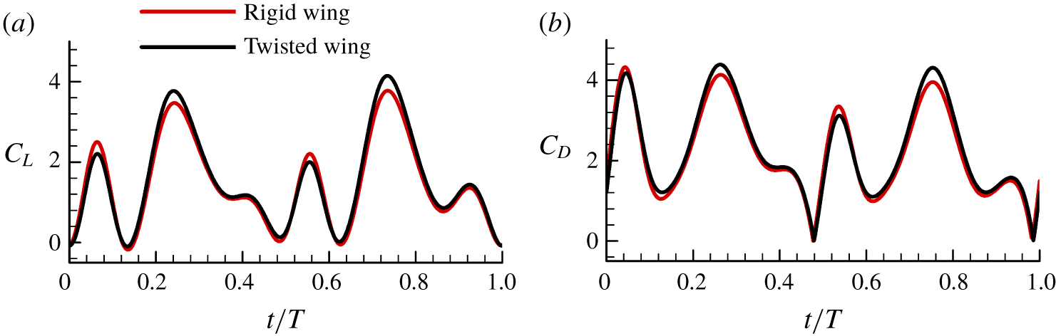
Results in appendix B (figure 23) show that the time variations of the force coefficients are similar among the eight mosquitoes. Therefore, we will only discuss the results of M1 in figure 6. As aforementioned, a mosquito wing has spanwise change in  $\unicode[STIX]{x1D6FC}$ during the flapping motion. It is of interest to look at the effect of the spanwise change in
 $\unicode[STIX]{x1D6FC}$ (wing twist) on the aerodynamic forces. We made an additional computation for M1 in which the spanwise change in
 $\unicode[STIX]{x1D6FC}$ is set to zero. The results are shown in appendix B (figure 24), compared with those with the spanwise change in
 $\unicode[STIX]{x1D6FC}$. It is seen that the spanwise change in
 $\unicode[STIX]{x1D6FC}$ has only relatively small quantitative effects on the lift and drag coefficients.
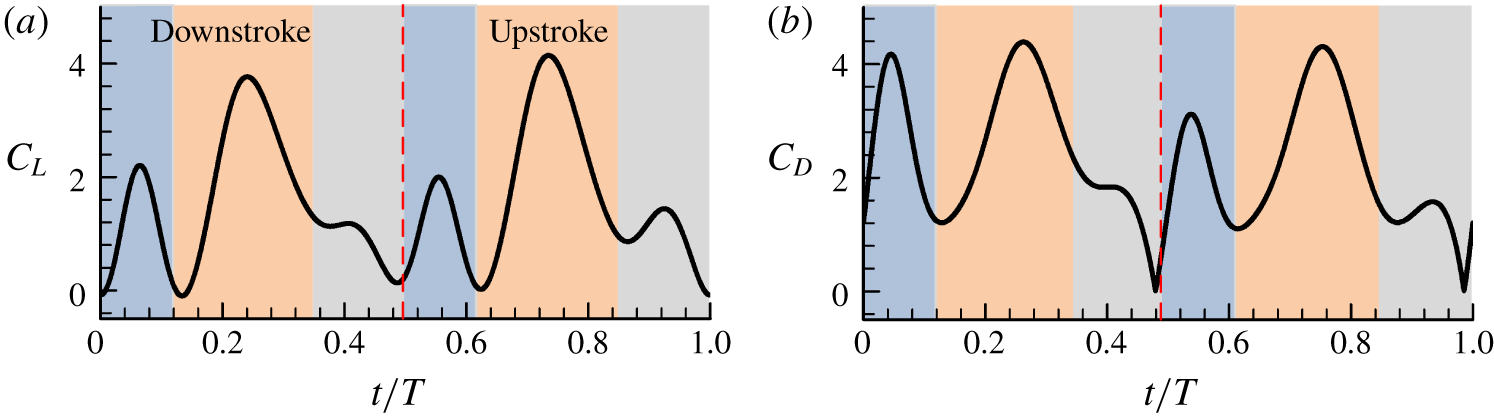
As seen from figure 6,  $C_{L}$ and
 $C_{D}$ have three peaks in a downstroke
 $(t/T=0{-}0.5)$ or upstroke
 $(t/T=0.5{-}1.0)$. For example, in the downstroke, one force peak is at the beginning of the stroke
 $(t/T\approx 0{-}0.12)$, one at the mid-portion of the stroke
 $(t/T\approx 0.12{-}0.34)$ and one near the end of the stroke
 $(t/T\approx 0.34{-}0.5)$. It is also seen that the force peaks in the beginning and in the mid-portion of the stroke, especially that in the mid-portion, are relatively large, and the force peak near the end of the stroke is relatively small. How these force peaks are produced will be analysed in the next section.
4 Aerodynamic-force production mechanisms
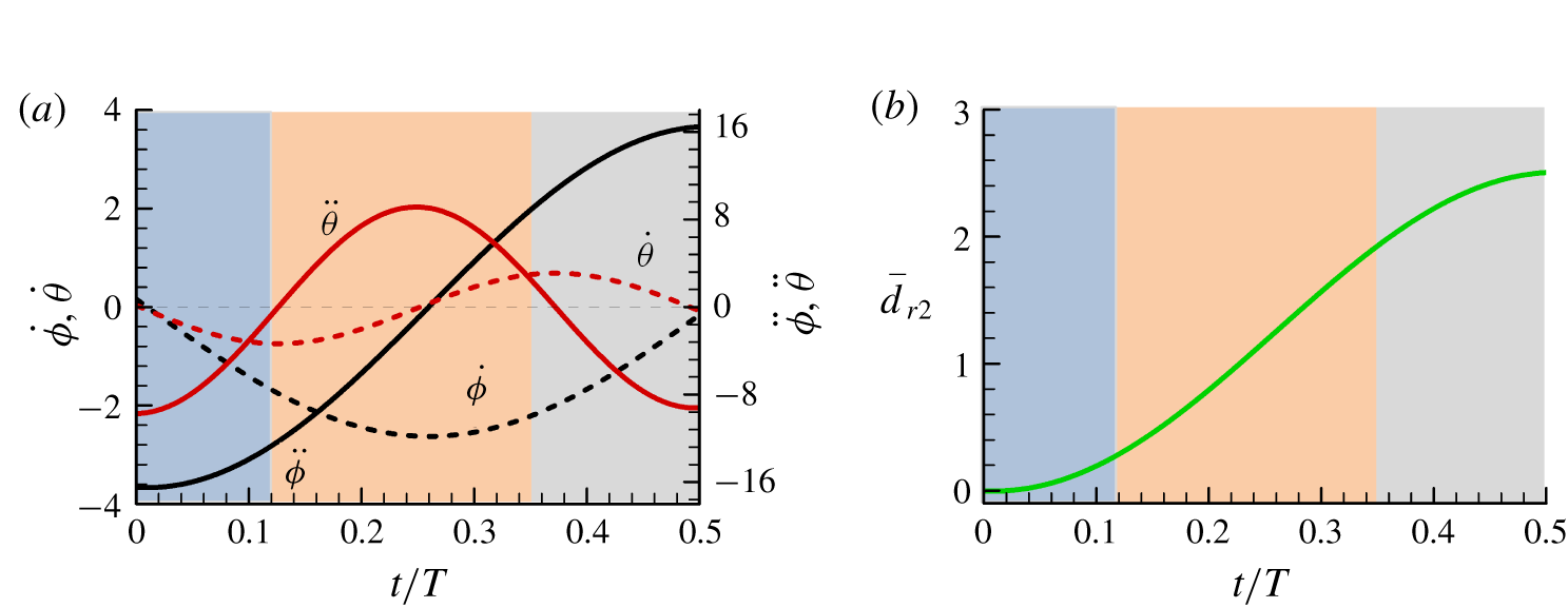
To aid in the explanation of the aerodynamic forces, we plot the time variations of the wing speed (represented by the magnitudes of  $\dot{\unicode[STIX]{x1D719}}$ and
 $\dot{\unicode[STIX]{x1D703}}$), the wing acceleration (represented by the magnitudes of
 $\ddot{\unicode[STIX]{x1D719}}$ and
 $\ddot{\unicode[STIX]{x1D703}}$) and the travel distance of the wing (represented by the travel distance of the wing section at the radius of gyration, denoted as
 $d_{r2}$; its non-dimensional value is
 $\overline{d_{r2}=d_{r2}/c}$) in a downstroke in figure 7; the corresponding values in the upstroke are similar. Since the wing motion and the aerodynamic forces are similar between the downstroke and the upstroke, hereafter we only discuss the flows in the downstroke.
The wing speed (represented by the magnitudes of  $\dot{\unicode[STIX]{x1D719}}$ and
 $\dot{\unicode[STIX]{x1D703}}$), the wing acceleration (represented by the magnitudes of
 $\ddot{\unicode[STIX]{x1D719}}$ and
 $\ddot{\unicode[STIX]{x1D703}}$) and the travel distance of the wing (
 $\overline{d}_{r2}$) in a downstroke.

It is seen that at the beginning of the stroke  $(t/T\approx 0{-}0.12)$, the magnitude of the wing acceleration (
 $\ddot{\unicode[STIX]{x1D719}}$ and
 $\ddot{\unicode[STIX]{x1D703}}$) is large (figure 7a), indicating that the added-mass effect may play an important role in this period. It is also observed that when the mid-portion of the stroke is finished, the travel distance of the wing is only approximately two wing chord lengths (see figure 7b at
 $t/T\approx 0.34$,
 $\overline{d}_{r2}\approx 2$). This means that the force peak in the mid-portion of the stroke cannot be produced by the delayed-stall mechanism, because the LEV has not completed its formation in such a short travel distance (Kim & Gharib Reference Kim and Gharib2010; Jardin, Farcy & David Reference Jardin, Farcy and David2012; Harbig et al. Reference Harbig, Sheridan and Thompson2013; Garmann & Visbal Reference Garmann and Visbal2014; Lee, Lua & Lim Reference Lee, Lua and Lim2016; Liu, Dong & Li Reference Liu, Dong and Li2016; Werner et al. Reference Werner, Chung, Wang, Liu, Cimbala, Dong and Cheng2019). These points are addressed below.
4.1 Force peak at the beginning of the downstroke or upstroke
As aforementioned, the  $C_{L}$ and
 $C_{D}$ peaks at the beginning of the downstroke or upstroke may have been produced by the added-mass effect. One way to show whether or not this is true is to compute lift and drag contributed by the added-mass force and compare them with the force peaks in this period. This is done here.
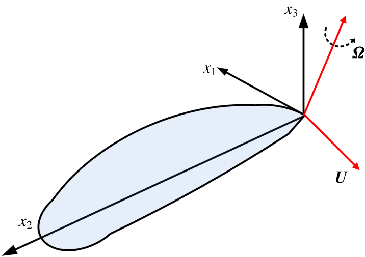
A wing in arbitrary motion in an incompressible fluid at rest at infinity.

In an inviscid, incompressible fluid, the added-mass force  $(\boldsymbol{F}_{a})$ on a body in arbitrary motion and its derivation are described in many textbooks (e.g. Newman Reference Newman1977). The major results are summarized here. Let the body be a flapping wing. The body translating at velocity
 $\boldsymbol{U}(t)$ and rotating at angular velocity
 $\unicode[STIX]{x1D734}(t)$ (figure 8). The coordinate system
 $(x_{1},x_{2},x_{3})$ is fixed on the wing (a non-inertial frame);
 $x_{2}$ is along the pitching axis of the wing,
 $x_{1}$ is along the wing-chord and
 $x_{3}$ is perpendicular to the wing surface. Let the
 $x_{1}$-,
 $x_{2}$- and
 $x_{3}$-components of
 $U(t)$ be
 $U_{1}$,
 $U_{2}$ and
 $U_{3}$, respectively, and the corresponding components of
 $\unicode[STIX]{x1D734}(t)$ be
 $U_{4}$,
 $U_{5}$ and
 $U_{6}$, respectively. The components
 $U_{1}$,
 $U_{2}$ and
 $U_{3}$ can be straightforwardly given when
 $U(t)$ is known. The components
 $U_{4}$,
 $U_{5}$ and
 $U_{6}$ are related to the flapping Euler angle as follows:
 $$\begin{eqnarray}\left[\begin{array}{@{}c@{}}U_{4}\\ U_{5}\\ U_{6}\end{array}\right]=\left[\begin{array}{@{}ccc@{}}-\text{cos}\,\unicode[STIX]{x1D703}\sin \unicode[STIX]{x1D713} & \cos \unicode[STIX]{x1D713} & 0\\ \sin \unicode[STIX]{x1D703} & 0 & 1\\ \cos \unicode[STIX]{x1D703}\cos \unicode[STIX]{x1D713} & \sin \unicode[STIX]{x1D713} & 0\end{array}\right]\left[\begin{array}{@{}c@{}}\dot{\unicode[STIX]{x1D719}}\\ \dot{\unicode[STIX]{x1D703}}\\ \dot{\unicode[STIX]{x1D713}}\end{array}\right].\end{eqnarray}$$
Here ‘ $\cdot$’ represents the time derivative. Let
 $\unicode[STIX]{x1D608}_{ij}$ (
 $i=1,2,3$;
 $j=1{-}6$) be the added-mass tensor (see appendix A for its description and its computation method). Let
 $B_{i}=-\unicode[STIX]{x1D608}_{ij}U_{j}$ (summation convention is used here and below) and
 $\boldsymbol{B}=(B_{1},B_{2},B_{3})$; then the added-mass force is (Newman Reference Newman1977)
 $$\begin{eqnarray}\boldsymbol{F}_{a}=\dot{\boldsymbol{B}}+\unicode[STIX]{x1D734}\times \boldsymbol{B}.\end{eqnarray}$$
In the special case of a body moving without rotation:  $\boldsymbol{U}\neq 0$,
 $\unicode[STIX]{x1D734}=0$ and
 $$\begin{eqnarray}\boldsymbol{F}_{a}=\dot{\boldsymbol{B}},\end{eqnarray}$$
i.e.
 $$\begin{eqnarray}\boldsymbol{F}_{a,i}=-\unicode[STIX]{x1D608}_{ij}\frac{\text{d}U_{j}}{\text{d}t}.\end{eqnarray}$$
For a given body,  $\unicode[STIX]{x1D608}_{ij}$ is determined by solving the potential flow equation, i.e. the Laplace equation of the velocity potential (see appendix A).
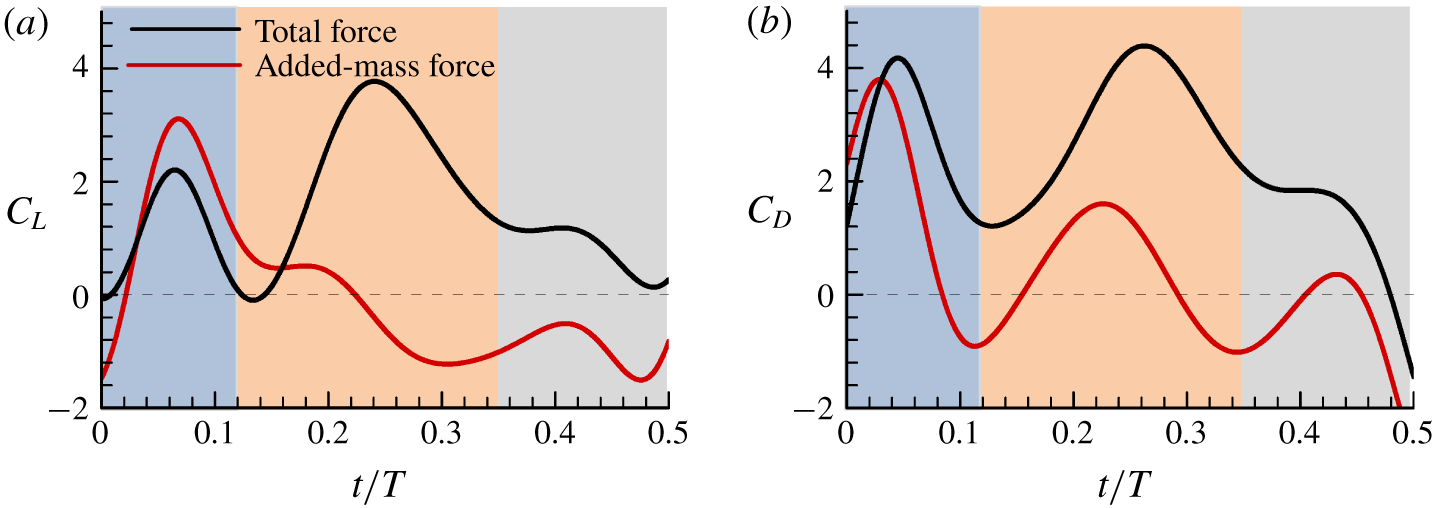
Added-mass contributions to the lift and drag.

In a viscous flow, how are the added-mass forces calculated? Howe (Reference Howe1995, Reference Howe1989) made an analysis of the force exerted on a rigid body in unsteady motion in a uniform incompressible viscous fluid. A formula was derived which expresses the force in terms of velocity of the body and vorticity and velocity of the fluid (equation (2.25) in Howe (Reference Howe1995)). The formula permits the identification of the separate effects of added mass, surface pressure induced by free vorticity and viscous skin friction. In the special case of a body moving without rotation, the formula becomes (equation (2.27) in Howe (Reference Howe1995))
 $$\begin{eqnarray}\boldsymbol{F}_{i}=-\unicode[STIX]{x1D608}_{ij}\frac{\text{d}U_{j}}{\text{d}t}+\unicode[STIX]{x1D70C}_{0}\int _{V_{f}}\unicode[STIX]{x1D735}X_{i}\boldsymbol{\cdot }(\unicode[STIX]{x1D74E}\wedge \boldsymbol{v}_{rel})\,\text{d}^{3}x+\unicode[STIX]{x1D707}_{0}\oint _{S}(\unicode[STIX]{x1D74E}\wedge \unicode[STIX]{x1D735}X_{i})\boldsymbol{\cdot }\text{d}\boldsymbol{S},\end{eqnarray}$$
where  $F_{i}$ (
 $i=1$, 2, 3) is the
 $i$th component of the force exerted on the body and
 $\unicode[STIX]{x1D608}_{ij}$ and
 $U_{j}$ have the same definitions as those in the above discussions on inviscid flow;
 $\unicode[STIX]{x1D714}$ denotes vorticity;
 $X$ denotes the velocity potential of the irrotational flow past the body (imagined to be temporarily at rest);
 $\boldsymbol{v}_{rel}=\boldsymbol{u}-\boldsymbol{U}$, where
 $\boldsymbol{u}$ is the flow velocity;
 $S$ is the body surface and
 $V_{f}$ is the flow volume which encloses all of the vorticity. The above equation shows that the force on the body is the summation of three parts. The first part is caused by the acceleration of the body, and its expression is identical to the added-mass force (4.3b) obtained by solving the potential flow of no free vorticity. The second part is due to the free vorticity in the flow. The third part is caused by the viscous skin friction. This is also true in the general case of a body moving with translation and rotation: the first term on the right-hand side of (2.25) in Howe (Reference Howe1995) is the same as the added-mass force of a potential flow (4.2). Howe’s (Reference Howe1995) results clearly show that the added-mass force of a rigid body moving in a viscous, incompressible fluid can be computed by solving a separate potential flow of no circulation. That is, we can calculate the added-mass force of the flapping wing (around which there are vortex wakes) by solving a potential flow (of the same wing motion). Since the aerodynamic force on the body consists of three parts (4.4), we called it total force, and the added-mass force is one part of the total force. As seen in (4.4),
 $F_{i}$ is the total force, the first term on the right-hand side of the equation (i.e. the added-mass term) is one part of the total force
 $F_{i}$.
Our group recently developed a code for computing the added-mass force of flapping wings, using the three-dimensional panel method (Liu & Sun Reference Liu and Sun2018); see appendix A for the validation of the code and convergence study of the panel method. Using the code we calculated the added-mass force of the mosquito wing and the results are shown in figure 9, compared with the results computed by solving the Navier–Stokes equations. It is observed that in the beginning period of the stroke  $(t/T\approx 0{-}0.12)$, the added-mass forces play a dominant role in the aerodynamic-force generation. Therefore, it can be concluded that the
 $C_{L}$ and
 $C_{D}$ peaks at the beginning of the stroke are mainly produced by the added-mass force mechanism.
It should be noted that although the added-mass force contributes positive lift in the beginning part of the stroke when the wing is in acceleration ( $t/T\approx 0{-}0.25$, figure 9a), while it contributes negative lift in the next part of the stroke
 $(t/T\approx 0.25{-}0.5)$ when the wing is in deceleration; that is, without the negative contribution of the added-mass force, the second and third lift peaks would have been larger. The time average of the added-mass lift in a stroke can be calculated from the data in figure 9(a) and the value is zero (in fact, that the time-average force due to the added-mass force is zero for a flapping wing is a well-known general result). We thus see that the added-mass force has no effect on the time-average lift and drag, but it can greatly change the time fluctuation of the aerodynamic forces.
It is observed that in the beginning period of the stroke, the added-mass force is greater than the total force in its contribution to  $C_{L}$ (
 $t/T\approx 0{-}0.12$, figure 9a). The reason for this is as follows. Contributions to the total force include the added-mass force, the surface pressure due to the free vorticity and the viscous skin friction. At the beginning of the period, the vortex wake gives a large negative contribution to the aerodynamic force, making the total force smaller than the added-mass force (see discussions on wake effect in § 5).
In the Bomphrey et al. (Reference Bomphrey, Nakata, Phillips and Walker2017) paper, it was suggested that the large  $C_{L}$ and
 $C_{D}$ peaks at the beginning of the stroke were due to the wake of the previous stroke (wake capture). But our results clearly show that the large
 $C_{L}$ and
 $C_{D}$ peaks at the beginning of the stroke are mainly produced by the added-mass effect and that their suggested explanation of the large
 $C_{L}$ and
 $C_{D}$ peaks is not correct. We will discuss why it is so in a later section (see § 5).
Lift and drag coefficients and the first moment of vorticity of the wing in the downstroke.

4.2 The force peak in the mid-portion of the downstroke or upstroke
Next we explain the  $C_{L}$ and
 $C_{D}$ peaks in the mid-portion of the downstroke or upstroke. For this purpose, we use the vortex dynamics theory on aerodynamic forces. Wu (Reference Wu1981) derived expressions relating the aerodynamic force on a body moving in an incompressible, viscous flow to the vorticity around the body. Here we explain how the
 $C_{L}$ and
 $C_{D}$ peaks in the mid-portion of the stroke are produced by using these expressions.
For a thin wing such as the insect wing, the expressions can be written as (Meng & Sun Reference Meng and Sun2015)
 $$\begin{eqnarray}\boldsymbol{F}=-\frac{\text{d}\unicode[STIX]{x1D738}}{\text{d}\unicode[STIX]{x1D70F}},\end{eqnarray}$$
where  $F$ is the non-dimensional force on the wing,
 $\unicode[STIX]{x1D70F}$ is the non-dimensional time and
 $\unicode[STIX]{x1D6FE}$ is the non-dimensional total first moment of vorticity in the fluid;
 $\unicode[STIX]{x1D6FE}$ is defined as
 $$\begin{eqnarray}\unicode[STIX]{x1D738}=\int _{V_{f}}\boldsymbol{r}\times \unicode[STIX]{x1D74E}\,\text{d}V,\end{eqnarray}$$
where  $r$ is the non-dimensional position vector,
 $\unicode[STIX]{x1D714}$ is the non-dimensional vorticity and
 $V_{f}$ is the fluid region. The total vorticity in the fluid is conserved (Wu Reference Wu1981):
 $$\begin{eqnarray}\int _{V_{f}}\unicode[STIX]{x1D74E}\,\text{d}V=0.\end{eqnarray}$$
Let  $\unicode[STIX]{x1D6FE}_{x}$,
 $\unicode[STIX]{x1D6FE}_{y}$ and
 $\unicode[STIX]{x1D6FE}_{z}$ be the
 $x$,
 $y$ and
 $z$ component of
 $\unicode[STIX]{x1D6FE}$, respectively. From (4.5) and (4.4), the lift and drag coefficients can be written as
 $$\begin{eqnarray}\displaystyle & \displaystyle C_{L}=\frac{\text{d}(-\unicode[STIX]{x1D6FE}_{z})}{\text{d}\unicode[STIX]{x1D70F}}, & \displaystyle\end{eqnarray}$$
 $$\begin{eqnarray}\displaystyle & \displaystyle C_{D}=\frac{\text{d}(-\unicode[STIX]{x1D6FE}_{x})}{\text{d}\unicode[STIX]{x1D70F}}\cos \unicode[STIX]{x1D719}+\frac{\text{d}(\unicode[STIX]{x1D6FE}_{y})}{\text{d}\unicode[STIX]{x1D70F}}\sin \unicode[STIX]{x1D719}. & \displaystyle\end{eqnarray}$$
Equations (4.5) and (4.6), or (4.8) and (4.9), state that the aerodynamic forces are proportional to the time rate of change in the total first moment of vorticity in the fluid.
(a) Iso-vorticity surface plots for the right wing in the mid-portion of the downstroke, top view (in this and other plots of iso-vorticity surfaces, the magnitude of the non-dimensional vorticity is 1.5). (b) Non-dimensional spanwise vorticity contours at different sections.

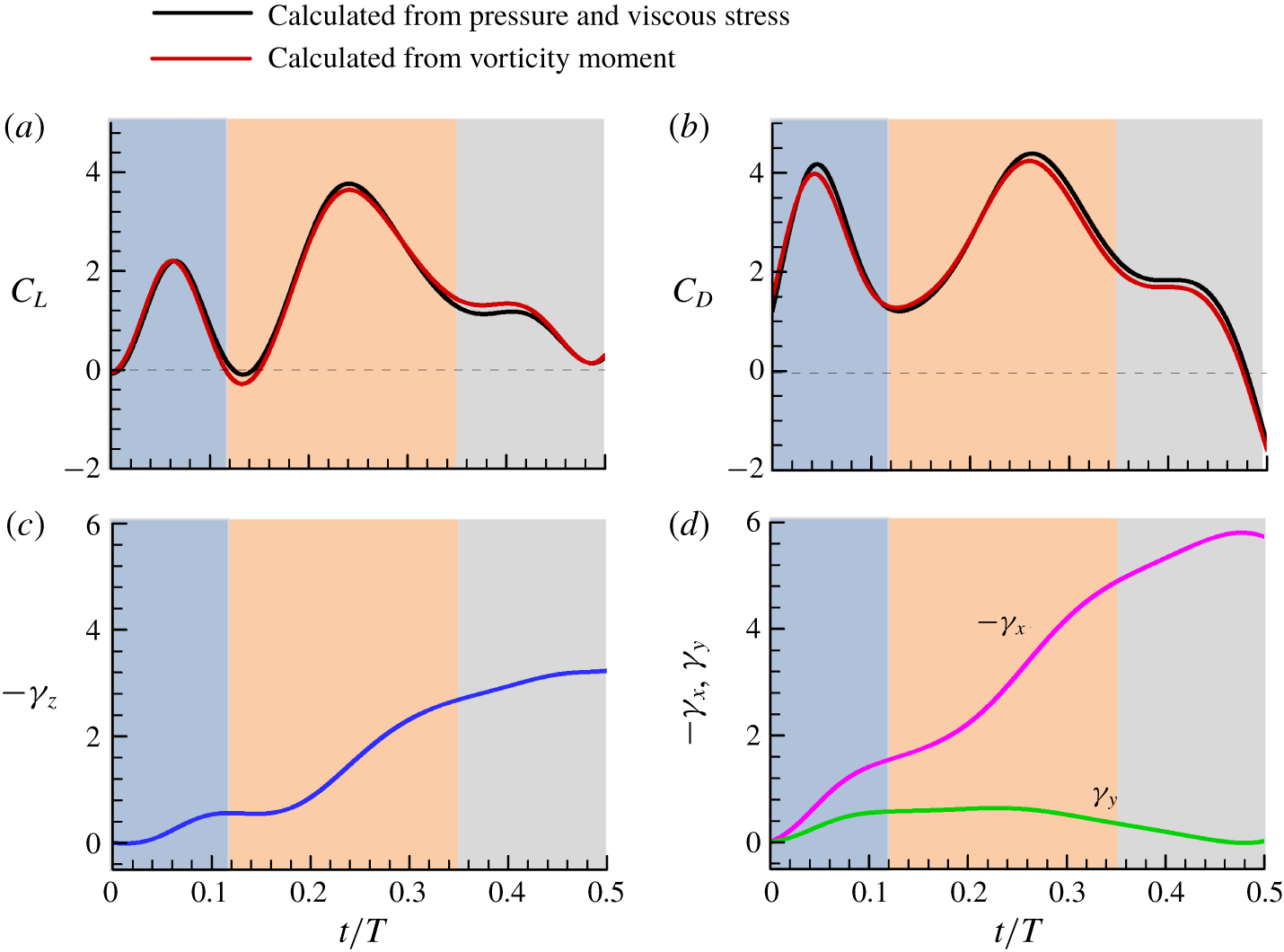
Figure 10(a,b) gives the time courses of the lift and drag coefficients calculated from the pressure and the viscous stress on the wing surface and those calculated from the total first moment of vorticity using (4.8) and (4.9). It is seen that  $C_{L}$ and
 $C_{D}$ computed from (4.8) and (4.9) are almost the same as that obtained by the usual way of integrating the pressure and viscous stress on the wing surface, as they should be. The time courses of the total first moment of vorticity
 $\unicode[STIX]{x1D6FE}_{x}$,
 $\unicode[STIX]{x1D6FE}_{y}$ and
 $\unicode[STIX]{x1D6FE}_{z}$ are also given in the figure (figure 10c,d). As seen in figure 10(c,d), the slopes of the
 $-\unicode[STIX]{x1D6FE}_{z}$ curve and
 $-\unicode[STIX]{x1D6FE}_{x}$ curve, or the time rate of change of
 $-\unicode[STIX]{x1D6FE}_{z}$ and
 $-\unicode[STIX]{x1D6FE}_{x}$, are large in the mid-portion of the stroke
 $(t/T\approx 0.12{-}0.34)$. According to (4.8), the large slope of the
 $-\unicode[STIX]{x1D6FE}_{z}$ curve gives the large
 $C_{L}$ peak in the mid-portion of the stroke. As known from the kinematic data (figure 4),
 $\unicode[STIX]{x1D719}$ is between
 $-22^{\circ }$ and
 $22^{\circ }$; thus,
 $\sin \unicode[STIX]{x1D719}$ is much less than 1 and
 $\cos \unicode[STIX]{x1D719}$ is close to 1. Therefore,
 $C_{D}$ in (4.9) is mainly determined by the time rate of change of
 $-\unicode[STIX]{x1D6FE}_{x}$. That is, the large slope of the
 $-\unicode[STIX]{x1D6FE}_{x}$ curve gives the large
 $C_{D}$ peak in the mid-portion of the stroke.
Now let us examine how the large time rates of change in  $-\unicode[STIX]{x1D6FE}_{z}$ and
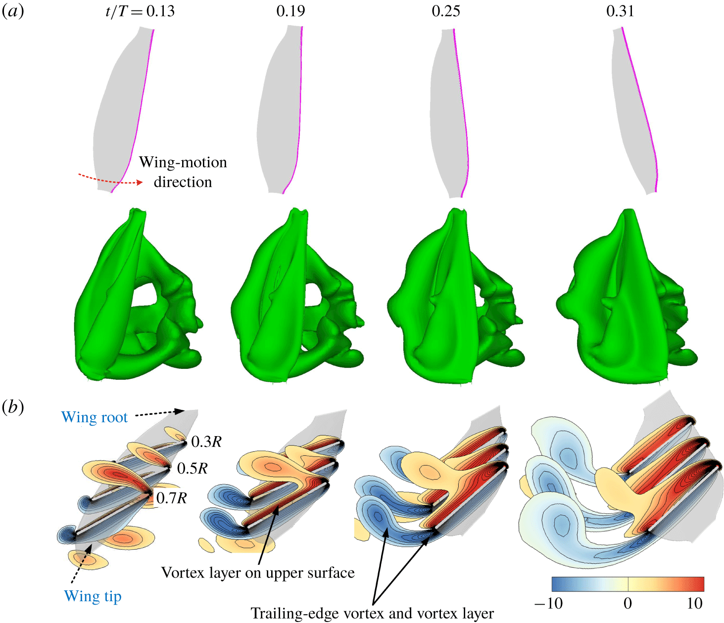
 $-\unicode[STIX]{x1D6FE}_{x}$ are produced. The non-dimensional vorticity fields at various times in the mid-portion of the stroke
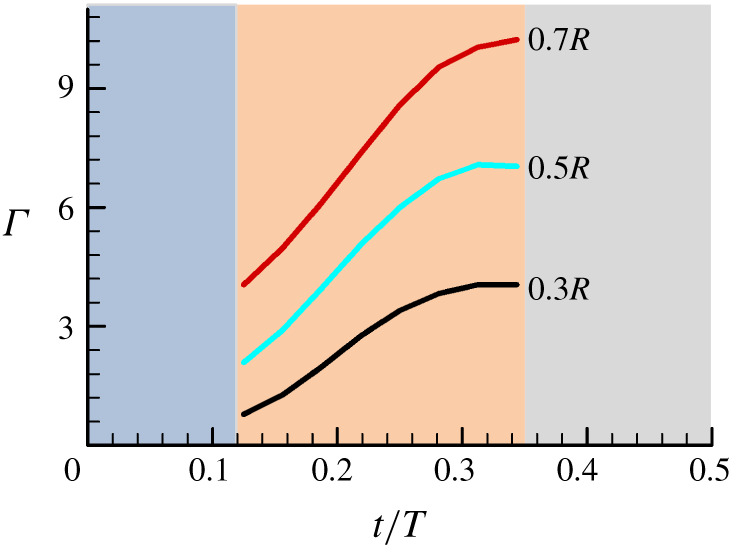
 $(t/T\approx 0.12{-}0.34)$ are plotted in figure 11, which includes the iso-vorticity surface plots and the contour plots of the spanwise component of vorticity at different spanwise locations. Here we are looking at the right wing in its downstroke (the sketch of the right wing in its downstroke can be seen in figures 3 and 11a). In figure 11(b), we look at the wing from the right side of the insect, i.e. the view frame is looking from the wing tip to the wing root. It is observed that during this period, counter clockwise (CCW) vorticity is continuously generated on the upper surface of the wing, forming a vortex layer on the upper surface (note that most of the vorticity is near the leading edge of the wing), and at the same time, clockwise (CW) vorticity is continuously generated at the trailing edge, forming a trailing-edge vortex and a vortex layer. The CCW vorticity in the vortex layer over the upper surface increases with time, and so does the CW vorticity in the trailing-edge vortex and vortex layer (figure 11b). Figure 12 gives the time variations of the non-dimensional circulation
 $(\unicode[STIX]{x1D6E4})$ of the CCW vorticity in the vortex layer over the upper surface of the wing at several spanwise locations (note that because total vorticity is conserved, the magnitude of the circulation of CW vorticity in the trailing-edge vortex and vortex layer is the same as that of the CCW vorticity). It is seen that the magnitude of the non-dimensional circulation increases with time rapidly (figure 12).
The time variations of the circulation of the CCW vorticity over the upper surface of the wing at several spanwise locations in the mid-portion of the downstroke.

(a) The time variation of the angle of attack of the wing (at  $r_{2}$ section) in the mid-portion of the downstroke. (b) The time variation of the pitching-up rate (
 $\dot{\unicode[STIX]{x1D6FC}}$) of the wing in the mid-portion of the downstroke, compared with the lift coefficient.

When there is vorticity of one sign near the leading edge and there is vorticity of the opposite sign near the trailing edge, there will be a total first moment of vorticity, comparable to two forces of equal magnitude and opposite direction separated by a distance will produce a force couple. Therefore, the rapid generation of opposite-sign vorticity at different locations of the wing will give a rapid time rate of change in the total first moment of vorticity, explaining the large time rate of changes in  $-\unicode[STIX]{x1D6FE}_{x}$ and
 $-\unicode[STIX]{x1D6FE}_{z}$ in this period.
From above, we see that for the mosquitoes, which have a very small stroke amplitude, the force peaks in the mid-portion of the stroke are produced by continuously generating large CCW vorticity on the upper surface of the wing (most of the CCW vorticity is near the leading edge of the wing) and CW vorticity at the trailing edge of the wing, in a relatively short time (or over a relatively short travelling distance of the wing). How are these large CCW and CW vorticities produced? In the mid-portion of the stroke, the wing translates at a relatively large velocity (see  $\dot{\unicode[STIX]{x1D719}}$ at
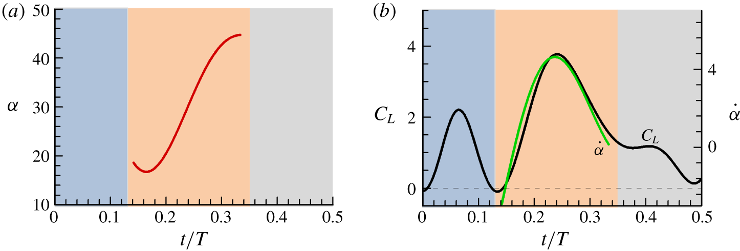
 $t/T\approx 0.12{-}0.34$ in figure 7a). At the same time, the wing pitches up rapidly:
 $\unicode[STIX]{x1D6FC}$ changes from approximately
 $16^{\circ }$ to
 $46^{\circ }$ (figure 13a). Previous studies (Dickinson et al. Reference Dickinson, Lehmann and Sane1999; Hamdani & Sun Reference Hamdani and Sun2000; Sun & Tang Reference Sun and Tang2002) have shown that when the wing is moving forward, rapid pitching up will produce large lift and drag. Figure 13(b) gives the pitching rate (
 $\dot{\unicode[STIX]{x1D6FC}}$), compared with
 $C_{L}$ in the mid-portion of the stroke. The figure (figure 13b) shows that the time course of
 $C_{L}$ is similar to that of
 $\dot{\unicode[STIX]{x1D6FC}}$, suggesting that the fast-pitching-up motion of the forward moving wing produces the large CCW vorticity and CW vorticity, and, hence, the large
 $C_{L}$ (and
 $C_{D}$). This unsteady aerodynamic-force mechanism is therefore referred to as the ‘fast-pitching-up rotation’ mechanism.
It is well known that, for a hovering insect with a relatively large stroke amplitude, the large aerodynamic forces in the mid-portion of a downstoke or upstroke is produced by the delayed-stall mechanism. In this case, at the beginning part of a stroke, the wing (at a large angle of attack) has moved (azimuthally rotated) by about  $25^{\circ }$ and the LEV has formed, and at the mid-portion of the stroke, the LEV does not detach and stall is absent, referred to as the delayed-stall mechanism (e.g. Eldredge & Jones Reference Eldredge and Jones2019). However, for the mosquitoes, the stroke amplitude is very small and the half-period of a downstroke (and an upstroke) is much shorter than the formation time of the LEV. The delayed-stall mechanism is an irrelevant feature for the aerodynamic-force production in the mosquitoes. We thus see that the aerodynamic-force production mechanism for a mosquito wing in the mid-portion of a stroke is not as suggested by Bomphrey et al. (Reference Bomphrey, Nakata, Phillips and Walker2017): being due to the LEV (the delayed-stall mechanism). The insignificance of the delayed-stall mechanism for a wing with a short stroke amplitude has been pointed out in earlier studies (Wang et al. Reference Wang, Birch and Dickinson2004; Zhu & Sun Reference Zhu and Sun2017).
4.3 The force peak near the end of the downstroke or upstroke
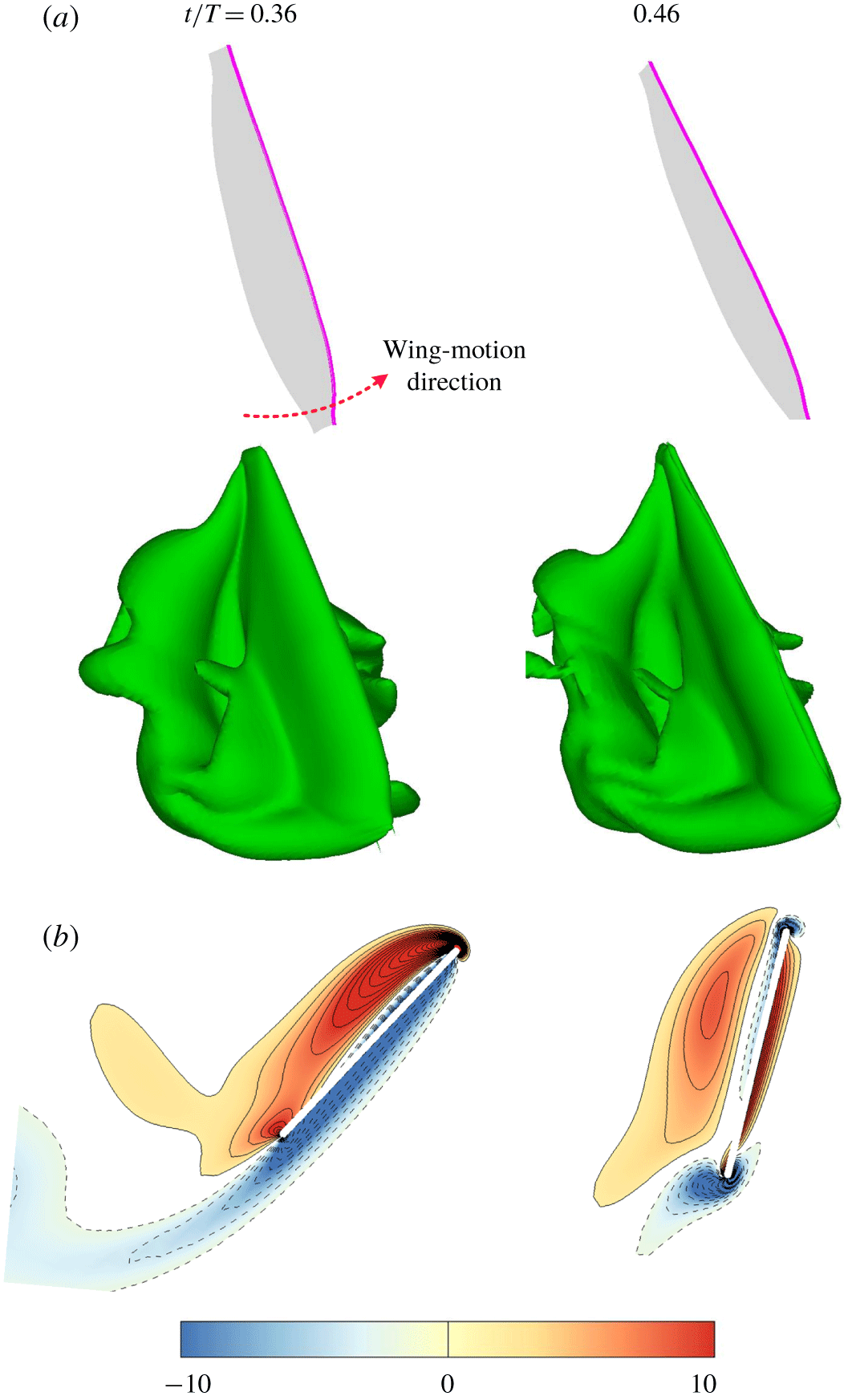
Finally, we examine the small force peaks near the end of the stroke (figure 6,  $t/T\approx 0.34{-}0.5$). The vorticity fields at various times in this period of the stroke
 $(t/T\approx 0.3{-}0.5)$ are plotted in figure 14.
Iso-vorticity surface plots (top view) (a) and non-dimensional spanwise vorticity contours at  $0.7R$ (b), near the end of the downstroke.

In this period, the wing also rapidly pitches up ( $\unicode[STIX]{x1D6FC}$ increases rapidly, as can be seen from figure 4(b),
 $t/T\approx 0.34{-}0.5$), but at the same time it is in rapid deceleration (figure 7a, the magnitudes of
 $\ddot{\unicode[STIX]{x1D719}}$ and
 $\ddot{\unicode[STIX]{x1D703}}$ are very large in
 $t/T\approx 0.34{-}0.5$). Although the pitching-up motion can produce large lift and drag, the fast deceleration has a negative effect on aerodynamic-force production (Hamdani & Sun Reference Hamdani and Sun2000). As a result, only small lift and drag peaks are produced.
The effects of wing deceleration can also be seen from the vorticity field: as seen in figure 14(b), underneath the vortex at the upper surface which contains CCW vorticity, a vortex layer of opposite vorticity (CW vorticity) is generated.
5 The effects of the wake of previous strokes
Since the mosquito wings have a very short stroke, it is expected that the wing will move near the wake it produced shortly before. Therefore, examining the effect of the wake of previous strokes on the aerodynamic-force production is of great interest. Here, we isolate the wake effect by comparing the forces of the starting downstroke (no wake effect) with those of the downstroke in the fourth wingbeat period (with the wake effect); note that the flow becomes periodic at the third wingbeat period after the flapping motion is started.
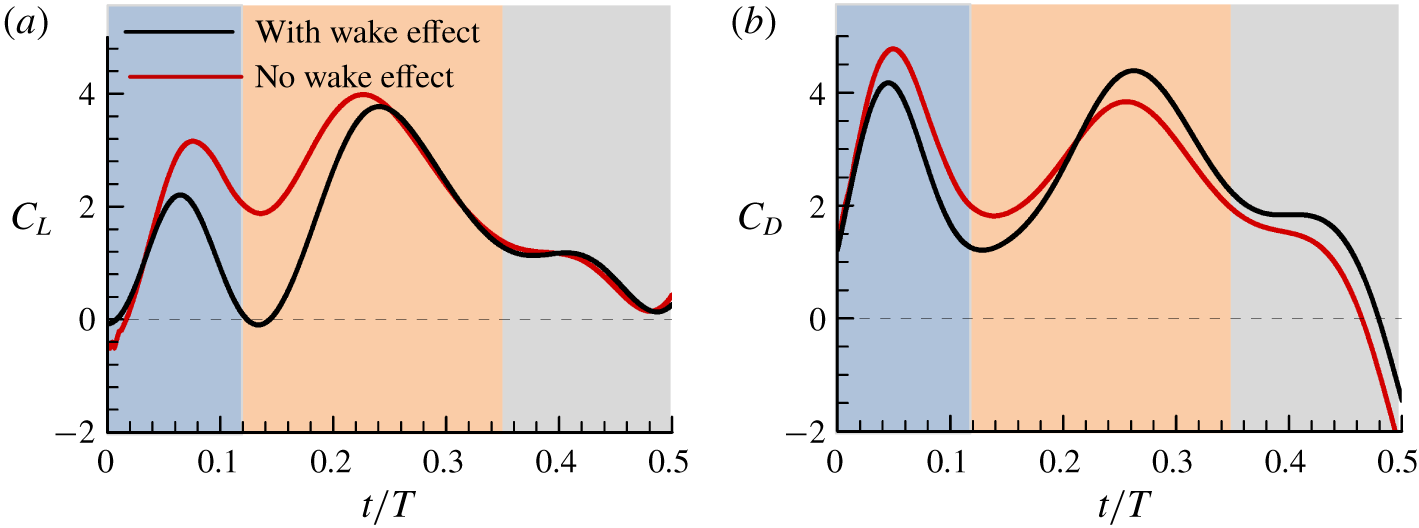
Figure 15 gives the  $C_{L}$ and
 $C_{D}$ in the first downstroke (no wake effect) compared with those of the fourth period (with wake effect). It is observed that in the first half of the stroke
 $(t/T\approx 0{-}0.25)$, the lift and drag are significantly decreased by the wake effect and, moreover, the lift reduction is larger than the drag reduction. In the second half of the stroke
 $(t/T\approx 0.25{-}0.5)$, the wake effect on the lift is small but it increases the drag. We thus see that the wake effect is detrimental: it either decreases the lift more than it decreases the drag, or it increases the drag.
Time courses of the lift and drag coefficients of the wing of M1, with and without wakes from previous strokes.

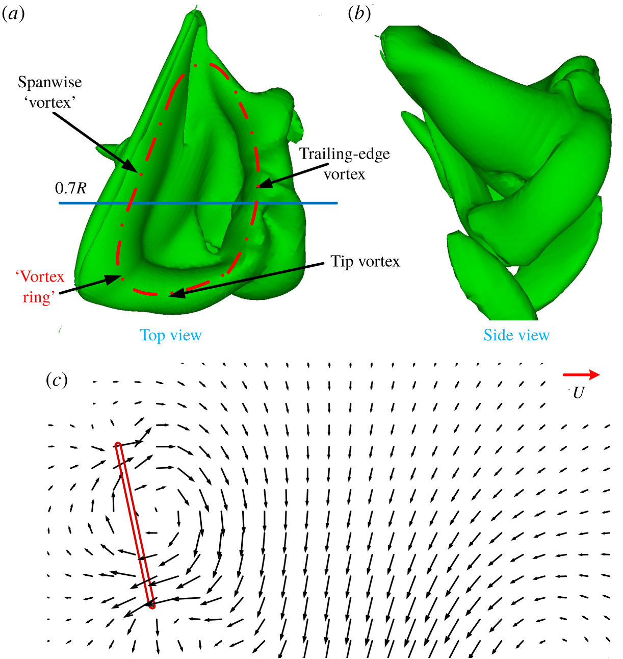
The flow field at the end of the upstroke of the third wingbeat period.

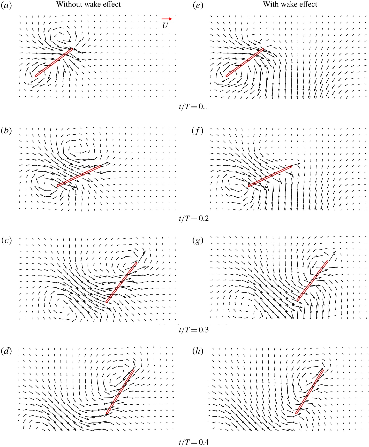
The flow field and wing section at  $0.7R$ from the wing root at various time instants during the downstroke (a–d, without wake effect; e–h, with wake effect).

Let us analyse how the above wake effects are produced. Figure 16 gives data on the flow field at the end of the upstroke of the third wingbeat period, i.e. at the start of the fourth downstroke. The flow field not far from the wing is what the wing will encounter during the beginning part of the fourth downstroke. It is observed that at this instant (the end of a stroke) there is a spanwise ‘vortex’ on the wing (the vortex layer on the upper surface of the wing), a trailing-edge vortex and a tip vortex; they form a narrow ‘vortex ring’ (figure 16a). The ‘vortex ring’ is not horizontal but is tilted to the right (figure 16b). It is well known that a vortex ring will induce a jet-like flow. Figure 16(c) gives the velocity vectors in a vertical plane at  $0.7R$ from the wing root, showing the jet-like flow produced by the ‘vortex ring’. In figure 16(c) the plate on the left represents the wing section at
 $0.7R$ from the wing root at the start of the downstroke. It is expected that during the beginning part of the fourth downstroke, the wing will move through a jet-like flow, because the flow field shown in figure 16(c) may not change much in a short time. This is further illustrated in the following. Figure 17 gives the flow field and wing section at
 $0.7R$ from the wing root at various time instants during the downstroke for both cases of the first downstroke (without wake effect) and the fourth downstroke (with wake effect). As expected, during the beginning part of the fourth downstroke (
 $t/T=0.1$ and 0.2; figure 17a,e,b,f), large downwash velocity is encountered by the wing in the case of with wake effect (e–h), while no such downwash velocity in the case of without wake effect (a–d). The downwash will reduce the effective angle of attack of the wing and, hence, reduce the resultant aerodynamic force of the wing, explaining the reductions in
 $C_{L}$ and
 $C_{D}$ in the period of
 $t/T\approx 0.02{-}0.25$ (figure 15) by the wake effect. At
 $t/T=0.3$ and 0.4 (figure 17c,g,d,h), comparing the plots on the left (without wake effect) with those on the right (with wake effect), we can see that the velocity in front of the wing is slightly reduced by the wake effect; the data indicate that the wing encounters both downward and horizontal velocities produced by the wake of the previous stroke. Since the geometrical angle of attack of the wing is large (above
 $50^{\circ }$) in this part of the stroke, the downwash velocity does not have a large effect on the effective angle of attack, but the horizontal component will increase the relative velocity. Thus, the resultant aerodynamic force will be increased. Because the wing has a very large geometrical angle of attack (i.e. the wing surface is close to be vertical), the increased resultant aerodynamic force is approximately in the horizontal direction. This explains why
 $C_{D}$ in the period of
 $t/T\approx 0.25{-}0.5$ is increased.
As aforementioned, in a previous study on the aerodynamics of mosquito flight (Bomphrey et al. Reference Bomphrey, Nakata, Phillips and Walker2017), it was suggested that the force peak in the beginning of a downstroke or upstroke (figure 6,  $t/T\approx 0{-}0.12$) was due to a trailing-edge vortex caused by the wing encountering the flow of the previous stroke (referred to as the wake capture effect). The result here shows that without the previous wake, the force peak still exists and is even bigger. Therefore, the force peak cannot be due to the wake capture effect. As analysed in § 4.1, the force peak is due to the added-mass effect.
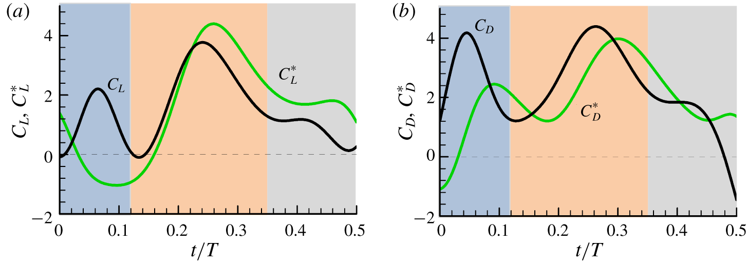
There is another way to see whether the force peak in the beginning part of a stroke is due to the added mass or due to the wake capture: to consider the total force minus the added-mass force. Subtracting the added-mass force from the total force gives the lift and drag coefficients without the added-mass contributions, denoted as  $C_{L}^{\ast }$ and
 $C_{D}^{\ast }$, respectively. They are shown in figure 18, compared with the total lift and drag. It is seen that without the added-mass contribution, the large peaks in
 $C_{L}$ and
 $C_{D}$ in the beginning part of the stroke
 $(t/T\approx 0{-}0.12)$ would not exist.
Time courses of the lift and drag coefficients of the wing of M1, with and without added-mass contribution.

6 Conclusion
It is found that a mosquitoes’ lift is produced by different aerodynamic mechanisms from those of insects with a large stroke amplitude. Those insects produce lift mainly by the leading-edge vortex which attaches to and moves with the wing, and the moving circulation of the vortex gives the lift; while mosquitoes produce lift by two highly unsteady mechanisms: the added-mass mechanism and the ‘fast-pitching-up rotation’ mechanism.
Two large lift peaks and a small one are produced in each downstroke and upstroke of the wing. The first large lift peak is at the beginning of the stroke. It is mainly the added-mass force, generated by the large acceleration of the wing at the start of the stroke. The second large lift peak is in the mid-portion of the stroke. In this period, the wing fast pitches up while moving forward, generating large-magnitude, opposite-sign vorticity at the trailing edge of the wing and near the leading edge of the wing. The rapid generation of opposite-sign vorticity at different locations of the wing results in a large time rate of change in the first moment of vorticity; hence, a large aerodynamic force. The third lift peak, which is near the end of the stroke and is small, is a result of the fast pitch-up rotation of a rapidly decelerating wing.
Acknowledgements
This research was supported by grants from the National Natural Science Foundation of China (11832004, 11672023, 11721202).
Declaration of interests
The authors report no conflict of interest.
Supplementary movies
Supplementary movies are available at https://doi.org/10.1017/jfm.2020.386.
Appendix A. Methods
A.1 Method of wing kinematics measurement
We acquired mosquitoes (Aedes aegypti) from the Institute of Zoology, Chinese Academy of Sciences. The hover flights of the mosquitoes in flight chambers were filmed using three high-speed cameras (FASTCAM Mini UX100, Photron Inc., San Diego, CA). The three cameras were orthogonally aligned and synchronized, and each of them was equipped with a 60 mm micro-Nikkor lens. A 50 W integrated red-light emitting diode (LED; luminous flux, 4000 lm; wavelength, 632 nm) was used to backlight each of the camera views and two lenses were used to make the light uniform. The camera system (figure 2a) was mounted on an optical table. The cameras were set to 5000 frames per second, a resolution of  $1280\times 1000$ pixels and a shutter speed of
 $25~\unicode[STIX]{x03BC}\text{s}$. The cameras were calibrated by using a flat glass panel with a high-accuracy black-and-white checkerboard pattern printed on it. The calibration gave the intrinsic and extrinsic parameters of each camera which determined the transform matrix of the camera (Liu & Sun Reference Liu and Sun2008; Mou, Liu & Sun Reference Mou, Liu and Sun2011). The system was manually triggered when the insect was observed to fly steadily in the filming area (approximately
 $15\times 15\times 15~\text{mm}^{3}$), which represented the intersecting field of views of the three cameras (we set the cameras to save all frames captured 0.6 s prior to the trigger point). The flight chamber is a cubic of
 $120\times 120\times 120~\text{mm}^{3}$. The experiment was conducted at relative humidity 50 %–60 % and temperature
 $26{-}27\,^{\circ }\text{C}$. It is of interest to compare our measuring method to that of Bomphrey et al. (Reference Bomphrey, Nakata, Phillips and Walker2017). In their method, the cameras have a resolution of
 $384\times 352$ pixels and the viewing volume is
 $20\times 20\times 20~\text{mm}$, and there are
 $352/20=17.6$ pixels in one mm. The wing length
 $(R)$ of their mosquitoes is approximately 2.8 mm. Therefore, over the wing length there are
 $17.6\times 2.8=49~\text{pixels}$. In our case, the cameras have a resolution of
 $1280\times 1000~\text{pixels}$ and the viewing volume is
 $15\times 15\times 15~\text{mm}$, and there are
 $1000/15=66.7$ pixels in one mm. Our mosquitoes have approximately the same wing length as theirs. Therefore, there are
 $66.7\times 2.8=187$ pixels over the wing length. That is, the resolution of our method is
 $187/49=3.8$ times as good as that of theirs. On the other hand, they used eight cameras and we used three, i.e. their cameras number is
 $8/3=2.7$ times as many as ours. Thus, for a set of cameras, our measuring error is much smaller than theirs, while they used more sets of cameras for reducing the errors. Based on the above discussion, we can say that our method is at least equivalent to that of Bomphrey et al. (Reference Bomphrey, Nakata, Phillips and Walker2017).
After the filming, the three-dimensional body and wing kinematics can be extracted from the filmed data. The method used for the kinematics reconstruction was developed in our previous works (Liu & Sun Reference Liu and Sun2008; Mou et al. Reference Mou, Liu and Sun2011; Meng & Sun Reference Meng and Sun2016) and is briefly described here. The body and wings were represented by models: the model of a wing was a flat-plate wing having the outline obtained by scanning the cut-off wing (figure 2c) and that of the body was two lines perpendicular to each other, which were the lines connecting the head and the end of the abdomen and the line connecting the two wing roots (figure 2b). An interactive graphic user interface was developed using Matlab (Matlab v. 7.1, The Mathworks, Inc., Natick, MA, USA) to extract the body and wing positions from the three frames recorded by the cameras. The positions and orientations of the models of the body and wings were adjusted manually until the best overlap between a model image and the displayed frame was achieved in three views, and at this point the positions and orientations of these models were taken as the positions and orientations of the body and the wings. In the above method, the model of the wing was a rigid flat-plate. But because mosquito wings are slender, during the flapping motion they have spanwise change in pitch change (twisted along the wing length; as can be observed from the films). We dealt with this problem by making the following changes to the above method. The model of the wing was no longer a rigid flat-plate wing, but a plate wing that could have linear spanwise change in pitch along its length (we found that with the linear pitch change added in the method, a good match between a model image and the displayed frame could be achieved). The procedure of matching the model’s projection with the wing picture was changed to the following: at each time step, an initial pitch change was also assumed, and it was adjusted until a best match between the wing model and the wing picture was obtained.
The method of measurement of the morphological data can be found in Mou et al. (Reference Mou, Liu and Sun2011). The data included: the total mass  $(m)$ of the mosquito; the wing length
 $(R)$; the area of one wing
 $(S)$; the radius of the second moment of the wing area, or radius of gyration
 $(r_{2})$; the distance between the two wing roots
 $(l_{r})$.
A.2 Flow solution method and grid tests
To study the aerodynamic forces on an insect, in principle, we need to compute the flow fields around the wings and the body. But at hovering, the aerodynamic force of the body is negligibly small compared to that of the wings because the body does not move. Furthermore, it has been shown that the wings and the body do not interact aerodynamically, neither do the contralateral wings (Aono et al. Reference Aono, Liang and Liu2008; Yu & Sun Reference Yu and Sun2009; Liang & Sun Reference Liang and Sun2013). Therefore, in the present study, only one wing is simulated.
The solution method is the same as that used by our group in many previous studies (Sun & Tang Reference Sun and Tang2002; Sun & Yu Reference Sun and Yu2006; Du & Sun Reference Du and Sun2010) and only an outline of the method is given here. The algorithm is based on the method of artificial compressibility and it was developed by Rogers et al. (Reference Rogers, Kwak and Kiris1991). In the method, the time derivatives of the momentum equations are differenced using a second-order, three-point backward difference formula. To solve the time discretized momentum equations for a divergence free velocity at a new time level, a pseudo-time level is introduced into the equations and a pseudo-time derivative of pressure divided by an artificial compressibility constant is introduced into the continuity equation. The resulting system of equations is iterated in pseudo-time until the pseudo-time derivative of pressure approaches zero; thus, the divergence of the velocity at the new time level approaches zero. The derivatives of the viscous fluxes in the momentum equation are approximated using second-order central differences. For the derivatives of convective fluxes, upwind differencing based on the flux-difference splitting technique is used. A third-order upwind differencing is used at the interior points and a second-order upwind differencing is used at points next to boundaries. Details of this algorithm can be found in the paper by Rogers et al. (Reference Rogers, Kwak and Kiris1991). For far-field boundary conditions, the pressure is set equal to the static pressure of the air at infinity and the velocity is extrapolated from the interior; on the wing surface, impermeable wall and non-slip conditions are applied and the pressure is obtained through the normal component of the momentum equation written in the moving grid system.
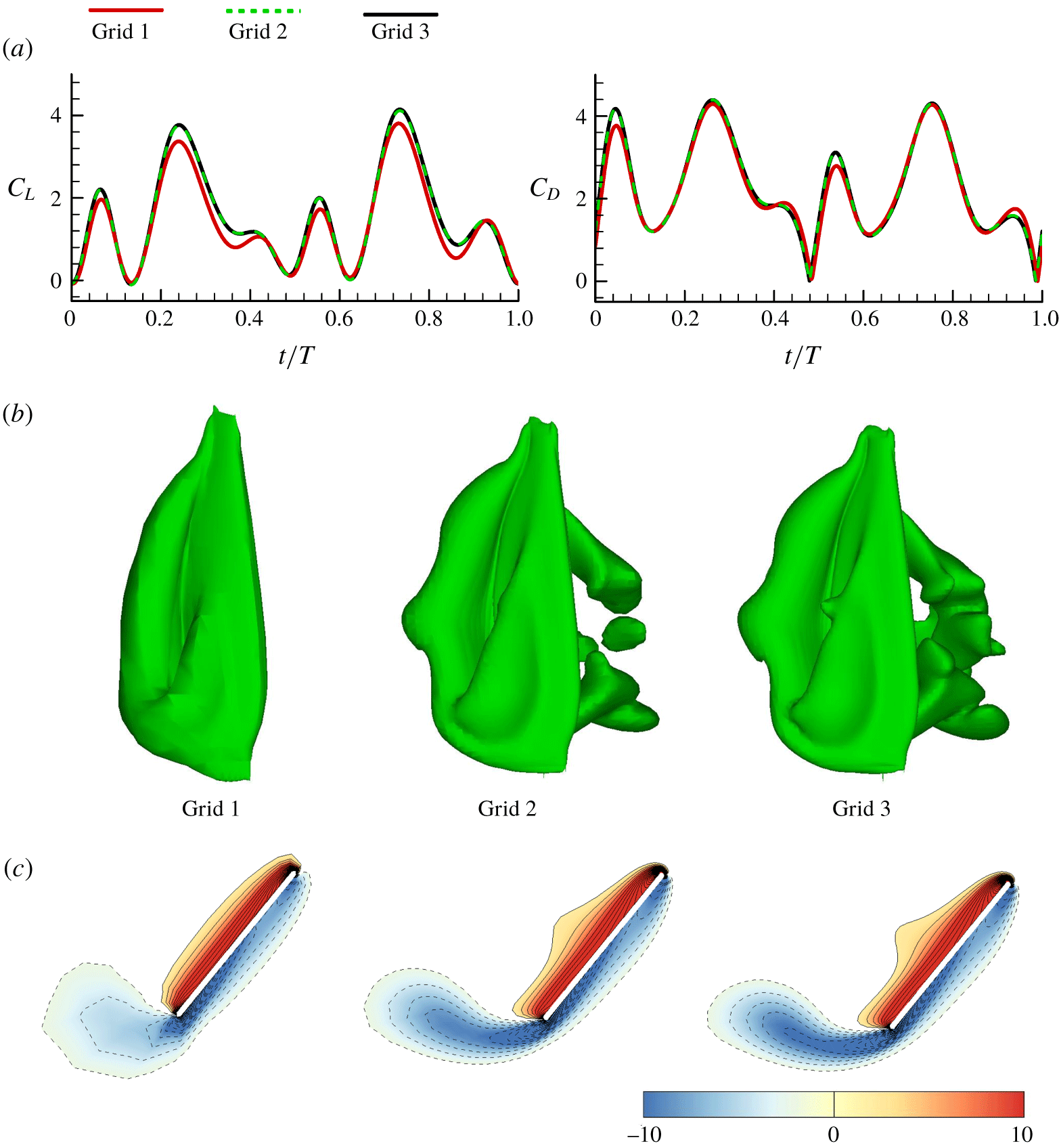
Test simulations were conducted to ensure that the computed results were independent of artificial numerical variables, such as the grid size, domain size and so on. In the test simulations, the kinematics of wing-flapping motion was taken from our measured data of mosquito M1. First, three grids were considered. Grid 1:  $28\times 28\times 36$ in the normal direction, around the wing section, and in the spanwise direction, respectively; Grid 2:
 $56\times 56\times 73$; Grid 3:
 $113\times 113\times 147$. The outer boundary was set at 20 chord lengths from the wing. Portions of the third grid
 $(113\times 113\times 147)$ are shown in figure 5. This grid was used in the computations of the present study, and its spacings and distributions are described as follows. In the normal direction, the first layer thickness was
 $0.001c$ and going away from the wing surface, the grid spacing increased by a ratio of about 1.06. Around a wing section, on the semi-circle at the leading (or trailing) edge, the grid spacing was
 $0.0039c$ and away from the leading (or trailing) edge, the spacing increased by a ratio of about 1.18. In the spanwise direction, the grid spacing can be clearly seen from figure 5. The time step was
 $T/480$. At each time step sub-iterations were carried out until both the maximum divergence of velocity at any point and the maximum residual at any point were less than
 $10^{-5}$. For each time step, about 38 sub-iterations were required. Figure 19 shows
 $C_{L}$ and
 $C_{D}$ in one cycle, computed with the above three grids, and also shown are the contours of the non-dimensional spanwise component of vorticity at the half-wing length at
 $t/T=0.25$ and the corresponding iso-vorticity surface. The following are observed: the first grid refinement produces some changes in the forces and the vorticity plots; however, after the second grid refinement, the discrepancies are considerably reduced.
Lift and drag coefficients and flow fields in a flapping cycle computed with different grids.

Next, the effect of domain size was considered. A larger computational domain was obtained by adding more grid points to the outside of grid 3 (the distance between the outer boundary and the wing was increased from  $20c$ to
 $40c$). The calculated results showed that there was no need to put the outer boundary further than that of grid 3. Finally, the effect of the time step value was considered and the results were as follows. It was shown that a numerical solution effectively independent of the time step was achieved if the time step
 $\unicode[STIX]{x0394}t\leqslant T/480$. Based on the above tests, grid 3
 $(113\times 113\times 147)$ and a time step of
 $\unicode[STIX]{x0394}t=T/480$ are used for the simulations.
A.3 Calculation method of added-mass force and its validation
As shown in Newman (Reference Newman1977) and many other textbooks on fluid mechanics, the added mass is obtained by solving for six velocity potentials. Each of them satisfies the Laplace equation, and represents the velocity potential due to the body motion with unit velocity in the  $j$th mode:
 $j=1,2,3$ correspond to unit translational velocities in the
 $x_{1}$,
 $x_{2}$ and
 $x_{3}$ directions (figure 8), respectively, and
 $j=4,5,6$ correspond to unit rotational velocities about the
 $x_{1}$,
 $x_{2}$ and
 $x_{3}$ axes (figure 8), respectively. The authors recently developed a code for solving the velocity potentials and computing the added-mass force (Liu & Sun Reference Liu and Sun2018). The code was based on a three-dimension panel method.
The code was validated by comparing it with the analytical results of a sphere with radius  $a$ and a spheroid with semi-axes
 $a$ and
 $b$ and
 $b/a=10$. For the sphere,
 $\unicode[STIX]{x1D608}_{11}\;(=\unicode[STIX]{x1D608}_{22}=\unicode[STIX]{x1D608}_{33})$ are non-zero and other
 $\unicode[STIX]{x1D608}_{ij}$ are zero; therefore, only
 $\unicode[STIX]{x1D608}_{11}$ is considered in the comparison. For the spheroid,
 $\unicode[STIX]{x1D608}_{11}$,
 $\unicode[STIX]{x1D608}_{22}\;(=\unicode[STIX]{x1D608}_{33})$ and
 $\unicode[STIX]{x1D608}_{55}\;(=\unicode[STIX]{x1D608}_{66})$ are non-aero and other
 $\unicode[STIX]{x1D608}_{ij}$ are zero; therefore, only
 $\unicode[STIX]{x1D608}_{11}$,
 $\unicode[STIX]{x1D608}_{22}$ and
 $\unicode[STIX]{x1D608}_{55}$ are considered in the comparison. The elements of the added-mass tensor are non-dimensionalized in the comparison. For the sphere,
 $\unicode[STIX]{x1D608}_{11}^{\ast }=\unicode[STIX]{x1D608}_{11}/\unicode[STIX]{x1D70C}a^{3}$ (symbol ‘
 $^{\ast }$’ denotes non-dimensional value); for the spheroid,
 $\unicode[STIX]{x1D608}_{11}^{\ast }=3\unicode[STIX]{x1D608}_{11}/4\unicode[STIX]{x03C0}\unicode[STIX]{x1D70C}ab^{2}$,
 $\unicode[STIX]{x1D608}_{22}^{\ast }=3\unicode[STIX]{x1D608}_{22}/4\unicode[STIX]{x03C0}\unicode[STIX]{x1D70C}ab^{2}$ and
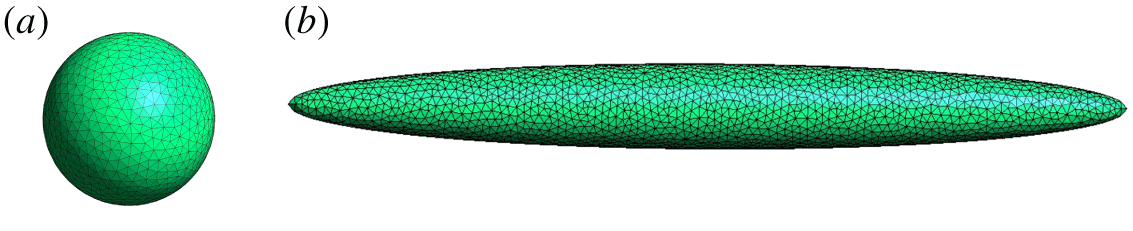
 $\unicode[STIX]{x1D608}_{55}^{\ast }=15\unicode[STIX]{x1D608}_{55}/4\unicode[STIX]{x03C0}\unicode[STIX]{x1D70C}ab^{2}(a^{2}+b^{2})$. Figure 20 shows the panels on the surface of bodies. Table 3 gives the comparison between the panel-method results and the analytical results; the analytical result of the sphere is from Newman (Reference Newman1977) and that of the spheroid is from Sahin, Crane & Waston (Reference Sahin, Crane and Waston1993). As seen in table 3, for the sphere, as the number of panels is about
 $10^{4}$, the result of the panel method is different from the analytical one by only 0.03 % and, for the spheroid, as the panel number is about
 $2\times 10^{4}$, the corresponding differences are less than 0.12 %. This validates our panel-method code.
A sphere and a spheroid with surface panels.

Comparison between the panel-method results and the analytical results.

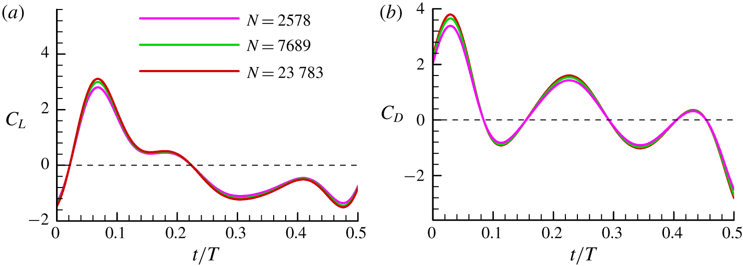
Before applying the code to the calculation of the added mass of the flapping wing, test simulations were conducted to ensure that the computed results were independent of the number of panels  $(N)$. In the test simulations, the wing flapping was taken from the measured data of mosquito M1. Three panel numbers were considered,
 $N=2578$, 7689 and 23 783. Figure 21 shows the
 $C_{L}$ and
 $C_{D}$ due to the added-mass force computed using the above three panel numbers. It is observed that the first refinement of the panel size produces some changes in the
 $C_{L}$ and
 $C_{D}$; however, after the second refinement, little discrepancy is observed. Based on these tests, in our calculations of the added-mass force,
 $N=23\,783$ is used.
Lift and drag coefficients due to the added-mass force, computed with different panel numbers.

Measured data of wing kinematics for all eight mosquitoes.

Computed lift  $(C_{L})$ and drag
 $(C_{D})$ coefficients for all eight individuals.

Appendix B. Measured and computed results for all eight individuals
Measured data of wing-flapping motion (figure 22) and computed lift and drag (figure 23) are shown for all eight individuals. Results of the effect of wing twist on aerodynamic forces are also shown here (figure 24).
Lift  $(C_{L})$ and drag
 $(C_{D})$ coefficients computed with a rigid wing and twisted wing.