2. Problem formulation and governing equations

We consider a static equilibrium that consists of a straight homogeneous magnetic tube. The equilibrium magnetic field is $\boldsymbol{B}_{0}=B_{0}\boldsymbol{n}$ , where $B_{0}$ is a constant and $\boldsymbol{n}$ is the unit vector parallel to the tube axis. The equilibrium density ${\it\rho}_{0}$ is constant inside and outside the tube. Hence, in cylindrical coordinates $r,{\it\varphi},z$ , with the $z$ -axis coinciding with the tube axis, the density is given by

(2.1) $$\begin{eqnarray}{\it\rho}_{0}=\left\{\begin{array}{@{}ll@{}}{\it\rho}_{0i}, & r<a,\\ {\it\rho}_{0e}, & r>a,\end{array}\right.\end{eqnarray}$$

where $a$ is the tube radius. To describe the plasma motion we use the ideal magnetohydrodynamic equations in the zero-beta approximation,

(2.2a ) $$\begin{eqnarray}\displaystyle & \displaystyle \frac{\partial \bar{{\it\rho}}}{\partial t}+\boldsymbol{{\rm\nabla}}\boldsymbol{\cdot }(\bar{{\it\rho}}\boldsymbol{V})=0, & \displaystyle\end{eqnarray}$$

(2.2b ) $$\begin{eqnarray}\displaystyle & \displaystyle \frac{\partial \boldsymbol{V}}{\partial t}+(\boldsymbol{V}\boldsymbol{\cdot }\boldsymbol{{\rm\nabla}})\boldsymbol{V}=\frac{1}{{\it\mu}_{0}\bar{{\it\rho}}}(\boldsymbol{{\rm\nabla}}\times \boldsymbol{B})\times \boldsymbol{B}, & \displaystyle\end{eqnarray}$$

(2.2c ) $$\begin{eqnarray}\displaystyle & \displaystyle \frac{\partial \boldsymbol{B}}{\partial t}=\boldsymbol{{\rm\nabla}}\times (\boldsymbol{V}\times \boldsymbol{B}). & \displaystyle\end{eqnarray}$$

$\boldsymbol{V}=(V_{r},V_{{\it\varphi}},V_{z})$

$\boldsymbol{B}=(B_{r},B_{{\it\varphi}},B_{z})$

$\bar{{\it\rho}}$

${\it\mu}_{0}$

(2.3a,b ) $$\begin{eqnarray}\tilde{{\it\rho}}=\bar{{\it\rho}}-{\it\rho}_{0},\quad \tilde{\boldsymbol{B}}=\boldsymbol{B}-\boldsymbol{B}_{0}.\end{eqnarray}$$

We do not introduce the velocity perturbation because there is no equilibrium flow. In what follows, we use the dimensionless variables

(2.4a−c ) $$\begin{eqnarray}{\it\rho}=\frac{\tilde{{\it\rho}}}{{\it\rho}_{0}},\quad \boldsymbol{v}=\frac{\boldsymbol{V}}{V_{A}},\quad \boldsymbol{b}=\frac{\tilde{\boldsymbol{B}}}{\boldsymbol{B}_{0}},\end{eqnarray}$$

where $V_{A}=B_{0}/\sqrt{{\it\mu}_{0}{\it\rho}_{0}}$ is the Alfvén speed. Then we rewrite the system of (2.2) as

(2.5a ) $$\begin{eqnarray}\frac{1}{V_{A}}\frac{\partial {\it\rho}}{\partial t}+\boldsymbol{{\rm\nabla}}\boldsymbol{\cdot }\boldsymbol{v}=-\boldsymbol{{\rm\nabla}}\boldsymbol{\cdot }({\it\rho}\boldsymbol{v}),\end{eqnarray}$$

(2.5b ) $$\begin{eqnarray}\displaystyle \frac{1}{V_{A}}\frac{\partial \boldsymbol{v}}{\partial t}-(\boldsymbol{{\rm\nabla}}\times \boldsymbol{b})\times \boldsymbol{n} & = & \displaystyle -(\boldsymbol{v}\boldsymbol{\cdot }\boldsymbol{{\rm\nabla}})\boldsymbol{v}+(\boldsymbol{{\rm\nabla}}\times \boldsymbol{b})\times \boldsymbol{b}-{\it\rho}(\boldsymbol{{\rm\nabla}}\times \boldsymbol{b})\times \boldsymbol{n}\nonumber\\ \displaystyle & & \displaystyle -\,{\it\rho}(\boldsymbol{{\rm\nabla}}\times \boldsymbol{b})\times \boldsymbol{b}+{\it\rho}^{2}(\boldsymbol{{\rm\nabla}}\times \boldsymbol{b})\times \boldsymbol{n},\end{eqnarray}$$

(2.5c ) $$\begin{eqnarray}\frac{1}{V_{A}}\frac{\partial \boldsymbol{b}}{\partial t}-\boldsymbol{{\rm\nabla}}\times (\boldsymbol{v}\times \boldsymbol{n})=\boldsymbol{{\rm\nabla}}\times (\boldsymbol{v}\times \boldsymbol{b}).\end{eqnarray}$$

When deriving these equations we have only kept the quadratic and cubic nonlinear terms.

The system of (2.5) has to be supplemented with the conditions at the tube boundary. We write the equation of the perturbed tube boundary as $r=a[1+{\it\eta}(t,z)]$ . The function ${\it\eta}$ is independent of ${\it\varphi}$ because we only consider sausage, i.e. axisymmetric, perturbations. The kinematic boundary condition is written as

(2.6) $$\begin{eqnarray}V_{r}=a\frac{\partial {\it\eta}}{\partial t}+a\boldsymbol{V}\boldsymbol{\cdot }\boldsymbol{{\rm\nabla}}{\it\eta}\quad \text{at}\;r=a(1+{\it\eta}).\end{eqnarray}$$

Note that, in fact, this equation contains two boundary conditions because it is valid for the velocity both inside as well as outside the magnetic tube.

The second boundary condition is the dynamic one stating that the magnetic pressure must be the same at the two sides of the tube boundary. It reads

(2.7) $$\begin{eqnarray}\boldsymbol{B}_{i}^{2}=\boldsymbol{B}_{e}^{2}\quad \text{at}\;r=a(1+{\it\eta}),\end{eqnarray}$$

where the subscripts ‘ $i$ ’ and ‘ $e$ ’ indicate that a quantity is calculated inside or outside the tube, respectively. Using the dimensionless variables, we rewrite the boundary conditions (2.6) and (2.7) as

(2.8a ) $$\begin{eqnarray}\displaystyle & \displaystyle \frac{v_{r}}{a}=\frac{1}{V_{A}}\frac{\partial {\it\eta}}{\partial t}+\boldsymbol{v}\boldsymbol{\cdot }\boldsymbol{{\rm\nabla}}{\it\eta}\quad \text{at}\;r=a(1+{\it\eta}), & \displaystyle\end{eqnarray}$$

(2.8b ) $$\begin{eqnarray}\displaystyle & \displaystyle \boldsymbol{b}_{i}\boldsymbol{\cdot }(2\boldsymbol{n}+\boldsymbol{b}_{i})=\boldsymbol{b}_{e}\boldsymbol{\cdot }(2\boldsymbol{n}+\boldsymbol{b}_{e})\quad \text{at}\;r=a(1+{\it\eta}). & \displaystyle\end{eqnarray}$$

3. Derivation of equation for the radial velocity

We start the derivation of the equation for the radial velocity by writing the system of (2.5) and the boundary conditions (2.8) in components. As we have already stated, we only consider axisymmetric plasma motions, so all the variables are independent of ${\it\varphi}$ . In addition, we eliminate torsional motions, so $v_{{\it\varphi}}=b_{{\it\varphi}}=0$ . Then we obtain the equations

(3.1a ) $$\begin{eqnarray}\displaystyle & \displaystyle \frac{1}{V_{A}}\frac{\partial {\it\rho}}{\partial t}+\frac{1}{r}\frac{\partial (rv_{r})}{\partial r}+\frac{\partial v_{z}}{\partial z}=-\frac{1}{r}\frac{\partial (r{\it\rho}v_{r})}{\partial r}-\frac{\partial ({\it\rho}v_{z})}{\partial z}\equiv F_{1}, & \displaystyle\end{eqnarray}$$

(3.1b ) $$\begin{eqnarray}\displaystyle & \displaystyle \frac{1}{V_{A}}\frac{\partial v_{r}}{\partial t}-\frac{\partial b_{r}}{\partial z}+\frac{\partial b_{z}}{\partial r}=(1-{\it\rho})(b_{z}-{\it\rho})\left(\frac{\partial b_{r}}{\partial z}-\frac{\partial b_{z}}{\partial r}\right)-v_{r}\frac{\partial v_{r}}{\partial r}-v_{z}\frac{\partial v_{r}}{\partial z}\equiv F_{2},\qquad & \displaystyle\end{eqnarray}$$

(3.1c ) $$\begin{eqnarray}\displaystyle & \displaystyle \frac{1}{V_{A}}\frac{\partial v_{z}}{\partial t}=(1-{\it\rho})b_{r}\left(\frac{\partial b_{z}}{\partial r}-\frac{\partial b_{r}}{\partial z}\right)-v_{r}\frac{\partial v_{z}}{\partial r}-v_{z}\frac{\partial v_{z}}{\partial z}\equiv F_{3}, & \displaystyle\end{eqnarray}$$

(3.1d ) $$\begin{eqnarray}\displaystyle & \displaystyle \frac{1}{V_{A}}\frac{\partial b_{r}}{\partial t}-\frac{\partial v_{r}}{\partial z}=-\frac{\partial }{\partial z}(v_{z}b_{r}-v_{r}b_{z})\equiv F_{4}, & \displaystyle\end{eqnarray}$$

(3.1e ) $$\begin{eqnarray}\displaystyle & \displaystyle \frac{1}{V_{A}}\frac{\partial b_{z}}{\partial t}+\frac{1}{r}\frac{\partial (rv_{r})}{\partial r}=\frac{1}{r}\frac{\partial }{\partial r}r(v_{z}b_{r}-v_{r}b_{z})\equiv F_{5}. & \displaystyle\end{eqnarray}$$

${\it\epsilon}\ll 1$

$v_{z}=O({\it\epsilon}^{2})$

(3.2a ) $$\begin{eqnarray}\displaystyle & \displaystyle \frac{v_{r}}{a}=\frac{1}{V_{A}}\frac{\partial {\it\eta}}{\partial t}+v_{z}\frac{\partial {\it\eta}}{\partial z}\quad \text{at}\;r=a(1+{\it\eta}), & \displaystyle\end{eqnarray}$$

(3.2b ) $$\begin{eqnarray}\displaystyle & \displaystyle \unicode[STIX]{x27E6}2b_{z}+b_{r}^{2}+b_{z}^{2}\unicode[STIX]{x27E7}=0\quad \text{at}\;r=a(1+{\it\eta}), & \displaystyle\end{eqnarray}$$

$f(r)$

(3.3) $$\begin{eqnarray}\displaystyle \unicode[STIX]{x27E6}\,f(r)\unicode[STIX]{x27E7}=\lim _{{\it\varepsilon}\rightarrow +0}[\,f(a+a{\it\eta}+{\it\varepsilon})-f(a+a{\it\eta}-{\it\varepsilon})]. & & \displaystyle\end{eqnarray}$$

Differentiating equation (3.1b ) with respect to time and using (3.1d ) and (3.1e ) we derive the equation

(3.4) $$\begin{eqnarray}\frac{1}{V_{A}^{2}}\frac{\partial ^{2}v_{r}}{\partial t^{2}}-{\it\Delta}_{2}v_{r}=\frac{1}{V_{A}}\frac{\partial F_{2}}{\partial t}+\frac{\partial F_{4}}{\partial z}-\frac{\partial F_{5}}{\partial r},\end{eqnarray}$$

where

(3.5) $$\begin{eqnarray}{\it\Delta}_{2}={\rm\nabla}^{2}-\frac{1}{r^{2}}.\end{eqnarray}$$

Introducing the operator $I=\int \text{d}t$ we obtain from (3.1)

(3.6a ) $$\begin{eqnarray}\displaystyle & \displaystyle {\it\rho}=-V_{A}I\left(\frac{1}{r}\frac{\partial }{\partial r}rv_{r}+\frac{\partial v_{z}}{\partial z}\right)-V_{A}I\left(\frac{1}{r}\frac{\partial }{\partial r}{\it\rho}rv_{r}+\frac{\partial {\it\rho}v_{z}}{\partial z}\right), & \displaystyle\end{eqnarray}$$

(3.6b ) $$\begin{eqnarray}\displaystyle & \displaystyle v_{z}=-V_{A}I\left(v_{r}\frac{\partial v_{z}}{\partial r}+v_{z}\frac{\partial v_{z}}{\partial z}\right)-V_{A}I(1-{\it\rho})b_{r}\left(\frac{\partial b_{r}}{\partial z}-\frac{\partial b_{z}}{\partial r}\right), & \displaystyle\end{eqnarray}$$

(3.6c ) $$\begin{eqnarray}\displaystyle & \displaystyle b_{r}=V_{A}I\frac{\partial v_{r}}{\partial z}-V_{A}I\frac{\partial }{\partial z}(v_{z}b_{r}-v_{r}b_{z}), & \displaystyle\end{eqnarray}$$

(3.6d ) $$\begin{eqnarray}\displaystyle & \displaystyle b_{z}=-\frac{V_{A}}{r}I\frac{\partial }{\partial r}rv_{r}+\frac{V_{A}}{r}I\frac{\partial }{\partial r}r(v_{z}b_{r}-v_{r}b_{z}). & \displaystyle\end{eqnarray}$$

(3.7a ) $$\begin{eqnarray}\displaystyle & \displaystyle {\it\rho}=V_{A}^{2}I\frac{1}{r}\frac{\partial }{\partial r}\left(v_{r}I\frac{\partial (rv_{r})}{\partial r}\right)-\frac{V_{A}}{r}I\frac{\partial (rv_{r})}{\partial r}+V_{A}^{4}I^{2}\frac{\partial }{\partial z}\left(I\frac{\partial v_{r}}{\partial z}\right)I{\it\Delta}_{2}v_{r}+O({\it\epsilon}^{3}),\quad & \displaystyle\end{eqnarray}$$

(3.7b ) $$\begin{eqnarray}\displaystyle & \displaystyle v_{z}=-V_{A}^{3}I\left(I\frac{\partial v_{r}}{\partial z}\right)I{\it\Delta}_{2}v_{r}+O({\it\epsilon}^{3}), & \displaystyle\end{eqnarray}$$

(3.7c ) $$\begin{eqnarray}\displaystyle & \displaystyle b_{r}=V_{A}I\frac{\partial v_{r}}{\partial z}-V_{A}^{2}I\frac{\partial }{\partial z}\left(\frac{v_{r}}{r}I\frac{\partial (rv_{r})}{\partial r}\right)+O({\it\epsilon}^{3}), & \displaystyle\end{eqnarray}$$

(3.7d ) $$\begin{eqnarray}\displaystyle b_{z} & = & \displaystyle -\frac{V_{A}}{r}I\frac{\partial (rv_{r})}{\partial r}+\frac{V_{A}^{2}}{r}I\frac{\partial }{\partial r}\left(v_{r}I\frac{\partial (rv_{r})}{\partial r}\right)\nonumber\\ \displaystyle & & \displaystyle -\,\frac{V_{A}^{3}}{r}I\frac{\partial }{\partial r}r\left[V_{A}^{2}\left(I\frac{\partial v_{r}}{\partial z}\right)I\left(I\frac{\partial v_{r}}{\partial z}\right)I{\it\Delta}_{2}v_{r}+\frac{v_{r}}{r}I\frac{\partial }{\partial r}\left(v_{r}I\frac{\partial (rv_{r})}{\partial r}\right)\right]+O({\it\epsilon}^{4}).\nonumber\\ \displaystyle & & \displaystyle\end{eqnarray}$$

Using (3.7), we can express the right-hand side of equation (3.4) in terms of $v_{r}$ :

(3.8) $$\begin{eqnarray}\frac{1}{V_{A}^{2}}\frac{\partial ^{2}v_{r}}{\partial t^{2}}-{\it\Delta}_{2}v_{r}=P+Q+O({\it\epsilon}^{4}),\end{eqnarray}$$

where $P$ contains quadratic and $Q$ cubic terms. These quantities are given by

(3.9) $$\begin{eqnarray}P=-V_{A}{\it\Delta}_{2}\left(\frac{v_{r}}{r}I\frac{\partial (rv_{r})}{\partial r}\right)-V_{A}\frac{\partial }{\partial r}(v_{r}I{\it\Delta}_{2}v_{r}),\end{eqnarray}$$

(3.10) $$\begin{eqnarray}\displaystyle Q\! & = & \displaystyle \!V_{A}^{2}{\it\Delta}_{2}\left[V_{A}^{2}\left(I\frac{\partial v_{r}}{\partial z}\right)I\left(I\frac{\partial v_{r}}{\partial z}\right)I{\it\Delta}_{2}v_{r}+\frac{v_{r}}{r}I\frac{\partial }{\partial r}\left(v_{r}I\frac{\partial (rv_{r})}{\partial r}\right)\right]\nonumber\\ \displaystyle & & \displaystyle +\,V_{A}^{4}\left\{\left[I\left(I\frac{\partial v_{r}}{\partial z}\right)I{\it\Delta}_{2}v_{r}\right]\frac{\partial }{\partial z}-\left[\frac{\partial }{\partial z}I\left(I\frac{\partial v_{r}}{\partial z}\right)I{\it\Delta}_{2}v_{r}\right]\right\}I{\it\Delta}_{2}v_{r}\nonumber\\ \displaystyle & & \displaystyle -\,V_{A}^{4}({\it\Delta}_{2}v_{r})I^{2}\frac{\partial }{\partial z}\left(I\frac{\partial v_{r}}{\partial z}\right)I{\it\Delta}_{2}v_{r}+V_{A}^{2}\frac{\partial v_{r}}{\partial z}\left(I\frac{\partial v_{r}}{\partial z}\right)I{\it\Delta}_{2}v_{r}\nonumber\\ \displaystyle & & \displaystyle +\,\frac{\partial }{\partial r}\left[v_{r}^{2}\frac{\partial v_{r}}{\partial r}+V_{A}^{2}v_{r}I{\it\Delta}_{2}\left(\frac{v_{r}}{r}I\frac{\partial (rv_{r})}{\partial r}\right)\right].\end{eqnarray}$$

To derive (3.9) and (3.10) we have used the expressions for $F_{2}$ , $F_{4}$ and $F_{5}$ obtained in appendix A.

It is shown in appendix B that the boundary conditions (3.2) can be transformed to

(3.11) $$\begin{eqnarray}\displaystyle & & \displaystyle \left.\unicode[STIX]{x27E6}V_{A}v_{r}+V_{A}^{2}\frac{\partial v_{r}}{\partial r}Iv_{r}+V_{A}^{3}\left(\frac{\partial v_{r}}{\partial r}I\frac{\partial v_{r}}{\partial r}Iv_{r}+\frac{1}{2}\frac{\partial ^{2}v_{r}}{\partial r^{2}}(Iv_{r})^{2}\right)\right.\nonumber\\ \displaystyle & & \displaystyle \quad +\left.V_{A}^{5}\left(I\frac{\partial v_{r}}{\partial r}\right)I\left(I\frac{\partial v_{r}}{\partial z}\right)I{\it\Delta}_{2}v_{r}\right.\unicode[STIX]{x27E7}=O({\it\epsilon}^{4}),\end{eqnarray}$$

(3.12) $$\begin{eqnarray}\displaystyle & & \displaystyle \left.\unicode[STIX]{x27E6}\frac{2V_{A}}{a}I\frac{\partial (rv_{r})}{\partial r}-V_{A}^{2}\left(I\frac{\partial v_{r}}{\partial z}\right)^{2}-\frac{V_{A}^{2}}{a^{2}}\left(I\frac{\partial (rv_{r})}{\partial r}\right)^{2}-\frac{2V_{A}^{2}}{a}I\frac{\partial }{\partial r}\left(v_{r}I\frac{\partial (rv_{r})}{\partial r}\right)\right.\nonumber\\ \displaystyle & & \displaystyle \quad +\,\frac{2V_{A}^{2}}{a}I(Iv_{r})\frac{\partial }{\partial r}r\frac{\partial v_{r}}{\partial r}+\frac{V_{A}^{3}}{a}\left\{I(Iv_{r})^{2}\frac{\partial }{\partial r}r\frac{\partial ^{2}v_{r}}{\partial r^{2}}+2I\left(I\frac{\partial v_{r}}{\partial r}Iv_{r}\right)\frac{\partial }{\partial r}r\frac{\partial v_{r}}{\partial r}\right.\nonumber\\ \displaystyle & & \displaystyle \quad -\,2I\left(\frac{\partial ^{2}v_{r}}{\partial r^{2}}Iv_{r}\right)I\frac{\partial (rv_{r})}{\partial r}-2I\frac{\partial v_{r}}{\partial r}I\left((Iv_{r})\frac{\partial }{\partial r}r\frac{\partial v_{r}}{\partial r}\right)-2I\left(\frac{\partial v_{r}}{\partial r}Iv_{r}\right)I\frac{\partial ^{2}(rv_{r})}{\partial r^{2}}\nonumber\\ \displaystyle & & \displaystyle \quad -\,2Iv_{r}I\left((Iv_{r})\frac{\partial ^{2}}{\partial r^{2}}r\frac{\partial v_{r}}{\partial r}\right)-2\left(I\frac{\partial v_{r}}{\partial z}\right)\left(aI\frac{\partial ^{2}v_{r}}{\partial r\partial z}Iv_{r}-I\frac{\partial }{\partial z}v_{r}I\frac{\partial (rv_{r})}{\partial r}\right)\nonumber\\ \displaystyle & & \displaystyle \quad +\,2I\frac{\partial }{\partial r}r\left[V_{A}^{2}\left(I\frac{\partial v_{r}}{\partial z}\right)I\left(I\frac{\partial v_{r}}{\partial z}\right)I{\it\Delta}_{2}v_{r}+\frac{v_{r}}{a}I\frac{\partial }{\partial r}\left(v_{r}I\frac{\partial (rv_{r})}{\partial r}\right)\right]\nonumber\\ \displaystyle & & \displaystyle \quad -\left.\left.\frac{2}{a}\left(I\frac{\partial (rv_{r})}{\partial r}\right)\left(I(Iv_{r})\frac{\partial }{\partial r}r\frac{\partial v_{r}}{\partial r}-I\frac{\partial }{\partial r}v_{r}I\frac{\partial (rv_{r})}{\partial r}\right)\right\}\vphantom{\frac{V_{A}^{2}}{a^{2}}\left(I\frac{\partial (rv_{r})}{\partial r}\right)^{2}}\!\right.\unicode[STIX]{x27E7}=O({\it\epsilon}^{4}).\end{eqnarray}$$

$r=a$

4. Linear fast sausage waves

In this section we briefly recall the properties of linear fast sausage waves. These waves are described by the linearized equation (3.8), i.e. (3.8) with the right-hand side equal to zero, and the linearized boundary conditions (3.11) and (3.12). We take $v_{r}=\bar{v}_{r}(r)\exp (\text{i}kz-\text{i}{\it\omega}t)$ . Then the linearized equation (3.8) reduces to

(4.1) $$\begin{eqnarray}\frac{\text{d}^{2}\bar{v}_{r}}{\text{d}r^{2}}+\frac{1}{r}\frac{\text{d}\bar{v}_{r}}{\text{d}r}-\left({\it\lambda}^{2}+\frac{1}{r^{2}}\right)\bar{v}_{r}=0,\quad {\it\lambda}^{2}=k^{2}-\frac{{\it\omega}^{2}}{V_{A}^{2}}.\end{eqnarray}$$

The linearized boundary conditions (3.11) and (3.12) take the form

(4.2a,b ) $$\begin{eqnarray}\unicode[STIX]{x27E6}V_{A}\bar{v}_{r}\unicode[STIX]{x27E7}=0,\quad \left.\unicode[STIX]{x27E6}V_{A}\frac{\partial (r\bar{v}_{r})}{\partial r}\right.\unicode[STIX]{x27E7}=0\quad \text{at}\;r=a.\end{eqnarray}$$

Equation (4.1) is the Bessel equation when ${\it\lambda}^{2}<0$ and the modified Bessel equation when ${\it\lambda}^{2}>0$ . We only consider trapped waves characterized by the property that the wave amplitude decays fast enough with the distance from the tube so that the total wave energy is finite. If we assume that ${\it\lambda}_{e}^{2}<0$ , then the solution to (4.1) is expressed in terms of Bessel functions that decay as $r^{-1/2}$ when $r$ increases. The density of the wave energy is proportional to the wave amplitude squared, so it would decay as $r^{-1}$ . As a result, the total wave energy is infinite. On the basis of this analysis we conclude that, in trapped waves, ${\it\lambda}_{e}^{2}>0$ . In that case, with the accuracy up to a multiplicative constant, the solution to (4.1) decaying as $r\rightarrow \infty$ is equal to $\text{K}_{1}({\it\lambda}_{e}r)$ , where $\text{K}_{1}$ is the modified Bessel function of the second kind (McDonald function). It is shown by, e.g. Edwin & Roberts (Reference Edwin and Roberts1983) that ${\it\omega}/k>V_{Ai}$ for fast sausage waves, so ${\it\lambda}_{i}^{2}<0$ . Again with the accuracy up to a multiplicative constant, the solution to (4.1) with ${\it\lambda}_{i}^{2}<0$ that is regular at $r=0$ is $\text{J}_{1}(|{\it\lambda}_{i}|r)$ , where $\text{J}_{1}$ is the Bessel function of the first kind. Taking $\bar{v}_{r}$ proportional to $\text{J}_{1}(|{\it\lambda}_{i}|r)$ for $r<a$ , and to $\text{K}_{1}({\it\lambda}_{e}r)$ for $r>a$ , and substituting in the boundary conditions (4.2) gives the dispersion equation

(4.3) $$\begin{eqnarray}\frac{\text{J}_{1}(a|{\it\lambda}_{i}|)}{|{\it\lambda}_{i}|\text{J}_{0}(a|{\it\lambda}_{i}|)}+\frac{\text{K}_{1}(a{\it\lambda}_{e})}{{\it\lambda}_{e}\text{K}_{0}(a{\it\lambda}_{e})}=0.\end{eqnarray}$$

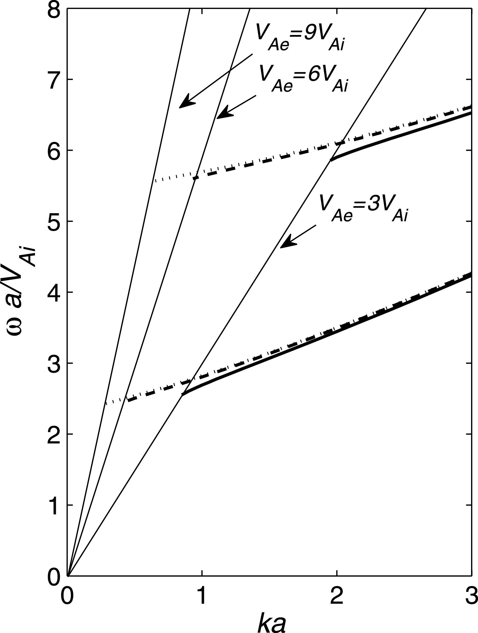
For each $k>0$ this equation describes a countable set of wave modes propagating in the positive $z$ -direction ( ${\it\omega}>0$ ). Each mode is characterized by the number of nodes of the function $\bar{v}_{r}(r)$ inside the tube. An important property of fast sausage modes is that each mode only exists as a trapped wave if $k>k_{c}$ , where $k_{c}$ increases with the increase in the node number. In figure 1 the dispersion curves for the mode fundamental in the radial direction, and for the first overtone are shown.

Figure 1.

The dependence of the wave frequency on the wavenumber. The thin straight lines show the dependence of the external Alfvén frequency ${\it\omega}_{A}$ on the wavenumber for various values of $V_{Ae}/V_{Ai}$ shown in the figure. The equation of these curves is ${\it\omega}a/V_{Ai}=kaV_{Ae}/V_{Ai}$ . The lower thick curves correspond to the mode fundamental in the radial direction (the only node of $v_{r}$ in the radial direction is at the tube axis). The upper thick curves correspond to the first overtone in the radial direction (two nodes of $v_{r}$ in the radial direction). The solid, dashed and dotted lines correspond to $V_{Ae}/V_{Ai}=3,6$ , and $9$ . Note that ${\it\omega}(k_{c})={\it\omega}_{Ae}=K_{c}V_{Ae}$ .

5. Derivation of the NLS equation

To derive the NLS equation we introduce two stretching spatial variables as well as two stretching temporal variables,

(5.1a−d ) $$\begin{eqnarray}Z_{1}={\it\epsilon}z,\quad T_{1}={\it\epsilon}t,\quad Z_{2}={\it\epsilon}^{2}z,\quad T_{2}={\it\epsilon}^{2}t,\end{eqnarray}$$

where ${\it\epsilon}\ll 1$ . Then we search for the solution to (3.8) with the boundary conditions (3.11) and (3.12) in the form

(5.2) $$\begin{eqnarray}v_{r}={\it\epsilon}v_{r1}+{\it\epsilon}^{2}v_{2r}+{\it\epsilon}^{3}v_{3r}+\text{c.c.},\end{eqnarray}$$

where

(5.3) $$\begin{eqnarray}\displaystyle & v_{r1}=A(Z_{1},T_{1},Z_{2},T_{2}){\it\Lambda}(r)\text{e}^{\text{i}(kz-{\it\omega}t)}, & \displaystyle\end{eqnarray}$$

(5.4) $$\begin{eqnarray}\displaystyle & {\it\Lambda}(r)=\left\{\begin{array}{@{}ll@{}}\text{J}_{1}(r|{\it\lambda}_{i}|), & r<a,\\ \displaystyle \frac{V_{Ai}\text{J}_{1}(a|{\it\lambda}_{i}|)}{V_{Ae}\text{K}_{1}(a{\it\lambda}_{e})}\text{K}_{1}(r{\it\lambda}_{e}), & r>a,\end{array}\right. & \displaystyle\end{eqnarray}$$

$v_{2r}$ and $v_{3r}$ depend on $r,z,t,Z_{1},T_{1},Z_{2}$ and $T_{2}$ , and c.c. indicates a complex conjugate.

The method used to obtain the NLS equation is the following. We substitute the expansion (5.2) in (3.8) and the boundary conditions (3.11) and (3.12). Then, we collect terms of the order of ${\it\epsilon}$ , ${\it\epsilon}^{2}$ , and ${\it\epsilon}^{3}$ . The first-order approximation recovers the linear theory. The solution of the second-order approximation only exists when a compatibility condition is satisfied. This condition is that the coefficient function $A$ in the expansion (5.3) depends not on $Z_{1}$ and $T_{1}$ separately, but on their combination $Z_{1}-V_{g}T_{1}$ , where $V_{g}$ is the group velocity. Thereafter we obtain the expression for $v_{2r}$ . The NLS equation is obtained as the compatibility condition for the third-order approximation.

In accordance with this we substitute the operator

(5.5) $$\begin{eqnarray}\frac{\partial }{\partial t}+{\it\epsilon}\frac{\partial }{\partial T_{1}}+{\it\epsilon}^{2}\frac{\partial }{\partial T_{2}}\end{eqnarray}$$

for the operator $\partial /\partial t$ , and the operator

(5.6) $$\begin{eqnarray}\frac{\partial }{\partial z}+{\it\epsilon}\frac{\partial }{\partial Z_{1}}+{\it\epsilon}^{2}\frac{\partial }{\partial Z_{2}}\end{eqnarray}$$

for the operator $\partial /\partial z$ . To find what operator must by substituted for the operator $I$ we use the fact that the identity $g=If$ is equivalent to $f=\partial g/\partial t$ . We look for the expression for $g$ in the form $g=g_{0}+{\it\epsilon}g_{1}+{\it\epsilon}^{2}g_{2}$ . Then, substituting the operator given by (5.5) for $\partial /\partial t$ , we obtain

(5.7) $$\begin{eqnarray}f=\frac{\partial g_{0}}{\partial t}+{\it\epsilon}\left(\frac{\partial g_{1}}{\partial t}+\frac{\partial g_{0}}{\partial T_{1}}\right)+{\it\epsilon}^{2}\left(\frac{\partial g_{2}}{\partial t}+\frac{\partial g_{1}}{\partial T_{1}}+\frac{\partial g_{0}}{\partial T_{2}}\right)+O({\it\epsilon}^{3}).\end{eqnarray}$$

Collecting terms of the order of unity we obtain from this equation

(5.8) $$\begin{eqnarray}g_{0}=If.\end{eqnarray}$$

Collecting terms on the order of ${\it\epsilon}$ in (5.7) and using (5.8) yields

(5.9) $$\begin{eqnarray}g_{1}=-I\frac{\partial g_{0}}{\partial T_{1}}=-I^{2}\frac{\partial f}{\partial T_{1}}.\end{eqnarray}$$

Finally, collecting terms of the order of ${\it\epsilon}^{2}$ in (5.7) and using (5.8) and (5.9) we arrive at

(5.10) $$\begin{eqnarray}g_{2}=-I\frac{\partial g_{1}}{\partial T_{1}}-I\frac{\partial g_{0}}{\partial T_{2}}=-I^{2}\frac{\partial f}{\partial T_{2}}+I^{3}\frac{\partial f}{\partial T_{1}^{2}}.\end{eqnarray}$$

It follows from (5.8), (5.9), and (5.10) that we must substitute the operator

(5.11) $$\begin{eqnarray}I-{\it\epsilon}I^{2}\frac{\partial }{\partial T_{1}}-{\it\epsilon}^{2}\left(I^{2}\frac{\partial }{\partial T_{2}}-I^{3}\frac{\partial }{\partial T_{1}^{2}}\right)\end{eqnarray}$$

for the operator $I$ . When performing the calculation below, we keep in mind that the operators defined by (5.5), (5.6) and (5.11) are substituted for the operators $\partial /\partial t$ , $\partial /\partial z$ and $I$ , respectively.

Now we substitute the expansion given by (5.2) in (3.8), and in the boundary conditions (3.11) and (3.12) and collect terms of various orders. In the first-order approximation, we collect terms of the order of ${\it\epsilon}$ . As a result, we recover the linear theory and obtain for $v_{r}$ the expression given by the term proportional to ${\it\epsilon}$ in (5.2).

5.1. Second-order approximation

In the second-order approximation we collect terms of the order of ${\it\epsilon}^{2}$ in (3.8). As a result, we obtain the equation

(5.12) $$\begin{eqnarray}\displaystyle \left(\frac{1}{V_{A}^{2}}\frac{\partial ^{2}}{\partial t^{2}}-{\it\Delta}_{2}\right)v_{2r} & = & \displaystyle 2\text{i}\left(\frac{{\it\omega}}{V_{A}^{2}}\frac{\partial A}{\partial T_{1}}+k\frac{\partial A}{\partial Z_{1}}\right){\it\Lambda}_{e}^{\text{i}(kz-{\it\omega}t)}\nonumber\\ \displaystyle & & \displaystyle -\,{\it\Delta}_{2}\left(v_{1r}V_{A}I\frac{1}{r}\frac{\partial (rv_{1r})}{\partial r}\right)-\frac{\partial v_{1r}}{\partial r}V_{A}I{\it\Delta}_{2}v_{1r}+\text{c.c.}\end{eqnarray}$$

We search for the solution to this equation in the form

(5.13) $$\begin{eqnarray}v_{2r}={\it\Psi}(r,T_{1},Z_{1},T_{2},Z_{2})\text{e}^{\text{i}(kz-{\it\omega}t)}+\frac{\text{i}V_{A}}{{\it\omega}}A^{2}{\it\Phi}(r)\text{e}^{2\text{i}(kz-{\it\omega}t)}+\text{c.c.},\end{eqnarray}$$

where ${\it\Phi}(r)$ and ${\it\Psi}(r)$ are the functions to be determined. Substituting (5.13) in (5.12) we obtain the equations for ${\it\Psi}(r)$ and ${\it\Phi}(r)$ ,

(5.14) $$\begin{eqnarray}\displaystyle & \displaystyle \frac{\text{d}^{2}{\it\Psi}}{\text{d}r^{2}}+\frac{1}{r}\frac{\text{d}{\it\Psi}}{\text{d}r}+\left(\frac{{\it\omega}^{2}}{V_{A}^{2}}-k^{2}-\frac{1}{r^{2}}\right){\it\Psi}=-2\text{i}\left(\frac{{\it\omega}}{V_{A}^{2}}\frac{\partial A}{\partial T_{1}}+k\frac{\partial A}{\partial Z_{1}}\right){\it\Lambda}, & \displaystyle\end{eqnarray}$$

(5.15) $$\begin{eqnarray}\displaystyle & \displaystyle \frac{\text{d}^{2}{\it\Phi}}{\text{d}r^{2}}+\frac{1}{r}\frac{\text{d}{\it\Phi}}{\text{d}r}+\left(\frac{4{\it\omega}^{2}}{V_{A}^{2}}-4k^{2}-\frac{1}{r^{2}}\right){\it\Phi}=g_{1}(r), & \displaystyle\end{eqnarray}$$

where

(5.16) $$\begin{eqnarray}g_{1}(r)={\it\Delta}_{2k}\left(\frac{{\it\Lambda}}{r}\frac{\text{d}(r{\it\Lambda})}{\text{d}r}\right)+\frac{\text{d}}{\text{d}r}({\it\Lambda}{\it\Delta}_{k}{\it\Lambda}),\quad {\it\Delta}_{k}=\frac{1}{r}\frac{\text{d}}{\text{d}r}r\frac{\text{d}}{\text{d}r}-\frac{1}{r^{2}}-k^{2},\end{eqnarray}$$

and the expression for ${\it\Delta}_{2k}$ is obtained by substituting $2k$ for $k$ in the expression for ${\it\Delta}_{k}$ . The form of (5.14) suggests that it is convenient to search for the solution to this equation in the form

(5.17) $$\begin{eqnarray}{\it\Psi}(r,T_{1},Z_{1},T_{2},Z_{2})=-2\text{i}\left(\frac{{\it\omega}}{V_{A}^{2}}\frac{\partial A}{\partial T_{1}}+k\frac{\partial A}{\partial Z_{1}}\right)\widetilde{{\it\Psi}}(r).\end{eqnarray}$$

Then for $\widetilde{{\it\Psi}}$ we obtain the equation

(5.18) $$\begin{eqnarray}\frac{\text{d}^{2}\widetilde{{\it\Psi}}}{\text{d}r^{2}}+\frac{1}{r}\frac{\text{d}\widetilde{{\it\Psi}}}{\text{d}r}+\left(\frac{{\it\omega}^{2}}{V_{A}^{2}}-k^{2}-\frac{1}{r^{2}}\right)\widetilde{{\it\Psi}}={\it\Lambda}.\end{eqnarray}$$

Now we obtain the boundary conditions in the second-order approximation. Collecting terms of the order of ${\it\epsilon}^{2}$ in (3.11) and (3.12) yields the boundary conditions at $r=a$ ,

(5.19a ) $$\begin{eqnarray}\displaystyle & \displaystyle \unicode[STIX]{x27E6}V_{A}v_{r2}\unicode[STIX]{x27E7}=0, & \displaystyle\end{eqnarray}$$

(5.19b ) $$\begin{eqnarray}\displaystyle & \displaystyle \left.\unicode[STIX]{x27E6}V_{A}\left(I\frac{\partial (rv_{r2})}{\partial r}-\frac{a}{2}\left(I\frac{\partial v_{r1}}{\partial z}\right)^{2}-I\frac{\partial }{\partial r}\left(v_{r}I\frac{\partial (rv_{r1})}{\partial r}\right)+I(Iv_{r1})\frac{\partial }{\partial r}r\frac{\partial v_{r1}}{\partial r}\right)\right.\unicode[STIX]{x27E7}=0. & \displaystyle \nonumber\\ \displaystyle & & \displaystyle\end{eqnarray}$$

When deriving this boundary condition we have taken into account the second boundary condition in (4.2). Substitute (5.13) in the boundary condition (5.19), and collecting terms corresponding to the first and second harmonic, we obtain the boundary conditions at $r=a$ for functions ${\it\Psi}$ and ${\it\Phi}$ :

(5.20a ) $$\begin{eqnarray}\displaystyle & \displaystyle \left.\unicode[STIX]{x27E6}\left(\frac{{\it\omega}}{V_{A}}\frac{\partial A}{\partial T_{1}}+kV_{A}\frac{\partial A}{\partial Z_{1}}\right)\widetilde{{\it\Psi}}\right.\unicode[STIX]{x27E7}=0, & \displaystyle\end{eqnarray}$$

(5.20b ) $$\begin{eqnarray}\displaystyle & \displaystyle \left.\unicode[STIX]{x27E6}\left(\frac{{\it\omega}}{V_{A}}\frac{\partial A}{\partial T_{1}}+kV_{A}\frac{\partial A}{\partial Z_{1}}\right)\frac{\text{d}(r\widetilde{{\it\Psi}})}{\text{d}r}\right.\unicode[STIX]{x27E7}=0, & \displaystyle\end{eqnarray}$$

(5.21a,b ) $$\begin{eqnarray}\unicode[STIX]{x27E6}V_{A}^{2}{\it\Phi}\unicode[STIX]{x27E7}=0,\quad \left.\unicode[STIX]{x27E6}V_{A}^{2}\frac{\text{d}(r{\it\Phi})}{\text{d}r}\right.\unicode[STIX]{x27E7}=0.\end{eqnarray}$$

When deriving the second boundary condition in (5.21) we have used the identity

(5.22) $$\begin{eqnarray}\left.\unicode[STIX]{x27E6}V_{A}\left({\it\Lambda}\frac{\text{d}}{\text{d}r}r\frac{\text{d}{\it\Lambda}}{\text{d}r}-\frac{\text{d}}{\text{d}r}\left({\it\Lambda}\frac{\text{d}(r{\it\Lambda})}{\text{d}r}\right)+ak^{2}{\it\Lambda}^{2}\right)\right.\unicode[STIX]{x27E7}=0,\end{eqnarray}$$

which is verified by substituting the expression (5.4) for ${\it\Lambda}$ and using the dispersion equation (4.3).

We transform (5.18) inside the tube ( $r<a$ ) as

(5.23) $$\begin{eqnarray}\frac{\text{d}^{2}\widetilde{{\it\Psi}}}{\text{d}x^{2}}+\frac{1}{x}\frac{\text{d}\widetilde{{\it\Psi}}}{\text{d}x}+\left(1-\frac{1}{x^{2}}\right)\widetilde{{\it\Psi}}=\frac{\text{J}_{1}(x)}{|{\it\lambda}_{i}|^{2}},\end{eqnarray}$$

where $x=r|{\it\lambda}_{i}|$ . We look for a particular solution to this equation in the form $\widetilde{{\it\Psi}}=\widetilde{{\it\Psi}}_{par}=h_{i}x\text{J}_{1}^{\prime }(x)$ , where $h_{i}$ is the constant to be determined. Differentiating the Bessel equation of order one yields

(5.24) $$\begin{eqnarray}x\text{J}_{1}^{\prime \prime \prime }+\text{J}_{1}^{\prime \prime }+\left(x-\frac{2}{x}\right)\text{J}_{1}^{\prime }+\frac{2}{x^{2}}\text{J}_{1}=0.\end{eqnarray}$$

Using this result and, again, the Bessel equation of order one, we obtain

(5.25) $$\begin{eqnarray}\frac{\text{d}^{2}\widetilde{{\it\Psi}}_{par}}{\text{d}x^{2}}+\frac{1}{x}\frac{\text{d}\widetilde{{\it\Psi}}_{par}}{\text{d}x}+\left(1-\frac{1}{x^{2}}\right)\widetilde{{\it\Psi}}_{par}=-2h\text{J}_{1}(x).\end{eqnarray}$$

It follows from (5.23) and (5.25) that $h=-1/2|{\it\lambda}_{i}|^{2}$ . Hence,

(5.26) $$\begin{eqnarray}\widetilde{{\it\Psi}}_{par}=-\frac{r}{|2{\it\lambda}_{i}|}\text{J}_{1}^{\prime }(r|{\it\lambda}_{i}|),\quad r<a.\end{eqnarray}$$

Outside the tube ( $r>a$ ) equation (5.18) is transformed to

(5.27) $$\begin{eqnarray}\frac{\text{d}^{2}\widetilde{{\it\Psi}}}{\text{d}x^{2}}+\frac{1}{x}\frac{\text{d}\widetilde{{\it\Psi}}}{\text{d}x}-\left(1+\frac{1}{x^{2}}\right)\widetilde{{\it\Psi}}=\frac{V_{Ai}\text{J}_{1}(a|{\it\lambda}_{i}|)\text{K}_{1}(r{\it\lambda}_{e})}{{\it\lambda}_{e}^{2}V_{Ae}\text{K}_{1}(a{\it\lambda}_{e})},\end{eqnarray}$$

where now $x=r{\it\lambda}_{e}$ . We look for a particular solution to this equation in the form $\widetilde{{\it\Psi}}=\widetilde{{\it\Psi}}_{par}=h_{e}x\text{K}_{1}^{\prime }(x)$ , where $h_{e}$ is the constant to be determined. Similar to the derivation of (5.26) we obtain

(5.28) $$\begin{eqnarray}\widetilde{{\it\Psi}}_{par}=\frac{rV_{Ai}\text{J}_{1}(a|{\it\lambda}_{i}|)}{2{\it\lambda}_{e}V_{Ae}\text{K}_{1}(a{\it\lambda}_{e})}\text{K}_{1}^{\prime }(r{\it\lambda}_{e}),\quad r>a.\end{eqnarray}$$

Using (5.26) and (5.28) we write the general solution to (5.18) as

(5.29) $$\begin{eqnarray}\widetilde{{\it\Psi}}=\left\{\begin{array}{@{}ll@{}}\displaystyle C_{i}\text{J}_{1}(r|{\it\lambda}_{i}|)-\frac{r}{2|{\it\lambda}_{i}|}\text{J}_{1}^{\prime }(r|{\it\lambda}_{i}|), & r<a,\\ \displaystyle C_{e}\text{K}_{1}(r{\it\lambda}_{e})+\frac{rV_{Ai}\text{J}_{1}(a|{\it\lambda}_{i}|)}{2{\it\lambda}_{e}V_{Ae}\text{K}_{1}(a{\it\lambda}_{e})}\text{K}_{1}^{\prime }(r{\it\lambda}_{e}), & r>a.\end{array}\right.\end{eqnarray}$$

Substituting (5.29) in the boundary conditions (5.20), and using the Bessel and modified Bessel equation and the relations (Abramowitz & Stegun Reference Abramowitz and Stegun1964)

(5.30) $$\begin{eqnarray}\left.\begin{array}{@{}c@{}}\displaystyle \frac{1}{z}\frac{\text{d}}{\text{d}z}z\text{J}_{1}(z)=\text{J}_{0}(z),\quad \frac{1}{z}\frac{\text{d}}{\text{d}z}zY_{1}(z)=Y_{0}(z),\\ \displaystyle \frac{1}{z}\frac{\text{d}}{\text{d}z}zI_{1}(z)=I_{0}(z),\quad \frac{1}{z}\frac{\text{d}}{\text{d}z}z\text{K}_{1}(z)=-\text{K}_{0}(z),\end{array}\!\!\right\}\end{eqnarray}$$

we obtain the system of equations for $C_{i}$ and $C_{e}$ ,

(5.31a ) $$\begin{eqnarray}\displaystyle & & \displaystyle \left(\frac{{\it\omega}}{V_{Ai}}\frac{\partial A}{\partial T_{1}}+kV_{Ai}\frac{\partial A}{\partial Z_{1}}\right)\left(C_{i}\text{J}_{1}(a|{\it\lambda}_{i}|)-\frac{a}{2|{\it\lambda}_{i}|}\text{J}_{1}^{\prime }(a|{\it\lambda}_{i}|)\right)\nonumber\\ \displaystyle & & \displaystyle \quad =\left(\frac{{\it\omega}}{V_{Ae}}\frac{\partial A}{\partial T_{1}}+kV_{Ae}\frac{\partial A}{\partial Z_{1}}\right)\left(C_{e}\text{K}_{1}(a{\it\lambda}_{e})+\frac{aV_{Ai}\text{J}_{1}(a|{\it\lambda}_{i}|)}{2{\it\lambda}_{e}V_{Ae}\text{K}_{1}(a{\it\lambda}_{e})}\text{K}_{1}^{\prime }(a{\it\lambda}_{e})\right),\end{eqnarray}$$

(5.31b ) $$\begin{eqnarray}\displaystyle & & \displaystyle \left(\frac{{\it\omega}}{V_{Ai}}\frac{\partial A}{\partial T_{1}}+kV_{Ai}\frac{\partial A}{\partial Z_{1}}\right)\left[|{\it\lambda}_{i}|C_{i}\text{J}_{0}(a|{\it\lambda}_{i}|)+\frac{a}{2}\left(\text{J}_{1}(a|{\it\lambda}_{i}|)-\frac{\text{J}_{0}(a|{\it\lambda}_{i}|)}{a|{\it\lambda}_{i}|}\right)\right]\nonumber\\ \displaystyle & & \displaystyle \quad =\left(\frac{{\it\omega}}{V_{Ae}}\frac{\partial A}{\partial T_{1}}+kV_{Ae}\frac{\partial A}{\partial Z_{1}}\right)\left[-{\it\lambda}_{e}C_{e}\text{K}_{0}(a{\it\lambda}_{e})\right.\nonumber\\ \displaystyle & & \displaystyle \qquad +\left.\frac{aV_{Ai}\text{J}_{1}(a|{\it\lambda}_{i}|)}{2V_{Ae}\text{K}_{1}(a{\it\lambda}_{e})}\left(\text{K}_{1}(a{\it\lambda}_{e})-\frac{\text{K}_{0}(a{\it\lambda}_{e})}{a{\it\lambda}_{e}}\right)\right].\end{eqnarray}$$

This is the system of two linear algebraic inhomogeneous equations for the variables $C_{i}$ and $C_{e}$ . It follows from the dispersion equation (4.3) that the determinant of this system is zero. This implies that the system has a solution only if the compatibility condition is satisfied. It is shown in appendix C that this compatibility condition can be written as

(5.32) $$\begin{eqnarray}\frac{\partial A}{\partial T_{1}}+V_{g}\frac{\partial A}{\partial Z_{1}}=0,\end{eqnarray}$$

where $V_{g}$ is the group velocity given by

(5.33) $$\begin{eqnarray}V_{g}=\frac{\text{d}{\it\omega}}{\text{d}k}=\frac{k}{{\it\omega}}\frac{W_{1}+W_{2}}{V_{Ai}^{-2}W_{1}+V_{Ae}^{-2}W_{2}},\end{eqnarray}$$

and the quantities $W_{1}$ and $W_{2}$ are defined by (C 3). It follows from this equation that $A=A(Z_{1}-V_{g}T_{1},Z_{2},T2)$ . When the compatibility condition (5.32) is satisfied, equations (5.31a ) and (5.31b ) are linearly dependent. Hence, the general solution to the system of (5.31) contains one arbitrary constant. Using (5.33) yields

(5.34) $$\begin{eqnarray}\frac{kV_{Ae}^{2}-{\it\omega}V_{g}}{V_{Ae}^{2}W_{1}}=-\frac{kV_{Ai}^{2}-{\it\omega}V_{g}}{V_{Ai}^{2}W_{2}}=\frac{k(V_{Ae}^{2}-V_{Ai}^{2})}{V_{Ae}^{2}W_{1}+V_{Ai}^{2}W_{2}}.\end{eqnarray}$$

With the aid of this result and (5.32) we obtain

(5.35) $$\begin{eqnarray}\frac{1}{W_{1}}\left(\frac{{\it\omega}}{V_{Ae}^{2}}\frac{\partial A}{\partial T_{1}}+k\frac{\partial A}{\partial Z_{1}}\right)=-\frac{1}{W_{2}}\left(\frac{{\it\omega}}{V_{Ai}^{2}}\frac{\partial A}{\partial T_{1}}+k\frac{\partial A}{\partial Z_{1}}\right)=\frac{k(V_{Ae}^{2}-V_{Ai}^{2})}{V_{Ae}^{2}W_{1}+V_{Ai}^{2}W_{2}}\frac{\partial A}{\partial Z_{1}}.\end{eqnarray}$$

Now, with the aid of (5.30), (5.32) and (5.35), we transform (5.31a ) to

(5.36) $$\begin{eqnarray}\displaystyle & & \displaystyle \frac{W_{2}}{V_{Ae}}\left[C_{i}\text{J}_{1}(a|{\it\lambda}_{i}|)-\frac{a}{2|{\it\lambda}_{i}|}\left(\text{J}_{0}(a|{\it\lambda}_{i}|)-\frac{\text{J}_{1}(a|{\it\lambda}_{i}|)}{a|{\it\lambda}_{i}|}\right)\right]\nonumber\\ \displaystyle & & \displaystyle \quad =-\frac{W_{1}}{V_{Ai}}\left[C_{e}\text{K}_{1}(a{\it\lambda}_{e})-\frac{aV_{Ai}\text{J}_{1}(a|{\it\lambda}_{i}|)}{2{\it\lambda}_{e}V_{Ae}\text{K}_{1}(a{\it\lambda}_{e})}\left(\text{K}_{0}(a{\it\lambda}_{e})+\frac{\text{K}_{1}(a{\it\lambda}_{e})}{a{\it\lambda}_{e}}\right)\right].\end{eqnarray}$$

It follows from this equation that we can take $C_{i}$ and $C_{e}$ in the form

(5.37) $$\begin{eqnarray}\left.\begin{array}{@{}c@{}}\displaystyle C_{i}=-CV_{Ae}W_{1}\text{K}_{1}(a{\it\lambda}_{e})+\frac{a\text{J}_{1}^{\prime }(a|{\it\lambda}_{i}|)}{2|{\it\lambda}_{i}|\text{J}_{1}(a|{\it\lambda}_{i}|)}\\ \displaystyle C_{e}=CV_{Ai}W_{2}\text{J}_{1}(a|{\it\lambda}_{i}|)-\frac{aV_{Ai}\text{J}_{1}(a|{\it\lambda}_{i}|)\text{K}_{1}^{\prime }(a{\it\lambda}_{e})}{2{\it\lambda}_{e}V_{Ae}\text{K}_{1}^{2}(a{\it\lambda}_{e})},\end{array}\!\!\right\}\end{eqnarray}$$

where $C$ is an arbitrary constant. Substituting (5.37) in (5.29), and using the relations (5.30), we eventually obtain

(5.38) $$\begin{eqnarray}\widetilde{{\it\Psi}}=\left\{\begin{array}{@{}ll@{}}\displaystyle -CV_{Ae}W_{1}\text{K}_{1}(a{\it\lambda}_{e})\text{J}_{1}(r|{\it\lambda}_{i}|) & \\ \displaystyle \quad +\,\frac{a\text{J}_{0}(a|{\it\lambda}_{i}|)\text{J}_{1}(r|{\it\lambda}_{i}|)-r\text{J}_{0}(r|{\it\lambda}_{i}|)\text{J}_{1}(a|{\it\lambda}_{i}|)}{2|{\it\lambda}_{i}|\text{J}_{1}(a|{\it\lambda}_{i}|)}, & r<a,\\ \displaystyle CV_{Ai}W_{2}\text{J}_{1}(a|{\it\lambda}_{i}|)\text{K}_{1}(r{\it\lambda}_{e}) & \\ \displaystyle \quad +\,\frac{V_{Ai}\text{J}_{1}(a|{\it\lambda}_{i}|)[a\text{K}_{0}(a{\it\lambda}_{e})\text{K}_{1}(r{\it\lambda}_{e})-r\text{K}_{0}(r{\it\lambda}_{e})\text{K}_{1}(a{\it\lambda}_{e})]}{2{\it\lambda}_{e}V_{Ae}[\text{K}_{1}(a{\it\lambda}_{e})]^{2}}, & r>a.\end{array}\right.\end{eqnarray}$$

Now we proceed to solving the boundary value problem for ${\it\Phi}$ . This problem consists of (5.15) and the boundary conditions (5.21). Using the method of variation of constants we obtain the general solution to (5.15) satisfying the regularity condition at $r=0$ and decaying as $r\rightarrow \infty$ which is given by

(5.39) $$\begin{eqnarray}{\it\Phi}=\left\{\begin{array}{@{}ll@{}}\displaystyle D_{i}\text{J}_{1}(2r|{\it\lambda}_{i}|)+\frac{{\rm\pi}}{2}\text{J}_{1}(2r|{\it\lambda}_{i}|)\int _{r}^{a}sY_{1}(2s|{\it\lambda}_{i}|)g_{1i}(s)\,\text{d}s & \\ \displaystyle \quad +\,\frac{{\rm\pi}}{2}Y_{1}(2r|{\it\lambda}_{i}|)\int _{0}^{r}s\text{J}_{1}(2s|{\it\lambda}_{i}|)g_{1i}(s)\,\text{d}s, & r<a,\\ \displaystyle D_{e}\text{K}_{1}(2r{\it\lambda}_{e})-\text{K}_{1}(2r{\it\lambda}_{e})\int _{a}^{r}sI_{1}(2s{\it\lambda}_{e})g_{1e}(s)\,\text{d}s & \\ \displaystyle \quad -\,I_{1}(2r{\it\lambda}_{e})\int _{r}^{\infty }s\text{K}_{1}(2s{\it\lambda}_{e})g_{1e}(s)\,\text{d}s, & r>a.\end{array}\right.\end{eqnarray}$$

Substituting this result into the boundary conditions (5.21) and using (5.30) we obtain the system of equations for $D_{i}$ and $D_{e}$ ,

(5.40a ) $$\begin{eqnarray}\displaystyle & & \displaystyle \displaystyle V_{Ai}^{2}\left(D_{i}\text{J}_{1}(2a|{\it\lambda}_{i}|)+\frac{{\rm\pi}}{2}Y_{1}(2a|{\it\lambda}_{i}|)\int _{0}^{a}s\text{J}_{1}(2s|{\it\lambda}_{i}|)g_{1i}(s)\,\text{d}s\right)\nonumber\\ \displaystyle & & \displaystyle \displaystyle \quad =V_{Ae}^{2}\left(D_{e}\text{K}_{1}(2a{\it\lambda}_{e})-I_{1}(2a{\it\lambda}_{e})\int _{a}^{\infty }s\text{K}_{1}(2s{\it\lambda}_{e})g_{1e}(s)\,\text{d}s\right),\end{eqnarray}$$

(5.40b ) $$\begin{eqnarray}\displaystyle & & \displaystyle \displaystyle V_{Ai}^{2}|{\it\lambda}_{i}|\left(D_{i}\text{J}_{0}(2a|{\it\lambda}_{i}|)+\frac{{\rm\pi}}{2}Y_{0}(2a|{\it\lambda}_{i}|)\int _{0}^{a}s\text{J}_{1}(2s|{\it\lambda}_{i}|)g_{1i}(s)\,\text{d}s\right)\nonumber\\ \displaystyle & & \displaystyle \displaystyle \quad =-V_{Ae}^{2}{\it\lambda}_{e}\left(D_{e}\text{K}_{0}(2a{\it\lambda}_{e})+I_{0}(2a{\it\lambda}_{e})\int _{a}^{\infty }s\text{K}_{1}(2s{\it\lambda}_{e})g_{1e}(s)\,\text{d}s\right).\end{eqnarray}$$

Using (C 2) we obtain that the solution to this system of equations is given by

(5.41a ) $$\begin{eqnarray}\displaystyle D_{i} & = & \displaystyle \frac{1}{2aZ}\left({\rm\pi}a\left[{\it\lambda}_{e}\text{K}_{0}(2a{\it\lambda}_{e})Y_{1}(2a|{\it\lambda}_{i}|)-|{\it\lambda}_{i}|\text{K}_{1}(2a{\it\lambda}_{e})Y_{0}(2a|{\it\lambda}_{i}|)\right]\right.\nonumber\\ \displaystyle & & \displaystyle \times \left.\int _{0}^{a}s\text{J}_{1}(2s|{\it\lambda}_{i}|)g_{1i}(s)\,\text{d}s-\frac{{\it\rho}_{i}}{{\it\rho}_{e}}\int _{a}^{\infty }s\text{K}_{1}(2s{\it\lambda}_{e})g_{1e}(s)\,\text{d}s\right),\end{eqnarray}$$

(5.41b ) $$\begin{eqnarray}\displaystyle D_{e} & = & \displaystyle \frac{1}{2aZ}\left(2a\left[{\it\lambda}_{e}\text{J}_{1}(2a|{\it\lambda}_{i}|)I_{0}(2a{\it\lambda}_{e})+|{\it\lambda}_{i}|\text{J}_{0}(2a|{\it\lambda}_{i}|)I_{1}(2a{\it\lambda}_{e})\right]\right.\nonumber\\ \displaystyle & & \displaystyle \times \left.\int _{a}^{\infty }s\text{K}_{1}(2s{\it\lambda}_{e})g_{1e}(s)\,\text{d}s-\frac{{\it\rho}_{e}}{{\it\rho}_{i}}\int _{0}^{a}s\text{J}_{1}(2s|{\it\lambda}_{i}|)g_{1e}(s)\,\text{d}s\right),\end{eqnarray}$$

where

(5.42) $$\begin{eqnarray}Z={\it\lambda}_{e}\text{K}_{0}(2a{\it\lambda}_{e})\text{J}_{1}(2a|{\it\lambda}_{i}|)+|{\it\lambda}_{i}|\text{K}_{1}(2a{\it\lambda}_{e})\text{J}_{0}(2a|{\it\lambda}_{i}|).\end{eqnarray}$$

When deriving (5.41) we have used the relation ${\it\rho}_{i}V_{Ai}^{2}={\it\rho}_{e}V_{Ae}^{2}$ . Function ${\it\Phi}$ is defined by (5.39), (5.41) and (5.42).

5.2. Third-order approximation

In the third-order approximation we search for the solution in the form

(5.43) $$\begin{eqnarray}v_{3r}=v_{31}\text{e}^{\text{i}(kz-{\it\omega}t)}+\text{other terms}+\text{c.c.},\end{eqnarray}$$

where ‘other terms’ stands for terms not proportional to $\text{e}^{\text{i}(kz-{\it\omega}t)}$ . Below, we are only interested in the boundary value problem for $v_{31}$ . The equation for $v_{31}$ is derived in appendix D. It reads:

(5.44) $$\begin{eqnarray}\displaystyle \frac{{\it\omega}^{2}v_{31}}{V_{A}^{2}}+{\it\Delta}_{k}v_{31} & = & \displaystyle \frac{{\it\Lambda}}{V_{A}^{2}}\frac{\partial ^{2}A}{\partial T_{1}^{2}}-{\it\Lambda}\frac{\partial ^{2}A}{\partial Z_{1}^{2}}-2\text{i}{\it\Lambda}\left(\frac{{\it\omega}}{V_{A}^{2}}\frac{\partial A}{\partial T_{2}}+k\frac{\partial A}{\partial Z_{2}}\right)\nonumber\\ \displaystyle & & \displaystyle -\,2\text{i}\left(\frac{{\it\omega}}{V_{A}^{2}}\frac{\partial {\it\Psi}}{\partial T_{1}}+k\frac{\partial {\it\Psi}}{\partial Z_{1}}\right)-A|A|^{2}\frac{V_{A}^{2}}{2{\it\omega}^{2}}(g_{2}-g_{3}),\end{eqnarray}$$

where

(5.45) $$\begin{eqnarray}\displaystyle g_{2}={\it\Delta}_{k}\left(\frac{{\it\Lambda}}{r}\frac{\text{d}(r{\it\Phi})}{\text{d}r}-2\frac{{\it\Phi}}{r}\frac{\text{d}(r{\it\Lambda})}{\text{d}r}\right)+\frac{\text{d}}{\text{d}r}({\it\Lambda}{\it\Delta}_{2k}{\it\Phi}-2{\it\Phi}{\it\Delta}_{k}{\it\Lambda}), & & \displaystyle\end{eqnarray}$$

(5.46) $$\begin{eqnarray}\displaystyle g_{3} & = & \displaystyle {\it\Delta}_{k}\frac{{\it\Lambda}}{r}\frac{\text{d}}{\text{d}r}{\it\Lambda}\frac{\text{d}(r{\it\Lambda})}{\text{d}r}+\frac{\text{d}}{\text{d}r}{\it\Lambda}{\it\Delta}_{2k}\frac{{\it\Lambda}}{r}\frac{\text{d}(r{\it\Lambda})}{\text{d}r}+\frac{k^{2}V_{A}^{2}}{{\it\omega}^{2}}{\it\Delta}_{k}{\it\Lambda}^{2}{\it\Delta}_{k}{\it\Lambda}\nonumber\\ \displaystyle & & \displaystyle +\,\frac{2k^{2}V_{A}^{2}}{{\it\omega}^{2}}{\it\Lambda}({\it\Delta}_{k}{\it\Lambda})^{2}+2k^{2}{\it\Lambda}^{2}{\it\Delta}_{k}{\it\Lambda}-\frac{2{\it\omega}^{2}}{V_{A}^{2}}\frac{\text{d}^{2}{\it\Lambda}^{3}}{\text{d}r^{2}}.\end{eqnarray}$$

The boundary conditions for $v_{31}$ at $r=a$ are derived in appendix E. They read:

(5.47a,b ) $$\begin{eqnarray}\unicode[STIX]{x27E6}V_{A}v_{31}\unicode[STIX]{x27E7}=FA|A|^{2},\quad \left.\unicode[STIX]{x27E6}V_{A}\frac{\partial (rv_{31})}{\partial r}\right.\unicode[STIX]{x27E7}=GA|A|^{2},\end{eqnarray}$$

where

(5.48) $$\begin{eqnarray}\displaystyle F=\frac{1}{{\it\omega}^{2}}\left.\unicode[STIX]{x27E6}V_{A}^{3}\left(\frac{{\it\Phi}}{2}\frac{\text{d}{\it\Lambda}}{\text{d}r}-{\it\Lambda}\frac{\text{d}{\it\Phi}}{\text{d}r}-\frac{{\it\Lambda}^{2}}{2}\frac{\text{d}^{2}{\it\Lambda}}{\text{d}r^{2}}+\frac{{\it\Lambda}}{2}\left(\frac{\text{d}{\it\Lambda}}{\text{d}r}\right)^{2}+\frac{V_{A}^{2}k^{2}}{2{\it\omega}^{2}}{\it\Lambda}^{2}{\it\Delta}_{k}{\it\Lambda}\right)\right.\unicode[STIX]{x27E7}, & & \displaystyle\end{eqnarray}$$

(5.49) $$\begin{eqnarray}\displaystyle G & = & \displaystyle \frac{1}{{\it\omega}^{2}}\left.\unicode[STIX]{x27E6}V_{A}^{3}\left\{ak^{2}{\it\Lambda}{\it\Phi}+\frac{1}{2a}\frac{\text{d}(r{\it\Lambda})}{\text{d}r}\frac{\text{d}(r{\it\Phi})}{\text{d}r}+\frac{\text{d}}{\text{d}r}\left({\it\Phi}\frac{\text{d}(r{\it\Lambda})}{\text{d}r}-\frac{{\it\Lambda}}{2}\frac{\text{d}(r{\it\Phi})}{\text{d}r}\right)\right.\right.\nonumber\\ \displaystyle & & \displaystyle -\,{\it\Lambda}\frac{\text{d}}{\text{d}r}r\frac{\text{d}{\it\Phi}}{\text{d}r}+{\it\Phi}\frac{\text{d}}{\text{d}r}r\frac{\text{d}{\it\Lambda}}{\text{d}r}-\frac{{\it\Lambda}}{2}\frac{\text{d}{\it\Lambda}}{\text{d}r}\frac{\text{d}}{\text{d}r}\left(r\frac{\text{d}{\it\Lambda}}{\text{d}r}\right)-\frac{{\it\Lambda}^{2}}{2}\frac{\text{d}}{\text{d}r}\left(r\frac{\text{d}^{2}{\it\Lambda}}{\text{d}r^{2}}\right)\nonumber\\ \displaystyle & & \displaystyle +\,{\it\Lambda}\frac{\text{d}^{2}{\it\Lambda}}{\text{d}r^{2}}\frac{\text{d}(r{\it\Lambda})}{\text{d}r}-\frac{{\it\Lambda}}{2}\frac{\text{d}{\it\Lambda}}{\text{d}r}\frac{\text{d}}{\text{d}r}\left(r\frac{\text{d}{\it\Lambda}}{\text{d}r}\right)+\frac{V_{A}^{2}k^{2}}{2{\it\omega}^{2}}\frac{\text{d}}{\text{d}r}\left(r{\it\Lambda}^{2}{\it\Delta}_{2}{\it\Lambda}\right)\nonumber\\ \displaystyle & & \displaystyle -\,\frac{{\it\Lambda}^{2}}{2}\frac{\text{d}^{2}}{\text{d}r^{2}}\left(r\frac{\text{d}{\it\Lambda}}{\text{d}r}\right)+\frac{a}{2}k^{2}{\it\Lambda}^{2}\frac{\text{d}{\it\Lambda}}{\text{d}r}-k^{2}{\it\Lambda}^{2}\frac{\text{d}(r{\it\Lambda})}{\text{d}r}+\frac{1}{2a}\frac{\text{d}}{\text{d}r}\left[r{\it\Lambda}\frac{\text{d}}{\text{d}r}\left({\it\Lambda}\frac{\text{d}(r{\it\Lambda})}{\text{d}r}\right)\right]\nonumber\\ \displaystyle & & \displaystyle +\left.\left.{\it\Lambda}\frac{\text{d}{\it\Lambda}}{\text{d}r}\frac{\text{d}^{2}(r{\it\Lambda})}{\text{d}r^{2}}+\frac{{\it\Lambda}}{2a}\frac{\text{d}(r{\it\Lambda})}{\text{d}r}\frac{\text{d}}{\text{d}r}\left(r\frac{\text{d}{\it\Lambda}}{\text{d}r}\right)-\frac{1}{2a}\frac{\text{d}(r{\it\Lambda})}{\text{d}r}\frac{\text{d}}{\text{d}r}\left({\it\Lambda}\frac{\text{d}(r{\it\Lambda})}{\text{d}r}\right)\right\}\right.\unicode[STIX]{x27E7}\!.\end{eqnarray}$$

Hence, we obtain the boundary value problem for $v_{31}$ that consists of (5.44) and the boundary conditions (5.47). We obtain the homogeneous counterpart of this problem if we take $A=0$ . This homogeneous counterpart coincides with the boundary value problem for $\bar{v}_{r}$ obtained in the first-order approximation. This problem consists of (4.1) and the boundary conditions (4.2). It has a non-trivial solution defined by (5.3) and (5.4). This implies that the inhomogeneous boundary value problem for $v_{31}$ only has a solution when the right-hand sides of (5.44) and (5.47) satisfy the solvability condition. To obtain this condition we multiply (5.44) by $rV_{A}^{2}{\it\Lambda}$ and integrate with respect to $r$ from 0 to $\infty$ . As a result, we obtain

(5.50) $$\begin{eqnarray}\displaystyle & & \displaystyle \int _{0}^{\infty }rV_{A}^{2}{\it\Lambda}\left(\frac{1}{r}\frac{\text{d}}{\text{d}r}r\frac{\text{d}}{\text{d}r}-\frac{1}{r^{2}}-{\it\lambda}^{2}\right)v_{31}\,\text{d}r\nonumber\\ \displaystyle & & \displaystyle \quad =\int _{0}^{\infty }\left[{\it\Lambda}\frac{\partial ^{2}A}{\partial T_{1}^{2}}-V_{A}^{2}{\it\Lambda}\frac{\partial ^{2}A}{\partial Z_{1}^{2}}-2\text{i}{\it\Lambda}\left({\it\omega}\frac{\partial A}{\partial T_{2}}+kV_{A}^{2}\frac{\partial A}{\partial Z_{2}}\right)\right.\nonumber\\ \displaystyle & & \displaystyle \qquad -\left.2\text{i}\left({\it\omega}\frac{\partial {\it\Psi}}{\partial T_{1}}+kV_{A}^{2}\frac{\partial {\it\Psi}}{\partial Z_{1}}\right)-A|A|^{2}\frac{V_{A}^{4}}{2{\it\omega}^{2}}(g_{2}-g_{3})\right]r{\it\Lambda}\,\text{d}r.\end{eqnarray}$$

Using the integration by parts, equations (4.3), (5.4) and (5.30) and the boundary conditions (5.47) yield

(5.51) $$\begin{eqnarray}\displaystyle & & \displaystyle \int _{0}^{\infty }rV_{A}^{2}{\it\Lambda}\left(\frac{1}{r}\frac{\text{d}}{\text{d}r}r\frac{\text{d}}{\text{d}r}-\frac{1}{r^{2}}-{\it\lambda}^{2}\right)v_{31}\,\text{d}r=a|{\it\lambda}_{i}|V_{Ai}\text{J}_{1}^{\prime }(a|{\it\lambda}_{i}|)\unicode[STIX]{x27E6}V_{A}v_{31}\unicode[STIX]{x27E7}\nonumber\\ \displaystyle & & \displaystyle \quad -\,V_{Ai}\text{J}_{1}(a|{\it\lambda}_{i}|)\left.\unicode[STIX]{x27E6}V_{A}\frac{\partial (rv_{31})}{\partial r}\right.\unicode[STIX]{x27E7}=V_{Ai}A|A|^{2}[a|{\it\lambda}_{i}|\text{J}_{0}(a|{\it\lambda}_{i}|)F-\text{J}_{1}(a|{\it\lambda}_{i}|)G].\end{eqnarray}$$

Using this result and equations (5.17) and (5.32) we transform (5.50) to

(5.52) $$\begin{eqnarray}\displaystyle & & \displaystyle 2\text{i}\int _{0}^{\infty }\left({\it\omega}\frac{\partial A}{\partial T_{2}}+kV_{A}^{2}\frac{\partial A}{\partial Z_{2}}\right)r{\it\Lambda}^{2}\,\text{d}r+\frac{\partial ^{2}A}{\partial Z_{1}^{2}}\int _{0}^{\infty }\left[4\widetilde{{\it\Psi}}\left(\frac{{\it\omega}V_{g}}{V_{A}}-kV_{A}\right)^{2}\right.\nonumber\\ \displaystyle & & \displaystyle \quad -\left.{\it\Lambda}(V_{g}^{2}-V_{A}^{2})\right]r{\it\Lambda}\,\text{d}r+\frac{A|A|^{2}}{2{\it\omega}^{2}}\int _{0}^{\infty }r{\it\Lambda}V_{A}^{4}(g_{2}-g_{3})\,\text{d}r\nonumber\\ \displaystyle & & \displaystyle \quad +\,V_{Ai}A|A|^{2}[a|{\it\lambda}_{i}|\text{J}_{0}(a|{\it\lambda}_{i}|)F-\text{J}_{1}(a|{\it\lambda}_{i}|)G]=0.\end{eqnarray}$$

Finally, with the aid of expression (C 8) for $V_{g}$ we obtain the nonlinear Schrödinger (NLS) equation

(5.53) $$\begin{eqnarray}\text{i}\left(\frac{\partial A}{\partial T_{2}}+V_{g}\frac{\partial A}{\partial Z_{2}}\right)+{\it\alpha}\frac{\partial ^{2}A}{\partial Z_{1}^{2}}+{\it\sigma}A|A|^{2}=0,\end{eqnarray}$$

where

(5.54) $$\begin{eqnarray}\displaystyle & \displaystyle {\it\alpha}=\frac{2}{{\it\omega}\displaystyle \int _{0}^{\infty }s{\it\Lambda}^{2}\,\text{d}s}\int _{0}^{\infty }\widetilde{{\it\Psi}}\left(\frac{{\it\omega}V_{g}}{V_{A}}-kV_{A}\right)^{2}r{\it\Lambda}\,\text{d}r+\frac{V_{g}({\it\omega}-kV_{g})}{2k{\it\omega}}, & \displaystyle\end{eqnarray}$$

(5.55) $$\begin{eqnarray}\displaystyle & \displaystyle {\it\sigma}=\frac{1}{\displaystyle \int _{0}^{\infty }s{\it\Lambda}^{2}\,\text{d}s}\left(\int _{0}^{\infty }\frac{r{\it\Lambda}V_{A}^{4}(g_{2}-g_{3})}{4{\it\omega}^{3}}\,\text{d}r+\frac{V_{Ai}}{2{\it\omega}}[a|{\it\lambda}_{i}|\text{J}_{0}(a|{\it\lambda}_{i}|)F-\text{J}_{1}(a|{\it\lambda}_{i}|)G]\right). & \displaystyle \nonumber\\ \displaystyle & & \displaystyle\end{eqnarray}$$

It is shown in appendix F that

(5.56) $$\begin{eqnarray}{\it\alpha}=\frac{1}{2}\frac{\text{d}V_{g}}{\text{d}k}=\frac{1}{2}\frac{\text{d}^{2}{\it\omega}}{\text{d}k^{2}}.\end{eqnarray}$$

The expression for $\text{d}V_{g}/\text{d}k$ in terms of Bessel and modified Bessel functions is given by (F 2).

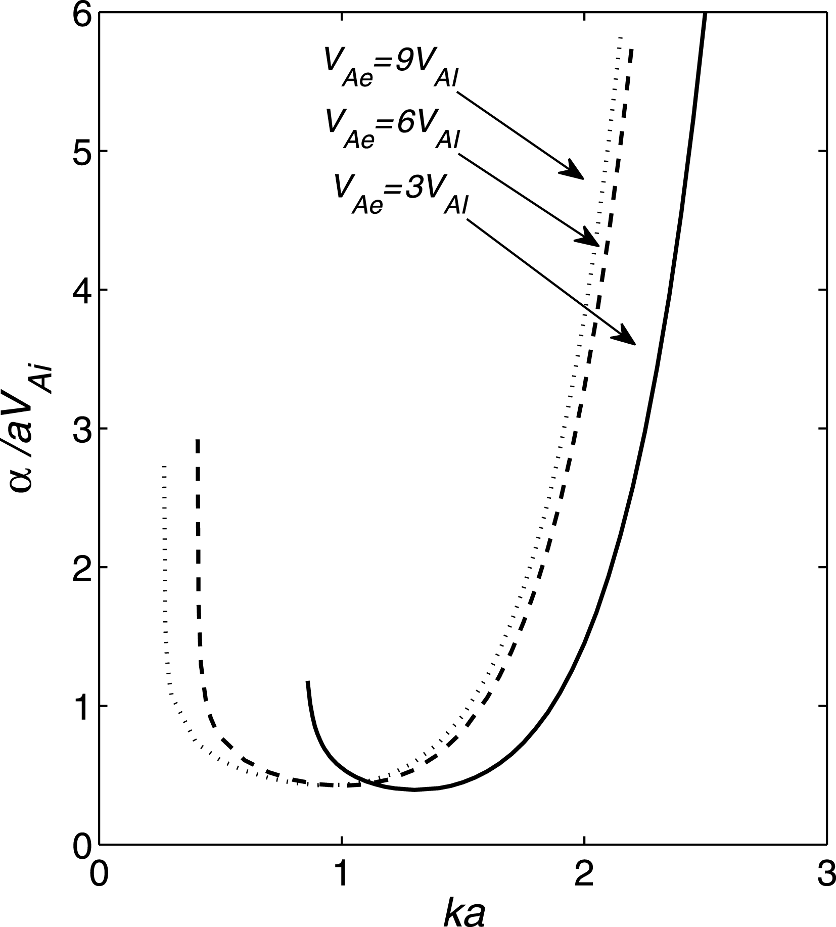
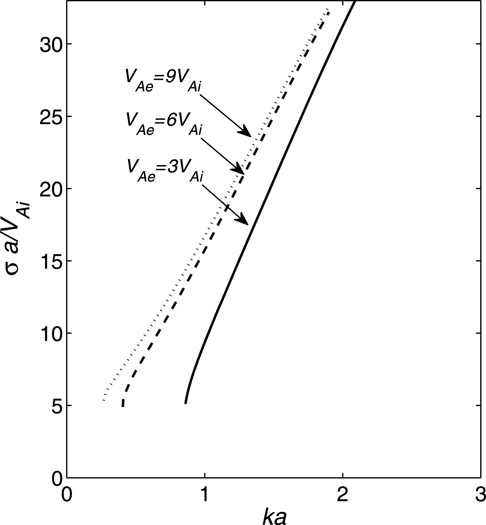
The quantities ${\it\alpha}$ and ${\it\sigma}$ have been calculated numerically for various values of the parameters (see figures 2 and 3). Returning to the original non-scaled variables, we rewrite (5.53) as

(5.57) $$\begin{eqnarray}\text{i}\left(\frac{\partial u}{\partial t}+V_{g}\frac{\partial u}{\partial z}\right)+{\it\alpha}\frac{\partial ^{2}u}{\partial z^{2}}+{\it\sigma}u|u|^{2}=0,\end{eqnarray}$$

where $u={\it\epsilon}A$ . We see in figure 2 that ${\it\alpha}>0$ . This result agrees well with the shape of the dispersion curves for fast sausage waves. It can be seen in the dispersion diagram for these waves that the dispersion curves are convex (see, e.g. Edwin & Roberts Reference Edwin and Roberts1983). The expression for ${\it\sigma}$ is very complex, so it is extremely difficult to prove rigorously that ${\it\sigma}>0$ . However, we found numerically that this is true for a very wide range of parameter values (see figure 3). Hence, it appears to be reasonable to make the conjecture that ${\it\sigma}>0$ for all parameter values. This implies that (5.57) is the focusing NLS equation.

Figure 2.

The dependence of coefficient ${\it\alpha}$ on the dimensionless wavenumber $ka$ . The solid, dashed and dotted lines correspond to $V_{Ae}/V_{Ai}=3,6$ and $9$ .

Figure 3.

The dependence of coefficient ${\it\sigma}$ on the dimensionless wavenumber $ka$ . The solid, dashed and dotted lines correspond to $V_{Ae}/V_{Ai}=3,6$ and $9$ .

It is worth recalling that (5.57) was derived under the assumption that the magnetic tube has the sharp boundary. Nakariakov & Roberts (Reference Nakariakov and Roberts1995) studied fast linear kink waves in a magnetic slab with a smooth Alfvén velocity profile. They found that the behaviour of the group speed in the case of a very smooth velocity profile is quite different from that for the case where this profile is steep. In the first case, the group velocity is a monotonically decreasing function of the wavenumber, meaning that $\text{d}^{2}{\it\omega}/\text{d}k^{2}<0$ . In the second case, the group velocity has a minimum, meaning that $\text{d}^{2}{\it\omega}/\text{d}k^{2}<0$ for small $k$ , while $\text{d}^{2}{\it\omega}/\text{d}k^{2}>0$ for large $k$ . By analogy, we can assume that the result $\text{d}^{2}{\it\omega}/\text{d}k^{2}>0$ , obtained in this paper under the assumption that the tube has the sharp boundary, may not be valid in the case of a tube with a continuous density variation in the radial direction. We emphasise that Nakariakov & Roberts (Reference Nakariakov and Roberts1995) obtained their result for the Epstein profile and in a planar geometry. Hence, it would be wrong to assume a complete analogy between the cylindrical geometry with an arbitrary smooth density variation and the case studied by Nakariakov & Roberts (Reference Nakariakov and Roberts1995). We mention their study only as a cautionary example.

6. Implication for solar physics

Equation (5.57) has a few families of exact solutions (see, e.g. Zhelyazkov et al. Reference Zhelyazkov, Murawski, Goossens, Nenovski and Roberts1994) in the form of stationary waves. This family includes, in particular, bright envelope soliton with the amplitude tending to zero at infinity. Another interesting property of this equation is related to the stability of the solution in the form of a harmonic wave given by

(6.1) $$\begin{eqnarray}u=u_{0}\exp (\text{i}kz-\text{i}{\it\omega}t),\quad {\it\omega}=V_{g}k+{\it\alpha}k^{2}-{\it\sigma}u_{0}^{2},\end{eqnarray}$$

where $u_{0}$ is a constant amplitude. Since ${\it\alpha}{\it\sigma}>0$ , the solution is subject to the modulational or Benjamin–Fair instability (e.g. Zakharov & Ostrovsky Reference Zakharov and Ostrovsky2009). The development of this instability may, in particular, result in the appearance of envelope solitons. Finally, (5.57) admits various solutions describing the rogue waves (see, e.g. Dubard et al. Reference Dubard, Gaillard, Kleina and Matveev2010).

As we have already stated in § 1, in application to solar physics, the fast sausage waves are used to explain the observed QPPs of electromagnetic emission generated by solar flares. Sometimes QPPs with two, or even a few, different periods are observed simultaneously. One such observation was reported by Su et al. (Reference Su, Shen, Liu, Liu and Mao2012). Both pulsations with periods $P<60$  s and $P>60$  s have been observed. The propagation speed of pulsations with shorter periods was larger than that of pulsations with longer periods. The authors suggested that the pulsations with shorted periods were due to fast sausage waves, while those with longer periods were caused by slow magnetosonic waves. We can suggest an alternative explanation of these observations. While we do not question the suggestion that the pulsations with shorter periods were caused by fast sausage waves, we can suggest that the pulsations with longer periods appear due to the modulational instability. The periods of envelope waves are substantially larger than that of the carrier wave. The phase speed of envelope waves is $V_{g}$ , which is usually substantially smaller than the phase speed ${\it\omega}/k$ of the carrier wave (e.g. Oliver et al. Reference Oliver, Ruderman and Terradas2015, see their figure 2).

The solutions of the focusing NLS equation in the form of freak waves can explain why the QQPs are usually have short duration, usually only a few oscillation periods are observed. This is simply a typical property of freak waves.

7. Summary and conclusions

In this paper we derived the nonlinear Schrödinger equation for fast sausage waves in magnetic tubes. We assumed that the tube is straight and homogeneous, meaning that the densities inside and outside the tube are constant. To describe the wave motion we used the cold plasma approximation. We then used multiscale expansions. The coefficients of the nonlinear Schrödinger equation were expressed in terms of Bessel and modified Bessel functions. They were evaluated numerically for various values of the parameters. In particular, it was shown that the criterion for the onset of the modulational, or Benjamin–Fair, instability is satisfied.

We discussed the implication of the obtained results for solar physics. In particular, we speculated that the development of the modulational instability can explain simultaneous observations of QPPs with short and long periods. We suggested that the short period QPPs can be caused by the fast sausage carrier wave, while the long period QPPs are related to envelope waves which appear due to the modulation instability. We also suggested that the solutions describing freak waves can be used to explain why QPPs are only observed during a few oscillation periods.