




1. Introduction
Globular clusters (GCs) are expected to have hundreds to thousands of black holes (BHs) born during their formation, but our understanding of the present day populations and distribution of these BHs is limited. By uncovering the distribution of BHs in GCs, we can gain a better understanding of potential Laser Interferometer Gravitational-Wave Observatory (LIGO) sources and where they originate, as well as understand the impacts that natal kicks have on the retention of BHs in star clusters. By searching for microlensing signatures within Omega Centauri (
 $\omega$
Cen), we can discover potential BH candidates and begin to answer these open questions.
 $\omega$
Cen is a prime candidate to learn more about the questions proposed above. It is the most massive GC in the Milky Way, with a mass of 3.55e6
 $\text{M}_\odot$
(Baumgardt & Hilker Reference Baumgardt and Hilker2018). This large mass translates into a high number of BHs initially formed and a high retention fraction due to the increased escape velocity. Not only is
 $\omega$
Cen the most massive GC, but it has also been observed extensively by the Hubble Space Telescope (HST) in the past 20 years. This temporal coverage is well matched to the duration of microlensing events that we expect to observe (roughly 1 year timescales, see Reference Zaris, Veske and SamsingZaris et al. (2020)).
Dynamical studies have shown the need for a dark mass at the center of
 $\omega$
Cen, but it has long been discussed whether this dark mass is an intermediate-mass black hole (IMBH) (Noyola et al. Reference Noyola, Gebhardt and Bergmann2008; Noyola et al. Reference Noyola, Gebhardt and Kissler-Patig2010; Baumgardt Reference Baumgardt2017) or can be explained by other properties (Anderson & van der Marel Reference Anderson and van der Marel2010; van der Marel & Anderson Reference van der Marel and Anderson2010; Zocchi et al. Reference Zocchi, Gieles and Hénault-Brunet2017). Zocchi et al. (Reference Zocchi, Gieles and Hénault-Brunet2019) and Baumgardt et al. (Reference Baumgardt, He and Sweet2019) showed that a centrally concentrated cluster of stellar mass black holes is able to explain the observed kinematics. Häberle et al. (Reference Häberle, Neumayer and Seth2024) recently added to this debate with the discovery of multiple fast-moving stars in the innermost region of
 $\omega$
Cen, providing strong evidence for an IMBH, but this finding does not exclude a significant mass contribution from stellar mass black holes.
The expected lensing events are expected to be firmly in the microlensing regime, where we see an increase in apparent brightness, but with the lensing scale far below our telescope resolution. We use the
 $\sim$
500 HST exposures to search for microlensing signatures in the lightcurves of source stars caused by potential black hole lenses.
In Section 2, we describe the regression model we use to fit microlensing events, as well as the synthetic data set we use to tune our model and determine our completeness. Then, in Section 3, we detail the methods that we use to find lightcurves with potential microlensing events. Finally, in Section 4, we conclude this work and describe ongoing efforts.
2. Synthetic Microlensing Lightcurves
We use the set of microlensing equations, as derived by Einstein (Reference Einstein1936) and taken here from Schneider (Reference Schneider2006), to create a regression model to help identify potential lensing events in the data and to create synthetic microlensing events.
Using star cluster simulations (see Prieto et al. Reference Prieto, Rodriguez and Cabrera2025), we can determine the distribution of microlensing parameters to create realistic synthetic events. We can then sample the distributions and inject the synthetic microlensing events into the lightcurves of the real data. To prevent any potential real microlensing events leaking into the synthetic data, we bootstrap over the epochs of the observations; this preserves our observational cadence and
 $\sigma_G$
values (a robust standard deviation estimate that is less impacted by outliers, defined as:
 $\sigma_G = 0.7413 * (q75 - q25)$
, where q75 and q25 are the 75th and 25th quartiles, respectively). We created 40,000 synthetic lightcurves with injected synthetic microlensing events.
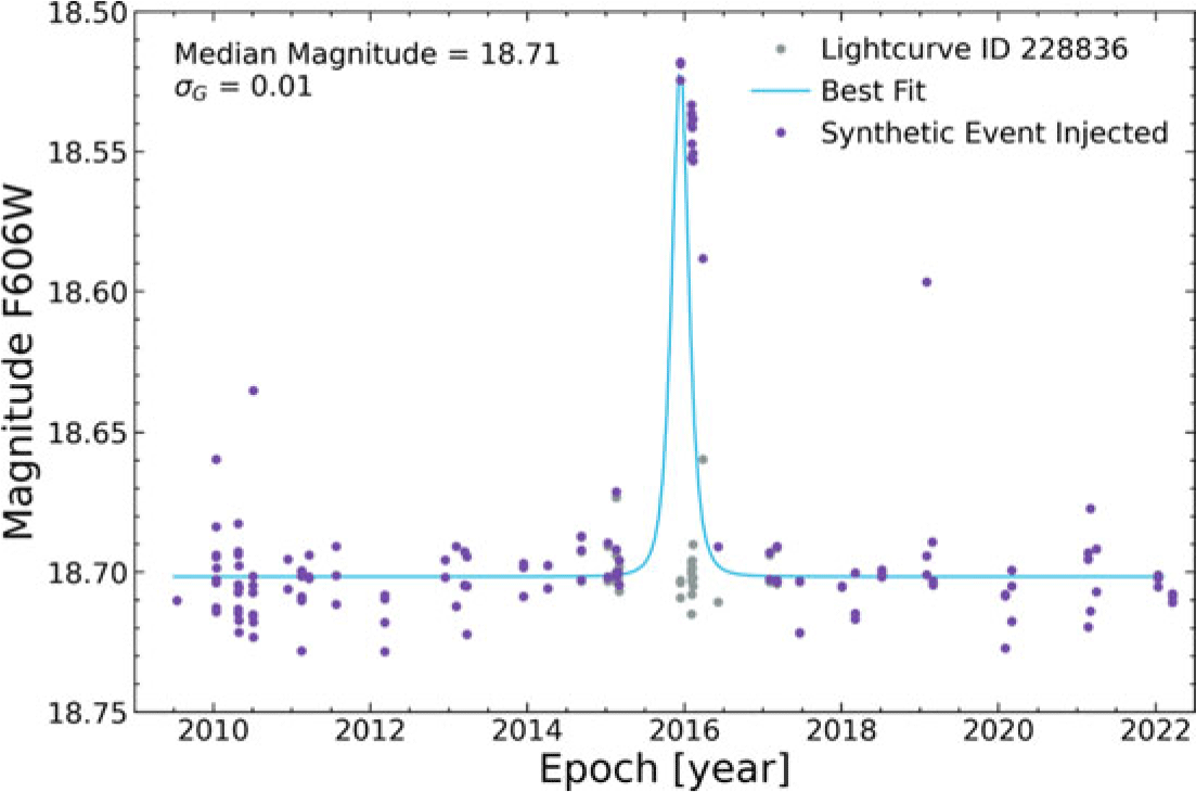
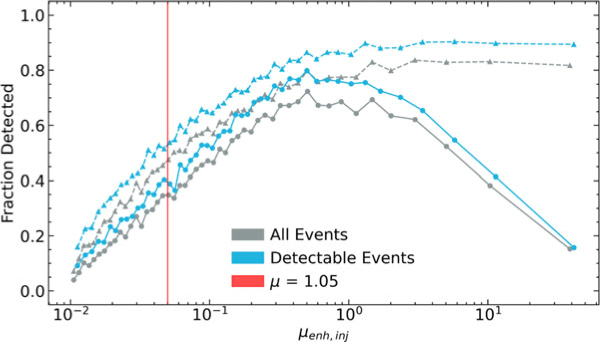
We are then able to use our regression model (using the Bayesian framework, Maximum a Posteriori, where we use the magnification distribution from simulations as a prior distribution) to fit our lightcurves. An example of a synthetic lightcurve with a synthetic microlensing event injected can be seen in Figure 1, with the regression model best fit plotted as the light blue line. We then are able to fit the set of 40,000 synthetic lightcurves, allowing us to estimate our completeness, which can be seen in Figure 2.
Lightcurve ID 228836 shown as the gray points. This lightcurve has a median magnitude = 18.71 and a
 $\sigma_G$
= 0.01. The purple points show lightcurve ID 228836 with an injected synthetic lensing event. Injected values: max magnification = 1.2, epoch of max magnification = 2016, tranverse velocity = 16.8 km/s, distance between lens and source = 4 parsecs (pc). The blue line shows the best fit to the synthetic lightcurve.

This figure shows the fraction of recovered events as a function of the enhanced injected magnification. The dashed lines with triangle markers represent events where the date was recovered, while the solid lines with circle markers represent where the date was recovered and was within 80% of the enhanced injected magnification. Each point contains 800 synthetic lightcurves; the enhanced injected magnification is the median value of the bin members.

3. Searching for Microlensing Events
Although we can fit our synthetic lightcurves with the regression model described in Section 2, it is difficult to determine which fits are truly potential microlensing events. For example, a spurious bright outlier could cause a large magnification fit; based on the fit parameters, it may seem at first to be a potential lensing event that we would want to inspect, but upon further inspection, it would be realized as a false positive. Since we know the synthetic lightcurves have synthetic events, we expect any real event to have statistics similar to those of our synthetic events; therefore, we can use post-regression statistics calculated on our real and synthetic lightcurves to assist in the search.
We calculated 2D histograms from two statistics of our real and synthetic lightcurves, counting the number of each in every bin (
 $n_{synth}$
and
 $n_{real}$
), then for each bin we calculated the ratio
 $n_{synth} / (n_{synth} + n_{real})$
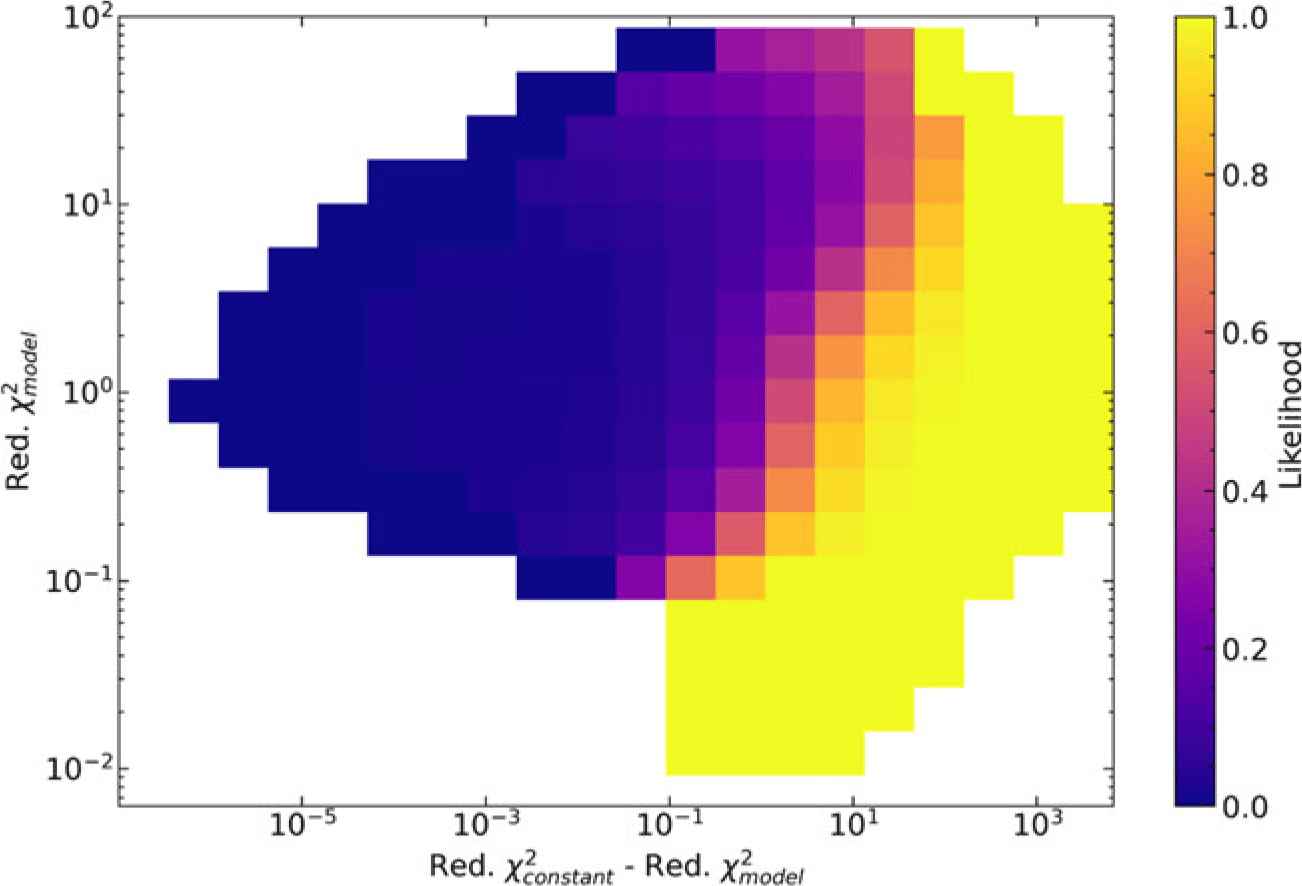
. This serves as an ad hoc likelihood of a lensing event being found in a lightcurve, where bin values closer to 1 suggest that a real lightcurve closely resembles synthetic lightcurves. We show an example of this approach in Figure 3, where the first statistic is the reduced chi-square value of the model fit,
 $Red. \chi^2_{model}$
, and the second statistic is the difference between the reduced chi-square value of a constant line,
 $Red. \chi^2_{constant}$
and
 $Red. \chi^2_{model}$
. When this difference is large, the model has a statistically better fit than the constant line. For a given lightcurve, we can then determine what bin it falls within and the corresponding likelihood, and prioritize our search in this way.
The difference in reduced chi squares between a constant line fit and the model line fit vs. the reduced chi square of the model line fit. Larger values along the x-axis indicate that the model line fit is statistically better than the constant line fit. The color bar represents an ad hoc likelihood, calculated by counting the number of lightcurves (synthetic and real) in each bin and using the equation
 $n_{synth} / (n_{synth} + n_{real})$
. Real lightcurves in bins with lighter colors in the plot indicate a higher likelihood of a potential lensing event. A Gaussian kernel with a standard deviation of 1 has been applied to smooth the features.

Figure 3 Long description
A heat map representing the difference in reduced chi squares between a constant line fit and a model line fit on the x-axis and the reduced chi square of the model line fit on the y-axis. The color bar indicates an ad hoc likelihood, with lighter colors representing a higher likelihood of a potential lensing event. The heat map uses a grid layout with a logarithmic scale on both axes. Higher values along the x-axis indicate that the model line fit is statistically better than the constant line fit. A Gaussian kernel with a standard deviation of 1 has been applied to smooth the features.
4. Conclusion and Future Work
Candidate follow-up is currently ongoing with the approach detailed in Section 3, in addition to neural network approaches, where the post-regression statistics can be fed into a neural network which then outputs a likelihood of lensing. This allows for the use of many different post-regression statistics to be used as input features and to model more complicated spaces, rather than the relatively small number of statistics that can be used with the 2D histogram approach.
Acknowledgments
Also contributing: Anil C. Seth, Maximilian Häberle, Andrea Bellini, Callie Clontz, Sebastian Kamann, Mattia Libralato, Nadine Neumayer, Carl Rodriguez, Jay Strader, Doga Veske, John Zaris. This project was funded in part by Hubble Space Telescope archival grant AR 17033.
 σG
 nsynth/(nsynth+nreal)

 Open access

