


1. Introduction
It is well known that global climatic warming may cause sea-level rise via melting of glaciers and ice sheets, shrinking of the sea-ice cover and expansion of the volume of the oceans. Relationships and observations are summarized in the assessment reports of the Intergovernmental Panel on Climate Change (IPCC) (Reference Warrick, Oerlemans, Houghton, Jenkins and EphraumsWarrick and Oerlemans, 1990; Reference Pachauri and ReisingerPachauri and Reisinger, 2007; Reference SolomonSolomon and others, 2007). While most publications agree that sea level is currently rising, the estimated amount of future sea-level change varies widely across published studies, despite sea-level rise being a potential threat for societies, and not only those in regions with low elevations above common sea level. This motivates modeling of future sea-level rise and estimating the maximal sea-level rise over the medium-range future. The multitude of physical processes contributing to sea-level change necessitates in-depth studies that will be summarized in the next IPCC report (Fifth Assessment Report (AR5)), and new observations, as well as recent improvements in physical models, facilitate a more accurate assessment. This study is motivated by the need to accurately predict that part of sea-level rise that is caused by mass loss from the Greenland ice sheet, a goal that is shared with SeaRISE (Sea-level Response to Ice Sheet Evolution), a US-led community organized effort to estimate the upper bound of ice-sheet contributions to sea level in the next centuries (http://websrv.cs.umt.edu/isis/index.php/SeaRISEAssessment) and ice2sea, a science program funded by the European Union Framework-7 scheme to improve projections of the contribution of ice to future sea-level rise (http://www.ice2sea.eu/). Both efforts rely on dynamic ice-sheet models to predict future changes in ice dynamics and in sea level.
Our study addresses a specific problem in connecting observations and models that has not received much attention to date. It is well known that mass transfer from ice sheet to ocean occurs largely through outlet glaciers via calving and meltwater processes. In many cases, the outlet glaciers have a higher velocity than the neighboring inland ice, and often the acceleration is caused by the existence of a morphological trough or trough system in the bedrock. In addition, the fast-moving outlet glaciers of the Greenland and Antarctic ice sheets tend to react most rapidly to warming (e.g. Reference WeidickWeidick, 1984; Reference KrabillKrabill and others, 1999; Reference Mayer and HerzfeldMayer and Herzfeld, 2001, Reference Mayer and Herzfeld2008; Reference Johnson, Prescott and HughesJohnson and others, 2004; Reference ThomasThomas and others, 2004; Reference Hall, Williams, Luthcke and DigirolamoHall and others, 2008; Reference Van de WalVan de Wal and others, 2008; Reference Box, Yang, Bromwich and BaiBox and others, 2009). Subglacial trough systems have largely been unrepresented in the subglacial topography dataset utilized by modeling groups. For instance, SeaRISE initially used the bed topography derived by Reference Bamber, Layberry and GogineniBamber and others (2001), which does not include the trough of Jakobshavn Isbræ (Ilulissat Ice Stream), the fastest-moving and most studied ice stream in Greenland, which drains 6% of the Greenland ice sheet and retreated during 1999–2007 (Reference Echelmeyer and HarrisonEchelmeyer and Harrison, 1990; Reference Echelmeyer, Clarke and HarrisonEchelmeyer and others, 1991, Reference Echelmeyer, Harrison, Clarke and Benson1992; Reference Podlech and WeidickPodlech and Weidick, 2004; Reference Mayer and HerzfeldMayer and Herzfeld, 2008).
Collection of a more accurate representation of the bed topography (the objective of NASA’s Operation IceBridge, undertaken by the Center for Remote Sensing of Ice Sheets (CReSIS) over the last several years) does not, however, directly provide a solution to the modeling community, as most subglacial troughs have a spatial scale close to or smaller than the scale used in dynamic ice-sheet models. Data collection is underway to further refine the bed representation, especially along the ice-sheet margins, but comparative experiments conducted community-wide for AR5, such as those of SeaRISE, are typically run at 5 km grid scale.
Flight-line data for ice thicknesses have very high resolution along the flight-line but lower resolution between the flight-lines (~1 to 5 km), from which uniformly gridded digital elevation models (DEMs) are created. Problems associated with the approach to interpolation are beyond the scope of this paper; suffice it to say that the DEMs produced are often at higher resolution than is practical with current whole-ice-sheet models and must be degraded. The SeaRISE experiments are being carried out at 5 km, a resolution that makes runtimes reasonable enough to allow a suite of experiments to be performed. Simply averaging the bed data in a mathematical or geostatistical sense broadens and flattens the troughs. Nearest-neighbor selection can lead to discontinuities in the geologic feature. A new algorithm, termed the JakBed algorithm, has been designed, that employs principles from algebraic topology and mathematical morphology to retain morphologic properties and correct depths of troughs in bed topography at the lower resolution needed by the modeling community (e.g. a 5 km grid; Reference Herzfeld, Wallin, Leuschen and PlummerHerzfeld and others, 2011). This bed was adopted by SeaRISE in 2010 and motivated further research on mathematical modeling of bed topography and its relevance for dynamic ice-sheet models. The JakBed algorithm has been generalized and applied to four major outlet glaciers and glacier systems, Jakobshavn Isbræ, Helheim Glacier, Kangerdlussuaq Glacier and Petermann Gletscher regions, selected because of their glaciological importance and because airborne radar measurements of sufficient density and coverage are available (Reference Herzfeld, McDonald, Wallin, Chen, Leuschen and PadenHerzfeld and others, submitted).
The objective of this paper is to investigate the effect of including the more accurately represented subglacial topography, by comparing the responses of two ice-dynamic models run with two 5 km bed DEMs that differ only in the regions including the four ice streams. Sensitivity of model output, such as surface velocity field and basal water production, is examined at a fixed time, and differences in predicted response to an enhanced basal sliding experiment are performed. Change in volume loss resultant from use of the new bed DEM is calculated.
2. Approach
The problem of studying the effect of subglacial topography on results from dynamic ice-sheet models spans a suite of investigations: (1) radar data analysis and interpolation; (2) development and application of algorithms for inclusion of sub-scale topographic relief of troughs in a DEM of bed topography at a lower, 5 km, scale; (3) comparative runs with several dynamic ice-sheet models; (4) analysis of the sensitivity of modeled variables dependent on bed topography (investigation of the effects on ice surface velocity and the potential for basal sliding to occur as indicated by presence of water in the bed); and (5) assessment of relevance of improved subglacial topography for modeled ice-volume evolution. Ice-volume loss derived in (5) is given as the increase in sea-level equivalent. Topics (1) and (2) are treated by Reference Herzfeld, McDonald, Wallin, Chen, Leuschen and PadenHerzfeld and others (submitted) and summarized in Section 2.1.
2.1. Linking data and models
Subglacial troughs are important in controlling the dynamics of ice streams, including observed acceleration of ice flow over deep troughs, shear across the margins, separation of fast-flowing ice streams and slow-moving inland ice, and extension of the fast movement into the drainage basin upstream of the main trough. These effects are manifested in topographically induced crevasse patterns at the ice surface, which are visible in satellite imagery (Figs 1–4). Typically, the region of fast movement extends several kilometers upstream of the crevassed area, because the occurrence of crevassing requires that the ice accelerates beyond a threshold, at which brittle deformation rather than ductile deformation takes place. The relationship between subglacial trough location, ice acceleration, crevassing over the ice stream and shear margins is best demonstrated for Jakobshavn Isbræ South Ice Stream, whereas the North Ice Stream is not topographically induced Fig. 1) (Reference Mayer and HerzfeldMayer and Herzfeld, 2001).Helheim Glacier has five branches that are separated by nunataks (Fig. 2). For Kangerdlussuaq Glacier, crevasse patterns indicate that surface velocity is high in a triangular area upstream of the calving front that includes three fast-moving branches (Fig. 3).
Jakobshavn Isbræ (Ilulissat Ice Stream) surface structure, crevassing and subglacial topography. Terra ASTER (Advanced Spaceborne Thermal Emission and Reflection Radiometer) data (band 1,2,3 color composite) collected May 2003 show calving front and crevassing indicative of fast-moving ice and the shear margin. Subglacial topography contoured from CReSIS MCoRDS data. Jakobshavn Isbræ South Ice Stream follows a deep subglacial trough. Universal Transverse Mercator coordinates.

Helheim Glacier surface structure and crevassing. Helheim Glacier is the large glacier that enters Sermilik fjord from the west and has five branches separated by nunataks. The regions of fast flow coincide with crevasse fields, which appear as darker areas in the satellite image. The surface flow field is visible in the flowbands in the image. Image downloaded from GoogleMaps (http://maps.google.com) 5 March 2012. Image area LL (–38.833923° E, 66.190466° N), UR (–37.400208° E, 66.637734° N), LR (–37.400208° E, 66.190466° N), UL (–38.831177° E, 66.636645° N).

Kangerdlussuaq Glacier surface structure and crevassing. Kangerdlussuaq Glacier is the large glacier that enters the fjord from the northwest. Crevasse patterns indicate that surface velocity is high in a triangular area upstream of the calving front. The surface flow field is visible in the flowbands in the image. Image downloaded from GoogleMaps (http://maps.google.com) 5 March 2012. Image area LL (–34.170227° E, 68.367814° N), UR (–32.308502° E, 68.910017° N), LR (–32.305756° E, 68.367814° N), UL (–34.164734° E, 68.909028° N).

Petermann Gletscher surface structure, crevassing and calving. Petermann Gletscher is the large glacier that enters the fjord from the south. (a) Surface structure and crevassing in the Petermann Gletscher region in July 2003. Moderate Resolution Imaging Spectroradiometer (MODIS) data, NASA Terra satellite, 5 July 2003. Figure is a subimage of data downloaded from http://eoimages.gsfc.nasa.gov/images/imagerecords/7000/7999/greenland tmo 2003186 lrg.jpg on 5 March 2012. Petermann Gletscher has a large floating tongue (the largest in the Northern Hemisphere) that calves icebergs. (b) MODIS image of Petermann Gletscher taken 10 hours after a calving event on 5 August 2010 18:05 UTC (data acquisition time); this is the largest iceberg calved since 1962. Information and data downloaded from http://earthobservatory.nasa.gov/NaturalHazards/view.php?id=45112 on 5 March 2012. Note that floating tongues and calving processes are not included in the models. Image area LL (–51.086426° E, 79.570495° N), UR (–55.92041° E, 82.267614° N), LR (–62.644043° E, 79.071812° N), UL (–68.730469° E, 81.779929° N).

The observation of links between subglacial topography and ice dynamics motivates the derivation of a trough-bed algorithm, which, in a nutshell, allows the retention of features that are smaller than or on the order of the resolution of the resulting computational grid, in particular the troughs. The modeled glacier bed is required to have the following properties: (1) to preserve the correct locally maximal depth of the trough; (2) to represent the trough as continuous; and (3) to morphologically model the rim of the trough as rounded by erosion. The algorithm for inclusion of troughs consists of the following steps:
-
1. Identification of trough locations by tracing the canyon bottom as a topologically simply connected line, which is edge-connected in the discretization of gridcells.
-
2. Adjustment of high-resolution grid to trough locations to preserve morphologic characteristics.
-
3. Assignment of locally maximal trough depths for gridcells that are trough locations.
Reference Herzfeld, Wallin, Leuschen and PlummerHerzfeld and others (2011) give a full description of the algorithm used to generate the Jakobshavn bed. Reference Herzfeld, McDonald, Wallin, Chen, Leuschen and PadenHerzfeld and others (submitted) describe a generalization of this algorithm to trough systems with several branches and different directions (as needed for Helheim, Kangerdlussuaq and Petermann glaciers).
Data
Data used for the improved Greenland bed DEM were collected with the Multichannel Coherent Radar Depth Sounder (MCoRDS) by CReSIS (Gigineni and others, 2001; Reference LohoefenerLohoefener, 2006; see http://www.cresis.ku.edu/research/techreports/TechRpt109.pdf).
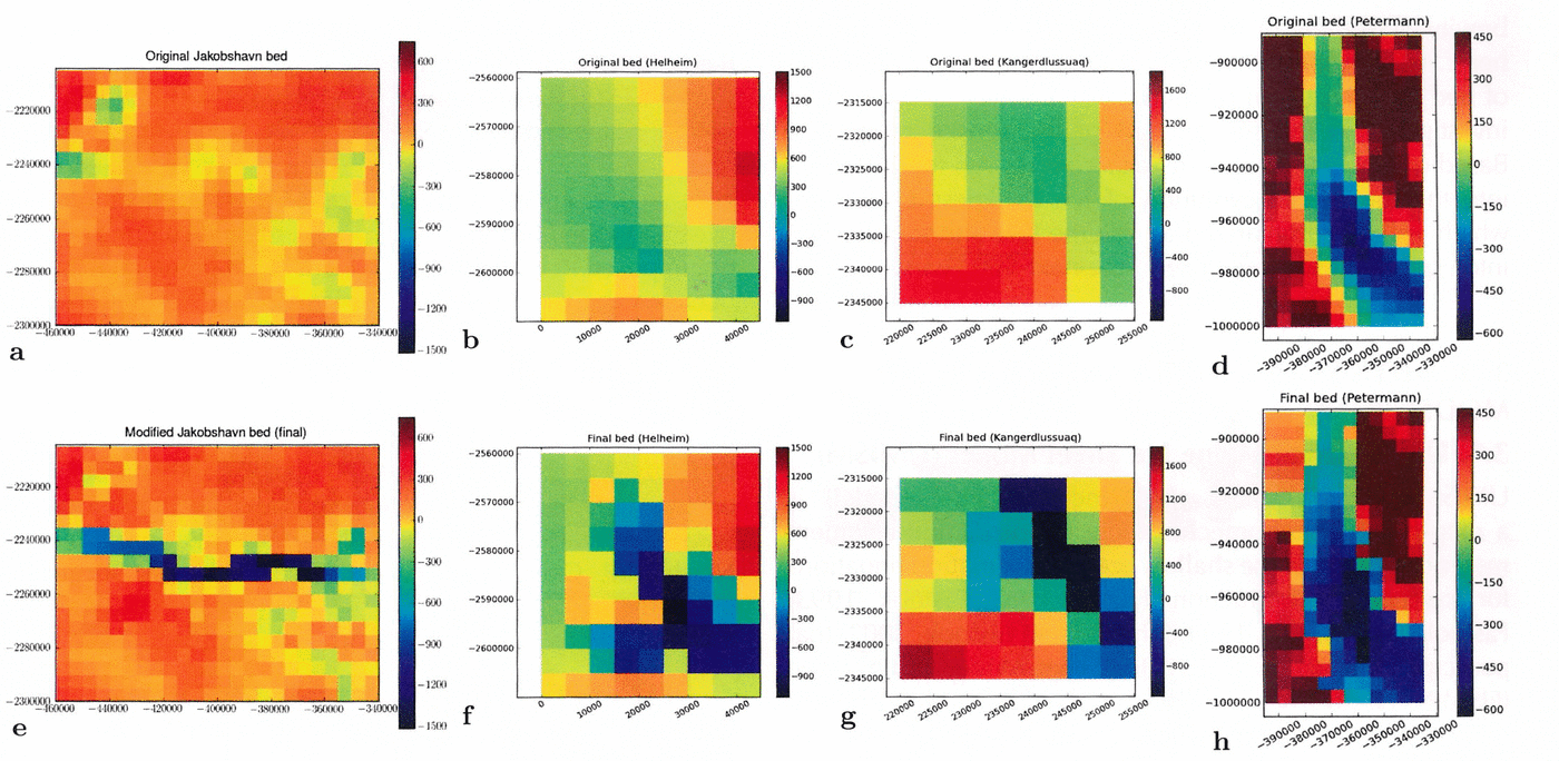
Based on regional coverage of MCoRDS data, the trough-bed algorithm was applied to generate new regional DEMs for the following regions (Fig. 5):
Trough systems in 5 km subglacial topography: Jakobshavn Isbræ, Helheim Glacier, Kangerdlussuaq Glacier and Petermann Gletscher. (a–d) Original bed V0.93 (Reference Bamber, Layberry and GogineniBamber and others, 2001), (e–h) JakHelKanPet bed. (a, e) Jakobshavn Isbræ region; (b, f) Helheim Glacier region; (c, g) Kangerdlussuaq Glacier region; (d, h) Petermann Gletscher. (a–h) Subglacial elevation in meters above WGS84. Polar stereographic coordinates with central meridian –39.0°E , 90.0° N, latitude of true scale 71.0° N, WGS84 (SeaRISE-type).
Jakobshavn Isbræ (–50.297884° E, 68.634417° N) (lower left map corner) to (–47.641955° E, 69.727571°N) (upper right map corner),
Helheim Glacier (–39.109514° E, 66.308344° N) (lower left map corner) to (–37.997541° E, 66.757817° N) (upper right map corner),
Kangerdlussuaq Glacier (–33.696239° E, 68.543468° N) (lower left map corner) to (–32.697422° E, 68.841516°N) (upper right map corner) and
Petermann Gletscher (–60.481399° E, 80.081021° N) (lower left map corner) to (–59.337720° E, 81.293184° N) (upper right map corner).
The resultant trough systems in the new JakHelKanPet (or JHKP) bed DEM (Greenland 5km JHKP.nc) are shown in Figure 5, along with the same areas in the bed DEM of Reference Bamber, Layberry and GogineniBamber and others (2001) that was originally proposed for use in the SeaRISE experiments. For Jakobshavn South, Helheim and Kangerdlussuaq glaciers, the crevassed regions coincide with the trough locations (compare Figs 1–4 with Fig. 5). Note that for Petermann Gletscher the situation is different, as it has the largest floating tongue in the Northern Hemisphere, calves large icebergs and has a surface structure characterized by longitudinal runnels; the grounding line is near the head of the fjord (Fig. 4) (Reference Rignot and SteffenRignot and Steffen, 2008; Reference Johnson, Münchow, Falkner and MellingJohnson and others, 2011). Considering that grounding lines are not included in models, different responses may be expected.
Integration into modeling datasets and availability
The trough and trough-system regions are integrated seamlessly into an existing Greenland bed DEM (identity map around the subregion edges with a decay of the morphological model towards the edges). The algorithm allows integration into any 5 km DEM of Greenland of the same type and projection. In this study we use Greenland 5km v0.93.nc, available at the SeaRISE data wiki (http://websrv.cs.umt.edu/isis/index.php/SeaRISE Assessment). The new dataset (Greenland 5km JHKP.nc) is available from the ftp site of the first author and from the SeaRISE data wiki.
Structure of modeling datasets
To provide a user-friendly dataset to the modeling community, we have used the portable and compact netcdf format, as defined by SeaRISE, that includes latitude and longitude, as well as the same stereographic projection onto a 5 km-resolution (x-y) grid of the following data useful to an ice-sheet model: surface elevation; ice thickness; bed elevation; rate of change of the ice surface; measured surface velocity (magnitude, x and y components); balance velocity magnitude; present precipitation; present air temperature; geothermal heat flux; and a land-cover mask. Also included are ice-core isotopes and sea level as a function of time for at least one glacial/interglacial cycle (http://websrv.cs.umt.edu/isis/index.php/SeaRISE Assessment). For UMISM (the University of Maine Ice Sheet Model) runs, the precipitation and temperature used are those provided by Reference EttemaEttema and others (2009). SICOPOLIS (SImulation COde forPOLythermal Ice Sheets) runs use the precipitation of Reference EttemaEttema and others (2009) and the temperature parameterization of Reference Fausto, Ahlstrøm, Van As, Bøggild and JohnsenFausto and others (2009). In the model experiments described below, only the bed topography input is varied (SeaRISE dataset Greenland 5km v0.93.nc in one run, dataset Greenland 5km JHKP.nc in the other); all other input is kept the same.
2.2. Modeling experiments
The goal here is to optimally bridge between observation and modeling efforts. Observations are not spatially uniform and may be closely spaced in one area and scant in another, while the resolution realizable in a model is limited by computational resources, including runtime and memory. While data collection may improve in the future, both in areal coverage and resolution, and while model resolutions will certainly increase, the role of our algorithm is to be able to obtain better results from presently collected data with current modeling techniques.
To test this working hypothesis and to quantify the importance of bedrock topography in dynamic modeling and prediction of ice-volume change, we perform several case studies with the two ice-sheet models UMISM (Reference FastookFastook, 1993; Reference Fastook and PrenticeFastook and Prentice, 1994) and SICOPOLIS (Reference GreveGreve, 1995, Reference Greve1997; Reference Greve and BlatterGreve and Blatter, 2009), keeping all input variables constant and varying the bed topography (SeaRISE dataset Greenland 5km v0.93.nc vs dataset Greenland 5km JHKP.nc).
Assessment of the influence of outlet glaciers in bed topography on results from dynamic ice-sheet models will be conducted in two series of experiments: (1) in reconstructions of present-day conditions, especially of surface velocities and basal sliding potential, resulting from so-called model spinups, and (2) in predictions of ice-volume changes for the next 500 years.
The primary diagnostics of differences in the response of the various ice-sheet models to the improved bed DEM are the surface ice velocities and the production of water at the bed for a time snapshot intended to correspond to the present time for the ice sheet. This time snapshot is generated differently for each of the models, but basically requires some ‘spin-up’ of the models by running for a sufficient time period with specified climate variation, so that the configuration matches as closely as possible the observed non-steady-state ice sheet.
Changes in the Greenland ice sheet and its outlet glaciers relevant for assessment of sea-level rise have two main components: (1) mass loss from melting due to climate change, and (2) acceleration of outlet glaciers, which may occur as part of a surge cycle or tidewater cycle or be caused by changes in the mechanical properties of the ice or changes in the basal conditions that allowor enhance sliding. Analysis of the modeled surface velocity resulting from the use of different bed representations allows us to assess the importance of a correct representation of the model-input bed.
Because basal sliding is a key component in determining the velocity of outlet glaciers, and because basal sliding potential is directly related to the amount and character of water present at or near the bed of the glacier, the amount of water produced at the bed is another key diagnostic in assessing the importance of an accurately represented bed. Because thicker ice is more likely to reach the pressure-melting point at the bed and begin to produce meltwater at the bed, the depth of the glacier bed in a trough is directly related to basal sliding. The different mechanisms whereby each model implements the onset of sliding and its connection to basal melting are explained in Sections 3.1 and 3.2.
Other variables (e.g. surface mass balance, surface elevation and resultant mass loss) are affected by changes in surface velocity and basal sliding potential in a model. For brevity, sensitivity of these other variables is not analyzed here. As the ultimate consequence of modeling, the effect of bed topography on predicted ice-volume change will be investigated in the second part of the sensitivity studies. Based on comparative model experiments run for 500 years into the future, the evolution of ice thickness is derived, which will be summarized as volume loss and transformed into equivalent sea-level rise in the next 500 years.
3. Ice-Dynamic Models and Set-Up of Model Runs
3.1. University of Maine Ice Sheet Model (UMISM)
UMISM (the University of Maine Ice Sheet Model) is a map-plane, thermomechanically coupled, finite-element method solution of the shallow-ice approximation equations for ice-sheet reconstruction (Reference HutterHutter, 1983; Reference FastookFastook, 1993; Reference Fastook and PrenticeFastook and Prentice, 1994; Reference Johnson and FastookJohnson and Fastook, 2002) that participated in the European Ice-Sheet Modelling Initiative (EISMINT) model-intercomparison exercise (Reference Huybrechts and PayneHuybrechts and others, 1996; Reference PaynePayne and others, 2000). Basic input includes bed elevation, mean annual surface temperatures, mean annual accumulation or ablation rates, and geothermal heat flux (Reference Shapiro and RitzwollerShapiro and Ritzwoller, 2004). UMISM calculates time-dependent ice thicknesses, isostatic bed response, internal and basal temperatures, basal melting or freezing rates, and amount of water accumulated at the bed. The temperature calculation, carried out at 40 non-uniformly spaced layers in the vertical, includes vertical diffusion and advection. UMISM does not force the topography, and hence the time-zero configuration can differ significantly from the present configuration of topography. There is no ice-shelf component in the model, so ice below the flotation height is not considered, although Weertman-style thinning (Reference WeertmanWeertman, 1957) is allowed at the grounding line with a parameterization that represents shelf buttressing. A Weertman-style sliding law (Reference WeertmanWeertman, 1964) is used with a lubricating factor proportional to the calculated amount of water present at the bed. The model here is run at 5 km resolution, with a 30 000 year variable climate (Reference Box and SteffenBox and Steffen, 2001; Reference Van der Veen, Bromwich, Csatho and KimVan der Veen and others, 2001; Reference Fausto, Ahlstrøm, Van As, Bøggild and JohnsenFausto and others, 2009; Reference BurgessBurgess and others, 2010) spin-up driven by an ice-core temperature proxy (Reference Johnsen and Dahl-JensenJohnsen and others, 1995).
3.2. SImulation COde for POLythermal Ice Sheets (SICOPOLIS)
SICOPOLIS (SImulation COde for POLythermal Ice Sheets) is a three-dimensional, polythermal ice-sheet model that was originally created by Reference GreveGreve (1995, Reference Greve1997) in a version for the Greenland ice sheet, and has been developed continuously since then (for the latest open-source version 3.0 used here see sicopolis.greveweb.net). It is based on finite-difference solutions of the shallow-ice approximation for grounded ice (Reference HutterHutter, 1983; Reference MorlandMorland, 1984) and the shallow-shelf approximation for floating ice (Reference Morland, Van der Veen and OerlemansMorland, 1987; Reference MacAyealMacAyeal, 1989); the latter is not relevant for the Greenland ice sheet. The rheology is that of an incompressible, heat-conducting, power-law fluid (regularized Glen flow in the form of Reference Greve and BlatterGreve and Blatter, 2009). Basal sliding is parameterized by a Weertman-type sliding law with submelt sliding (that allows for a gradual onset of sliding as the basal temperature approaches the pressure-melting point; Reference GreveGreve, 2005), and glacial isostasy is described by the elastic-lithosphere–relaxing-asthenosphere (ELRA) approach (Reference Le Meur and HuybrechtsLe Meur and Huybrechts, 1996).
The 125 000 year spin-up is carried out with the climatic forcing suggested by the SeaRISE group; however, the entire topography (surface, bed and ice margin) is kept fixed over time at the slightly smoothed (by an initial relaxation run over 100 years) present-day topography (such a constraint is not imposed in UMISM, which leads to different ice margins between the two spin-ups). Horizontal grid resolutions are 10 km (125 to 5 ka bp) and 5km (5ka bp to present and future climate runs). The vertical is discretized by 81 terrain-following layers in the cold-ice domain and 11 layers each in the temperate-ice and lithosphere domains. The geothermal heat flux is derived by Reference GreveGreve (2005) and slightly modified in order to optimize the match between measured and modeled basal temperature at the GRIP (Greenland Ice Core Project), NorthGRIP, Camp Century and Dye-3 ice-core locations under the set-up used here.
4. Results of the Sensitivity Studies: Effects of Subglacial Topography on Model Results
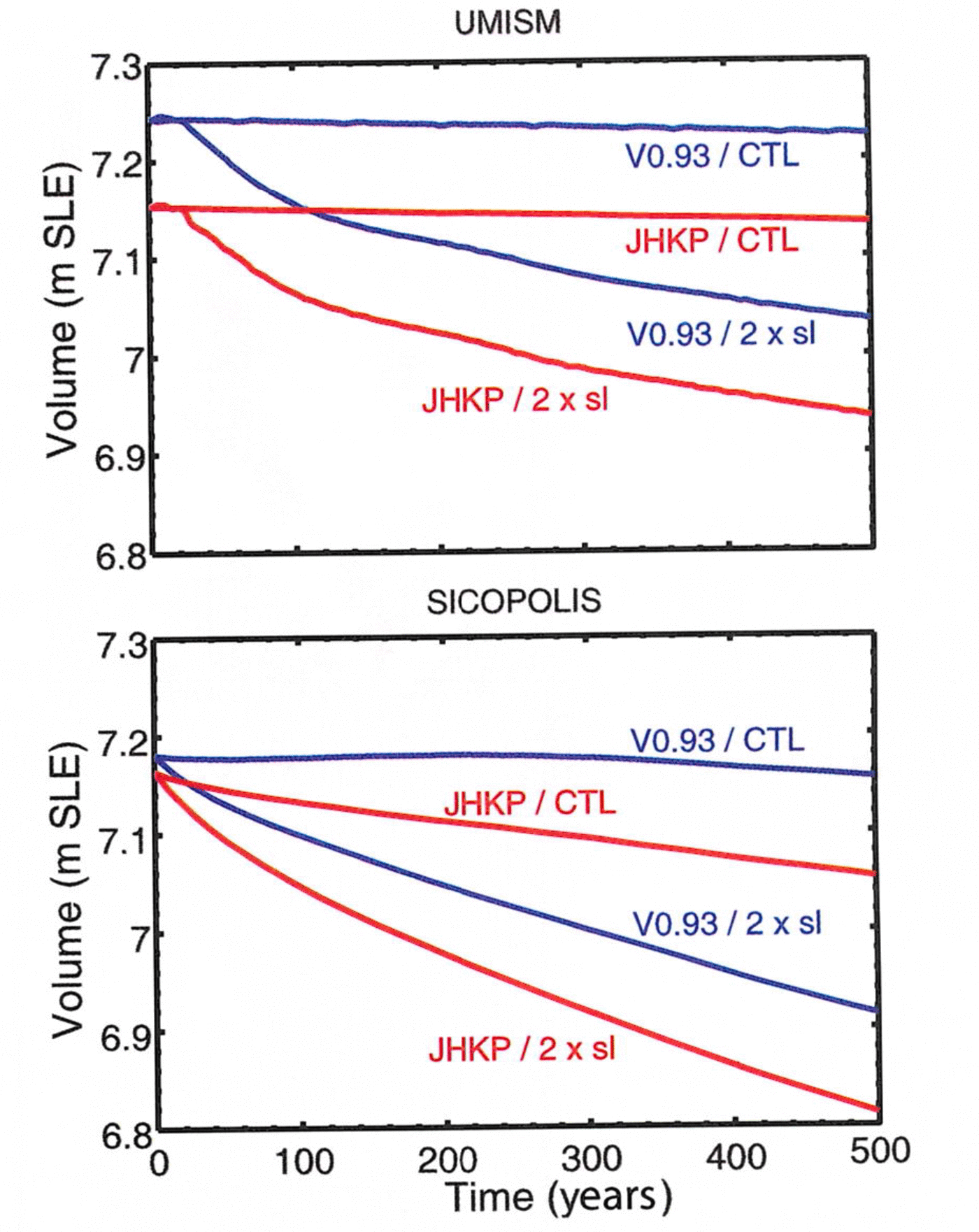
Results of the spin-up runs for the present configuration for the two models are shown in Figures 6 and 7 (UMISM and SICOPOLIS, respectively). Shown here are both surface velocities and basal melt rates or basal water for each of the four modified outlet glaciers. Figure 8 shows the volume of the whole ice sheet, expressed as sea-level equivalent (s.l.e.), calculated for the two different bed representations for a constant-climate control run and a run where sliding was artificially doubled at the end of the spin-up period, run for 500 years into the future. Properties summarized in Section 2.1 are used to validate the model behavior (see also Fig. 1). Results for the whole ice sheet are shown in Figure 9.
Results from UMISM full-spin-up model runs to present. 30 000 year spin-up to present, for bed V0.93 (Reference Bamber, Layberry and GogineniBamber and others, 2001) and for JakHelKanPet bed. Resolution 5 km. Air temperature and precipitation from Reference EttemaEttema and others (2009). (a–d) Jakobshavn Isbræ region; (e–h) Helheim Glacier region; (i–l) Kangerdlussuaq Glacier region; (m–p) Petermann Gletscher region. (a, e, i, m) Ice surface velocity (ma–1) for bed V0.93 (Reference Bamber, Layberry and GogineniBamber and others, 2001). (b, f, j, n) Ice surface velocity (ma–1) for JakHelKanPet bed. (c, g, k, o) Basal water (m) for bed V0.93 (Reference Bamber, Layberry and GogineniBamber and others, 2001). (d, h, l, p) Basal water for JakHelKanPet bed (m). (a–p) Geographic coordinates. (q) Color bar for surface velocity (m a–1). (r) Color bar for thickness of water at bed (m).

Results from SICOPOLIS full-spin-up model runs to present. 125 000 year spin-up to present, for bed V0.93 (Reference Bamber, Layberry and GogineniBamber and others, 2001) and for JakHelKanPet bed. Resolution 5 km. Air temperature from Reference Fausto, Ahlstrøm, Van As, Bøggild and JohnsenFausto and others (2009) and precipitation from Reference EttemaEttema and others (2009). (a–d) Jakobshavn Isbræ region. (e–h) Helheim Glacier region. (i–l) Kangerdlussuaq Glacier region. (m–p) Petermann Gletscher region. (a, e, i, m) Ice surface velocity (m a–1) for bed V0.93 (Reference Bamber, Layberry and GogineniBamber and others, 2001). (b, f, j, n) Ice surface velocity (ma–1) for JakHelKanPet bed. (c, g, k, o) Basal melting rate (ma–1, ice equivalent) for bed V0.93 (Reference Bamber, Layberry and GogineniBamber and others, 2001). (d, h, l, p) Basal melting rate (ma–1, ice equivalent) for JakHelKanPet bed. (a–p) Geographic coordinates. (q) Color bar for surface velocity (ma–1). (r) Color bar for basal melting rate (m a–1, ice equivalent).

Sensitivity of simulated ice-volume change in the next 500 years. Ice volumes (m s.l.e.) as functions of time for both models (UMISM, SICOPOLIS), both beds (V0.93 (Reference Bamber, Layberry and GogineniBamber and others, 2001) and JHKP (JakHelKanPet)), the constant-climate control run 500 years into the future (CTL) and the constant-climate forcing with doubled basal sliding (2×sl). Ice volume is computed as ice volume (m3) times (ice density, 910 kgm–3, divided by sea-water density, 1028 kgm–3) divided by global ocean area (3.61132 × 10¹⁴ m2). The amount of marine ice that does not contribute to sea-level rise is very small for Greenland and thus neglected.
Greenland 5 km subglacial topography and sensitivity of modeled surface velocity. (a) Original bed DEM (Reference Bamber, Layberry and GogineniBamber and others, 2001) (V0.93 in SeaRISE datasets). (b) New JakHelKanPet bed. (a–b) Subglacial elevation in meters above WGS84. Polar stereographic coordinates with central meridian –39.0° E, 90.0° N, latitude of true scale 71.0° N, WGS84 (SeaRISE-type). (c–h) Reconstruction of present-day ice-surface velocity from full spin-ups of ice-dynamic models. Geographic coordinates. (g) Color bar for surface velocity as in Figures 2 and 3 (same color bars used for outlet glaciers and whole-ice-sheet studies). Air temperature by Reference Fausto, Ahlstrøm, Van As, Bøggild and JohnsenFausto and others (2009) and precipitation by Reference EttemaEttema and others (2009) for SICOPOLIS. Air temperature and precipitation by Reference EttemaEttema and others (2009) for UMISM. (c) UMISM, V0.93 bed. (d) UMISM, JHKP bed. (e) SICOPOLIS, V0.93 bed. (f) SICOPOLIS, JHKP bed.

4.1. Present-day surface velocity
UMISM
The velocity structure in Jakobhavn Isbræ shows a vast improvement with the JakHelKanPet bed (Fig. 6 cf. Fig. 1). In runs using the V0.93 bed, the high velocities extend inland to about a quarter of the length of the ice stream, whereas in the JHKP runs, high velocities extend for the correct length of the ice stream (as seen in the crevassed high-velocity areas in Fig. 1), and the southern bend in the South Ice Stream as well as the upper branches are resolved. The spatial acceleration is confined to the margins of the trough, which matches the location of the shear margins (Fig. 1). The averaged bed in V0.93 induces a wide fan of accelerations that extends far beyond the ice stream and the shear margin, especially in the north–south directions.
With the JakHelKanPet bed, the high-velocity areas that define ice streams are now longer, as well as more confined to the trough locations, matching the extent of the crevassed regions indicative of the fast movement of ice streams in satellite imagery and aerial observations (Fig. 1). Differences in bed topography are smaller for Helheim and Kangerdlussuaq Glaciers, since these glaciers already included troughs in the original bed, albeit with lower depths. The effects are similar to those described for Jakobshavn, but not as strong. Velocity patterns align better with crevasse locations indicative of faster flow (Fig. 6 cf. Figs 2 and 3), and areas of accelerated but intermediate velocities occur upstream of the crevassed areas, as expected (Section 2.1).
Petermann Gletscher has a lower overall velocity than the other three glaciers. The match to the present configuration is somewhat problematic, as highest velocities occur where an iceberg broke off the floating tongue, which is not included in the model. Notably, the modeled velocity in the side glaciers of Petermann Gletscher increases. This is an important improvement of the new bed, as the tongue disintegrates over time, and the side glaciers speed up, due to a reduction in buttressing.
In UMISM, highest velocities occur over the floating part of the glaciers, which may be due to the implicit implementation of grounding in this model. Grounding lines are internally defined by the model, when the ice surface drops below the flotation height. In UMISM, grounding-line physics is implemented as a grounding-line element. Each quadrilateral of nodes (points at which bed and other properties are defined and thickness calculated) is examined to see if one or more, but not all, are ice-free with the bed below sea level. Such an element is designated as containing a grounding line, and appropriate grounding-line physics is applied. In particular this includes allowing for an additional thinning rate, meant to accommodate longitudinal extension into the floating ice shelf. This process is controlled by a buttressing parameter, termed the Weertman parameter. This parameter ranges from 1 for no buttressing (full Weertman thinning) to 0 for full buttressing (no thinning). UMISM does not have ice-shelf physics. Hence, wherever velocities are shown, the ice has been calculated as grounded.
A secondary effect of the focusing of high-velocity areas over trough locations is an overall lowering of velocities in neighboring areas (where the bed topography remained unchanged). An example is seen for Storstrømmen at 70° N, north of Jakobshavn, and near Helheim Glacier (Fig. 6); this is an effect of model mathematics. Specifically, basal water is more likely to be focused in the more pronounced Jakobshavn trough than in neighboring areas. Basal water will appear earlier in the deeper channel, providing enhanced flow and lowering the surface. With a lower surface in the trough, the surrounding surface is also lowered, albeit less. With thinner ice, the bed is less likely to become wet and hence might slow down, an effect that is seen in Figure 6b and d. This response of the modeled ice physics to the improved bed topography indicates that all major outlet glaciers should be surveyed and the entire Greenland bed recalculated using the trough-bed algorithm.
Sicopolis
In results of SICOPOLIS runs (Fig. 7), the glacier termini fall within a grid node of the coastline superimposed in the figures (gmt coastline). SICOPOLIS does not include grounding lines explicitly, but ice thickness is forced to be zero along the margin of the ice sheet. Except for this difference, the effect of the new bed JHKP on the model results is similar to that observed for UMISM, but stronger. The region of high velocity for Jakobshavn Isbræ now (i.e. using the JHKP bed) matches the location of the fast ice stream in observations; bends in the ice stream are resolved as well as the upper branches. Somewhat increased velocities fan out over the lower Jakobshavn drainage basin. The effects of increased velocities due to improved bed modeling are strong and widespread for Helheim and Kangerdlussuaq Glaciers.
Discussion of differences in results from the two models
Because of the freely evolving topography applied in the UMISM runs, the ice margin is often too advanced. In the case of Jakobshavn Isbræ, Helheim Glacier and Kangerdlussuaq Glacier, Figure 6 shows that the respective fjords are entirely covered by ice. This is not the case in the SICOPOLIS runs (Fig. 7) where the topography (surface, bed and ice margin) is kept fixed at the measured present-day topography (slightly smoothed), and thus the fjords are largely ice-free. Since the fjords (as opposed to the bedrock troughs further inland) are well represented in both the V0.93 and the JHKP beds, it is not surprising that the UMISM results do not differ much between the two beds.
For Petermann Gletscher the difference between the two beds is quite small (Fig. 5), so both models produce similar results for the two beds. The reason for the poor representation of Petermann Gletscher in SICOPOLIS is that the basal temperature is not at the pressure-melting point in the shallow part of the trough close to the fjord (Fig. 7o and p; no basal melting there) so that fast ice flow cannot develop.
The different basal sliding laws explain why UMISM tends to concentrate fast ice flow more strongly, while fast flow is more distributed for SICOPOLIS. UMISM uses a sliding law that depends on the amount of basal water, which, of course, concentrates in deep troughs. The SICOPOLIS sliding law is independent of basal water and also includes submelt sliding, so basal sliding is smeared out to some extent. UMISM shows ice velocities in Petermann Gletscher in the location where the ice is known to be floating; this may be attributed to the model’s internal calculation of grounding-line positions and the lack of ice-shelf physics.
4.2. Present-day basal melting indicators
Because the basal melting and its control of basal sliding is implemented differently in each model, results can be compared only within and not across the models. However, for both models significant changes in the production of basal water result from the use of the new bed, that indicate a strong sensitivity of that part of the velocity that is due to sliding in the area of newly implemented subglacial trough systems. The geographical distribution of zones of increased basal water production and consequent fast flow for the new bed corresponds to the zones of heavy crevassing (see Fig. 1 for Jakobshavn Isbræ).
UMISM uses the amount of water at the base, defined as equivalent thickness of a volume of water stored at the bed. This may be water in the sediments or water in the ice (similar to the polythermal conditions in SICOPOLIS) but it is probably not a water layer (compare physics of Reference FastookFastook (1993), Reference Fastook and PrenticeFastook and Prentice (1994) and Reference Johnson and FastookJohnson and Fastook (2002) with that of Reference GreveGreve (1995, Reference Greve1997, Reference Greve2005)). Water produced at the bed by basal melting is provided as the source to a model of water transport at the bed. There are several options here, ranging from a conservation-based model that allows for horizontal movement of water to a computationally less expensive 1/e-relaxed point water model. The latter was used in this experiment. All water models calculate the amount of water stored at the bed, expressed as water thickness (m). Water thickness serves as the lubrication factor in the sliding law used in UMISM, so sliding turns on gradually as water amount increases. The amount of water stored at the bed is proportional to the basal melt rate, but it does take time to ‘saturate’ and hence initiate sliding.
For Jakobshavn Isbræ the presence of the deep trough in the new bed topography dramatically increases basal water production from the levels obtained with the original bed. Changes are smaller for Helheim Glacier, because the corrected trough system is less different from the system represented in the old bed and because the trough system is less deep than the Jakobshavn trough.
For SICOPOLIS, Figure 7 shows the basal melting rate (m ice equiv. a–1). In contrast to UMISM, the Weertman-type sliding law used in SICOPOLIS is independent of the amount of basal water. However, water up to a mass fraction of 1% is stored in near-basal layers of temperate ice and increases the flow rate factor there by a factor of up to ~2.8. Any excess water is assumed to be drained instantaneously, thus adding to the basal melting rate but not contributing to basal sliding. This, along with the different ice margin due to the spin-up strategy (Section 2.2), is probably the main reason why the shapes of the simulated ice streams are significantly different between SICOPOLIS and UMISM, and it emphasizes the great importance of basal sliding in ice-stream dynamics.
Independent of the different implementation of basal melting, SICOPOLIS model results also show a significant sensitivity of basal melt rates to bed topography. For Jakobshavn Isbræ, increased basal melting occurs as far inland as the upper reaches of the ice stream. For both Helheim and Kangerdlussuaq Glaciers, the region of increased basal melting coincides with the region of the outlet glacier troughs and a surrounding envelope, which is attributed to an upstream spreading effect of increased sliding. Changes in the basal melt rate for Petermann Gletscher are relatively small, as are changes in bed topography.
4.3. Estimation of future ice-volume loss
To investigate the influence of subglacial topography on ice-sheet evolution, model runs were continued 500 years into the future, once for the V0.93 bed DEM and once for the JKHP bed DEM, following appropriate spin-ups with the same beds and assuming constant climate control and no changes in ice-dynamic principles. Resultant volume loss
from the Greenland ice sheet is shown in Figure 8. Predicted ice-volume loss is ~0.1ms.l.e., larger for model runs using the JHKP bed than for model runs using the V0.93 bed (ice-volume difference 1 at present plus 500 years, ivoldiff1, calculated as

where ivol(500)JHKP,CTL is the ice volume derived for the JHKP bed and ivol(500)V0.93,CTL is the ice volume derived for the V0.93 bed, both at present plus 500 years and under condition CTL (constant climate control)). The evolution of the volume curve is somewhat specific to each model, but the amount of ~0.1ms.l.e. is the same. This is a significant amount of ice-volume loss, so the results from this experiment indicate that topographically and morphologically correct inclusion of outlet glacier troughs in subglacial topography is an important component in modeling ice dynamics and predicting sea-level rise.
A question of interest to the modeling community is how glaciers may respond to increased warming and how this reaction may affect the glacier dynamics. One possibility is that sliding velocity increases. A second experiment was conducted, assuming doubled basal sliding, which is a large change in the physics of a glacier; climate control is again held constant. The doubled-sliding experiment is one of the future-scenario experiments of SeaRISE. (Results of the SeaRISE experiments are reported elsewhere: Reference BindschadlerBindschadler and others (submitted).) Here we investigate the effect of the inclusion of the outlet glaciers in the bed DEM on modeled volume loss and equivalent sea-level rise, assuming an ice dynamics that includes two times the sliding velocity, calculated as ice-volume difference 2

for each ice-sheet model, where 2xsl stands for ‘double-sliding experiment’ and ivol(500)JHKP,2xsl is the ice volume derived for the JHKP bed and ivol(500)V0.93,2xsl the ice volume for the V0.93 bed, both at present plus 500 years. The result (Fig. 8) demonstrates that bed topography remains important in modeling ice dynamics, even if parameters in the ice physics are changed, as may occur in the future. This result is not surprising, considering that morphology and ice flow are two different but interdependent components of the Earth system. For SICOPOLIS, modeled ice volume loss increases faster for the JakHelKanPet bed than for the V0.93 bed. Hence the inclusion of outlet glacier troughs in the Greenland bed topography (or more pronounced outlet glacier troughs, in the case of Helheim and Kangerdlussuaq Glaciers) is relevant for prediction of ice loss.
Comparison of the effects of bed topography and doubled sliding on ice-volume loss using ice-volume difference 3 yields

for UMISM and

for SICOPOLIS, compared to

For SICOPOLIS and UMISM, the doubled sliding of all Greenland glaciers results in approximately twice as much predicted ice-volume loss as the inclusion of the four bed troughs. As doubling sliding everywhere is a large alteration of the physics, but our study includes only four major outlet glaciers, this observation emphasizes the importance of bed topography in predictions of future sea-level rise. A conclusion is that observation of more outlet glaciers and mathematically correct integration of observations into DEMs of subglacial topography is an essential factor in the assessment of sea-level rise.
Defining ice-volume difference 4

and considering the second-order difference

yields that ivoldiff5, the difference in response of the whole ice sheet to doubling of the sliding, dependent on the bed, is an order of magnitude smaller (~0.01 to 0.02 ms.l.e. for the two models) and time-dependent. The quantity ivoldiff5 indicates how much the results of predicted sea-level rise depend on improved bed topography for four glaciers, for the double-sliding experiment and for a fixed time of 500 years.
These calculations indicate that it is of primary relevance to consider the first-order effects in sea-level estimates from existing bed topography (Eqns (1–3)) to understand the physical system. Because the existence of deep troughs increases the acceleration of volume loss over time, prediction experiments are sensitive to bed topography as well, and therefore correct inclusion of troughs reduces the errors on prediction of volume loss and sea-level rise.
5. Discussion and Outlook
The effect on model results from including better bed representations of just four major Greenland glaciers in the bed DEM is significant. The algorithm applied here provides a systematic way to include such features at the lower resolutions currently employed by whole-ice-sheet models. The experiments presented here have been restricted to the four outlet glaciers because of the availability of recently collected data, but as more bed-topographic data are collected as part of NASA’s Operation IceBridge and other geophysical surveys, the bed topography may be updated and improved to include more outlet glaciers.
As computational resources improve, whole-ice-sheet models will be able to run at higher resolution. Increasing spatial resolution of the grid model, at least in the marginal area of the ice sheet, will be necessary to better resolve outlet glaciers. The mathematical-morphological algorithm used to create the JakHelKanPet bed can be applied to generate DEMs of subglacial topography at higher resolution.
Grounding-line determination is problematic in the models. SICOPOLIS does not have a grounding-line concept. UMISM includes grounding-line physics to determine grounding-line positions internally, therefore the improved trough topography may aid in calculations of grounding-line positions. This effect may be worth studying with the help of a higher-resolution DEM and model run. However, given a lack of ice-shelf physics, de facto floating ice may be calculated as grounded ice, especially for glaciers with long floating tongues such as Petermann Gletscher. Similarly, the termini of Kangerdlussuaq and Helheim Glaciers extend to the modern coastline in UMISM model runs, but in reality are located further inland. Investigation of grounding-linephysics is an important topic, but beyond the scope of this paper.
The analyses in this paper demonstrate that with the inclusion of corrected bed DEMs in the four outlet glacier regions, the areas of high velocities agree with the areas of fast flow observed in satellite imagery; or agree much better than for the old bed, with details for each glacier and model discussed in the previous sections. (Areas of fast flow in outlet glaciers are areas of heavy crevassing.) This may motivate a comparison of modeled velocities with observed velocities, which must include analyses of observation technologies, resultant data, analysis methods and related errors on the observation side, and on the modeling side analyses of physical processes included or not included in each model, especially of those processes that interact with topography. For example, UMISM has freely evolving topography whereas SICOPOLIS keeps the topography fixed. The lack of ice-shelf physics affects modeled outlet-glacier velocities, because (1) acceleration propagates up-glacier and (2) an ice shelf causes a back-holding force. Because a modeling/observation comparison has several components, it is left for a follow-up paper.
6. Summary and Conclusions
In summary, model runs using the new JakHelKanPet bed DEM, that includes a morphologically and topographically correct representation of bed troughs of four major ice streams, succeed in reconstructing a realistic spatial distribution of present-day ice-surface velocities and basal meltwater production. High velocities occur in locations matching the crevassed areas indicative of fast glacier movement, and the zones of spatial acceleration are more closely confined to the margins of the ice streams (at the resolution of the models). In contrast, model runs with the old bed DEM (Reference Bamber, Layberry and GogineniBamber and others, 2001) show areas of highest velocities confined to the ice-sheet margin that are broader and too fast over areas far beyond the ice streams. The new bed topography allows the models to more accurately determine where fast flow occurs, especially in UMISM. The spatial distribution and dimensions of basal melt production also improve significantly as a result of using the new bed DEM, with specific changes analogous to those of the surface velocities, which of course are coupled in the models to sliding. Although the two models, UMISM and SICOPOLIS, differ in the physical and numerical implementation of ice dynamics, the improved bed topography has the effect of improving model results (without changing the model physics) in all experiments and both models.
Sensitivity of resultant predictions of (absolute) volume loss from the Greenland ice sheet in the next 500 years is significant, with a change of ~0.1ms.l.e. from inclusion of four major outlet glacier systems. Notably, the amount of ice-volume loss is also on the same order for the two models employed here in experiments assuming (hypothetical) doubled sliding velocities. As comparison of the increase in predicted ice-volume loss from including the four trough systems (~0.1ms.l.e. in the next 500 years) with the effect of hypothetical doubled sliding velocities throughout Greenland (~0.2–0.24ms.l.e. in the next 500 years) indicates, the effect of including (existing) outlet glacier topography is on the same order of magnitude as the effect of assuming a major change in ice dynamics for all Greenland glaciers. These observations demonstrate that topographically and morphologically correct inclusion of outlet glacier troughs in DEMs of subglacial topography is an important component in modeling ice dynamics and predicting sea-level rise. In turn, this requires additional observations of subglacial topography around the margin of the Greenland ice sheets and over outlet glaciers.
The algorithm presented here for generating lower-resolution beds appropriate for whole-ice-sheet models from higher-resolution bed-topography measurements allows the models to more realistically reproduce ice velocities and basal melt production, despite the use of only 5 km grids. The generation of bed DEMs that preserve the shape, orientation and continuity of small-scale geological features, such as the troughs that control the positions of ice streams, is an efficient means of optimally bridging between observations and models.
Acknowledgements
Analysis of CReSIS data and calculation of Greenland bed topography by U.C.H., B.F.W. and B.M. was supported by NASA Cryospheric Sciences Awards NNX09A083G ‘Spatial Ice Surface Roughness – Scale-Dependent Analyses of Ice Surfaces and Implications for Cryospheric Sciences and Satellite Altimetry (in Particular, for ICESat and ICESat-2)’ and NNX11AP39G ‘Spatial Modeling of Greenland Bed Topography as Input for Dynamic Ice Sheet Models: A Contribution to SeaRISE’ (PI U.C. Herzfeld). Assistance with data analysis by P.A.C. and B.M. was supported by the University of Colorado Boulder Undergraduate Research Opportunity Program. R.G.’s SeaRISE modeling studies with SICOPOLIS are funded by a Grant-in-Aid for Scientific Research A (No. 22244058) from the Japan Society for the Promotion of Science (JSPS). J.F. is supported by CReSIS (NSF-ANT-0424589). All this support is gratefully acknowledged. Thanks are also due to Andreas Aschwanden for help with plotting modeling results and discussions of the topic of the paper, to the reviewers and to associate editor Fiamma Straneo.



