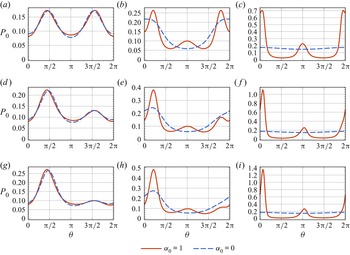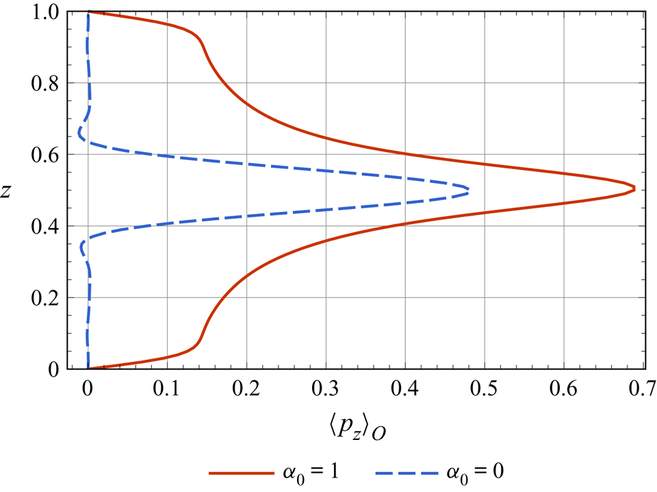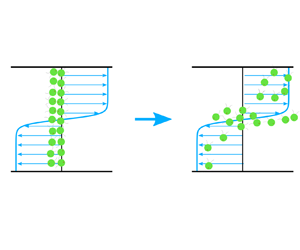

1. Introduction
Thin phytoplankton layers are highly vertically compressed structures of photosynthetic micro-organisms (Durham & Stocker Reference Durham and Stocker2012) as found occasionally in coastal water bodies (Steinbuck et al. Reference Steinbuck, Stacey, McManus, Cheriton and Ryan2009; Penninck et al. Reference Penninck, Lopes, Lima and McManus2020) and stratified lakes (Fee Reference Fee1976; Jones Reference Jones1988; Latasa et al. Reference Latasa, Cabello, Morán, Massana and Scharek2017; Lofton et al. Reference Lofton, Leach, Beisner and Carey2020). Of significant importance to the ecology of aquatic systems, mechanisms underlying the formation, persistence and dissipation of thin phytoplankton layers are hot-spots in marine science (Durham & Stocker Reference Durham and Stocker2012). Several mechanisms have been suggested to be closely related to the formation of thin phytoplankton layers, including an initially high concentration patch straining by shear (Franks Reference Franks1995; Osborn Reference Osborn1998), convergent swimming (Jg, Jj & Ad Reference Jg, Jj and Ad1997; Sullivan, Donaghay & Rines Reference Sullivan, Donaghay and Rines2010) to the sub-surface nutricline, micro-organisms’ autonomous buoyancy-modulating (Walsby Reference Walsby1972) and attaining neutral buoyancy in stratified water columns (Stacey, McManus & Steinbuck Reference Stacey, McManus and Steinbuck2007), gyrotactic trapping of bottom-heavy cells (Durham, Kessler & Stocker Reference Durham, Kessler and Stocker2009; Bearon, Hazel & Thorn Reference Bearon, Hazel and Thorn2011; Ishikawa Reference Ishikawa2012; Ghorai Reference Ghorai2016), in situ growth (Birch, Young & Franks Reference Birch, Young and Franks2008) and intrusions of gravity currents (Kasai et al. Reference Kasai, Kurikawa, Ueno, Robert and Yamashita2010).
In this paper, we concentrate on the gyrotactic trapping mechanism, which was first studied by Durham et al. (Reference Durham, Kessler and Stocker2009) to explain the formation of thin phytoplankton layers in horizontal shear flows. Gyrotactic micro-swimmer is a model of self-propelled particle whose centre of mass is situated in a posterior location than the centre of buoyancy, with respect to the head propelling forward (Pedley & Kessler Reference Pedley and Kessler1992). Many kinds of micro-organisms are gyrotactic, for example, the model organism Chlamydomonas reinhardtii (Karimi & Ardekani Reference Karimi and Ardekani2013) and the harmful alga Heterosigma akashiwo (Bearon, Grünbaum & Cattolico Reference Bearon, Grünbaum and Cattolico2004). In shear flows, the swimming direction of a gyrotactic micro-swimmer is jointly determined by the viscous torque and gravitational torque, if fluid inertia and other random effects are neglected. This process is known as gyrotaxis (Kessler Reference Kessler1985). In a fluid free of shear, gyrotaxis drives the accumulation of cells at the upper surface. Durham et al. (Reference Durham, Kessler and Stocker2009) proposed that, in a strong shear region, the gravitational torque can never compensate the viscous torque exerted by the shear, leading to the disruption of upward migration and gyrotactic trapping.
Although extensive efforts have been made to explore gyrotactic trapping as a possible mechanism for thin phytoplankton layers since the pioneering work of Durham et al. (Reference Durham, Kessler and Stocker2009), obvious inconsistencies remain there between these models. For example, although the results of the continuum model and individual-based model (IBM) are qualitatively comparable in Durham et al. (Reference Durham, Kessler and Stocker2009), there is an inherent difference between the models: the rotational diffusion of micro-organisms is included in their IBM simulation but neglected in their continuum model. In addition, the continuum model they used is associated with a one-dimensional drift–diffusion equation as a preliminary approximation for overall effect, exclusive of other interesting features. A more detailed continuum model was used by Bearon et al. (Reference Bearon, Hazel and Thorn2011): they explored the temporal–spatial distribution of gyrotactic micro-swimmers in flows with variable shear by extending the generalised Taylor dispersion (GTD) theory, which was first proposed by Frankel & Brenner (Reference Frankel and Brenner1989), and applied to gyrotactic micro-organisms in unbounded homogeneous flows by Hill & Bees (Reference Hill and Bees2002) as well as by Manela & Frankel (Reference Manela and Frankel2003). As an illustrating example, they analysed the evolution of gyrotactic micro-swimmers’ vertical concentration distribution, with a vertically uniform line-source release and the same tanh flow profile as the theoretical part of Durham et al. (Reference Durham, Kessler and Stocker2009). However, inconsistent with the explanation of Durham et al. (Reference Durham, Kessler and Stocker2009) for the dissipation of the thin layer that it was due to diffusion, Bearon et al. (Reference Bearon, Hazel and Thorn2011) found that the thin layers disappear in the asymptotic long-time even the flow is laminar and Brownian translational diffusion is neglected; in the meantime, the average up-swimming speed of gyrotactic micro-swimmers is positive at any time and any position, which is consistent with the experimental measurement results of Durham et al. (Reference Durham, Kessler and Stocker2009) (cf. figure 3(B) therein) instead. To explore the persistence of thin layers, Ghorai (Reference Ghorai2016) considered a constant settling speed for the gyrotactic micro-swimmers. Using the same GTD method as Bearon et al. (Reference Bearon, Hazel and Thorn2011) to calculate the effective up-swimming velocity and the vertical diffusivity, the high-dimensional conservation equation was approximated by a one-dimensional drift–diffusion equation. With the settling speed added and the drift–diffusion equation solved, steady thin layers could be found in the tanh flow and in the parabolic flow (the flow velocity profile of the experiment by Durham et al. Reference Durham, Kessler and Stocker2009), even with a finite amount of cells.
Due to the high-dimensional property of the Smoluchowski equation governing the transport of micro-swimmers, solving it directly is resource-consuming (Chen & Jiang Reference Chen and Jiang1999; Saintillan & Shelley Reference Saintillan and Shelley2008). Several models, such as the GTD method and the Pedley–Kessler (P–K) model adopt a drift–diffusion equation in the positional space with two undetermined parameters, namely the drift velocity and the phenomenological diffusion tensor, as mentioned previously. We therefore use ‘two-step GTD method’ to denote the method using a drift–diffusion equation in the positional space with the drift velocity and diffusion tensor determined from GTD theory. To obtain the drift velocity and diffusion tensor, the two-step GTD method used by Bearon et al. (Reference Bearon, Hazel and Thorn2011) and Ghorai (Reference Ghorai2016) is based on an equilibrium hypothesis in the orientational space, making an orientation–position separation possible. Specifically, the two-step GTD method assumed that, after transformation by an operator characterising the fluxes in the orientational space, the shear-dependent quasi-steady orientational distribution of gyrotactic micro-swimmers is equal to zero (see Bearon et al. Reference Bearon, Hazel and Thorn2011, equation (2.10)), and thus the drift velocity can be calculated directly and the diffusion tensor can be obtained with classical GTD theory (Frankel & Brenner Reference Frankel and Brenner1991; Hill & Bees Reference Hill and Bees2002; Manela & Frankel Reference Manela and Frankel2003). The P–K model (Pedley & Kessler Reference Pedley and Kessler1990) is also based on the equilibrium hypothesis and uses the same method to calculate the drift velocity. However, the two-step GTD method predicts a more accurate diffusion tensor than the P–K model (Croze et al. Reference Croze, Sardina, Ahmed, Bees and Brandt2013; Croze, Bearon & Bees Reference Croze, Bearon and Bees2017; Fung, Bearon & Hwang Reference Fung, Bearon and Hwang2020). It should be noted that the equilibrium hypothesis brings three restrictions: ( $1$) the effect of boundary conditions in the orientational–positional space which reflects the interactions between micro-swimmer and boundary should be negligible, because the method was built only for unbounded flows; (
 $2$) the shear variation cannot be too strong, otherwise the assumption of approximating the inhomogeneous shear with locally quasi-homogeneous shear becomes invalid; (
 $3$) the orientational dynamics of the micro-swimmers can be viewed as instantaneous processes compared with positional dynamics. In fact, restrictions (
 $2$) and (
 $3$) often occur simultaneously: because shear variation is a dominant factor in the orientational dynamics, the orientational and positional dynamics of micro-swimmers sampling strongly varying shear cannot be simply separated.
Evidently, the two-step GTD method attempts to solve the drift–diffusion equation in the positional space, with shear-dependent but time-independent drift velocity and diffusion tensor as intermediary parameters. The restriction that two-step GTD model is not accurate for strongly varying shear (Bearon et al. Reference Bearon, Hazel and Thorn2011; Jiang & Chen Reference Jiang and Chen2019, Reference Jiang and Chen2020) can be seen clearly in the comparison with IBM results (Bearon et al. Reference Bearon, Hazel and Thorn2011). Namely there is a ‘breakdown’ parameter region where the micro-swimmers sample rapid-changing shear and thus vitiates the equilibrium hypothesis assumed in the orientational–positional separation. This ‘breakdown’ parameter region exists in the cases of micro-swimmers with strong swimming ability and cases of strongly varying shear. Moreover, the basic understanding of gyrotactic trapping indicates that trapping as a thin layer requires a strong shear region in the flow such as the tanh profile proposed by Durham et al. (Reference Durham, Kessler and Stocker2009), implying that the shear gradient can be very large at the borders of the strong shear layer. As mentioned previously, another assumption of the two-step GTD method is the neglect of the boundary conditions in the orientational–positional space (Bearon et al. Reference Bearon, Hazel and Thorn2011; Jiang & Chen Reference Jiang and Chen2019, Reference Jiang and Chen2020). The boundary conditions therein are often specified as zero-flux or free-stream for the simplified drift–diffusion equation, however, discrepancies can be found between IBM and two-step GTD results when the effect of boundary is influential. For example, Bearon et al. (Reference Bearon, Hazel and Thorn2011) found that, even in Couette flow with homogeneous shear, the two-step GTD method fails to represent the reflective boundary conditions. The boundary effect can be possibly avoided by imposing periodic boundary conditions in some situations (Rusconi, Guasto & Stocker Reference Rusconi, Guasto and Stocker2014; Vennamneni, Nambiar & Subramanian Reference Vennamneni, Nambiar and Subramanian2020), but for practical application, the boundary effect is not always negligible.
As discussed previously, the two-step GTD method is subject to several assumptions and simplifications, posing limitations to a more reasonable understanding of gyrotactic trapping and related micro-swimmers dynamics. An analysis of gyrotactic trapping with an accurate continuum method is still lacking. Actually, for transport in unidirectional flow in the Taylor dispersion regime (asymptotic long-time), the two main drawbacks mentioned previously can be removed by a different choice of local space when applying the GTD theory. With the local space chosen as the orientational coordinate(s) and the bounded positional coordinate(s), and the global space chosen as the streamwise coordinate, Jiang & Chen (Reference Jiang and Chen2019, Reference Jiang and Chen2020) removed the ‘breakdown’ parameter region and satisfactorily handled the effect of boundaries. Long-time asymptotic solution can be obtained with the new GTD method, referred to as ‘one-step GTD method’. For the transient dispersion process, Jiang & Chen (Reference Jiang and Chen2021) derived the time-dependent local moments of probability density function (p.d.f.) of micro-swimmers in the positional–orientational space, by following the expansion of moments derived by Barton (Reference Barton1983) and resorting to the biorthogonal expansion method to the eigenfunctions (Strand, Kim & Karrila Reference Strand, Kim and Karrila1987; Brezinski Reference Brezinski1992).
Using the method in Jiang & Chen (Reference Jiang and Chen2021), i.e. eigenfunction expansion of moments with expansion coefficients determined with the biorthogonal expansion technique, the main purpose of this work is to make an analysis of the transient transport of gyrotactic micro-swimmers in representative simple shear flows. Of special interest to us are the formation, evolution and persistence of the thin layer. To characterise the spatial–temporal transport process, we calculated up to third-order local moments of the p.d.f., which can directly yield the vertical distribution and can be used in the expansion of the positional distribution of the gyrotactic micro-swimmers patch. To accurately investigate the gyrotactic trapping mechanism, the effects of the shear flows, gyrotaxis intensity and swimming ability are characterised. To reflect the fact that some kinds of micro-organisms are negatively buoyant, the effect of settling speed, which is not considered in our previous studies, is investigated with the corresponding boundary conditions tackled.
2. Formulation and solution
2.1. Governing equation
We consider a very dilute suspension of non-interacting point-size micro-swimmers with negligible micro-swimmer-induced hydrodynamic effect. The governing Smoluchowski equation for the conservation of p.d.f. of the micro-swimmers is
 \begin{equation} \frac{\partial P}{\partial t^{{\ast}}}+\boldsymbol{\nabla}_R^{{\ast}} \boldsymbol{\cdot}\boldsymbol{J}_R^{{\ast}}+ \boldsymbol{\nabla}_p\boldsymbol{\cdot} \boldsymbol{j}_p^{{\ast}}=0, \end{equation}
where  $P(\boldsymbol {R},\boldsymbol {p},t^{\ast })$ is the p.d.f. in the orientational-positional space
 $(\boldsymbol {R},\boldsymbol {p})$ at time
 $t^{\ast }$;
 $\boldsymbol {\nabla }_R^{\ast }$ and
 $\boldsymbol {\nabla }_p$ are the gradient operators in the positional space and orientational space, respectively;
 $$\begin{gather} \boldsymbol{J}_R^{{\ast}} = (\boldsymbol{U}^{{\ast}} + V_{s}^{{\ast}} \boldsymbol{p} - V_d^{{\ast}} \boldsymbol{k})P-D_t^{{\ast}} \boldsymbol{\nabla}_R^{{\ast}} P, \end{gather}$$
 $$\begin{gather}\boldsymbol{j}_p^{{\ast}} = \dot{\boldsymbol{p}}^{{\ast}}P-D_r^{{\ast}}\boldsymbol{\nabla}_p P \end{gather}$$
are the p.d.f. fluxes in the positional space and in the orientational space, respectively;  $\boldsymbol {U}^{\ast }$ is velocity of the background flow;
 $V_s^{\ast }$ and
 $V_d^{\ast }$ are the constant swimming speed and settling speed of the micro-swimmers, respectively;
 $\boldsymbol {p}$ and
 $\boldsymbol {k}$ denote the unit vector of a micro-swimmer's orientation and the unit vector opposing the gravity;
 $D_t^{\ast }$ and
 $D_r^{\ast }$ are the Brownian translational diffusivity and rotational diffusivity, respectively;
 $\dot {\boldsymbol {p}}^{\ast }$ is the rate of direction change of the micro-swimmer and is related to the total angular velocity
 $\boldsymbol {\varOmega }_a^{\ast }$ by
 \begin{equation} \dot{\boldsymbol{p}}^{{\ast}}=\boldsymbol{\varOmega}_a^{{\ast}} \times \boldsymbol{p}. \end{equation}
Here  $\boldsymbol {\varOmega }_a^{\ast }$ can be determined by the Jeffery's equation (Jeffery & Filon Reference Jeffery and Filon1922; Hinch & Leal Reference Hinch and Leal1972):
 \begin{equation} \boldsymbol{\varOmega}_a^{{\ast}}=\frac{1}{2B^{{\ast}}}\boldsymbol{p}\times \boldsymbol{k} + \frac{1}{2}{\boldsymbol{\omega}}^{{\ast}}+\alpha_0 [\boldsymbol{p} \times (\boldsymbol{\mathsf{E}}^{{\ast}}\boldsymbol{\cdot} \boldsymbol{p})], \end{equation}
where  $B^{\ast }$ stands for the gyrotactic reorientation time (Pedley & Kessler Reference Pedley and Kessler1987) and micro-swimmer subject to a greater gravitational torque has a larger
 $B^{\ast }$;
 \begin{equation} \boldsymbol{\omega}=\boldsymbol{\nabla}_R^{{\ast}} \times \boldsymbol{U}^{{\ast}} \end{equation}
is the vorticity of the background flow;  $\alpha _0$, ranging from
 $0$ (spherical micro-swimmer) to
 $1$ (rod-like micro-swimmer), is the Bretherton constant (Bretherton Reference Bretherton1962) that characterises the shape anisotropy of the micro-swimmer; and
 $\boldsymbol{\mathsf{E}}^{\ast }$ is the rate-of-strain tensor of the flow,
 \begin{equation} \boldsymbol{\mathsf{E}}^{{\ast}}=\tfrac{1}{2}[\boldsymbol{\nabla}_R^{{\ast}}\boldsymbol{U}^{{\ast}}+(\boldsymbol{\nabla}_R^{{\ast}}\boldsymbol{U}^{{\ast}})^{\mathrm{T}}]. \end{equation}
Note that fluid inertia and particle inertia are neglected in the translational and rotational dynamics of the micro-swimmer, this is justified because we consider the idealised situation with negligible particle Reynolds number  $\textit {Re}_p$ (slip-velocity-induced convective inertia), negligible shear Reynolds number
 $\textit {Re}_s$ (fluid-velocity-gradient-induced convective inertia) and negligible Stokes number
 $St$ (particle inertia), by assuming negligible particle size. The definitions of these dimensionless numbers can be referred to Gustavsson et al. (Reference Gustavsson, Sheikh, Lopez, Naso, Pumir and Mehlig2019).
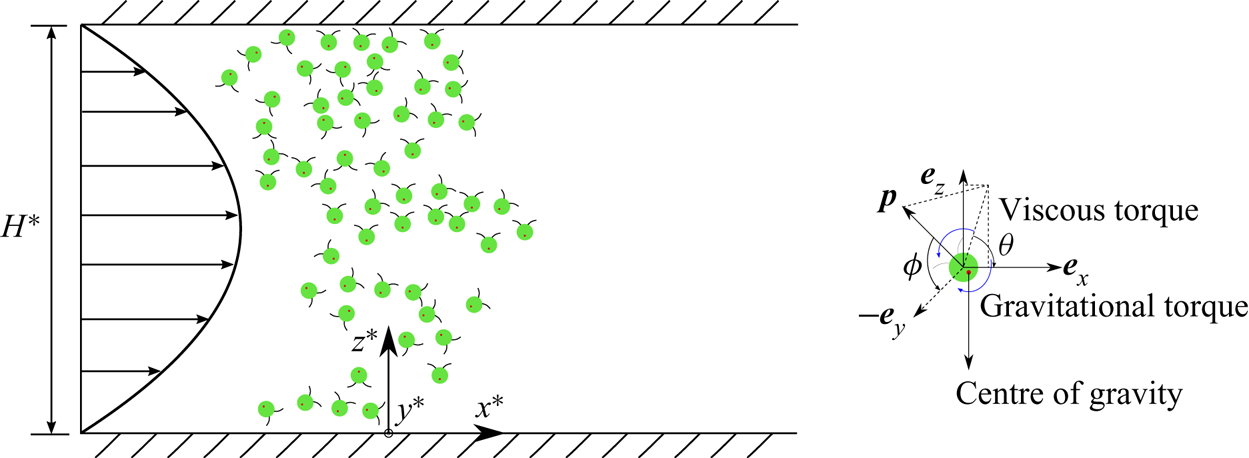
As shown in figure 1, coordinates  $x^{\ast }$ (horizontal axis),
 $y^{\ast }$ (spanwise axis) and
 $z^{\ast }$ (vertical axis) are specified. The associated unit vectors are denoted by
 $\boldsymbol {e}_x$,
 $\boldsymbol {e}_y$ and
 $\boldsymbol {e}_z$. We consider unidirectional flows with vertical shear only, i.e. the flows are homogeneous and unbounded in
 $x^{\ast }$ and
 $y^{\ast }$, thus
 \begin{equation} \boldsymbol{U}^{{\ast}}=U^{{\ast}}(z^{{\ast}})\boldsymbol{e}_x. \end{equation}
Without loss of generality, the motion of micro-swimmers is currently assumed to be three-dimensional (with three positional coordinates and two rotational degrees of freedom). We discuss the simpler situation of two-dimensional micro-swimmers (with two positional coordinates  $x^{\ast }$ and
 $z^{\ast }$ and one rotational degree of freedom) in § 3. We later explore the more general situation of unconstrained rotation (also with two positional coordinates
 $x^{\ast }$ and
 $z^{\ast }$ but two rotational degrees of freedom) in § 4.
A horizontal Poiseuille flow between two infinite parallel plates is chosen to illustrate the problem.  $x^{\ast }$,
 $y^{\ast }$ and
 $z^{\ast }$ are the horizontal, spanwise (into the page) and vertical coordinates, respectively, and
 $(x^{\ast },y^{\ast },z^{\ast })$ make a right-handed Cartesian coordinate. A schematic of a gyrotactic micro-swimmer undergoing Brownian translational and rotational diffusion is shown on the right. Here
 $\phi \in [0,{\rm \pi} )$ is the angle needed to rotate
 $\boldsymbol {p}$ to coincide with
 $-\boldsymbol {e}_y$ and
 $\theta \in [0,2{\rm \pi} )$ denotes the angle formed by the projection of
 $\boldsymbol {p}$ on the
 $x^{\ast }$–
 $z^{\ast }$ plane and
 $\boldsymbol {e}_x$.

Here  $\phi \in [0,{\rm \pi} )$ is defined as the angle needed to rotate
 $\boldsymbol {p}$ to coincide with
 $-\boldsymbol {e}_y$ and
 $\theta \in [0,2{\rm \pi} )$ denotes the angle formed by the projection of
 $\boldsymbol {p}$ on the
 $x^{\ast }$–
 $z^{\ast }$ plane and the positive
 $x^{\ast }$ axis. Note that fixing
 $\phi ={\rm \pi} /2$ corresponds to the situation of two-dimensional micro-swimmers, i.e. constrained rotation. The swimming direction of the micro-swimmer is
 \begin{equation} \boldsymbol{p} = \sin\phi \cos\theta \boldsymbol{e}_x - \cos\phi \boldsymbol{e}_y + \sin\phi \sin\theta \boldsymbol{e}_z. \end{equation}
Dimensionless variables and parameters are specified as
 \begin{align} \left. \begin{array}{c@{}}
\displaystyle t=t^{{\ast}} D_r^{{\ast}}, \quad
x=\dfrac{x^{{\ast}}}{H^{{\ast}}}, \quad
y=\dfrac{y^{{\ast}}}{H^{{\ast}}}, \quad
z=\dfrac{z^{{\ast}}}{H^{{\ast}}}, \quad
U=\dfrac{U^{{\ast}}}{U^{{\ast}}_{max}},\quad
D_t=\dfrac{D_t^{{\ast}}}{D_r^{{\ast}}{H^{{\ast}}}^2},\\
\displaystyle
\textit{Pe}_s=\dfrac{V_s^{{\ast}}}{D_r^{{\ast}}H^{{\ast}}},
\quad
\textit{Pe}_d=\dfrac{V_d^{{\ast}}}{D_r^{{\ast}}H^{{\ast}}},
\quad
\textit{Pe}_f=\dfrac{U^{{\ast}}_{max}}{D_r^{{\ast}}H^{{\ast}}},
\quad \lambda=\dfrac{1}{2B^{{\ast}}D_r^{{\ast}}},
\end{array} \right\} \end{align}
where  $H^{\ast }$ is the depth of the flow and
 $U^{\ast }_{max}$ is the maximum speed of the flow. We note that all flow profiles are modified to be with zero mean velocities before they are non-dimensionalised. Here
 $\textit {Pe}_s$,
 $\textit {Pe}_d$ and
 $\textit {Pe}_f$ are the Péclet numbers characterising the ratios between swimming and rotational diffusion, sedimentation and rotational diffusion, advection and rotational diffusion, respectively;
 $D_t$ reflects the relative strength between Brownian translational diffusion and rotational diffusion;
 $\lambda$ is the dimensionless gyrotactic bias parameter (gyrotaxis intensity).
We assume that the initial release of micro-swimmers is homogeneous in the spanwise  $y$ axis, therefore, no net transport occurs in the
 $y$-direction. The conservation equation (2.1) is recast as
 \begin{equation} \frac{\partial P}{\partial t} ={-} [\textit{Pe}_s \sin\phi \cos\theta + \textit{Pe}_f U(z)] \frac{\partial P}{\partial x} + D_t \frac{\partial ^2 P}{\partial x^2} + \mathcal{L}_u P,\end{equation}
where
 \begin{gather} \mathcal{L}_u({\cdot})=(\textit{Pe}_d-\textit{Pe}_s \sin\phi \sin\theta) \frac{\partial }{\partial z}({\cdot}) + D_t \frac{\partial ^2 }{\partial z^2}({\cdot}) -\frac{\dot{\phi}}{\sin\phi} \frac{\partial }{\partial \phi}({\cdot})-\frac{1}{\sin\phi} \frac{\partial \dot{\phi}}{\partial \phi} ({\cdot}) \nonumber\\ \hspace{0.8pc}+ \frac{1}{\sin \phi} \frac{\partial}{\partial \phi}\left(\sin\phi \frac{\partial }{\partial \phi}({\cdot})\right) - \frac{\partial \dot{\theta}}{\partial \theta}({\cdot})- \dot{\theta}\frac{\partial }{\partial \theta}({\cdot}) + \frac{1}{\sin^2\phi} \frac{\partial ^2 }{\partial \theta^2}({\cdot}), \end{gather}
 $$\begin{gather} \dot{\phi}= \cos\phi \sin\theta \left(\lambda+ \alpha_0 \textit{Pe}_f \frac{\partial U}{\partial z} \sin\phi \cos\theta \right), \end{gather}$$
 $$\begin{gather}\dot{\theta}= \frac{1}{2}\textit{Pe}_f \frac{\partial U}{\partial z}({-}1+\alpha_0 \cos2\theta) + \lambda \csc\phi \cos\theta . \end{gather}$$
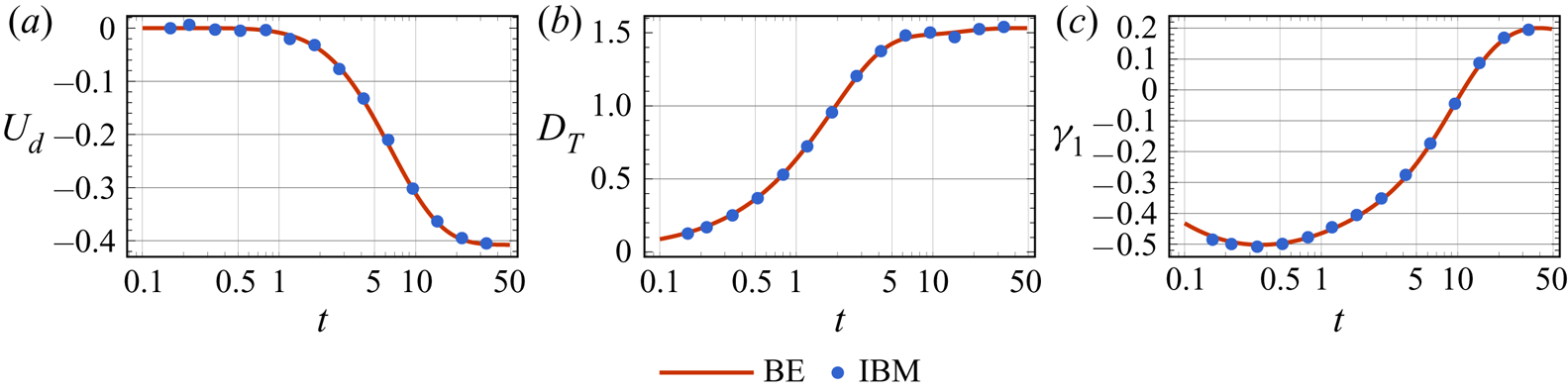
Note that the Smoluchowski equation (2.11) can be equivalently simulated numerically by the IBM (see Appendix A). We use the IBM as a validation of our forthcoming continuum-based method (see e.g. figure 8 for two-dimensional micro-swimmers).
2.2. Boundary conditions and initial condition
With the non-dimensional parameters specified in (2.10),
 \begin{equation} \boldsymbol{J}_R \triangleq \left[\textit{Pe}_f U(z)\boldsymbol{e}_x + \textit{Pe}_s \boldsymbol{p} - \textit{Pe}_d\boldsymbol{e}_z \right] P - D_t \left(\frac{\partial P}{\partial x}\boldsymbol{e}_x + \frac{\partial P}{\partial z}\boldsymbol{e}_z\right) \end{equation}
denotes the non-dimensional positional space flux. As we are concerned about situations with conserved micro-swimmers, no penetration of p.d.f. at the boundaries yields the zero-flux conditions (integral form),
 \begin{align} 0 &=\int^{\rm \pi}_0 \int^{2 {\rm \pi}}_0 \boldsymbol{J}_R \boldsymbol{\cdot} \boldsymbol{e_z} \,\mathrm{d}\theta \,\mathrm{d}\phi \nonumber\\ &=\int^{\rm \pi}_0\int^{2 {\rm \pi}}_0 \left( \textit{Pe}_s \sin\phi \sin \theta P -\textit{Pe}_d P -D_t \frac{\partial P}{\partial z}\right) \mathrm{d}\theta \,\mathrm{d}\phi\quad \mbox{on} \ z=0,1. \end{align}
However, the zero-flux conditions are insufficient to provide enough information for solving the full Smoluchowski equation (2.11) (Ezhilan & Saintillan Reference Ezhilan and Saintillan2015). Instead, they are often implemented in the forms of reflective boundary conditions (Bearon et al. Reference Bearon, Hazel and Thorn2011; Ezhilan, Pahlavan & Saintillan Reference Ezhilan, Pahlavan and Saintillan2012; Jiang & Chen Reference Jiang and Chen2019, Reference Jiang and Chen2020) or Robin boundary conditions (Enculescu & Stark Reference Enculescu and Stark2011; Elgeti & Gompper Reference Elgeti and Gompper2013; Ezhilan & Saintillan Reference Ezhilan and Saintillan2015; Stark Reference Stark2016; Jiang & Chen Reference Jiang and Chen2019, Reference Jiang and Chen2020; Peng & Brady Reference Peng and Brady2020).
We mainly use the reflective boundary conditions in this paper. A discussion for alternative boundary conditions is given in Appendix B. Let  $\theta _0$ denote the incidence angle of the micro-swimmer, we obtain
 $2{\rm \pi} -\theta _0$ for the reflection angle. First, we seek the boundary conditions for
 $P$. The specular reflection treatment in the IBM indicates the following boundary conditions for
 $P$ (Ezhilan et al. Reference Ezhilan, Pahlavan and Saintillan2012; Ezhilan, Alonso-Matilla & Saintillan Reference Ezhilan, Alonso-Matilla and Saintillan2015; Jiang & Chen Reference Jiang and Chen2019):
 \begin{equation} P|_{\theta=\theta_0} = P|_{\theta=2{\rm \pi}-\theta_0} \quad \mbox{on}\ z =0,1,\quad \forall \, \theta_0 \in [0,2{\rm \pi}), \end{equation}
i.e. there is no bias between the p.d.f. of the incidence angle and the p.d.f. of the reflection angle. By symmetry, (2.17) is evident in the absence of flow when one uses the reflective boundary conditions. In the presence of a background flow, because micro-swimmers are reflected instantaneously before the flow takes effect, we expect that the flow does not break the symmetry. It can be also physically interpreted in such a way: if there is a bias in  $\theta _0$ and
 $2{\rm \pi} - \theta _0$ at the boundaries, the reflection treatment, which commutes these two angles, will always eliminate this bias.
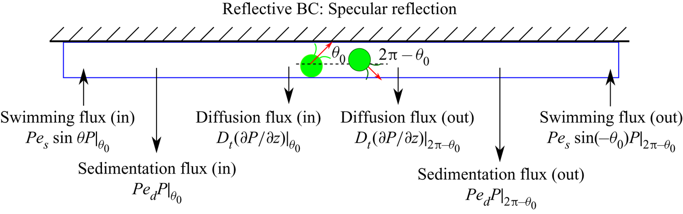
Second, we seek the boundary conditions for the higher-order term  $\partial P/\partial z$. As illustrated in figure 2, viewing from a micro-swimmer's perspective, the balance of positional space flux normal to the boundaries
 $\boldsymbol {J}_R \boldsymbol {\cdot } \boldsymbol {e_z}$ associated with the incidence and the reflection is required:
 \begin{equation} (\boldsymbol{J}_R \boldsymbol{\cdot} \boldsymbol{e_z})|_{\theta=\theta_0} +(\boldsymbol{J}_R \boldsymbol{\cdot} \boldsymbol{e_z})|_{\theta=2{\rm \pi}-\theta_0}=0 \quad \mbox{on}\ z =0,1. \end{equation}
Inserting (2.17) into (2.18) yields
 \begin{align} {-}2\textit{Pe}_d P|_{\theta=\theta_0} - \left. D_t \frac{\partial P}{\partial z}\right|_{\theta=\theta_0} - \left. D_t \frac{\partial P}{\partial z}\right|_{\theta=2{\rm \pi}-\theta_0} =0\quad \mbox{on}\ z =0,1, \quad \forall \, \theta_0 \in [0,2{\rm \pi}) . \end{align}
Illustration of the reflective boundary conditions on the  $x$–
 $z$ plane, corresponding to the specular reflection algorithm in IBM.

For cases without sedimentation, i.e.  $Pe_d=0$, the complete reflective boundary conditions are obtained by combining (2.17) and (2.19) (Jiang & Chen Reference Jiang and Chen2019, Reference Jiang and Chen2020; Wang et al. Reference Wang, Jiang, Chen, Tao and Li2021):
 \begin{equation} \left. \begin{array}{c@{}}
\displaystyle P(x,z,\phi,\theta,t)=
P(x,z,\phi,2{\rm \pi}-\theta,t),\\ \displaystyle \dfrac{\partial
P(x,z,\phi,\theta,t)}{\partial z}={-}\dfrac{\partial
P(x,z,\phi,2{\rm \pi}- \theta,t)}{\partial z}, \end{array}
\right \} \quad \mbox{on}\ z=0,1, \quad \forall \,\theta\in
[0,2{\rm \pi}), \end{equation}
note that the dependence of  $P$ on
 $y$ is dropped.
To perform the biorthogonal expansion and Galerkin method which will be introduced later, one needs to derive corresponding basis functions under the imposed boundary conditions. However, with non-zero settling speed, finding the basis functions directly with (2.19) is potentially difficult. We therefore introduce a transformation to  $P(x,z,\phi,\theta,t)$:
 \begin{equation} P(x,z,\phi,\theta,t)=f_{r}(z) G^r(x,z,\phi,\theta,t), \end{equation}
where
 \begin{equation} f_{r}(z)=\exp\left(-\frac{\textit{Pe}_d}{D_t}z\right). \end{equation}
Notably,  $f_{r}=1$ when the settling speed
 $\textit {Pe}_d$ equals zero. Inserting the transformation (2.21) into the boundary conditions (2.19), we obtain
 \begin{align} 0&={-}f_r \textit{Pe}_d G^r|_{\theta=\theta_0} + f_r \textit{Pe}_d G^r|_{\theta=2{\rm \pi}-\theta_0} - D_t f_r \left.\frac{\partial G^r}{\partial z}\right|_{\theta=\theta_0} - D_t f_r \left.\frac{\partial G^r}{\partial z}\right|_{\theta=2{\rm \pi}-\theta_0}\nonumber\\ &=\left.- D_t f_r \frac{\partial G^r}{\partial z}\right|_{\theta=\theta_0} - \left. D_t f_r \frac{\partial G^r}{\partial z}\right|_{\theta=2{\rm \pi}-\theta_0}. \end{align}
In addition, introducing the transformation (2.21) into the boundary conditions for  $P$ (2.17) and combining (2.23), the boundary conditions with sedimentation can be recovered for
 $G^r$ in the same form as
 $P$ without sedimentation (2.20):
 \begin{equation} \left. \begin{array}{c@{}}
G^r|_{\theta}=G^r|_{2{\rm \pi}-\theta},\\ \displaystyle
\left.\dfrac{\partial G^r}{\partial z}\right|_{\theta}=
\left.-\dfrac{\partial G^r}{\partial
z}\right|_{2{\rm \pi}-\theta}, \end{array} \right \} \quad
\mbox{on}\ z=0,1, \quad \forall \, \theta \in [0,2{\rm \pi}).
\end{equation}
We note that  $D_t$ is important in the fluxes balance at the boundaries, because the neglect of
 $D_t$ leads to a singularity under the Robin boundary conditions and under the reflective boundary conditions with sedimentation. This singular limit has also been discussed in several studies based on continuum approaches (Ezhilan & Saintillan Reference Ezhilan and Saintillan2015; Peng & Brady Reference Peng and Brady2020). Perturbation analysis may be helpful for such a singular limit to address the boundary layer that may develop. In this paper, we do not discuss this singularity and fix
 $D_t=0.01$ unless specifically stated.
The periodic conditions of  $P$ and its derivative are
 \begin{equation} \left.\begin{array}{c@{}} P|_{\theta=0}=P|_{\theta=2{\rm \pi}},\\ \displaystyle \left.\dfrac{\partial P}{\partial \theta}\right|_{\theta=0}= \left.\dfrac{\partial P}{\partial \theta}\right|_{\theta=2{\rm \pi}}, \end{array} \right \} \end{equation}
which also hold for  $G^r$:
 \begin{equation} \left. \begin{array}{c@{}} G^r|_{\theta=0}=G^r|_{\theta=2{\rm \pi}},\\ \displaystyle \left.\dfrac{\partial G^r}{\partial \theta}\right|_{\theta=0}= \left.\dfrac{\partial G^r}{\partial \theta}\right|_{\theta=2{\rm \pi}}. \end{array} \right \} \end{equation}
The boundary conditions (2.24) and the periodic conditions (2.26) admit a concise basis for  $G^r$, namely reflective basis (denoted by
 $\{g_i^r\}_{i=1}^{\infty }$). The basis functions are derived with the Laplace operator on the local space
 $(z,\phi,\theta )$
 \begin{equation} \varDelta_q = \frac{\partial}{\partial z^2} + \frac{1}{\sin \phi} \frac{\partial}{\partial \phi} \left(\sin\phi \frac{\partial}{\partial \phi}\right) + \frac{1}{\sin^2 \phi} \frac{\partial^2}{\partial \theta^2}, \end{equation}
with the corresponding inner product
 \begin{equation} (f,g) \triangleq \int_0^1 \int_0^{2{\rm \pi}} \int_0^{\rm \pi} f(z,\phi,\theta) g(z,\phi,\theta) \sin\phi\,\text{d}\phi \,\text{d}\theta \,\text{d}z. \end{equation}
One can verify that  $\varDelta _q$ is self-adjoint under the boundary conditions (2.20) or (2.24).
The eigenfunctions of  $\varDelta _q$ are
 \begin{equation} \left. \begin{array}{c@{}}
\displaystyle N_n \sqrt{\dfrac{2l+1}{4{\rm \pi}}} \cos(n {\rm \pi}z)
{P}_l (\cos\phi), \\ \displaystyle N_n
\sqrt{\dfrac{2l+1}{2{\rm \pi}} \dfrac{(l-m)!}{(l+m)!}} \cos(n {\rm \pi}
z) \cos(m\theta) {P}_l^m (\cos\phi), \\ \displaystyle N_n
\sqrt{\dfrac{2l+1}{2{\rm \pi}} \dfrac{(l-m)!}{(l+m)!}} \sin(n {\rm \pi}
z) \sin(m\theta) {P}_l^m (\cos\phi), \end{array} \right \}
\end{equation}
where  $m=1,2,\ldots, l$;
 $l=0,1,2,\ldots$;
 $n=0,1,2,\ldots$;
 \begin{equation} N_n = \begin{cases} 1, & n=0, \\ \sqrt{2}, & n>0; \end{cases} \end{equation}
is the normalisation factor;  ${P}_l$ and
 ${P}_l^m$ are the Legendre polynomials of degree
 $l$ and associated Legendre polynomials of degree
 $l$ and order
 $m$, respectively. We note that, because
 $P(x,z,\phi,\theta,t)$ is symmetric to the transformation
 \begin{equation} \phi\to {\rm \pi}- \phi, \end{equation}
we can therefore drop basis functions that are not symmetric about  $\phi ={\rm \pi} /2$ in the calculation.
For the situation of two-dimensional micro-swimmers (constrained rotation), the basis simplifies to
 \begin{equation} \left.\begin{array}{c@{}} \dfrac{1}{\sqrt{2{\rm \pi}}},\quad \dfrac{1}{\sqrt{\rm \pi}} \cos (n {\rm \pi}z), \quad \dfrac{1}{\sqrt{\rm \pi}}\cos (m \theta),\\ \sqrt{\dfrac{2}{\rm \pi}}\cos (n {\rm \pi}z)\cos (m \theta) ,\quad \sqrt{\dfrac{2}{\rm \pi}}\sin (n {\rm \pi}z) \sin (m \theta), \end{array} \right \} \end{equation}
where  $m = 1, 2, \ldots$,
 $n = 1, 2, \ldots$.
When investigating the asymptotic long-time solutions (Jiang & Chen Reference Jiang and Chen2019, Reference Jiang and Chen2020), a special form of the initial condition is not required, because the long-time asymptotic dispersion coefficients (such as streamwise-averaged vertical distribution, drift and dispersivity) are unaffected by it. In this paper, because we are concerned about transient dynamics, the initial condition is formally given as
 \begin{equation} P(x,z,\phi,\theta,0)=\displaystyle \delta(x) P_{ic}(z,\phi,\theta), \end{equation}
where  $\delta$ is the Dirac delta function. Unless stated specifically, we assume that the micro-swimmers are uniformly released in the
 $z$-direction (vertically uniform line-source release) with the initial orientation uniformly distributed in the
 $x$–
 $z$ plane, thus
 \begin{equation} P_{ic}(z,\phi,\theta)= \frac{1}{2{\rm \pi}}\delta\left (\phi-\frac{\rm \pi}{2}\right). \end{equation}
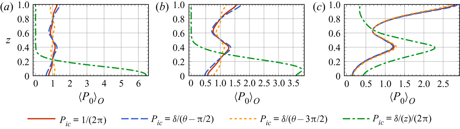
It is noteworthy that one drawback of the two-step GTD method is that it cannot reflect the initial orientational distribution of the micro-swimmers. We give a discussion on different initial conditions in Appendix C, where micro-swimmers do not have uniformly distributed orientations or vertical positions when they are released.
As we are considering a finite amount of micro-swimmers injected in a limited range, the following classical conditions can be imposed
 \begin{equation} \left. \begin{array}{ll@{}} P \to 0 & \mbox{as}\ |x|\to \infty,\\ \displaystyle \dfrac{\partial P}{\partial x} \to 0 & \mbox{as}\ |x| \to \infty, \end{array} \right \} \end{equation}
which will be used in deriving the governing equation of moments (Aris Reference Aris1956; Chatwin Reference Chatwin1970; Guan et al. Reference Guan, Zeng, Li, Guo, Wu and Wang2020; Wu et al. Reference Wu, Singh, Foufoula-Georgiou, Guala, Fu and Wang2021).
2.3. Governing equation and boundary conditions of local moments
The local moments of p.d.f. are defined as (Aris Reference Aris1956; Wu & Chen Reference Wu and Chen2015)
 \begin{equation} P_n(z,\phi,\theta,t)\triangleq \int_{-\infty}^{\infty} x^n P(x,z,\phi,\theta,t) \, \mathrm{d}\kern0.7pt x,\quad n=0,1,\ldots, \end{equation}
thus  $P_0(z,\phi,\theta,t)$ is the time-dependent distribution in the local space (
 $z,\phi,\theta$). The vertical distribution
 $\langle P_0 \rangle _{O}(z,t)$ is obtained by integrating the zeroth local moment
 $P_0(z,\phi,\theta,t)$ in the orientational space
 $(\phi,\theta )$
 \begin{equation} \langle P_0 \rangle_{O} (z,t)= \int_0^{\rm \pi} \int_0^{2{\rm \pi}} P_0(z,\phi,\theta,t)\, \mathrm{d}\theta \, \mathrm{d}\phi. \end{equation}
With the aid of (2.35), governing equations of  $P_0$,
 $P_1$ and
 $P_2$ can be obtained by multiplying (2.11) and integrating with respect to
 $x \in (-\infty,\infty )$:
 $$\begin{gather} \frac{\partial P_0}{\partial t} = \mathcal{L}_u P_0, \end{gather}$$
 $$\begin{gather}\frac{\partial P_1}{\partial t} = (\textit{Pe}_f U + \textit{Pe}_s \sin\phi \cos\theta)P_0 + \mathcal{L}_u P_1, \end{gather}$$
 $$\begin{gather}\frac{\partial P_2}{\partial t} = 2D_tP_0 + 2(\textit{Pe}_f U + \textit{Pe}_s \sin\phi \cos\theta)P_1 + \mathcal{L}_u P_2. \end{gather}$$
Note that, for cases only considering the transport in the vertical direction (e.g. Ghorai Reference Ghorai2016), i.e. by assuming the initial condition is homogeneous in the  $x$-direction, the governing equation of the p.d.f. is the same as (2.38).
With the same transformation (2.21) to  $P$,
 $P_n$ (
 $n=0,1,2$) is decomposed as
 \begin{equation} P_n=f_r G^r_n. \end{equation}
We note that the boundary conditions (2.19) for  $P$ also hold for
 $P_n$, which means
 $G^r$ and
 $G_n^r$ share the same basis functions.
We define a new operator  $\mathcal {L}_r(\cdot )$ satisfying
 $\mathcal {L}_r G_n^r = (\mathcal {L}_u P_n)/f_r$, and its relation to
 $\mathcal {L}_u (\cdot )$ is
 \begin{equation} \mathcal{L}_r({\cdot}) \triangleq \mathcal{L}_u ({\cdot}) - 2 \textit{Pe}_d \frac{\partial}{\partial z}({\cdot}) + \frac{1}{D_t} \textit{Pe}_d \textit{Pe}_s \sin\phi \sin\theta ({\cdot}), \end{equation}
such that  $G^r_n$ satisfies
 \begin{equation} \frac{\partial G^r_n}{\partial t} = n(n-1)D_tG^r_{n-2}+ n[\textit{Pe}_f U(z) + \textit{Pe}_s \sin\phi \cos\theta]G^r_{n-1} + \mathcal{L}_rG^r_n,\quad n=0,1,\ldots. \end{equation}
2.4. Eigenfunction expansion of local moments
Following Barton (Reference Barton1983) and Jiang & Chen (Reference Jiang and Chen2021), we write the transformed local moments  $G_n^r$ in the form of eigenfunction expansion:
 \begin{equation} G_n^r(z,\phi,\theta,t)=\sum_{i=1}^{\infty} p_{ni}(t) \mathrm{e}^{-\lambda_i t} f_i(z,\phi,\theta), \quad n=0,1,\ldots, \end{equation}
where  $-\lambda_i$ and
 $f_i$ are the eigenvalues and eigenfunctions of operator
 $\mathcal {L}_r$ with
 $\lambda _i$ sorted in an ascending order. Here
 $p_{ni}$ are the undetermined expansion coefficients,
 $\lambda _1=0$ and the corresponding eigenfunction
 $f_1$ characterises the steady state, which has been discussed in Jiang & Chen (Reference Jiang and Chen2019, Reference Jiang and Chen2020) and Wang et al. (Reference Wang, Jiang, Chen, Tao and Li2021).
The eigenvalue problem of  $\mathcal {L}_r$ is
 \begin{equation} \mathcal{L}_r f_i=-\lambda_i f_i, \end{equation}
however, this eigenvalue problem cannot be easily solved due to the complexity of the operator  $\mathcal {L}_r$. Following Jiang & Chen (Reference Jiang and Chen2021), we approximate the solution with a Galerkin method. With the basis functions
 $\{g_i^r\}_{i=1}^{\infty }$ given in (2.29),
 $f_i$ can be expanded as
 \begin{equation} f_i=\sum_{j=1}^{\infty}\phi_{ij}g_j^r, \end{equation}
where  $\phi _{ij}$ are the coefficients. A bilinear form
 $A$ is defined as
 \begin{equation} A(g_i^r,g_j^r)=\langle g_i^r,\mathcal{L} g_j^r \rangle =\int_0^1 \int_0^{2{\rm \pi}} \int_0^{\rm \pi} g_i^r\cdot(\mathcal{L} g_j^r) \, \mathrm{d}\phi \, \mathrm{d}\theta \, \mathrm{d} z. \end{equation}
With  $g_i$ truncated at a degree M and
 $f_i$ truncated at a degree
 $N$, the weak form of the eigenvalue problem (2.45) can then be written in a matrix form:
 \begin{equation} \boldsymbol{\mathsf{A}} \boldsymbol{\phi_i} = \lambda_i \boldsymbol{\phi_i}, \end{equation}
where  $\boldsymbol{\mathsf{A}}_{ij}=A(g_i^r,g_j^r)$ and
 $\boldsymbol {\phi _i}=(\phi _{i1},\phi _{i2},\ldots,\phi _{iN})^{\mathrm {T}}$.
2.5. Biorthogonal expansion of moments
If  $\{f_i\}_{i=1}^N$ are orthogonal, then the procedure for solving
 $P_n$ can be readily done by inserting (2.44) into (2.43) and integrating over the cross-section to obtain
 $\{p_{ni}\}_{i=1}^{N}$, as is often the case in studying passive tracer transport (Barton Reference Barton1983; Wang & Chen Reference Wang and Chen2017b; Guo et al. Reference Guo, Jiang, Zhang, Li and Chen2019). However, in the current situation,
 $\{f_i\}_{i=1}^N$ are not orthogonal because
 $\mathcal {L}_r$ is not self-adjoint. Jiang & Chen (Reference Jiang and Chen2021) used another set of eigenfunctions, namely the dual basis functions
 $\{f_i^{\star }\}_{i=1}^N$ satisfying the biorthogonality relation with
 $\{f_i\}_{i=1}^N$ if both are normalised (Strand et al. Reference Strand, Kim and Karrila1987; Brezinski Reference Brezinski1992)
 \begin{equation} \langle f_i^{{\star}},f_j\rangle =\delta_{ij}, \end{equation}
where  $\delta _{ij}$ is the Kronecker delta. Therefore,
 $\{f_i^{\star }\}_{i=1}^N$ can be used to determine the expansion coefficients
 $\{p_{ni}\}_{i=1}^{N}$.
The dual basis functions  $\{f_i^{\star }\}_{i=1}^N$ are the eigenfunctions of the adjoint operator of
 $\mathcal {L}_r$ and is expressed as
 \begin{align*} f_i^{\star} = \sum_{j=1}^{\infty} \phi_{ij}^{\star} g_j^r\end{align*}
The Galerkin method is again used to solve this eigenvalue problem. Let  $\boldsymbol{\mathsf{A}}^{\star }$ denote the corresponding matrix, then
 \begin{equation} \boldsymbol{\mathsf{A}}^{{\star}} \boldsymbol{\phi_i}^{{\star}} = \lambda_i \boldsymbol{\phi_i}^{{\star}}, \end{equation}
where  $\boldsymbol {\phi }_{i}^{\star }=(\phi _{i1}^{\star },\phi _{i2}^{\star },\ldots,\phi _{iN}^{\star })^{\mathrm {T}}$. Note that
 $\boldsymbol{\mathsf{A}}^{\star }=\boldsymbol{\mathsf{A}}^{\mathrm {T}}$. With the dual basis functions
 $\{f_i^{\star }\}_{i=1}^N$ obtained,
 $\{p_{ni}\}_{i=1}^{N}$ can be solved using the biorthogonality relation.
We test the convergence to graphical accuracy of the steady distribution  $\langle P_0\rangle _{{O}}^{\infty }$ by directly solving the boundary value problem
 $\mathcal {L}_r G_0= 0$ with different total numbers of basis functions. For the situation of two-dimensional micro-swimmers, we truncate
 $n=60$ for the vertical direction and
 $m=15$ for the orientational space in most cases, as including more basis functions (
 $n=120, m=30$) does not change the results. For settling micro-swimmers in the tanh flow with
 $\textit {Pe}_f=10$ and
 $\textit {Pe}_s=1$, the convergence is attained at
 $n=120$, this is probably due to the double peaks of the concentration profile (see e.g. figure 10d).
For the situation of unconstrained rotation, we truncate  $n=60$ for the vertical direction and
 $l=15$ for the orientational space, since the solutions in each case are found to be identical to those with a higher resolution (
 $n=100,\ l=30$). Details of obtaining the solution with a Galerkin method and Legendre polynomial basis are similar to Jiang & Chen (Reference Jiang and Chen2020, Appendix A).
A convergence is also tested for  $N$ (the total numbers of eigenfunctions used in the expansion of local moments (2.44)), and we use
 $N=40$ for all cases. Some higher-order quantities obtained with the biorthogonal expansion and the IBM are compared in Appendix A. Other validations of vertical distribution
 $\langle P_0\rangle _{O}$ are shown in figures 8, 15 and 17.
3. Gyrotactic trapping of two-dimensional micro-swimmers
We first explore the fundamentals of gyrotactic trapping by considering two-dimensional micro-swimmers, i.e. constrained rotation (fix  $\phi ={\rm \pi} /2$). We focus on spherical micro-swimmers, i.e.
 $\alpha _0=0$ in (2.5). We also discuss cases with non-settling rod-like (
 $\alpha _0=1$) micro-swimmers in Appendix D. However, cases with settling elongated micro-swimmers is not discussed in this paper, because the settling speed will become orientation-dependent (Ardekani et al. Reference Ardekani, Sardina, Brandt, Karp-Boss, Bearon and Variano2017; Clifton, Bearon & Bees Reference Clifton, Bearon and Bees2018), and the possible inertial torque can be a non-negligible effect (Lopez & Guazzelli Reference Lopez and Guazzelli2017; Gustavsson et al. Reference Gustavsson, Sheikh, Lopez, Naso, Pumir and Mehlig2019; Sheikh et al. Reference Sheikh, Gustavsson, Lopez, Lévêque, Mehlig, Pumir and Naso2020; Qiu et al. Reference Qiu, Cui, Climent and Zhao2021; Wang, Jiang & Chen Reference Wang, Jiang and Chen2022).
3.1. Plane Poiseuille flow
We first investigate the transport of gyrotactic micro-swimmers in the plane Poiseuille flow. The evolution of cell concentration in this configuration was also studied by Ishikawa (Reference Ishikawa2012) with Stokesian dynamics-based simulations. In his investigation, transient layers of high concentration occurred in cases with strong flow (large  $\textit {Pe}_f$) and weak gyrotaxis (small
 $\lambda$). In this subsection, we study this process by altering the micro-swimmers’ swimming ability (quantified by
 $\textit {Pe}_s$) and gyrotactic bias (quantified by
 $\lambda$) as well as shear strength (quantified by
 $\textit {Pe}_f$). The dimensionless velocity profile of the plane Poiseuille flow is
 \begin{equation} U(z)=12z(1-z)-2. \end{equation}
3.1.1. Non-settling micro-swimmers
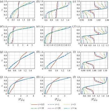
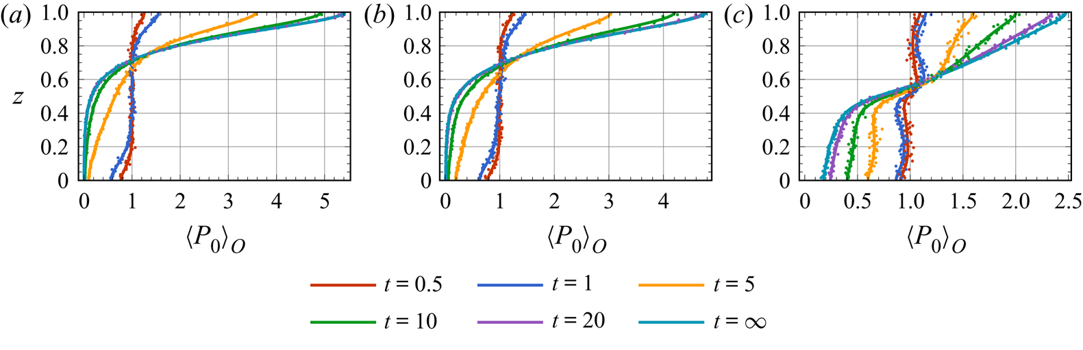
As shown in figure 3, the vertical distributions of line-source-released gyrotactic micro-swimmers are depicted at the sample times  $t\in \{0.5, 1, 5, 10, 20\}$ and the final steady state
 $t=\infty$ (which is calculated by solving the boundary value problem
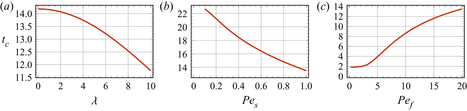
 $\mathcal {L}_u P_0(z,\theta ) = 0$ directly). First, we see that the relaxation time to the steady state varies with cases: the relaxation time increases with increasing
 $\textit {Pe}_f$,
 $1/\textit {Pe}_s$ or
 $1/\lambda$, i.e. strong overall shear, weak swimming ability and weak gyrotaxis can extend the time required to reach the steady state. Inspection of the explicit expression of the zeroth local moment
 $P_0(z,t)$ (Jiang & Chen Reference Jiang and Chen2021, Appendix A) shows that the all the expansion coefficients
 $p_{0i}$ in (2.44) are constant. Therefore, the relaxation time to the steady state can be roughly evaluated by the second (the smallest non-zero) eigenvalue
 $\lambda _2$ of the expansion (2.44) (Aris Reference Aris1956). Let
 $t_c$ denote the time required for
 $\mathrm {e}^{\lambda _2 t}$ to decay from
 $1$ to
 $0.1$, the variations of
 $t_c$ as functions of
 $\lambda$,
 $\textit {Pe}_s$ and
 $\textit {Pe}_f$ are plotted in figure 4.
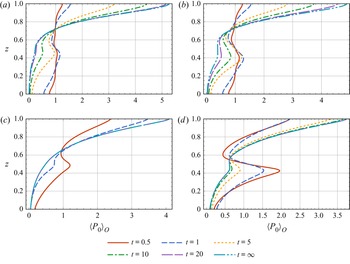
Transient vertical distributions  $\langle P_0 \rangle _{O}$ of a vertically uniform line-source release of non-settling gyrotactic micro-swimmers in the plane Poiseuille flow: (a)–(c)
 $\textit {Pe}_s=0.1$,
 $\lambda =1$; (d)–(f)
 $\textit {Pe}_s=0.1$,
 $\lambda =5$; (g)–(i)
 $\textit {Pe}_s=1$,
 $\lambda =1$; (j)–(l)
 $\textit {Pe}_s=1$,
 $\lambda =5$; (a), (d), (g), (j)
 $\textit {Pe}_f=0.1$; (b), (e), (h), (k)
 $\textit {Pe}_f=1$; (c), (f), (i), (l)
 $\textit {Pe}_f=10$. Common parameters:
 $\textit {Pe}_d=0$,
 $D_t=0.01$.

Time duration  $t_c$ for
 $\mathrm {e}^{\lambda _2 t}$ to decay from
 $1$ to
 $0.1$: (a)
 $\textit {Pe}_f=10$,
 $\textit {Pe}_s=1$; (b)
 $\textit {Pe}_f=10$,
 $\lambda =5$; (c)
 $\textit {Pe}_s=1$,
 $\lambda =5$. Common parameters:
 $\textit {Pe}_d=0$,
 $D_t=0.01$.

Qualitatively consistent with the results of Ishikawa (Reference Ishikawa2012), transient layers of high concentration can be found in cases with strong overall shear, as shown in figure 3(c), 3( f), 3(i) and 3(l). In other cases with weak shear, in contrast, the gyrotactic micro-swimmers quickly accumulate at the upper boundary instead of being trapped in the bulk. This phenomenon can be understood by considering the competing effects between gyrotaxis-driven up-swimming and the rapid unbiased rotation of the local shear, forming the basic concept of gyrotactic trapping. As in the plane Poiseuille flow, the rate of shear increases linearly from the centre to the boundaries, thus the gyrotactic micro-swimmers experience weaker up-swimming resistance in the centre region. Namely, the gyrotactic micro-swimmers can easily migrate from the lower half of the centre region ( $z\approx 0.4$) to the upper half of the centre region (
 $z\approx 0.6$), but the subsequent migration can be inhibited by the shear, leading to a layer of high concentration at the upper half of the centre region. In addition, the gyrotactically trapped layer at the upper half favours larger
 $\textit {Pe}_s$ and this is attributed to a larger upward migration flux gradient, which counteracts the diffusion effect homogenising the concentration.
The gyrotactic trapping mechanism can be captured more clearly by considering governing equation for the vertical distribution  $\langle P_0\rangle _{{O}}$, which can be obtained by integrating (2.38) with respect to
 $\theta \in [0,2{\rm \pi} )$:
 \begin{align} \frac{\partial{\langle P_0 \rangle_{O}}}{\partial t} &={-}\frac{\partial J_z}{\partial z}+D_t\frac{\partial ^2 \langle P_0\rangle_{{O}}}{\partial z^2} \nonumber\\ &={-}\textit{Pe}_s \langle p_z \rangle_{{O}} \frac{\partial \langle P_0 \rangle_{{O}}}{\partial z} - \textit{Pe}_s \langle P_0 \rangle_{{O}} \frac{\partial \langle p_z\rangle_{{O}}}{\partial z} + D_t \frac{\partial^2 \langle P_0 \rangle_{{O}}}{\partial z^2}, \end{align}
where
 \begin{equation} J_z(z,t)= \textit{Pe}_s \langle P_0\rangle_{{O}} \langle p_z\rangle_{O} \end{equation}
is the up-swimming flux of the micro-swimmers patch, and
 \begin{equation} \langle p_z \rangle_{O}(z,t) = \frac{\displaystyle\int_0^{2{\rm \pi}} P_0 \sin \theta \, \text{d}\theta}{\displaystyle\int_0^{2{\rm \pi}} P_0 \, \text{d}\theta} \end{equation}
is the mean up-swimming orientation component.
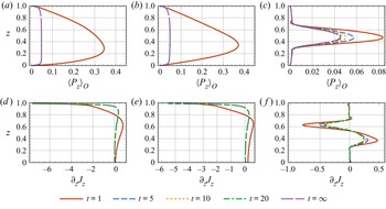
The evolution of mean up-swimming orientation component  $\langle p_z \rangle _{O}$ and up-swimming flux gradient
 $\partial J_z/\partial z$ is plotted in figure 5. We can see that, for all sampled time ticks in cases with strong overall shear (figure 5c),
 $\langle p_z \rangle _{O}$ is wedge-like peaking at
 $z=0.5$, where the local shear is the weakest. Therefore, the up-swimming flux
 $\textit {Pe}_s \langle p_z \rangle _{O}$ is the largest. In addition, the up-swimming flux gradient
 $\partial J_z/\partial z$ reaches its minimum around
 $z=0.6$, resulting in a high concentration layer. However, in weak flows,
 $\langle p_z \rangle _{O}$ is more like a trapezoid, as depicted in figure 5(a) and 5(b). In addition, in figure 5(d) and 5(e), we see that the up-swimming flux gradient
 $\partial J_z/\partial z$ decreases monotonically as
 $z$ approaches
 $1$ after attaining its maximum, indicating a strong gravitactic focusing at the upper boundary instead of gyrotactic trapping in the bulk.
Transient mean up-swimming orientation component  $\langle p_z \rangle _{O}$ and up-swimming flux gradient
 $\partial _z J_z$ of a vertically uniform line-source release of non-settling gyrotactic micro-swimmers in the plane Poiseuille flow: (a), (d)
 $\textit {Pe}_f=0.1$; (b), (e)
 $\textit {Pe}_f=1$; (c), (f)
 $\textit {Pe}_f=10$. For
 $\textit {Pe}_f=0.1$ and
 $1$, lines with
 $t \geq 5$ are indistinguishable. Common parameters:
 $\textit {Pe}_s=1$,
 $\textit {Pe}_d=0$,
 $\lambda =5$,
 $D_t=0.01$.

Notably, we can see that  $\langle p_z \rangle _{O}$ is both
 $z$-dependent (shear-dependent) and
 $t$-dependent in figure 5. The shear-dependent feature can be understood by considering the variable rate of local shear which rotates the micro-swimmer either faster or slower. Strong local shear leads to weak up-swimming and weak local shear leads to strong up-swimming. The
 $t$-dependent feature actually signifies the effect of initial orientational distribution and the effect of boundaries, both of which are not considered in the two-step GTD method based on the local equilibrium hypothesis.
One advantage of solving the successive local moments  $P_n(z,\theta,t)$ is that they contain important statics of the micro-swimmers patch which cannot be obtained by assuming an initially homogeneous p.d.f. in the
 $x$-direction. With the local moments
 $P_n(z,\theta,t)$ integrated over
 $\theta \in [0,2{\rm \pi} )$, namely
 $\langle P_n \rangle _{{O}}(z,t)$, one can expand the two-dimensional time-dependent concentration
 $\langle P \rangle _{O} (x,z,t)$ in the series of Hermite polynomials. For example, given the moments, Gram–Charlier Type A series (Kendall & Stuart Reference Kendall and Stuart1958; Blinnikov & Moessner Reference Blinnikov and Moessner1998) and its Edgeworth form (Chatwin Reference Chatwin1970) are widely used in ‘reconstructing’ the cross-sectional-averaged concentration in the streamwise direction (Chatwin Reference Chatwin1970; Wang & Chen Reference Wang and Chen2017a) and full positional concentration field (Li et al. Reference Li, Jiang, Wang, Guo, Li and Chen2018; Guo, Jiang & Chen Reference Guo, Jiang and Chen2020). Therefore, it is beneficial to examine the applicability of the expansion in the transport of micro-swimmers, which can approximate the two-dimensional concentration field of the micro-swimmers patch.
We present the ‘reconstructed’ concentration field  $\langle P \rangle _{O} (x,z,t)$ by incorporating the first three cumulants
 $\kappa _1$,
 $\kappa _2$ and
 $\kappa _3$. They are related to the first four local moments via
 \begin{equation} \kappa_1(z,t) = \frac{\langle P_1 \rangle_{O}}{\langle P_0\rangle_{O}}, \quad \kappa_2(z,t) = \langle P_2 \rangle_{O}, \quad \kappa_3(z,t) = \frac{\langle P_3\rangle_{{O}}-3\langle P_2 \rangle_{{O}} \langle P_1 \rangle_{{O}}+2 \langle P_1\rangle_{{O}}^3}{\langle P_0 \rangle_{{O}}^3}. \end{equation}
Consequently, the Edgeworth series expansion is (Chatwin Reference Chatwin1970)
 \begin{equation} \langle P \rangle_{O} (x,z,t) \approx \frac{\langle P_0 \rangle_{O}}{\sqrt{2 {\rm \pi}}\sigma} \mathrm{e}^{-{X^2}/{2}} \left[1+\frac{\kappa_3}{3!\sigma^3}He_3(X) + \frac{10}{6!} \frac{\kappa_3^2}{\sigma^6} He_6(X)\right], \end{equation}
where  $\sigma (z,t) = \sqrt {\langle P_2 \rangle _{O}}$ is the
 $z$-dependent standard deviation;
 $x_g(z,t) = \langle P_1 \rangle _{O}$ is the
 $z$-dependent centroid of the micro-swimmers patch;
 $X=(x-x_g)/\sigma$ is the rescaled streamwise coordinate;
 \begin{equation} He_n(X)= ({-}1)^n \mathrm{e}^{{X^2}/{2}} \frac{\mathrm{d}^n \mathrm{e}^{-{X^2}/{2}}}{\mathrm{d} X^n} \end{equation}
are the Hermite polynomials. The first three  $z$-dependent cumulants can reflect the non-Gaussian statistical property skewness
 $\gamma _1=\kappa _3/(\kappa _2)^{3/2}$ on each streamline.
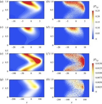
Two typical temporal concentration distributions  $\langle P\rangle _{O}(x,z,t)$ are plotted in figure 6. We see qualitatively different temporal evolutions between the two cases. In the case with weak overall shear (
 $\textit {Pe}_f=1$), a layer of high concentration quickly forms at the upper boundary, which is the trivial gravitactic focusing phenomenon (Bearon et al. Reference Bearon, Hazel and Thorn2011). In contrast, in the case with strong overall shear (
 $\textit {Pe}_f=10$), although micro-swimmers diffuse more quickly in the streamwise
 $x$-direction, a layer of high concentration forms just above the centreline and persists for a considerable time. In addition, in such a case, the concentration difference between the bottom area and the upper area is not as obvious as that in the weak overall shear case, due to the equally strong resistance to upward migration at the bottom high shear region.
Transient two-dimensional concentration distributions  $\langle P \rangle _{O}(x,z,t)$ of a vertically uniform line-source release of non-settling gyrotactic micro-swimmers in the plane Poiseuille flow: (a), (c), (e), (g) concentration distributions obtained with the Edgeworth series expansion; (b), (d), (f), (h) concentration distributions directly obtained with the IBM simulations (see Appendix A); (a)–(d)
 $\textit {Pe}_f=1$ and (e)–(h)
 $\textit {Pe}_f=10$; (a), (b), (e), ( f)
 $t=5$; (c), (d), (g), (h)
 $t=10$. Common parameters:
 $\textit {Pe}_s=0.1$,
 $\lambda =5$,
 $D_t=0.01$. Note that the aspect ratio and maximum concentration of the colour-bar are modified in each panel to enhance visualisation.

As the plane Poiseuille flow has a linearly varying rate of shear, which is similar to the flow configuration of the experiment by Durham et al. (Reference Durham, Kessler and Stocker2009), we can make a rough estimation of the relevant parameter in the experiment: we get  $\textit {Pe}_s\sim {O}(10^{-1})$,
 $\textit {Pe}_f \sim {O}(10)$ and
 $\lambda \sim {O}(1)$ by converting the documented data in Durham et al. (Reference Durham, Kessler and Stocker2009) according to the definitions in (2.10). This parameter space is consistent with our results when the transient thin layers are observed. The case with a larger
 $\textit {Pe}_s$ but still small enough compared with
 $\textit {Pe}_f$ has been qualitatively discussed by Durham et al. (Reference Durham, Kessler and Stocker2009) and has also been shown in our results that a more intensive thin layer will appear (see e.g. figure 3l).
3.1.2. Settling micro-swimmers
Whether thin phytoplankton layers are persistent or transient is an open and crucial question. Their time scales can range from several weeks in real ocean to several minutes such as in the experiment by Durham et al. (Reference Durham, Kessler and Stocker2009). However, up to now, we do not see any steady thin layer in our analysis: all transient thin layers dissipate at the asymptotic long-time due to diffusion and positive up-swimming speed. This assertion has also been confirmed by former results obtained with the two-step GTD method and the IBM (Bearon et al. Reference Bearon, Hazel and Thorn2011; Ghorai Reference Ghorai2016), under a similar initial condition setup (finite micro-swimmer numbers), as well as by dynamic system analysis for a laminar Kolmogorov flow (Santamaria et al. Reference Santamaria, De Lillo, Cencini and Boffetta2014). It can be also supported by considering the effect of Jeffery's torque on a sphere, which merely rotates the orientation of a micro-swimmer without a preferable angle. Therefore, the gyrotaxis, although maybe weak compared with the tumbling effect of the shear, can still contribute to a small upward migration given time long enough and, finally, leads to the disappearance of the transient thin layers. We note that, although a steady thin layer was not found in the previous discussion, we can see that the shear can extend the time necessary to reach the steady state, which implies that micro-swimmers can have more time to stay in the sub-surface area. As noted in § 1, micro-organisms can display convergent swimming behaviour to the sub-surface nutricline to get nourishment and reproduce. In the current case, shear also enables the micro-swimmers to stay temporarily in the bulk, serving as a possible interpretation for the thin phytoplankton layer if cells’ reproduction is considered.
Micro-swimmers such as marine micro-organisms are typically negatively buoyant. For example, the settling speed of C. nivalis is about  $10\,\%$ of the swimming speed (Hwang & Pedley Reference Hwang and Pedley2014). Settling speed has been shown to be critical to the stability of the gyrotactic micro-organisms suspension (Plesset & Winet Reference Plesset and Winet1974; Childress, Levandowsky & Spiegel Reference Childress, Levandowsky and Spiegel1975; Pedley, Hill & Kessler Reference Pedley, Hill and Kessler1988; Hwang & Pedley Reference Hwang and Pedley2014; Bees Reference Bees2020) and serves as a possible explanation (Maretvadakethope, Keaveny & Hwang Reference Maretvadakethope, Keaveny and Hwang2019) for the transient thin layer if one considers a higher concentration suspension and the resultant instability. Using the identical two-step GTD method of Bearon et al. (Reference Bearon, Hazel and Thorn2011), Ghorai (Reference Ghorai2016) found that steady thin layers do appear with a small settling speed (
 $0.1\textit {Pe}_s$). Sub-surface thin layer caused by sedimentation is also found by Maretvadakethope et al. (Reference Maretvadakethope, Keaveny and Hwang2019), using the more primitive P–K model.
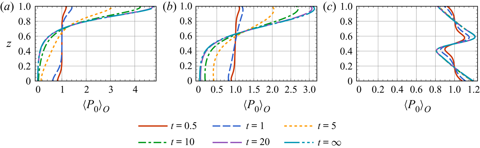
Now, using the method developed in § 2, we investigate whether sedimentation could maintain the thin layer in the plane Poiseuille flow. Three evolution processes of vertical distribution with  $\textit {Pe}_d=0.1\textit {Pe}_s$ are plotted in figure 7. Interestingly, different from the transient thin layer observed in the non-settling cases, we see a steady thin layer with the inclusion of a non-zero settling speed in the case with strong overall shear (figure 7(c),
 $\textit {Pe}_f=10$). This is understood by the fact that the settling flux counteracts the small and positive upward swimming flux indicated in figure 5(c). The gravitactic focusing mechanism is greatly inhibited by the combined effect of high shear at the boundary and the sedimentation, as can be seen from the big concentration drop at the upper surface compared with figure 3( f). In addition, the concentration at the bottom also shows a different evolution process compared with the non-settling case: without sedimentation, the concentration gets smaller at the bottom, whereas the concentration at the bottom increases monotonically due to the combined effect of strong shear and sedimentation in the case with sedimentation.
Transient vertical distributions  $\langle P_0 \rangle _{O}$ of a vertically uniform line-source release of settling gyrotactic micro-swimmers in the plane Poiseuille flow: (a)
 $\textit {Pe}_f=0.1$; (b)
 $\textit {Pe}_f=1$; (c)
 $\textit {Pe}_f=10$. Common parameters:
 $\textit {Pe}_s=0.1$,
 $\textit {Pe}_d=0.01$,
 $\lambda =5$,
 $D_t=0.01$.

3.2. Tanh flow
The tanh flow is conceptualised by Durham et al. (Reference Durham, Kessler and Stocker2009) to represent typical regions where thin layers are found. The velocity profile of the tanh flow is
 \begin{equation} U(z)=\coth\left(\frac{1}{2\delta}\right)\tanh \left(\frac{z-0.5}{\delta}\right). \end{equation}
Consistent with Bearon et al. (Reference Bearon, Hazel and Thorn2011), we use  $\delta = 0.05$ in our analysis. Different from the plane Poiseuille flow, the tanh flow profile is antisymmetric with respect to
 $z=0.5$. In addition, it provides a high shear layer of thickness
 $\delta$ around
 $z=0.5$. Note that although the tanh flow does not satisfy the Navier–Stokes equation without artificial body force (Bearon et al. Reference Bearon, Hazel and Thorn2011), it can be seen as a benchmark to study gyrotactic trapping (Bearon et al. Reference Bearon, Hazel and Thorn2011; Ishikawa Reference Ishikawa2012; Ghorai Reference Ghorai2016).
3.2.1. Non-settling gyrotactic micro-swimmer
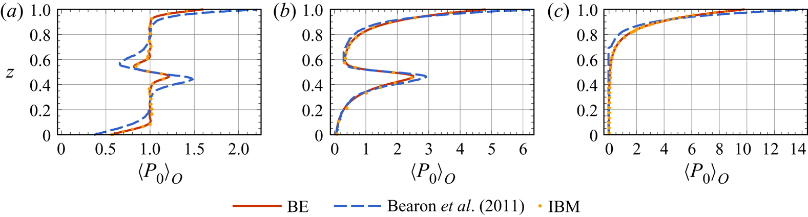
As noted previously, the local equilibrium hypothesis is not accurate enough for flows with rapidly changing shear. The tanh flow, however, is actually such a flow. In figure 8 we show the comparison of our results and the results of Bearon et al. (Reference Bearon, Hazel and Thorn2011), which are calculated with the two-step GTD method. Also plotted are the IBM results: for the transient vertical distributions at  $t=1$ and
 $10$, there is no difference between our IBM results and those of Bearon et al. (Reference Bearon, Hazel and Thorn2011); because there is no available steady-state vertical distribution obtained with IBM simulation in Bearon et al. (Reference Bearon, Hazel and Thorn2011), the plotted IBM steady-state vertical distribution is from our simulation at
 $t=500$ with convergence attained by comparing with
 $t=600$. We see that our results based on the biorthogonal expansion are in good agreement with the IBM results, while discrepancies between the two-step GTD method and IBM arise. At
 $t=1$, as shown in figure 8(a), two-step GTD method overestimates the concentration depletion at the bottom and at the upper boundary of the shear layer (
 $z\approx 0.6$), and the concentration increment at the top and at the lower boundary of the shear layer (
 $z\approx 0.4$). The inaccurate prediction of two-step GTD method at the early stage, i.e.
 $t=1$ is mainly due to the neglect of initial condition in the orientational space: micro-swimmers have uniform orientational distribution initially, while this cannot be considered by the two-step GTD method. The predictions at the top also suffer this neglect and one more due to the neglect of influential boundary effect, as depicted in figure 8(b,c).
Comparison of vertical distributions  $\langle P_0 \rangle _{O}$ of a vertically uniform line-source release of non-settling gyrotactic micro-swimmers between the current model, Bearon et al. (Reference Bearon, Hazel and Thorn2011) and IBM. ‘BE’ stands for result obtained with biorthogonal expansion: (a)
 $t=1$; (b)
 $t=10$; (c)
 $t=\infty$. Parameters:
 $\textit {Pe}_f=0.5$,
 $\textit {Pe}_s=0.1$,
 $\textit {Pe}_d=0$,
 $\lambda =1$,
 $D_t=0$.

We now discuss the variations of the transient thin layer. The evolution processes of vertical concentration distribution  $\langle P_0 \rangle _{O}$ of a line-source release of non-settling micro-swimmers in the tanh flow are plotted in figure 9, where we see obvious transient thin layers in cases where the micro-swimmers are highly active (
 $\textit {Pe}_s =1$). As discussed in § 3.1.1, large
 $\textit {Pe}_s$ causes a strong upward migration flux gradient to the high shear region at the centre, thus the trapping is more intensive. Instead, in cases where
 $\textit {Pe}_s$ is small, as depicted in figure 9(a) and 9(b), there are micro-swimmers transiently trapping in the high shear region, but the thickness is broadened and maximum concentration is weakened due to a weak upward flux gradient and a relatively strong diffusion. It is seen in figures 8 and 9 that transient thin layer can be observed as long as
 $\textit {Pe}_f \geqslant 1$. As the non-dimensional maximum local shear rate (located at
 $z=0.5$) in the tanh flow equals
 $20$, we can infer that the dimensional maximum local shear rate
 $\approx 0.01\,\mathrm {s}^{-1}$, if
 $D_r^{\ast }=0.01\,\mathrm {s}^{-1}$ and
 $H^{\ast } = 10\,\mathrm {m}$ are chosen according to Durham et al. (Reference Durham, Kessler and Stocker2009). This range of shear rate is comparable to typical values observed in thin layers (Dekshenieks et al. Reference Dekshenieks, Donaghay, Sullivan, Rines, Osborn and Twardowski2001; Ryan et al. Reference Ryan, McManus, Paduan and Chavez2008; Durham & Stocker Reference Durham and Stocker2012). Lastly, as depicted in figure 9, the steady states of all cases do not contain thin layers which can be observed transiently. Note that cases with small
 $\lambda$ are also examined but the thin layer still does not persist, these cases are not shown here.
Transient vertical distributions  $\langle P_0 \rangle _{O}$ of a vertically uniform line-source release of non-settling gyrotactic micro-swimmers in the tanh flow: (a)
 $\textit {Pe}_f=1$,
 $\textit {Pe}_s=0.1$; (b)
 $\textit {Pe}_f=10$,
 $\textit {Pe}_s=0.1$; (c)
 $\textit {Pe}_f=1$,
 $\textit {Pe}_s=1$; (d)
 $\textit {Pe}_f=10$,
 $\textit {Pe}_s=1$. Common parameters:
 $\lambda =5$,
 $D_t=0.01$.

3.2.2. Settling gyrotactic micro-swimmer
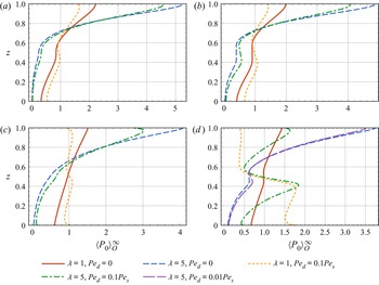
The steady vertical distributions  $\langle P_0\rangle _{O}^{\infty }$ of micro-swimmers with and without sedimentation in the tanh flow are plotted in figure 10. We see that obvious steady thin layer do exist in one case, namely the case with
 $\textit {Pe}_s=1$,
 $\textit {Pe}_f=10$,
 $\textit {Pe}_d=0.1$ and
 $\lambda =5$ in figure 10(d), this is also the case where we find the most obvious transient thin layer in figure 9(d). In cases where the overall shear is not strong enough (see e.g. figure 10a and 10c) or the sedimentation is weak (figure 10b),
 $\textit {Pe}_d=0.01$), the micro-swimmers still show gravitactic focusing at the upper surface. For the cases with weak overall shear, it is understood by a negligible gyrotactic trapping mechanism, whereas the cases with weak sedimentation are attributed to a relatively strong up-swimming velocity dominating over the settling speed. This is also seen in figure 10(d) by comparing the vertical distributions of micro-swimmers with the same swimming speed (
 $\textit {Pe}_s=1$) and gyrotactic bias (
 $\lambda =5$) but different settling speeds (
 $\textit {Pe}_d=0.1$ and
 $0.01$). Only when both the flow and sedimentation are strong do the steady thin layer exist. Note that the thin layer formed by the micro-swimmers with more intensive gyrotaxis (
 $\lambda =5$) is more like a typical thin layer, whereas the less gyrotactic one (
 $\lambda =1$) is not due to the high concentration also at the bottom.
Steady state of the vertical distributions  $\langle P_0 \rangle _{O}^{\infty }$ of spherical gyrotactic micro-swimmers in the tanh flows: (a)
 $\textit {Pe}_f=1, \textit {Pe}_s=0.1$; (b)
 $\textit {Pe}_f=10, \textit {Pe}_s=0.1$; (c)
 $\textit {Pe}_f=1, \textit {Pe}_s=1$; (d)
 $\textit {Pe}_f=10, \textit {Pe}_s=1$. Common parameters:
 $D_t=0.01$.

4. Generalisation to unconstrained rotation
We now generalise our analysis to situation of unconstrained rotation. This generalisation paves the way to analyse cases with general three-dimensional unidirectional flows. We make a comparison between the constrained rotation cases (i.e. two-dimensional micro-swimmers with one rotational degree of freedom, denoted by  $1$-RD) and the unconstrained rotation cases (with two rotational degrees of freedom, denoted by
 $2$-RD). In addition, a direct comparison between the results of the biorthogonal expansion method and the results of two-step GTD method in unconstrained rotation cases are also discussed.
4.1. Comparison with constrained rotation
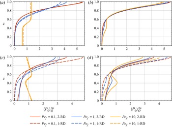
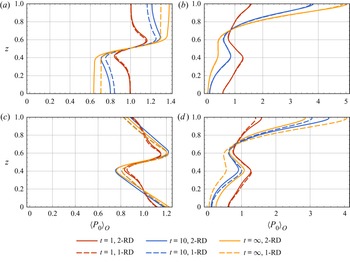
The comparison of the steady vertical distributions  $\langle P_0 \rangle _{O}^{\infty }$ between the
 $1$-RD and
 $2$-RD cases is plotted in figure 11, and the comparison of the transient vertical distributions
 $\langle P_0 \rangle _{O}$ is plotted in figure 12. We see that in cases without sedimentation, a stronger overall shear (
 $\textit {Pe}_f=1,10$) leads to observable differences of both the steady and the transient concentration at the boundaries in the Poiseuille flow (figures 11a and 12a), whereas the concentration slightly varies in the tanh flow (figures 11b and 12b). Compared with the
 $1$-RD cases, the gravitactic focusing at the upper boundary is enhanced in the
 $2$-RD cases. This reflects that the new rotational degree of freedom relieves the effect of the flow shear interrupting up-swimming. However, the new rotational degree of freedom plays a more complex role in the cases with sedimentation. As shown in figures 11(c) and 11(d) and 12(c) and 12(d), although the
 $2$-RD and
 $1$-RD cases have almost the same vertical distribution in the Poiseuille flow with
 $\textit {Pe}_f=10$, gravitactic focusing at the upper boundary is largely weakened by the new rotational degree of freedom in most cases. For example, figure 11(d) shows that in the tanh flow with
 $\textit {Pe}_f=10$, the concentration at
 $z=1$ drops from
 $4.8$ in the
 $1$-RD case to
 $3.6$ in the
 $2$-RD case. Moreover, in the
 $2$-RD cases, the steady gyrotactically trapped layer occurred in the tanh flow is largely enhanced with a nearly doubled maximum concentration (figure 11(d),
 $\textit {Pe}_f=10$).
Comparison of the steady vertical distributions  $\langle P_0 \rangle _{O} ^{\infty }$ of spherical gyrotactic micro-swimmers with one rotational degree of freedom (denoted by ‘
 $1$-RD’) and two rotational degrees of freedom (denoted by ‘
 $2$-RD’): (a) non-settling gyrotactic micro-swimmers in the Poiseuille flow; (b) non-settling gyrotactic micro-swimmers in the tanh flow; (c) settling gyrotactic micro-swimmers with
 $\textit {Pe}_d=0.01$ in the Poiseuille flow; (d) settling gyrotactic micro-swimmers with
 $\textit {Pe}_d=0.01$ in the tanh flow. Common parameters:
 $\textit {Pe}_s=0.1, D_t=0.01$,
 $\lambda =5$,
 $\alpha _0=0$.

Comparison of the transient vertical distributions  $\langle P_0 \rangle _{O}$ of spherical gyrotactic micro-swimmers with one rotational degree of freedom (denoted by ‘
 $1$-RD’) and two rotational degrees of freedom (denoted by ‘
 $2$-RD’): (a) non-settling gyrotactic micro-swimmers in the Poiseuille flow; (b) non-settling gyrotactic micro-swimmers in the tanh flow; (c) settling micro-swimmers with
 $\textit {Pe}_d=0.01$ in the Poiseuille flow; (d) settling micro-swimmers with
 $\textit {Pe}_d=0.01$ in the tanh flow. Both
 $1$-RD and
 $2$-RD cases are calculated with vertical uniform line-source releases, with the initial orientations of the micro-swimmers uniformly distributed in the
 $x$–
 $z$ plane. Common parameters:
 $\textit {Pe}_s=0.1$,
 $\textit {Pe}_f=10$,
 $D_t=0.01$,
 $\lambda =5$,
 $\alpha _0=0$.

4.2. Comparison with two-step GTD method
Now we use  $C(z,t)$ to denote the vertical concentration of the two-step GTD method. The governing equation used in the two-step GTD method is
 \begin{equation} \frac{\partial{C}}{\partial t} ={-}\textit{Pe}_s \langle p_z \rangle_{{G}} \frac{\partial{C}}{\partial z} - \textit{Pe}_s C \frac{\partial \langle p_z\rangle_{{G}}}{\partial z} + \textit{Pe}_d \frac{\partial C}{\partial z} +\frac{\partial}{\partial z}\left(D_{zz} \frac{\partial C}{\partial z}\right) + D_t \frac{\partial^2 C}{\partial z^2}, \end{equation}
where  $\langle p_z \rangle _{{G}}$ is the mean up-swimming orientation component and
 $D_{zz}$ is the vertical dispersivity. Importantly, neglecting the sedimentary flux gradient
 $\textit {Pe}_d\partial C/\partial z$ and Brownian translational diffusive flux gradient
 $D_t \partial ^2 C /\partial z^2$ and then comparing (4.1) with (3.2), one finds that
 $-\partial J_z/\partial z$ in (3.2) corresponds to the sum of both the swimming flux gradient (first two terms on the right-hand side of (4.1)) and the dispersive flux gradient (fourth term on the right-hand side of (4.1)). However, (3.2), which is directly from the Smoluchowski equation, does not contain such a dispersive flux gradient. Therefore, if one knows exactly the accurate instantaneous mean up-swimming orientation component
 $\langle p_z \rangle _{{O}}$, there is probably no need to add a dispersive flux gradient for the transport. Without the a priori information of the exact
 $P$ and, thus,
 $\langle p_z \rangle _{{O}}$, the two-step GTD method uses
 $\langle p_z \rangle _{{G}}$ that only depends on the local shear instead and adds a dispersive flux based on the phenomenological diffusivity
 $D_{zz}$. Specifically,
 $\langle p_z \rangle _{{G}}$ and
 $D_{zz}$ are calculated by assuming unbounded flow with homogeneous shear in the asymptotic limit (
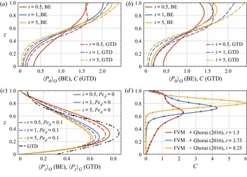
 $t \gg 1$). Note that, Fung, Bearon & Hwang (Reference Fung, Bearon and Hwang2022) recently transformed the Smoluchowski equation to an exact drift–diffusion equation in the positional space. Their approach differs from the two-step GTD method in predicting the drift and diffusion coefficients. Assuming orientation–position separation and thus using local flow information only, their new model can be closed using a multiple-time-scale technique and the results are in good agreement with full numerical solution of the Smoluchowski equation in some parameter ranges.
In the comparison here, we choose micro-swimmers with a strong swimming ability  $\textit {Pe}_s=1$ to strengthen the difference between the results of biorthogonal expansion and two-step GTD method. Plotted in figure 13 is a direct comparison of transient vertical distributions (
 $\langle P_0\rangle _{{O}}$ for BE and
 $C$ for two-step GTD) and mean up-swimming orientation component (
 $\langle p_z\rangle _{{O}}$ for BE and
 $\langle p_z\rangle _{{G}}$ for two-step GTD) of a vertically uniform line-source release of micro-swimmers between the current model and two-step GTD method in unconstrained rotation cases. The results of two-step GTD method are calculated with a finite volume method (FVM) based on the given mean up-swimming orientation component
 $\langle p_z \rangle _{{G}}$ and vertical diffusivity component
 $D_{zz}$ in Ghorai (Reference Ghorai2016). In the two-step GTD method,
 $\langle p_z \rangle _{{G}}$ only depends on variables that influence the local rotation (Bearon et al. Reference Bearon, Hazel and Thorn2011; Ghorai Reference Ghorai2016), i.e.
 $\lambda$,
 $\alpha _0$,
 $\textit {Pe}_f$ and
 $U$. These variables are kept the same with Ghorai (Reference Ghorai2016) in both our biorthogonal expansion and FVM calculation. Here
 $D_{zz}/\textit {Pe}_s^2$ also only depends on variables that influence the local rotation (Manela & Frankel Reference Manela and Frankel2003; Bearon et al. Reference Bearon, Hazel and Thorn2011; Ghorai Reference Ghorai2016; Fung et al. Reference Fung, Bearon and Hwang2020), thus
 $D_{zz}$ in cases with a different
 $\textit {Pe}_s$ can be easily obtained. The FVM method is validated against published data in Ghorai (Reference Ghorai2016), as shown in figure 13(d).
Comparison of (a), (b) transient vertical distributions and (c) the mean up-swimming orientation components of a vertically uniform line-source release of micro-swimmers between the biorthogonal expansion method and two-step GTD method: (a)  $\textit {Pe}_d=0$ and (b)
 $\textit {Pe}_d=0.1$. Micro-swimmers with a strong swimming ability
 $\textit {Pe}_s=1$ are chosen to strengthen the difference. The two-step GTD results are calculated with a FVM method based on the given mean up-swimming orientation component
 $\langle p_z \rangle _{{G}}$ and vertical diffusivity
 $D_{zz}$ component in Ghorai (Reference Ghorai2016). The validation of FVM against the published data in Ghorai (Reference Ghorai2016) with
 $\textit {Pe}_s=0.252$,
 $\textit {Pe}_d=0.1\textit {Pe}_s$ is given in (d). In all cases, the velocity profile of the background parabolic flow is
 $U=3z^2-2z$,
 $\textit {Pe}_f=7$,
 $\lambda =6.667$. Here
 $D_t=0.1$ in all cases except for (d), where
 $D_t=0$ for consistency with Ghorai (Reference Ghorai2016).

For the comparison between the current model and the two-step GTD method plotted in figure 13(a) and 13(b), we see that the results show obvious differences due to highly active micro-swimmers sampling strongly varying shear. In addition, the accurate mean up-swimming orientation component  $\langle p_z\rangle _{{O}}$ is time-dependent and sedimentation-dependent, which is not reflected by
 $\langle p_z\rangle _{{G}}$. Furthermore, the difference of mean up-swimming orientation component at the boundaries between the models signifies the failure of two-step GTD method to represent the boundary conditions in the phase space
 $(z,\theta )$ (Bearon et al. Reference Bearon, Hazel and Thorn2011).
5. Concluding remarks
The thin phytoplankton layer has been identified as an important phenomenon occurring in coastal regions and stratified lakes. In this paper, using a continuum approach based on the Smoluchowski equation, we have studied the gyrotactic trapping mechanism first suggested by Durham et al. (Reference Durham, Kessler and Stocker2009). There have been several attempts to simplify the high-dimensional Smoluchowski equation to a drift–diffusion equation in the positional space, such as the primitive P–K model (Pedley & Kessler Reference Pedley and Kessler1990; Zeng & Pedley Reference Zeng and Pedley2018), better GTD model (Hill & Bees Reference Hill and Bees2002; Manela & Frankel Reference Manela and Frankel2003; Bearon et al. Reference Bearon, Hazel and Thorn2011), and more complex model (Fung et al. Reference Fung, Bearon and Hwang2022). However, the local equilibrium hypothesis and the neglect of boundary conditions in phase space are the major restrictions when we try to apply these models to cases with strongly varying shear and non-negligible boundary effect. Generally speaking, although gyrotactic trapping in oceans often occurs in regions where the shear varies strongly, the associated length scale is still much larger than the swimming length scale of the micro-organisms; in the meantime, the water column is deep enough to be with negligible boundary effect; thus, these models may be acceptable. However, in laboratory studies and engineering practices, the applicability of these models needs further consideration as the associated length scale of shear variation can be much smaller and the boundary effect can be influential.
In this paper, extending the method of Jiang & Chen (Reference Jiang and Chen2021), we have given a more complete picture of gyrotactic trapping. The equations governing the local moments have been solved by making an eigenfunction expansion and applying a biorthogonal expansion to the eigenfunctions. A constant settling speed, which was not included in Jiang & Chen (Reference Jiang and Chen2021), is assumed in some cases, and the associated boundary conditions are derived by analysing the fluxes balance. We use the reflective boundary conditions to derive the corresponding basis functions, thus all information of the boundary conditions in the phase space is retained. In contrast, two-step GTD method only involves boundary conditions in the positional space, such as zero-flux and free-stream boundary conditions. Our results are in good agreement with the IBM simulations due to no approximation made to the fundamental Smoluchowski equation.
As a practical configuration, the transport of gyrotactic micro-swimmers in the plane Poiseuille flows was first investigated. Qualitatively consistent with previous studies, transient layers of high concentration are found in cases where the overall shear is strong, indicating the hindrance of shear rotation to vertical migration of micro-organisms, exactly characteristic of gyrotactic trapping. Although steady thin layers do not appear without sedimentation, the duration of the transient thin layers can be extended largely by the flow intensity, implying the strong disruption of shear on the vertical migration of micro-swimmers. The residence of micro-swimmers in the subsurface area may be a favourable condition for their reproduction at nutriclines. Furthermore, the time-dependent characteristic of the mean up-swimming orientation component  $\langle p_z\rangle _{{O}}$ shows the inaccurate steady average swimming orientation assumed in the two-step GTD method. We next consider a constant settling speed for micro-swimmers to reflect the fact that most phytoplankton is denser than the ambient fluid. Steady thin layers are observed after including a settling speed, which is consistent with former study.
We have also investigated the transport of gyrotactic micro-swimmers in the tanh flow, which contains a high shear region in the middle and has previously been studied intensively. Our results have been compared directly with the results of former two-step GTD as well as results of IBM. Our results are in good agreement whereas the two-step GTD method deviates to some extent. We find that transient thin layers can be observed as long as the flow is strong enough to tumble the micro-swimmers rapidly in the high shear region. However, the steady thin layer is also not observed until the inclusion of a constant settling speed.
Finally, we have discussed the situation of unconstrained rotation. For the comparison between unconstrained rotation and constrained rotation, although the results are qualitatively similar, we see noticeable differences, especially with a strong overall shear. Care must be taken when investigating three-dimensional micro-swimmers. For the comparison between the current method and two-step GTD method, we see obvious differences highlighting the inaccuracy of the two-step GTD method again.
This work bridges the gap between the continuum approach and IBM. However, we do not expect that we are very close to the real situation where the thin phytoplankton layers occur, as the flow and micro-swimmer model considered are relatively simple. First, the micro-swimmer–boundary interaction is not our major point and we have mainly considered the reflective boundary conditions, which are a simple and idealised micro-swimmer–boundary steric interaction. Sperm (Rothschild Reference Rothschild1963) and E. coli (Berke et al. Reference Berke, Turner, Berg and Lauga2008) have been reported to have a strong tendency to adhere to walls. The Robin boundary conditions are a set of boundary conditions that can qualitatively account for this phenomenon. Although we show in Appendix B that in some cases gyrotactic trapping in the bulk is not very sensitive to the choice of boundary conditions, it is still an open question that how to describe the behaviours of micro-swimmers on a continuum scale, as the behaviours vary from species to species and from environment to environment (Lauga et al. Reference Lauga, DiLuzio, Whitesides and Stone2006; Li, Tam & Tang Reference Li, Tam and Tang2008; Li & Tang Reference Li and Tang2009; Kantsler et al. Reference Kantsler, Dunkel, Polin and Goldstein2013). The reflective boundary conditions are the simplest and may fail to describe the complex boundary behaviours. Researches investigating the complex behaviours of micro-swimmers near boundaries are hot-spots recently (Li et al. Reference Li, Tam and Tang2008; Kantsler et al. Reference Kantsler, Dunkel, Polin and Goldstein2013; Bianchi et al. Reference Bianchi, Saglimbeni, Frangipane, Dell'Arciprete and Leonardo2019), however, less is developed for the continuum description of the behaviours and further works regarding this are welcome. In addition, assuming the micro-swimmers to be point-size is also not accurate for very narrow channel (Ezhilan & Saintillan Reference Ezhilan and Saintillan2015; Chen & Thiffeault Reference Chen and Thiffeault2021).
Second, the flows we use are steady, laminar and unidirectional. In such a configuration, the one-step GTD method and the biorthogonal expansion method are shown to be superior to other methods based on the local equilibrium hypothesis. However, the flows in real water environments such as oceans are mostly turbulent and multi-directional, where the biorthogonal expansion method is not applicable. The P–K model and two-step GTD method are probably able to deal with such situations. Improvements on these more general methods are therefore highly desired, such as a recent work by Fung et al. (Reference Fung, Bearon and Hwang2022). Moreover, we assumed the flow to be two-dimensional. However, the approach we used can be applied to three-dimensional flows as long as the flow is unidirectional and bounded by a cross-section.
Apart from the flow, the settling micro-swimmer considered in this paper is spherical. Elongated settling micro-swimmers can exhibit more complex dynamics due to an orientation-dependent settling speed (Ruiz, Macías & Peters Reference Ruiz, Macías and Peters2004; Ardekani et al. Reference Ardekani, Sardina, Brandt, Karp-Boss, Bearon and Variano2017; Clifton et al. Reference Clifton, Bearon and Bees2018) and possible non-negligible inertial effects (Dabade, Marath & Subramanian Reference Dabade, Marath and Subramanian2015; Lopez & Guazzelli Reference Lopez and Guazzelli2017; Sheikh et al. Reference Sheikh, Gustavsson, Lopez, Lévêque, Mehlig, Pumir and Naso2020; Qiu et al. Reference Qiu, Cui, Climent and Zhao2021). Another important aspect not involved in this study is the effect of micro-swimmers’ negative buoyancy on the flow. We have restricted our attention to a very dilute suspension and neglected the possible instability. Nonetheless, a recent work based on the P–K model by Maretvadakethope et al. (Reference Maretvadakethope, Keaveny and Hwang2019) revealed that the gyrotactically trapped layer can be unstable at a much more dilute concentration ( $10^4\ \mathrm {cells}\ \mathrm {cm}^{-3}$) than the typical value at which bioconvection occurs (
 $10^6\ \mathrm {cells}\ \mathrm {cm}^{-3}$ (Bees Reference Bees2020)), due to the coupling of sedimentation-induced flow and the background flow. As the P–K model is not satisfactory at high shear rate (Croze et al. Reference Croze, Bearon and Bees2017; Fung et al. Reference Fung, Bearon and Hwang2020), it is necessary to investigate the stability of the gyrotactically trapped layer with more precise models or directly from the Smoluchowski equation. In addition, cell–cell hydrodynamic interactions should be considered in a relatively dense suspension. For example, although Ishikawa (Reference Ishikawa2012) used the same drift–diffusion equation in the positional space, the drift and diffusion origin from non-Brownian cells’ near-field hydrodynamic interactions, which are volume-fraction-dependent.
Funding
This work is supported by the National Natural Science Foundation of China (Grant Nos 52079001, 51879002 and 52109093). W.J. acknowledges the support of China Postdoctoral Science Foundation (Grant No. 2021M701906) and the Shuimu Tsinghua Scholar Program.
Declaration of interests
The authors report no conflict of interest.
Appendix A. IBM
Here we introduce the IBM of two-dimensional micro-swimmers. The stochastic differential equations governing the translational and orientational motions of a gyrotactic micro-swimmer (Jiang & Chen Reference Jiang and Chen2021) are discretised with a simple forward Euler scheme:
 $$\begin{gather} \Delta x=\textit{Pe}_f U \Delta t +\textit{Pe}_s \cos \theta \Delta t +\Delta x^B, \end{gather}$$
 $$\begin{gather}\Delta z=\textit{Pe}_s \sin \theta \Delta t -\textit{Pe}_d \Delta t + \Delta z^B, \end{gather}$$
 $$\begin{gather}\Delta \theta=\left(-\frac{1}{2}\textit{Pe}_f \frac{\partial U}{\partial z}+\frac{1}{2}\alpha_0 \textit{Pe}_f \frac{\partial U}{\partial z}\cos2\theta+\lambda \cos\theta\right)\Delta t + \Delta \theta^B, \end{gather}$$
where  $\Delta t$ is the time step, and
 $\Delta x^B$ and
 $\Delta z^B$ are noises characterising translational diffusion and are sampled from two independent normal distributions
 $N(0,2D_t \Delta t)$. Similarly, sampled from a normal distribution
 $N(0,2 \Delta t)$,
 $\Delta \theta ^B$ is the noise characterising the rotational diffusion. Using
 $(x_n,z_n,\theta _n)$ to denote the
 $n$th step position of a micro-swimmer, the reflective boundary conditions implemented in IBM are
 \begin{equation} \left.\begin{array}{lll@{}} z_n \rightarrow 2 - z_n, & \theta_n \rightarrow -\theta_n, & \mathrm{if} \ z_n >1,\\ z_n \rightarrow - z_n, & \theta_n \rightarrow -\theta_n, & \mathrm{if} \ z_n <0, \end{array}\right\} \end{equation}
where ‘ $\rightarrow$’ denotes assignment. We use
 $10^5$ micro-swimmers for each realisation, consistent with Bearon et al. (Reference Bearon, Hazel and Thorn2011) and close to Peng & Brady (Reference Peng and Brady2020). A time step
 $\Delta t=10^{-4}$ is used and the convergence is tested by comparing the moments obtained with
 $\Delta t=10^{-5}$.
The vertical distribution of IBM simulations is obtained by counting the numbers of micro-swimmers in 100 equal intervals in the vertical direction. As some vertical distributions  $\langle P_0 \rangle _{{O}}$ obtained by the biorthogonal expansion have been or will be validated against the IBM simulations (e.g. figures 8, 15 and 17), here we present the comparison of higher-order quantities, namely drift velocity
 $U_d$, dispersivity
 $D_T$ and skewness
 $\gamma _1$ defined as (Jiang & Chen Reference Jiang and Chen2021)
 $$\begin{gather} U_d(t) \triangleq \frac{\mathrm{d}M_1}{\mathrm{d}t}, \end{gather}$$
 $$\begin{gather}D_T(t) \triangleq \frac{1}{2}\frac{\mathrm{d} (M_2-M_1^2)}{\mathrm{d}t}, \end{gather}$$
 $$\begin{gather}\gamma_1(t) \triangleq \frac{M_3-3M_2M_1+2M_1^3}{(M_2-M_1^2)^{{3}/{2}}}, \end{gather}$$
where  $M_n (t)\triangleq \int _0^1 \int _0^{2{\rm \pi} } P_n(z,\theta,t) \, \mathrm {d}\theta \, \mathrm {d}z$ is the
 $n$th-order total moments. The moments of IBM simulations are calculated by
 \begin{equation} M_n = \frac{1}{10^5}\sum_{i=1}^{10^5} x_i^n, \end{equation}
where  $x_i$ is the horizontal coordinate of the micro-swimmer.
As shown in figure 14, the temporal drift velocity  $U_d$, dispersivity
 $D_T$ and skewness
 $\gamma _1$ between the two methods are in good agreement.
Comparison of temporal drift velocity  $U_d$, dispersivity
 $D_T$ and skewness
 $\gamma _1$ between the biorthogonal expansion and IBM simulations. Parameters:
 $\textit {Pe}_s=0.1$,
 $\textit {Pe}_d=0.01$,
 $\textit {Pe}_f=1$,
 $\lambda =5$,
 $D_t=0.01$. The background is a Poiseuille flow and the initial condition is a vertically uniform line-source release.

Appendix B. Alternative boundary conditions
As discussed by Ezhilan & Saintillan (Reference Ezhilan and Saintillan2015), the reflective boundary conditions are unable to reproduce the wall accumulation behaviour (Rothschild Reference Rothschild1963; Berke et al. Reference Berke, Turner, Berg and Lauga2008) of some micro-swimmers such as bacteria and sperm. Instead, the Robin boundary conditions, which were first used by Elgeti & Gompper (Reference Elgeti and Gompper2013), reproduce basic features such as wall accumulation and upstream swimming in confined environments (Elgeti & Gompper Reference Elgeti and Gompper2013; Ezhilan & Saintillan Reference Ezhilan and Saintillan2015; Jiang & Chen Reference Jiang and Chen2019; Peng & Brady Reference Peng and Brady2020; Chen & Thiffeault Reference Chen and Thiffeault2021). For two-dimensional micro-swimmers, one can easily write down the Robin boundary conditions by imposing the balance of p.d.f. between swimming flux, sedimentation flux and diffusion flux:
 \begin{equation} \textit{Pe}_s \sin \theta P -\textit{Pe}_d P-D_t \frac{\partial P}{\partial z} =0\quad \mbox{on} z=0,1, \quad \forall \, \theta \in [0,2{\rm \pi}),\end{equation}
which are actually setting the integrand in (2.16) to zero. When  $\textit {Pe}_d=0$, the boundary conditions above are widely used for non-settling micro-swimmers (Ezhilan & Saintillan Reference Ezhilan and Saintillan2015; Jiang & Chen Reference Jiang and Chen2019; Peng & Brady Reference Peng and Brady2020; Chen & Thiffeault Reference Chen and Thiffeault2021).
The Robin boundary conditions bring difficulty when solving the associated eigenvalue problem because of the dependence of  $P(x,z,\theta,t)$ on both
 $\theta$ and
 $z$. To avoid such complexity, we follow Jiang & Chen (Reference Jiang and Chen2019) to decompose
 $P(x,z,\theta,t)$ as follows:
 \begin{equation} P(x,z,\theta,t)=f_r(z) P_a(z,\theta) G^R(x,z,\theta,t) , \end{equation}
where
 \begin{equation} P_a(z,\theta)=\mathrm{exp}\left[\frac{\textit{Pe}_s \sin\theta}{D_t}\left(z-\frac{1}{2}\right)\right], \end{equation}
and  $f_r(z)$ is the transformation function defined in (2.22). The Robin boundary conditions for
 $P(x,z,\theta,t)$ are transformed to the boundary conditions for
 $G^R(x,z,\theta,t)$:
 \begin{equation} \frac{\partial G^R(x,z,\theta,t)}{\partial z}=0 \quad \mbox{on} \ z=0,1, \quad \forall \, \theta \in [0,2{\rm \pi}). \end{equation}
The basis functions for solving the moment equations under the Robin boundary conditions are
 \begin{equation} \left. \begin{array}{c@{}} \dfrac{1}{\sqrt{2{\rm \pi}}},\quad \dfrac{1}{\sqrt{\rm \pi}} \cos (n {\rm \pi}z), \quad \dfrac{1}{\sqrt{\rm \pi}}\cos (m \theta),\quad \dfrac{1}{\sqrt{\rm \pi}} \sin (m \theta), \\ \sqrt{\dfrac{2}{\rm \pi}}\cos (n {\rm \pi}z)\cos (m \theta) ,\quad \sqrt{\dfrac{2}{\rm \pi}} \cos (n {\rm \pi}z) \sin (m \theta). \end{array} \right \} \end{equation}
where  $m = 1, 2, \ldots$,
 $n = 1, 2, \ldots$.
The Robin boundary conditions are treated as a potential-free algorithm (Heyes & Melrose Reference Heyes and Melrose1993) in the IBM simulation (Peng & Brady Reference Peng and Brady2020). Physically, the potential-free algorithm demonstrates that when a micro-swimmer reaches the boundary, its orientation will not be altered by the boundary and will be still governed by the Jeffery equation (2.5) (Peng & Brady Reference Peng and Brady2020). The corresponding algorithm in the IBM simulation is
 \begin{equation} \left. \begin{array}{lll@{}} z_n \rightarrow 1, & \theta_n \rightarrow \theta_n, & \mathrm{if} \ z_n >1,\\ z_n \rightarrow 0, & \theta_n \rightarrow \theta_n, & \mathrm{if} \ z_n <0. \end{array} \right\} \end{equation}
We have noted in the main text that we mainly use the reflective boundary conditions. Generally speaking, the difference between the reflective boundary conditions and Robin boundary conditions can be weakened by a strong shear at the boundaries, due to the destructive of shear on the wall-normal polarisation structure under the Robin boundary conditions (Ezhilan & Saintillan Reference Ezhilan and Saintillan2015; Jiang & Chen Reference Jiang and Chen2019). Therefore, in the parameter region where thin layers are found, namely  $\textit {Pe}_f \sim {O}(10)$,
 $\textit {Pe}_s \sim {O}(0.1)$,
 $\textit {Pe}_d \sim {O}(0.1\textit {Pe}_s)$ and
 $\lambda \sim {O}(1)$, the steady vertical distributions
 $\langle P_0 \rangle _{{O}}^{\infty }$ under these two boundary conditions do not exhibit significant difference, as can be seen by comparing figure 15(b) with figure 7(c). In such a parameter space, the strong local shear at the boundaries is dominant, thus the difference between the reflective boundary conditions and Robin boundary conditions is small. It is inevitable that the vertical distribution can be sensitive to the boundary conditions in a relatively weak flow. For example, compared with figure 7(b), figure 15(a) shows that the wall accumulation effect underlying the Robin boundary conditions leads to an observable concentration increase at the upper surface. For the tanh flow, we can infer that the concentration increase at the upper boundary will be larger because the local shear rate is very weak.
Transient vertical distributions  $\langle P_0 \rangle _{{O}}$ under the Robin boundary conditions in a Poiseuille flow: (a)
 $\textit {Pe}_f=1$; (b)
 $\textit {Pe}_f=10$. IBM results at
 $t=100$ are plotted with dots. Common parameters:
 $\textit {Pe}_s=0.1$,
 $\textit {Pe}_d=0.01$,
 $\lambda =5$,
 $D_t=0.01$. The initial condition is a vertically uniform line-source release.

Actually, for cases with unbiased micro-swimmers in a still fluid, the Robin boundary conditions indicate a length scale of  $D_t/\textit {Pe}_s$ for the wall accumulation (Ezhilan & Saintillan Reference Ezhilan and Saintillan2015), and it can be also interpreted as an indicator for the length scale of the concentration boundary layer. We have chosen a relatively small
 $D_t=0.01$ to weaken the diffusion of the thin phytoplankton layer. However, this choice can be cumbersome in some cases under the Robin boundary conditions: when the local shear at the boundaries is weak (e.g. the Poiseuille flow with
 $\textit {Pe}_f=0.1$ and the tanh flow) and the swimming ability of the micro-swimmers is strong (e.g.
 $\textit {Pe}_s=1$), the concentration boundary layer becomes very thin and the concentration becomes very high, leading to a surge in the numbers of basis functions and the subsequent calculations (e.g. Bearon & Hazel Reference Bearon and Hazel2015). As we are concerned about a thin phytoplankton layer in the bulk, we do not pay much attention to the Robin boundary conditions with possible boundary accumulation effect.
It should be noted that other treatments mimicking micro-swimmers scattering at boundaries are also possible. For example, Kumar et al. (Reference Kumar, Thomson, Powers and Harris2021) used two alternative collision conditions for the IBM simulations of rods. One is assuming that the micro-swimmers are immediately aligned to the direction of the flow once the collision happens; another is assuming uniformly random collision angles. These treatments, along with the reflective and Robin boundary conditions, are idealised modelling of the micro-swimmer–boundary steric interactions. The real micro-swimmer–boundary interactions can be much more complicated (Drescher et al. Reference Drescher, Dunkel, Cisneros, Ganguly and Goldstein2011; Kantsler et al. Reference Kantsler, Dunkel, Polin and Goldstein2013; Bianchi, Saglimbeni & Di Leonardo Reference Bianchi, Saglimbeni and Di Leonardo2017; Bianchi et al. Reference Bianchi, Saglimbeni, Frangipane, Dell'Arciprete and Leonardo2019; Théry et al. Reference Théry, Wang, Dvoriashyna, Eloy, Elias and Lauga2021).
Appendix C. Effect of initial condition
It is evident that the initial condition will greatly affect the evolution process. For situation of two-dimensional micro-swimmers, we consider four different initial conditions, namely vertical uniform line-source releases with uniformly distributed orientations  $P_{ic}=1/(2{\rm \pi} )$, with orientation aligned upwardly
 $P_{ic}=\delta (\theta -{\rm \pi} /2)$ and with orientation aligned downwardly
 $P_{ic}=\delta (\theta -3{\rm \pi} /2)$, as well as a point-source release at the bottom with uniformly distributed orientations
 $P_{ic}=\delta (z)/(2{\rm \pi} )$. The vertical distributions at three early sample time ticks
 $t \in \{0.5,1,5\}$ are plotted in figure 16. We see that the three line-source releases do not coincide until
 $t=5$, demonstrating the unignorable influence of the initial orientational distribution. For the point-source release at the bottom, we see a much stronger trapped layer at
 $t=5$. Note that in the experiment by Durham et al. (Reference Durham, Kessler and Stocker2009), cells were also injected at the bottom.
Transient vertical distributions  $\langle P_0 \rangle _{O}$ of four different initial conditions in the tanh flows: (a)
 $t=0.5$; (b)
 $t=1$; (c)
 $t=5$. Common parameters:
 $\textit {Pe}_s=0.1$,
 $\textit {Pe}_d=0$,
 $\textit {Pe}_f=10$,
 $D_t=0.01$,
 $\lambda =5$.

Appendix D. Effect of micro-swimmer's elongation
In the main text, we have only considered the transient evolution of spherical micro-swimmers. However, micro-swimmers’ anisotropic geometry can be an influential factor in their dynamics: their orientations are affected not only by the vorticity-followed rotation but also by the shear-induced alignment effect due to strain rate. Shear-induced alignment effect causes elongated micro-swimmers to preferentially sample the streamlines (Pedley & Kessler Reference Pedley and Kessler1992). For example, in a pressure-driven microchannel flow, elongated micro-swimmers such as Bacillus subtilis exhibit trapping regime in the high-shear region (Rusconi et al. Reference Rusconi, Guasto and Stocker2014; Bearon & Hazel Reference Bearon and Hazel2015). It is also noteworthy that trapping regime in the low-shear region (near the channel centreline) can be also observed for micro-swimmers with an effective aspect ratio close to unity such as Heterosigma akashiwo (Barry et al. Reference Barry, Rusconi, Guasto and Stocker2015). This trapping regime results from the ‘back–forth swing’ across the channel centreline in strong flows (Rusconi et al. Reference Rusconi, Guasto and Stocker2014). Here, we choose rod-like (infinite aspect ratio) micro-swimmers, i.e.  $\alpha _0=1$ with three different flow Péclet numbers
 $\textit {Pe}_f \in \{0.1,1,10\}$ to investigate the effect of shape on the evolution of the vertical distribution of gyrotactic micro-swimmers with
 $\lambda =5$. As we have chosen a relatively large gyrotaxis intensity
 $\lambda$ (strong up-swimming tendency) and an infinite aspect ratio for the micro-swimmers, we can safely neglect the effects associated with low-shear trapping (Vennamneni et al. Reference Vennamneni, Nambiar and Subramanian2020, figure 14).
For situation of two-dimensional micro-swimmers, the transient vertical distributions of non-settling rod-like gyrotactic micro-swimmers in the plane Poiseuille flow obtained by both biorthogonal expansion and IBM simulation are plotted in figure 17. We see that in weak flow ( $\textit {Pe}_f=0.1$), the evolutions of the vertical distribution presented in figure 17(a) for rod-like micro-swimmers and figure 3(d) for spherical micro-swimmers are quantitatively similar, as expected by the negligible effect of the shear. However, when the flow gets strong (e.g.
 $\textit {Pe}_f=10$), there emerges an observable difference. As can be seen in figures 17(c) and 3( f), for the steady state, the maximum concentration at
 $z=1$ largely increases while the minimum concentration at
 $z=0$ largely diminishes in cases with the rod-like micro-swimmers. For the transient state, elongation enables micro-swimmers to escape the high-shear bottom boundary more quickly compared with spherical micro-swimmers. For example, when
 $t=5$ and
 $\textit {Pe}_f=10$, the concentration
 $\langle P_0 \rangle _{O}$ at the bottom is about
 $0.6$ for elongated micro-swimmers (figure 17c), whereas it is about
 $0.93$ for spherical micro-swimmers (figure 3f).
Transient vertical distributions  $\langle P_0 \rangle _{O}$ of a vertically uniform line-source release of non-settling rod-like gyrotactic micro-swimmers in the plane Poiseuille flow: (a)
 $\textit {Pe}_f=0.1$; (b)
 $\textit {Pe}_f=1$; (c)
 $\textit {Pe}_f=10$. Dots with the same colour as lines are results obtained with the IBM. Common parameters:
 $\textit {Pe}_s=0.1$,
 $\textit {Pe}_d=0$,
 $\lambda =5$,
 $D_t=0.01$.

We further plot the orientational distributions  $P_0(\theta )$ of both spherical and rod-like micro-swimmers at near-bottom positions
 $z\in \{0,0.01,0.02\}$ in figure 18 and the mean up-swimming orientation component
 $\langle p_z \rangle _{{O}}$ in figure 19. Note that, at the bottom
 $z=0$ (also at the top
 $z=1$), the orientational distributions are symmetric to
 $\theta ={\rm \pi} /2$ due to the reflective boundary conditions and thus
 $\langle p_z \rangle _{{O}}=0$, i.e. the change of concentration is ascribed to the last two dispersive fluxes on the right-hand side of (3.2). In figure 18, we see that a stronger overall shear acts as an orientation-homogenisation effect for the spherical micro-swimmers:
 $P_0(\theta )$ of spherical micro-swimmers becomes almost homogeneous. The homogeneous orientational distributions indicate negligible mean up-swimming orientation components, i.e.
 $\langle p_z \rangle _{{O}} \approx 0$, as can be seen in figure 19. This reflects that the only vertical flux for spherical micro-swimmers at the near-bottom region is the vertical diffusion (the third term on the right-hand side of (3.2)). For the rod-like micro-swimmers, however, we see an inhomogeneous and non-symmetric orientational distribution even at
 $\textit {Pe}_f=10$:
 $P_0(\theta )$ peaks at a positive
 $\theta$ close to zero. This is due to a combined effect of shear-induced alignment and gyrotaxis, which breaks the orientational symmetry in cases with spherical micro-swimmers. Apart from the non-zero
 $\langle p_z \rangle _{{O}}$ at the near-bottom region, the gradient of
 $\langle p_z \rangle _{{O}}$ of rod-like micro-swimmers is also different from that of spherical micro-swimmers: as can bee seen from figure 19,
 $\langle p_z \rangle _{{O}}$ of rod-like micro-swimmers varies greatly at the bottom, whereas
 $\langle p_z \rangle _{{O}}$ of spherical micro-swimmers does no change until
 $z \approx 0.3$. Inspection of (3.2) reveals that the non-zero
 $\langle p_z \rangle _{{O}}$ and the associated non-zero gradient
 $\partial \langle p_z \rangle _{{O}}/\partial z$ of rod-like micro-swimmers lead to a larger vertical flux gradient. Therefore, the different evolutions of vertical distribution of spherical micro-swimmers and rod-like micro-swimmers can be understood.
Comparison of orientational distributions  $P_0(\theta )$ of a vertically uniform line-source release of non-settling spherical (
 $\alpha _0=0$) and rod-like (
 $\alpha _0=1$) gyrotactic micro-swimmers in the plane Poiseuille flow at (a)–(c)
 $z=0$, (d)–(f)
 $z=0.01$ and (g–i)
 $z=0.02$: (a), (d)
 $\textit {Pe}_f=0.1$; (b), (e)
 $\textit {Pe}_f=1$; (
 $c$), (
 $f$)
 $\textit {Pe}_f=10$. Common parameters:
 $t=0.5$,
 $\textit {Pe}_s=0.1$,
 $\textit {Pe}_d=0$,
 $\lambda =5$,
 $D_t=0.01$.

Comparison of mean up-swimming orientation component  $\langle p_z \rangle _{{O}}$ of a vertically uniform line-source release of non-settling spherical (
 $\alpha _0=0$) and rod-like (
 $\alpha _0=1$) gyrotactic micro-swimmers in the plane Poiseuille flow at
 $t=0.5$. Common parameters:
 $\textit {Pe}_s=0.1$,
 $\textit {Pe}_d=0$,
 $\lambda =5$,
 $D_t=0.01$.