1 Introduction
Although vortices are conceptually simple objects in translational and turbulent flow, the interactions of vortex filaments in three-dimensional fluids exhibit complex dynamics and appear in remarkably diverse systems. For example, much research into the phenomenon has been motivated in an attempt to understand the vortices generated in the wakes of aircraft wings and whether their subsequent interactions would prove hazardous for following vehicles (Breitsamter Reference Breitsamter2011; Leweke, Le Dizés & Williamson Reference Leweke, Le Dizés and Williamson2016). During landing or take-off, co-rotating vortices are shed from the tips of the wings and the lowered flaps (Meunier, Le Dizés & Leweke Reference Meunier, Le Dizés and Leweke2005), which then merge into a pair of counter-rotating vortices (Parslew & Crowther Reference Parslew and Crowther2013) that exhibit long- and short-wave instabilities (Leweke & Williamson Reference Leweke and Williamson1998, Reference Leweke and Williamson2011). Furthermore, the evolution of vortex dynamics produced in the wake of propellers is of interest; these produce a main hub vortex and opposite circulating double helical tip vortices that collapse and breakdown in finite time (Felli, Camussi & Di Felice Reference Felli, Camussi and Di Felice2011).
In nature, fish similarly generate intricate wakes and patterns of vortices from the shape of their fins and bodies (Lauder, Nauen & Drucker Reference Lauder, Nauen and Drucker2002; Tytell Reference Tytell2006). However, the state of such vortices after their creation is of biological importance because fish have been shown to detect these flows using the lateral-line system, a network of tubular organs covering their bodies (Chagnaud, Bleckmann & Engelmann Reference Chagnaud, Bleckmann and Engelmann2006; Bleckmann & Zelick Reference Bleckmann and Zelick2009), which allows schools of fish to swim together and predators to find their prey (Pohlmann, Grasso & Breithaupt Reference Pohlmann, Grasso and Breithaupt2001; Franosch et al. Reference Franosch, Hagedorn, Goulet, Engelmann and van Hemmen2009).
To gain understanding into the configurations that arise from interacting vortices, we study the simplified system of equations derived by Klein, Majda & Damodaran (Reference Klein, Majda and Damodaran1995), who originally considered deformations of the straight vortex filaments that were small in amplitude and wavelength. We summarise their work as follows. Suppose that there are
 $N$
vortices in a three-dimensional incompressible fluid. We define the position of the
 $j\text{th}$
vortex filament at some time
 $t$
and arclength parameter
 $s$
in Cartesian coordinates as
 $(x_{j}(t,s),y_{j}(t,s),s)$
and introduce the complex dependent variable
 $\unicode[STIX]{x1D713}_{j}(t,s)=x_{j}(t,s)+\text{i}y_{j}(t,s)$
, so that the time evolution of the
 $j\text{th}$
vortex filament reads as
 $$\begin{eqnarray}\text{i}{\displaystyle \frac{\unicode[STIX]{x2202}\unicode[STIX]{x1D713}_{j}}{\unicode[STIX]{x2202}t}}+\unicode[STIX]{x1D6FC}_{j}\unicode[STIX]{x1D6E4}_{j}{\displaystyle \frac{\unicode[STIX]{x2202}^{2}\unicode[STIX]{x1D713}_{j}}{\unicode[STIX]{x2202}s^{2}}}+2\mathop{\sum }_{k\neq j}\unicode[STIX]{x1D6E4}_{k}{\displaystyle \frac{\unicode[STIX]{x1D713}_{j}-\unicode[STIX]{x1D713}_{k}}{|\unicode[STIX]{x1D713}_{j}-\unicode[STIX]{x1D713}_{k}|^{2}}}=0,\quad j=\{1,2,\ldots ,N\},\end{eqnarray}$$
where
 $\unicode[STIX]{x1D6FC}_{j}$
is related to the shape of the vortex core, as described in the work of Klein & Majda (Reference Klein and Majda1991) and Klein & Knio (Reference Klein and Knio1995), while
 $\unicode[STIX]{x1D6E4}_{j}$
is the corresponding circulation of the vortex filament.
Under the framework of Klein et al. (Reference Klein, Majda and Damodaran1995), the shape of an individual vortex filament is influenced by self-induction (the second term of (1.1)) and the interactions of neighbouring vortices (the third term of (1.1)), all of which are assumed to be dominated by local contributions; that is,
 $\unicode[STIX]{x1D713}_{j}(t,s)$
at a particular arclength coordinate
 $s$
is determined by the velocity contributions from all vortex filaments within this small region of
 $s$
. For such filaments, which deviate from being nearly parallel, the nonlinear Schrödinger-type equations in (1.1) break down for two reasons. First, the geometric ansatz describing the position
 $(x_{j}(t,s),y_{j}(t,s),s)$
is no longer valid as the
 $z$
-axis coordinate is not adequately described by
 $s$
. Second, the dynamics is now dominated by non-local contributions (Klein, Majda & McLaughlin Reference Klein, Majda and McLaughlin1992). As the filament curls, the velocity contributions at a particular point on the vortex become increasingly determined by the vorticity generated further up or down the arclength, not only from the same filament, but from neighbouring filaments as well.
Using (1.1), Klein et al. (Reference Klein, Majda and Damodaran1995) were able to predict the periodic long-wave instabilities that appear in oppositely rotating vortex pairs due to the Crow mechanism, and neutral stability for configurations rotating in the same direction (Crow Reference Crow1970; Jimenez Reference Jimenez1975). However, more recent work on the model has considered the finite time collapse of counter-rotating vortex pairs and configurations with
 $N$
co-rotating vortices with imposed polygonal symmetry, in particular resulting from perturbing exactly straight filaments with self-similar solutions as the filaments are held parallel at
 $s\rightarrow \pm \infty$
(Banica & Miot Reference Banica and Miot2013; Banica, Faou & Miot Reference Banica, Faou and Miot2014, Reference Banica, Faou and Miot2016). The existence of travelling-wave-type solutions (similar to those found by Hasimoto (Reference Hasimoto1972) for a single vortex) as well as standing waves has been proven for vortex systems with the same polygonal symmetry (Banica & Miot Reference Banica and Miot2011; Craig, Garcia-Azpeitia & Yang Reference Craig, Garcia-Azpeitia and Yang2017). Many of these results concern the existence of solutions from very specific initial configurations and boundary data. In the present paper, we shall be more concerned with describing the temporal dynamics of a wide variety of interacting filament structures, motivated by an interest in generalising known isolated filament structures to account for pairwise interactions. Indeed, apart from the original paper by Klein et al. (Reference Klein, Majda and Damodaran1995), asymptotic solutions for more complicated vortex filament structures under (1.1) are not present in the literature.
We shall study various families of solutions to (1.1), not only for co-rotating and counter-rotating pairs, but also for an
 $N$
co-rotating hierarchy around a central filament. We do not impose any assumptions on the symmetry of the system and consider more general initial and boundary conditions. Without these constraints, we are able to derive a partial differential equation for the counter-rotating vortex pair with parallels in the study of nonlinear beams and cables (Lazer & McKenna Reference Lazer and McKenna1990). We apply a similar treatment to the co-rotating vortex hierarchy, which produces compatibility relations describing how the vortices are distributed around the central filament for the case of plane-wave solutions, and numerically study the case of two satellite vortices orbiting around a central filament for various forms of solutions.
For each of the physical configurations considered, we shall consider travelling wave, planar and self-similar vortex filament structures. Not only are these natural mathematical choices for solutions, but these also correspond to well-studied regimes for a single vortex filament under the Biot–Savart and local induction approximation (LIA) models governing its self-induced motion. Perhaps the most commonly studied travelling wave solution under the non-local Biot–Savart law is the helical filament (Moore & Saffman Reference Moore and Saffman1972; Widnall Reference Widnall1972; Ricca Reference Ricca1994; Boersma & Wood Reference Boersma and Wood1999). Analytical results are common under the LIA (Zhou Reference Zhou1997), which is much simpler to solve in the helical case (Kida Reference Kida1981; Sonin Reference Sonin2012). Hybrid results on the helical filament that use the LIA to regularise the core region (rather than using the cutoff method) while keeping the Biot–Savart integral ‘tails’ were presented by Van Gorder (Reference Van Gorder2015a ).
The planar vortex filament is as studied by Da Rios (Reference Da Rios1906), Kida (Reference Kida1981) and Ricca (Reference Ricca1996), and is related to problems in elastica (Hasimoto Reference Hasimoto1971). The solution takes the form of a plane curve, with the motion being rotational orthogonal to the plane in which the curve lies. A direct derivation in Cartesian coordinates was given by Van Gorder (Reference Van Gorder2012b ). The Poincaré–Lindstedt method was used to study the spatial structure of a spatially periodic planar filament in the Cartesian frame by Van Gorder (Reference Van Gorder2013b ). Kida (Reference Kida1982) considered a numerical stability analysis for a planar filament, while Van Gorder (Reference Van Gorder2013a ) was able to obtain an analytical result for the orbital stability (spectral stability). Fukumoto (Reference Fukumoto1997) studied the influence of background flows on planar filaments. There is an alternate formulation, given by Umeki (Reference Umeki2010), which formulates the LIA in terms of the unknown tangent vector as a function of arclength and time, and a planar solution in this framework was given by Van Gorder (Reference Van Gorder2012a ). Aside from these LIA results, the planar vortex filament solution was also recently shown to exist for the non-local Biot–Savart dynamics by Van Gorder (Reference Van Gorder2015b ). Planar filaments correspond to stationary states consisting of rotating open space curves. We should also note that torus knot solutions are vortex filament solutions which may be described as stationary states that form a closed braided space curve. Such torus knot solutions were presorted by Kida (Reference Kida1981) in terms of elliptic integrals and by Ricca (Reference Ricca1993) as linear perturbations of circular solutions.
Self-similar solutions under the LIA have been used to understand quantised vortex filament motion in superfluid helium (Lipniacki Reference Lipniacki2000, Reference Lipniacki2003a ,Reference Lipniacki b ; Bewley et al. Reference Bewley, Paoletti, Sreenivasan and Lathrop2008; Van Gorder Reference Van Gorder2013c ). Similarity solutions can model sharp kinks along vortex filaments as well as the development of singularities (Gutiérrez, Rivas & Vega Reference Gutiérrez, Rivas and Vega2003). Pelz (Reference Pelz1997) numerically simulated vortex tangles which exhibit some self-similarity at very small times (although this may not persist at large times). Likewise, self-similar singular-like structures localised in time have been observed in collapsing vortex rings just prior to core overlapping (Fernandez, Zabusky & Gryanik Reference Fernandez, Zabusky and Gryanik1995). Self-similar dynamics are useful in the study of vortex collapse and turbulence (Kimura Reference Kimura1987; Das, Kida & Goto Reference Das, Kida and Goto2001; del Álamo et al. Reference del Álamo, Jimenez, Zandonade and Moser2006; Yoshimoto & Goto Reference Yoshimoto and Goto2007; Kimura Reference Kimura2009, Reference Kimura2010). In addition to these results for the LIA, self-similar solutions were very recently shown to exist for the non-local Biot–Savart dynamics by Van Gorder (Reference Van Gorder2016).
The rotation and stability of
 $N$
helical vortices of the same circulation, and whose motion is confined to a cylinder, has been studied (Okulov Reference Okulov2004) and further extended to consider the changes brought on by an assigned axisymmetric vorticity field generated by the wake of a propeller hub vortex (Okulov & Sørensen Reference Okulov and Sørensen2007). In particular, the results were derived from previous work by the exact solution of Hardin (Reference Hardin1982) involving explicit computations of Kapteyn series and were further compared with previous work by Boersma & Wood (Reference Boersma and Wood1999).
The remainder of this paper is organised as follows. In § 2, we shall consider asymptotic and numerical solutions for vortex filaments that are always separated from one another. Both co- and counter-rotating configurations are taken, and we obtain travelling wave and self-similar solutions for each. In § 3, we consider asymptotic and numerical solutions for intertwined vortex filaments that share the same orbital envelope. Again, both co- and counter-rotating configurations are taken, and we are able to exhibit travelling wave, planar and self-similar solutions for each configuration. In § 4, we consider numerical solutions for the more complicated case of many satellite vortex filaments surrounding a central vortex, thereby constructing a co-rotating hierarchy of filaments. We demonstrate instability in a plane-wave configuration, while more general travelling wave and self-similar solutions result in what appears to be chaotic dynamics. Finally, we give concluding remarks and summarise some of the interesting findings in § 5.
2 Same sized vortex filaments held apart by a distance function
We consider the instance whereby two vortices of the same uniform core structure
 $\unicode[STIX]{x1D6FC}$
are separated by a distance on the
 $x$
-axis that depends on time
 $t$
; explicitly, the filaments are some function
 $D(t)\in \mathbb{R}$
apart, which is taken to be very large. The intention is to gain physical intuition into the role that the vortex interaction plays in the system as the mean separation distance between filaments is varied. We make the transformation
 $\unicode[STIX]{x1D713}_{2}(t,s)\rightarrow \unicode[STIX]{x1D713}_{2}(t,s)+D(t)$
, so that the position of the vortices is given by
 $(\text{Re}(\unicode[STIX]{x1D713}_{1}),\text{Im}(\unicode[STIX]{x1D713}_{1}),s)$
and
 $(\text{Re}(\unicode[STIX]{x1D713}_{2})+D(t),\text{Im}(\unicode[STIX]{x1D713}_{2}),s)$
for filaments
 $1$
and
 $2$
respectively. The time evolution of
 $\unicode[STIX]{x1D713}_{1}(t,s)$
and
 $\unicode[STIX]{x1D713}_{2}(t,s)$
is then given by
 $$\begin{eqnarray}\displaystyle & \displaystyle \text{i}{\displaystyle \frac{\unicode[STIX]{x2202}\unicode[STIX]{x1D713}_{1}}{\unicode[STIX]{x2202}t}}+\unicode[STIX]{x1D6FC}\unicode[STIX]{x1D6E4}_{1}{\displaystyle \frac{\unicode[STIX]{x2202}^{2}\unicode[STIX]{x1D713}_{1}}{\unicode[STIX]{x2202}s^{2}}}+2\unicode[STIX]{x1D6E4}_{2}{\displaystyle \frac{\unicode[STIX]{x1D713}_{1}-\unicode[STIX]{x1D713}_{2}-D}{|\unicode[STIX]{x1D713}_{1}-\unicode[STIX]{x1D713}_{2}-D|^{2}}}=0, & \displaystyle\end{eqnarray}$$
 $$\begin{eqnarray}\displaystyle & \displaystyle \text{i}{\displaystyle \frac{\unicode[STIX]{x2202}\unicode[STIX]{x1D713}_{2}}{\unicode[STIX]{x2202}t}}+\unicode[STIX]{x1D6FC}\unicode[STIX]{x1D6E4}_{2}{\displaystyle \frac{\unicode[STIX]{x2202}^{2}\unicode[STIX]{x1D713}_{2}}{\unicode[STIX]{x2202}s^{2}}}+2\unicode[STIX]{x1D6E4}_{1}{\displaystyle \frac{\unicode[STIX]{x1D713}_{2}-\unicode[STIX]{x1D713}_{1}+D}{|\unicode[STIX]{x1D713}_{2}-\unicode[STIX]{x1D713}_{1}+D|^{2}}}=0, & \displaystyle\end{eqnarray}$$
where
 $\unicode[STIX]{x1D6FC}_{1}=\unicode[STIX]{x1D6FC}_{2}=\unicode[STIX]{x1D6FC}$
.
We simplify (2.1) and (2.2) by introducing new dependent variables
 $\unicode[STIX]{x1D708}(t,s)=\unicode[STIX]{x1D713}_{2}(t,s)+\unicode[STIX]{x1D713}_{1}(t,s)$
and
 $\unicode[STIX]{x1D707}(t,s)=\unicode[STIX]{x1D713}_{2}(t,s)-\unicode[STIX]{x1D713}_{1}(t,s)$
, so that
 $\unicode[STIX]{x1D713}_{1}(t,s)=(\unicode[STIX]{x1D708}(t,s)-\unicode[STIX]{x1D707}(t,s))/2$
and
 $\unicode[STIX]{x1D713}_{2}=(\unicode[STIX]{x1D708}(t,s)+\unicode[STIX]{x1D707}(t,s))/2$
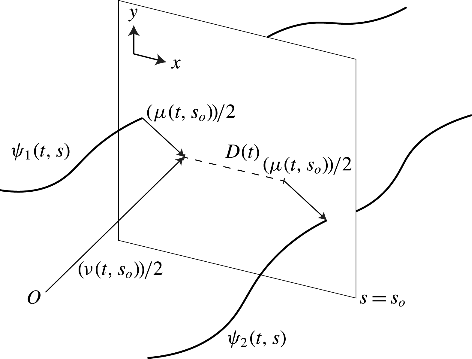
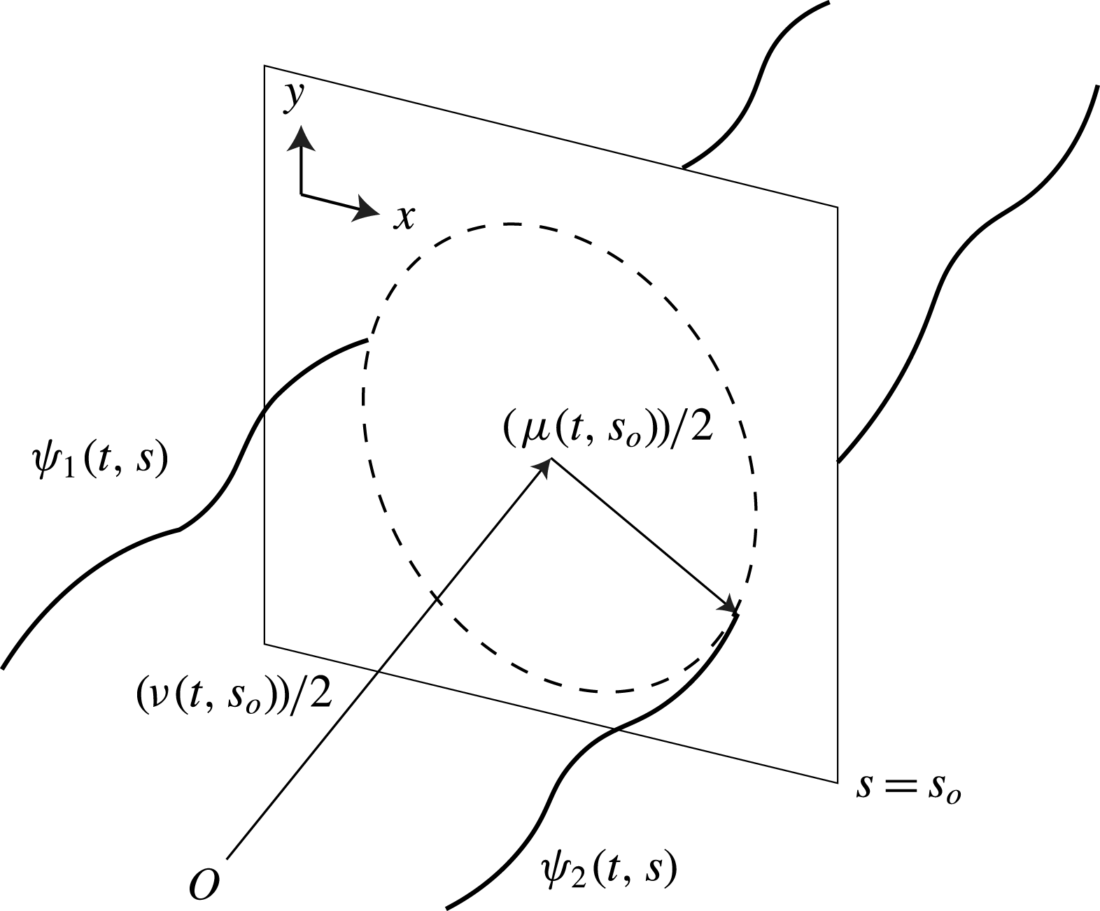
. One can interpret
 $\unicode[STIX]{x1D708}(t,s)$
as the position of the vortex pair centre, while
 $\unicode[STIX]{x1D707}(t,s)$
describes the deviations from this centre with the additional
 $D(t)$
offset (see figure 1). Furthermore, we rescale the independent variables
 ${\hat{s}}=s/\sqrt{\unicode[STIX]{x1D6FC}}$
and
 $\hat{t}=\unicode[STIX]{x1D6E4}_{1}t$
to obtain (upon dropping the hat symbol)
 $$\begin{eqnarray}\displaystyle & \displaystyle \text{i}{\displaystyle \frac{\unicode[STIX]{x2202}\unicode[STIX]{x1D708}}{\unicode[STIX]{x2202}t}}+{\displaystyle \frac{1}{2}}(1+\unicode[STIX]{x1D6F1}){\displaystyle \frac{\unicode[STIX]{x2202}^{2}\unicode[STIX]{x1D708}}{\unicode[STIX]{x2202}s^{2}}}-{\displaystyle \frac{1}{2}}(1-\unicode[STIX]{x1D6F1}){\displaystyle \frac{\unicode[STIX]{x2202}^{2}\unicode[STIX]{x1D707}}{\unicode[STIX]{x2202}s^{2}}}+2(1-\unicode[STIX]{x1D6F1}){\displaystyle \frac{\unicode[STIX]{x1D707}+D}{|\unicode[STIX]{x1D707}+D|^{2}}}=0, & \displaystyle\end{eqnarray}$$
 $$\begin{eqnarray}\displaystyle & \displaystyle \text{i}{\displaystyle \frac{\unicode[STIX]{x2202}\unicode[STIX]{x1D707}}{\unicode[STIX]{x2202}t}}-{\displaystyle \frac{1}{2}}(1-\unicode[STIX]{x1D6F1}){\displaystyle \frac{\unicode[STIX]{x2202}^{2}\unicode[STIX]{x1D708}}{\unicode[STIX]{x2202}s^{2}}}+{\displaystyle \frac{1}{2}}(1+\unicode[STIX]{x1D6F1}){\displaystyle \frac{\unicode[STIX]{x2202}^{2}\unicode[STIX]{x1D707}}{\unicode[STIX]{x2202}s^{2}}}+2(1+\unicode[STIX]{x1D6F1}){\displaystyle \frac{\unicode[STIX]{x1D707}+D}{|\unicode[STIX]{x1D707}+D|^{2}}}=0, & \displaystyle\end{eqnarray}$$
where
 $\unicode[STIX]{x1D6F1}=\unicode[STIX]{x1D6E4}_{2}/\unicode[STIX]{x1D6E4}_{1}$
is the ratio of vortex circulations. It should be noted that in rescaling
 $t$
, we have assumed that
 $\unicode[STIX]{x1D6E4}_{1}>0$
; however, the case of
 $\unicode[STIX]{x1D6E4}_{1}<0$
can readily be accounted for by transforming
 $t\rightarrow -t$
. For the forthcoming analysis, we only consider the former case of
 $\unicode[STIX]{x1D6E4}_{1}>0$
.
A pictorial representation of the transformed dependent variables
 $\unicode[STIX]{x1D708}(t,s)$
and
 $\unicode[STIX]{x1D707}(t,s)$
and how they relate to the original variables
 $\unicode[STIX]{x1D713}_{1}(t,s)$
and
 $\unicode[STIX]{x1D713}_{2}(t,s)$
defined in (2.1) and (2.2). The variable
 $\unicode[STIX]{x1D708}(t,s)$
determines the centre of the vortex pair while
 $\unicode[STIX]{x1D707}(t,s)$
measures the deviations from this centre with an offset
 $D(t)$
.
2.1 Co-rotating vortex pair at large separations
We suppose that the two vortices have the same circulation (i.e.
 $\unicode[STIX]{x1D6F1}=1$
). In this case, (2.3) and (2.4) decouple, meaning that the deviations of an individual vortex filament from the centre and the position of this centre do not depend on each other. The evolution of the vortex pair is now described by
 $$\begin{eqnarray}\displaystyle & \displaystyle \text{i}{\displaystyle \frac{\unicode[STIX]{x2202}\unicode[STIX]{x1D708}}{\unicode[STIX]{x2202}t}}+{\displaystyle \frac{\unicode[STIX]{x2202}^{2}\unicode[STIX]{x1D708}}{\unicode[STIX]{x2202}s^{2}}}=0, & \displaystyle\end{eqnarray}$$
 $$\begin{eqnarray}\displaystyle & \displaystyle \text{i}{\displaystyle \frac{\unicode[STIX]{x2202}\unicode[STIX]{x1D707}}{\unicode[STIX]{x2202}t}}+{\displaystyle \frac{\unicode[STIX]{x2202}^{2}\unicode[STIX]{x1D707}}{\unicode[STIX]{x2202}s^{2}}}+4{\displaystyle \frac{\unicode[STIX]{x1D707}+D}{|\unicode[STIX]{x1D707}+D|^{2}}}=0. & \displaystyle\end{eqnarray}$$
By making the transformation to
 $\unicode[STIX]{x1D708}(t,s)$
and
 $\unicode[STIX]{x1D707}(t,s)$
, we have removed the nonlinear interaction term, leaving us with the linear Schrödinger equation in (2.5). For this reason, we only focus on (2.6) and study the travelling wave and self-similar solutions that result.
2.1.1 Travelling wave solutions
We consider the case where the vortex pair are separated by a constant distance; that is,
 $D(t)=d\gg 1$
, and study travelling wave solutions to (2.6). We do this by introducing the independent variable
 $\unicode[STIX]{x1D709}=s-vt$
, where
 $v$
is the velocity of the travelling wave (which is assumed to be constant and
 $O(1)$
), and find that the transformed equation becomes
 $$\begin{eqnarray}{\displaystyle \frac{\text{d}^{2}\unicode[STIX]{x1D707}}{\text{d}\unicode[STIX]{x1D709}^{2}}}-\text{i}v{\displaystyle \frac{\text{d}\unicode[STIX]{x1D707}}{\text{d}\unicode[STIX]{x1D709}}}+4{\displaystyle \frac{\unicode[STIX]{x1D707}+d}{|\unicode[STIX]{x1D707}+d|^{2}}}=0.\end{eqnarray}$$
We make use of the fact that we are studying large separation distances and expand
 $\unicode[STIX]{x1D707}(\unicode[STIX]{x1D709})$
as a series in
 $d^{-1}$
. In particular,
 $\unicode[STIX]{x1D707}=\sum _{m=0}^{\infty }(d)^{-m}\unicode[STIX]{x1D707}^{(m)}$
, so that the second-order asymptotic solution is (see § A.1.1 for details)
 $$\begin{eqnarray}\displaystyle & & \displaystyle \hspace{-8.00003pt}\unicode[STIX]{x1D707}(t,s)=c_{1}\exp (\text{i}v(s-vt))+c_{2}+{\displaystyle \frac{1}{d}}\left(c_{3}\exp (\text{i}v(s-vt))+c_{4}-{\displaystyle \frac{4\text{i}}{v}}(s-vt)\right)\nonumber\\ \displaystyle & & \displaystyle \hspace{-8.00003pt}\quad +\,{\displaystyle \frac{1}{d^{2}}}\left(-{\displaystyle \frac{2c_{1}^{\ast }}{v^{2}}}\exp (-\text{i}v(s-vt))+{\displaystyle \frac{4\text{i}c_{2}^{\ast }}{v}}(s-vt)+c_{5}\exp (\text{i}v(s-vt))+c_{6}\right)+O\!\left({\displaystyle \frac{1}{d^{3}}}\right)\!,\nonumber\\ \displaystyle & & \displaystyle\end{eqnarray}$$
where
 $c_{n}\in \mathbb{C}$
are integration constants and
 $(~)^{\ast }$
is the complex conjugate of the variable.
Equation (2.8) suggests that if the vortices are held at infinite separation, such that only self-induction effects are included, the resulting shape of the individual filaments is that of a helix with wavenumber
 $v$
that oscillates at an angular frequency of
 $v^{2}$
. As the pair is brought closer together, the vortex interaction is manifested in two ways. First, there is repulsion in the perpendicular direction due to the
 $-4\text{i}(s-vt)/v$
term, which is independent of any imposed conditions on
 $\unicode[STIX]{x1D707}(\unicode[STIX]{x1D709})$
; an expected result in light of point vortices. In a 2D flow, each co-rotating point vortex will feel a velocity field that is opposite in direction to the field felt by the other vortex, both of which are perpendicular to the direction of separation, thus driving the pair apart in the same manner as equation (2.8) predicts. Noting that
 $\unicode[STIX]{x1D6E4}_{1}=\unicode[STIX]{x1D6E4}_{2}>0$
, the direction of repulsion is such that the filament described by
 $\unicode[STIX]{x1D713}_{1}(t,s)$
will drift in the positive
 $y$
direction while the filament described by
 $\unicode[STIX]{x1D713}_{2}(t,s)$
will drift in the negative
 $y$
direction. If we consider the case where
 $\unicode[STIX]{x1D6E4}_{1}<0$
, such that
 $t\rightarrow -t$
, the vortices are repelled in the opposite direction along the
 $y$
-axis.
Second, an additional wave is generated in the configuration as a response to the zeroth-order solution; one that has the form
 $-2c_{1}^{\ast }\text{exp}(-\text{i}v\unicode[STIX]{x1D709})/v$
. If we suppose that
 $\text{Im}(c_{1})=0$
, then for
 $\text{Re}(c_{1})>0$
, the secondary wave suppresses oscillations in the
 $y$
direction, while vibrations in the
 $x$
direction are similarly subdued when
 $\text{Re}(c_{1})<0$
. Physically, the helical shapes of the filaments flatten into ellipses due to the pairwise vortex interaction.
Furthermore, there is additional attraction or repulsion at
 $O(d^{-2})$
that depends on the initial offset of the helical vortices; that is, it depends on
 $4\text{i}c_{2}^{\ast }\unicode[STIX]{x1D709}/v$
. An offset that is in the
 $x$
direction results in repulsion in the
 $y$
direction, as seen in the first-order correction. However, if the constant offset is in the
 $y$
direction, then the opposite holds true; namely, the vortex pair is translated in the
 $x$
direction in either repulsion or attraction. For
 $\unicode[STIX]{x1D6E4}_{1}>0$
, if
 $\text{Im}(c_{2})>0$
, then
 $4\text{i}c_{2}^{\ast }\unicode[STIX]{x1D709}/v>0$
and the pair attract each other, while if
 $\text{Im}(c_{2})<0$
, then
 $4\text{i}c_{2}^{\ast }\unicode[STIX]{x1D709}/v<0$
and the vortices repel each other. The opposite applies when
 $\unicode[STIX]{x1D6E4}_{1}<0$
. This secondary repulsion or attraction is not predicted by the 2D theory and is a consequence of the vortex filaments existing in a 3D flow.
We numerically solve (2.7) for the parameters
 $v=4$
and
 $d=10$
, with initial conditions
 $\unicode[STIX]{x1D707}(\unicode[STIX]{x1D709}=0)=-\text{i}$
and
 $\unicode[STIX]{x1D707}^{\prime }(\unicode[STIX]{x1D709}=0)=v$
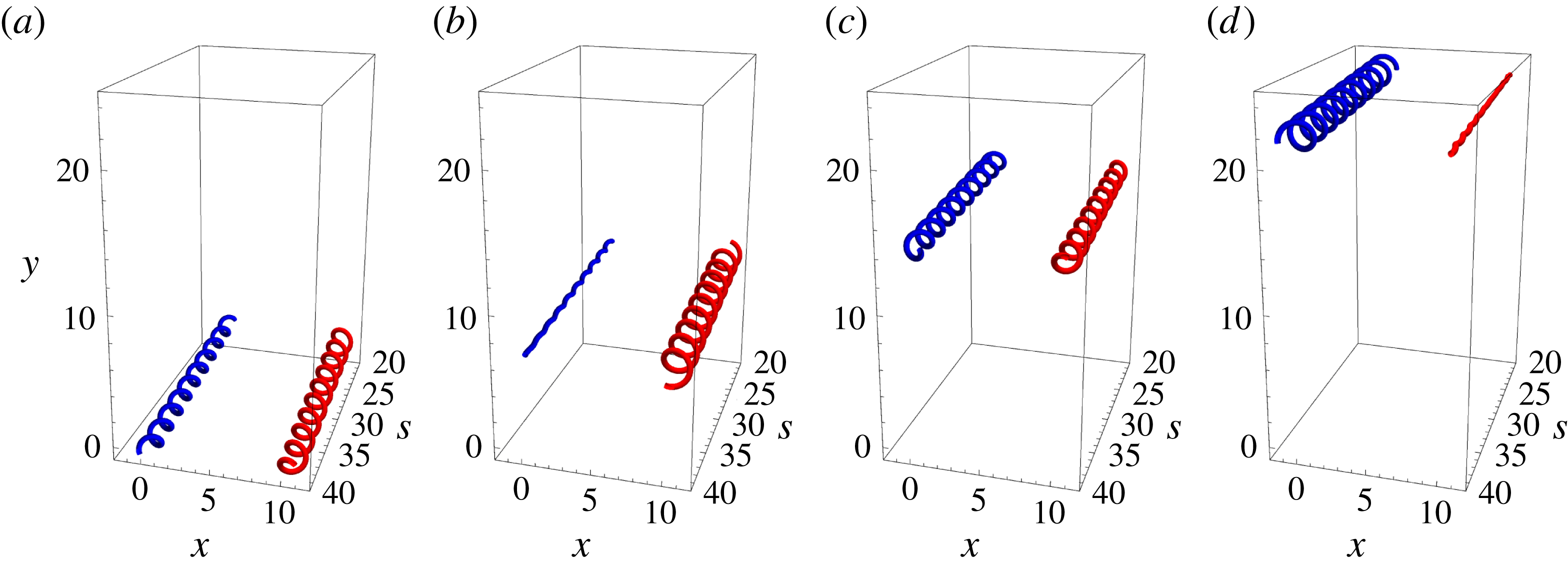
, and plot the vortex filament shapes that result when we set
 $\unicode[STIX]{x1D708}(t,s)=0$
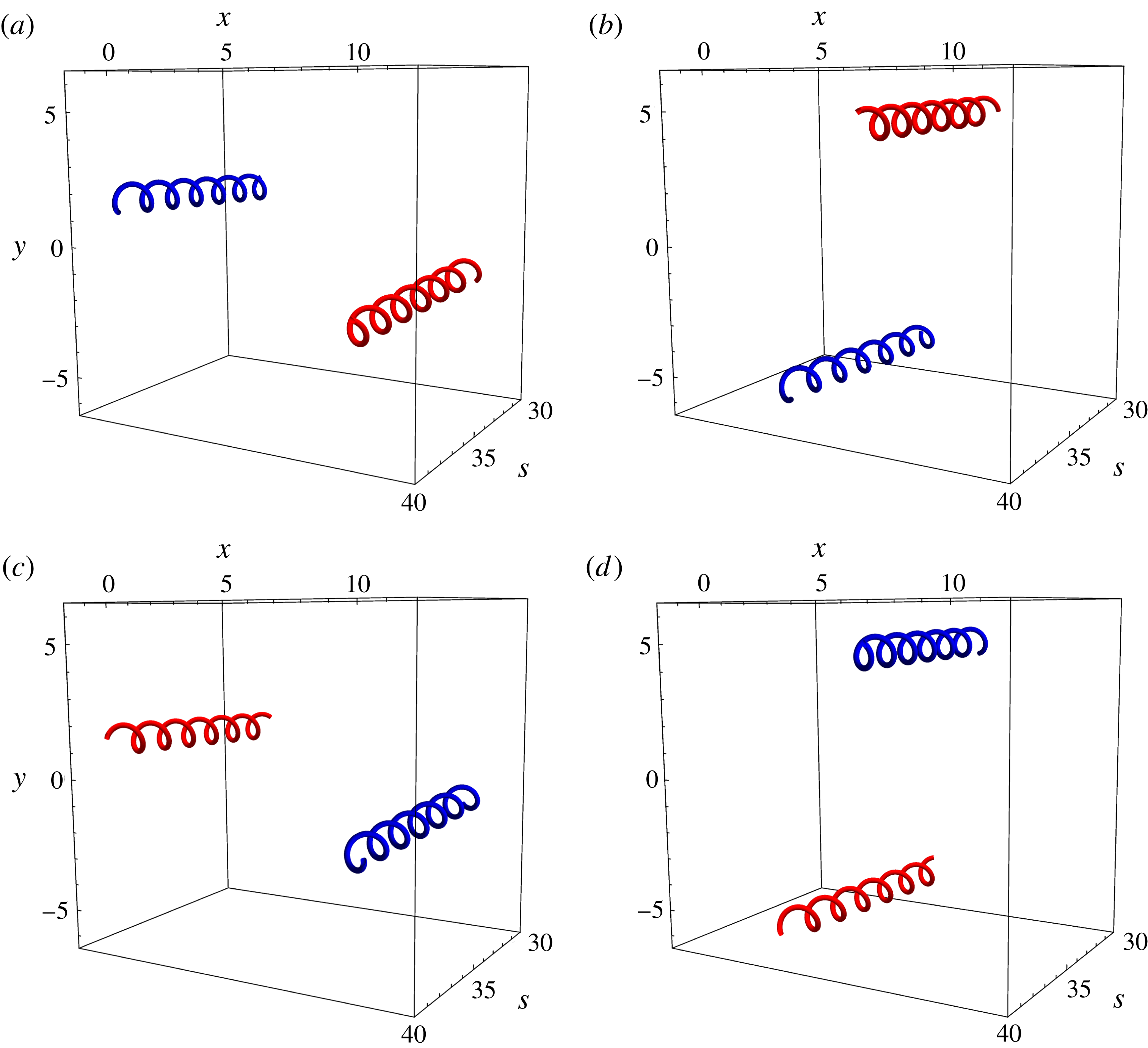
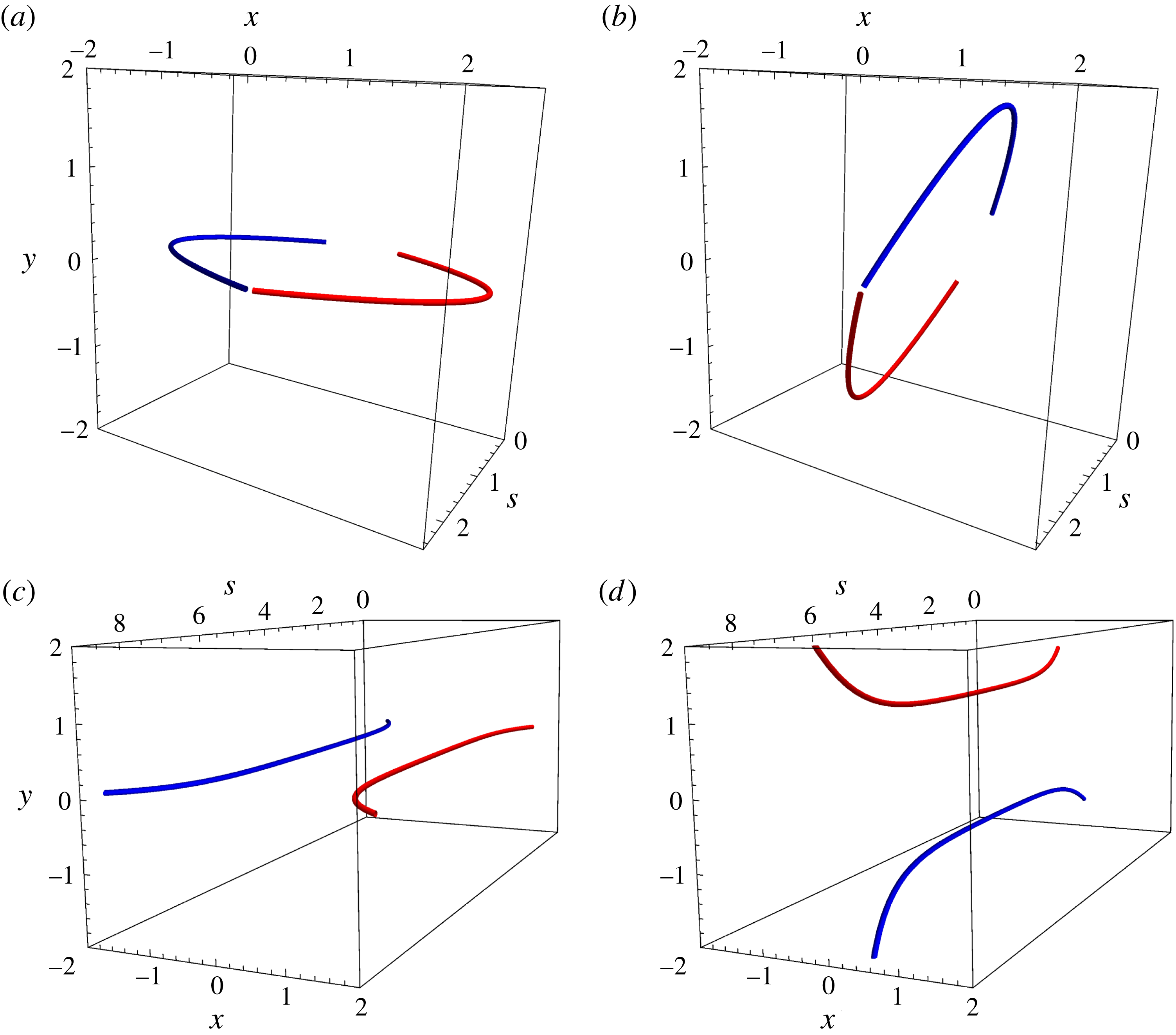
(shown in figure 2(a–d) for times
 $t=\{0,40,80,120\}$
respectively). We observe that (2.8) breaks down for times past the initial repulsion of the vortex pair and does not capture the slowly oscillatory behaviour of the numerical solution. This periodic solution on the slow wave scale physically corresponds to the binary orbit of the vortex pair, whereby the filaments rotate around each other (see figure 2). This result is predicted if one considers the same problem from the perspective of 2D vortices. As the vortices separate vertically from their initial repulsion (figure 2
a), the velocity field felt by each vortex becomes increasingly horizontal and decreasingly vertical, resulting in the pair becoming vertically displaced from each other (figure 2
b). The velocity field for each vortex is now horizontal, with the repulsion now leading to increasing vertical contributions and decreasing horizontal contributions in the velocity. The pair become horizontally separated again (figure 2
c) and the cycle repeats.
Given that the pair are orbiting on a slow wave scale and are separated by a constant
 $d$
through all orientations, we instead look for a slowly varying solution of the form
 $$\begin{eqnarray}1+{\displaystyle \frac{1}{d}}\unicode[STIX]{x1D707}_{\mathit{slow}}(\unicode[STIX]{x1D709})=\exp \left({\displaystyle \frac{\text{i}\unicode[STIX]{x1D703}(\unicode[STIX]{x1D709})}{d^{\unicode[STIX]{x1D6FD}}}}\right),\end{eqnarray}$$
where
 $\unicode[STIX]{x1D6FD}$
is a positive constant and
 $\unicode[STIX]{x1D6FD},\unicode[STIX]{x1D703}\in \mathbb{R}$
. Ansatz (2.9) replaces the helical shape of each vortex in the pair, which individually rotate on a fast time scale, with straight filaments that no longer exhibit fast oscillations.
Substituting (2.9) into (2.7), we find the general solution (see § A.1.2 for details)
 $$\begin{eqnarray}\unicode[STIX]{x1D703}(\unicode[STIX]{x1D709})=dc_{7}-{\displaystyle \frac{4\unicode[STIX]{x1D709}}{v}}+c_{8}+{\displaystyle \frac{c_{9}}{d}}+O\left({\displaystyle \frac{1}{d^{3}}}\right),\end{eqnarray}$$
where
 $c_{7},c_{8},c_{9}\in \mathbb{R}$
are integration constants determining the initial orientation of the vortex pair. The odd powers of
 $d^{-n}$
in (2.10) are corrections so that (2.9) satisfies the initial conditions imposed on
 $\unicode[STIX]{x1D707}_{\mathit{slow}}(\unicode[STIX]{x1D709})$
, while even powers give corrections to the frequency of the vortex pair orbit.
We compare
 $\unicode[STIX]{x1D707}_{\mathit{slow}}(\unicode[STIX]{x1D709})$
in (2.9), with
 $\unicode[STIX]{x1D703}(\unicode[STIX]{x1D709})$
calculated from (2.10), with the numerical solution of (2.7) for the same initial conditions and value for
 $v$
as seen previously. To impose
 $\unicode[STIX]{x1D707}_{\mathit{slow}}(\unicode[STIX]{x1D709}=0)=-\text{i}$
, we expand the exponential in (2.9) as a series and match powers of
 $d^{-1}$
on both sides, giving
 $c_{7}=-1$
,
 $c_{8}=0$
and
 $c_{9}=0$
, which incurs an error of
 $O(d^{-2})$
at
 $\unicode[STIX]{x1D709}=0$
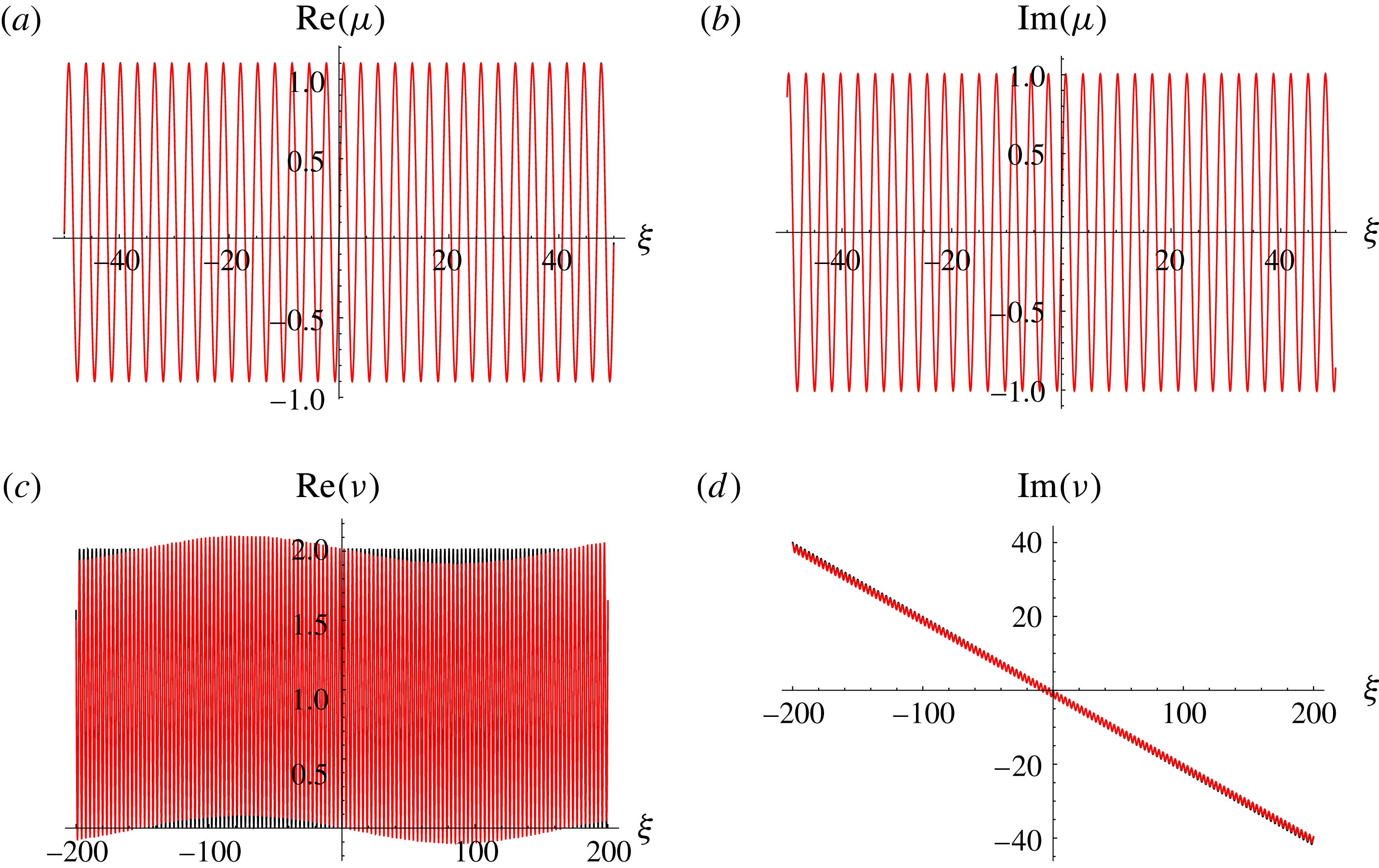
. We show these comparisons for
 $d=10$
in figure 3(a,b) and
 $d=5$
in figure 3(c,d) for the real and imaginary parts of
 $\unicode[STIX]{x1D707}(\unicode[STIX]{x1D709})$
. We observe that the slowly varying approximation agrees very well with the numerical solutions showing the vortex pair binary orbit, even for
 $d=5$
. However, we note that (2.9) and (2.10) begin to break down as
 $\unicode[STIX]{x1D709}\approx 2000$
, suggesting that higher-order frequency corrections are necessary to keep this solution valid for large
 $\unicode[STIX]{x1D709}$
.
The time evolution of travelling wave solutions in co-rotating vortices held at a constant distance, with
 $\unicode[STIX]{x1D713}_{1}(t,s)$
and
 $\unicode[STIX]{x1D713}_{2}(t,s)$
being denoted by blue and red respectively. In particular,
 $\unicode[STIX]{x1D708}(t,s)=0$
and the numerical solution to (2.7) have been plotted with initial conditions
 $\unicode[STIX]{x1D707}(\unicode[STIX]{x1D709}=0)=-\text{i}$
and
 $\unicode[STIX]{x1D707}^{\prime }(\unicode[STIX]{x1D709}=0)=v$
, for
 $v=4$
and
 $d=10$
, over
 $s\in [30,40]$
. The times shown are (a)
 $t=0$
, (b)
 $t=40$
, (c)
 $t=80$
and (d)
 $t=120$
.
Real and imaginary components of
 $\unicode[STIX]{x1D707}(\unicode[STIX]{x1D709})$
for the slowly varying solution (2.9) and (2.10) (denoted by black) and numerical solution of the full problem (2.7) (denoted by red). The initial conditions imposed are
 $\unicode[STIX]{x1D707}(\unicode[STIX]{x1D709}=0)=-\text{i}$
and
 $\unicode[STIX]{x1D707}^{\prime }(\unicode[STIX]{x1D709}=0)=v$
for parameters
 $v=4$
and (a,b)
 $d=10$
and (c,d)
 $d=5$
.

2.1.2 Self-similar solutions
We consider the case where the separation of the vortex pair grows in time; that is,
 $D(t)=d\sqrt{t}$
. As in § 2.1.1,
 $d\in \mathbb{R}$
is a constant that is very large such that
 $1/d=\unicode[STIX]{x1D716}\ll 1$
. For a vortex separation of this form, equation (2.6) has self-similar solutions given by
 $\unicode[STIX]{x1D707}(t,s)=\sqrt{t}\unicode[STIX]{x1D712}(\unicode[STIX]{x1D702})$
, where
 $\unicode[STIX]{x1D702}=s/\sqrt{t}$
. Transforming so that
 $\unicode[STIX]{x1D702}$
is the independent variable, (2.6) becomes
 $$\begin{eqnarray}{\displaystyle \frac{\text{d}^{2}\unicode[STIX]{x1D712}}{\text{d}\unicode[STIX]{x1D702}^{2}}}-{\displaystyle \frac{\text{i}\unicode[STIX]{x1D702}}{2}}{\displaystyle \frac{\text{d}\unicode[STIX]{x1D712}}{\text{d}\unicode[STIX]{x1D702}}}+{\displaystyle \frac{\text{i}}{2}}\unicode[STIX]{x1D712}+4{\displaystyle \frac{\unicode[STIX]{x1D712}+d}{|\unicode[STIX]{x1D712}+d|^{2}}}=0.\end{eqnarray}$$
Taking
 $d^{-1}\ll 1$
, we expand
 $\unicode[STIX]{x1D712}(\unicode[STIX]{x1D702})$
as a power series in
 $d^{-1}$
, so that
 $\unicode[STIX]{x1D712}(\unicode[STIX]{x1D702})=\sum _{n=0}^{\infty }d^{-n}\unicode[STIX]{x1D712}^{(n)}$
, to find the first-order asymptotic solution (see § A.2)
 $$\begin{eqnarray}\displaystyle & & \displaystyle \unicode[STIX]{x1D707}(t,s)=(-1)^{1/4}a_{1}s+a_{2}\left(\sqrt{t}\text{exp}\left({\displaystyle \frac{\text{i}s^{2}}{4t}}\right)-{\displaystyle \frac{(-1)^{1/4}\sqrt{\unicode[STIX]{x03C0}}}{2}}s\text{erfi}\left({\displaystyle \frac{(-1)^{1/4}s}{2\sqrt{t}}}\right)\!\right)\nonumber\\ \displaystyle & & \displaystyle \qquad +\,{\displaystyle \frac{1}{d}}\!\left(8\text{i}\sqrt{t}+(-1)^{1/4}a_{3}s+a_{4}\!\left(\!\sqrt{t}\text{exp}\left({\displaystyle \frac{\text{i}s^{2}}{4t}}\right)+{\displaystyle \frac{(-1)^{3/4}\sqrt{\unicode[STIX]{x03C0}}}{2}}s\text{erf}\left({\displaystyle \frac{(-1)^{3/4}s}{2\sqrt{t}}}\right)\!\right)\!\right)\nonumber\\ \displaystyle & & \displaystyle \qquad +\,O\left({\displaystyle \frac{1}{d^{2}}}\right),\end{eqnarray}$$
where
 $a_{n}\in \mathbb{C}$
are integration constants and
 $\text{erfi}(z)=\text{i}\text{erf}(\text{i}z)$
is the complex error function.
We plot the vortex filament shapes obtained by numerically solving (2.11) for
 $\unicode[STIX]{x1D712}(\unicode[STIX]{x1D702}=100)=1+\text{i}$
,
 $\unicode[STIX]{x1D712}^{\prime }(\unicode[STIX]{x1D702}=100)=1$
and
 $d=10$
with
 $\unicode[STIX]{x1D708}(t,s)=0$
for times
 $t=\{0.1,0.5,1,2\}$
in figure 4. These conditions correspond to
 $\unicode[STIX]{x1D707}(t,s)$
having an initial shape that satisfies the relations
 $$\begin{eqnarray}\displaystyle & \displaystyle \left.\left(-{\displaystyle \frac{2t^{3/2}}{s}}{\displaystyle \frac{\unicode[STIX]{x2202}\unicode[STIX]{x1D707}}{\unicode[STIX]{x2202}t}}+t^{1/2}{\displaystyle \frac{\unicode[STIX]{x2202}\unicode[STIX]{x1D707}}{\unicode[STIX]{x2202}s}}\right)\right|_{\begin{smallmatrix}t=t_{0}\\ s=s_{0}\end{smallmatrix}}=1, & \displaystyle\end{eqnarray}$$
 $$\begin{eqnarray}\displaystyle & \displaystyle \unicode[STIX]{x1D707}(t_{0},s_{0})=\sqrt{t_{0}}(1+\text{i}), & \displaystyle\end{eqnarray}$$
evaluated at
 $100=s_{0}/\sqrt{t_{0}}$
.
The time evolution of self-similar solutions in co-rotating vortices held apart by a separation function
 $D(t)=\sqrt{t}$
, with
 $\unicode[STIX]{x1D713}_{1}(t,s)$
and
 $\unicode[STIX]{x1D713}_{2}(t,s)$
being denoted by blue and red respectively. In particular,
 $\unicode[STIX]{x1D708}(t,s)=0$
and (2.11), with conditions satisfying (2.13) and (2.14), have been plotted for
 $d=10$
over
 $s\in [10,20]$
. The times shown are (a)
 $t=0.1$
, (b)
 $t=0.5$
, (c)
 $t=1$
and (d)
 $t=2$
.

Solutions of
 $\unicode[STIX]{x1D712}(\unicode[STIX]{x1D702})$
calculated from the first-order asymptotic solution (2.12) (shown in black) and the numerical solution of (2.11) (shown in red). In particular, the initial conditions
 $\unicode[STIX]{x1D712}(\unicode[STIX]{x1D702}=100)=1+\text{i}$
and
 $\unicode[STIX]{x1D712}^{\prime }(\unicode[STIX]{x1D702}=100)=1$
were used with
 $d=10$
.
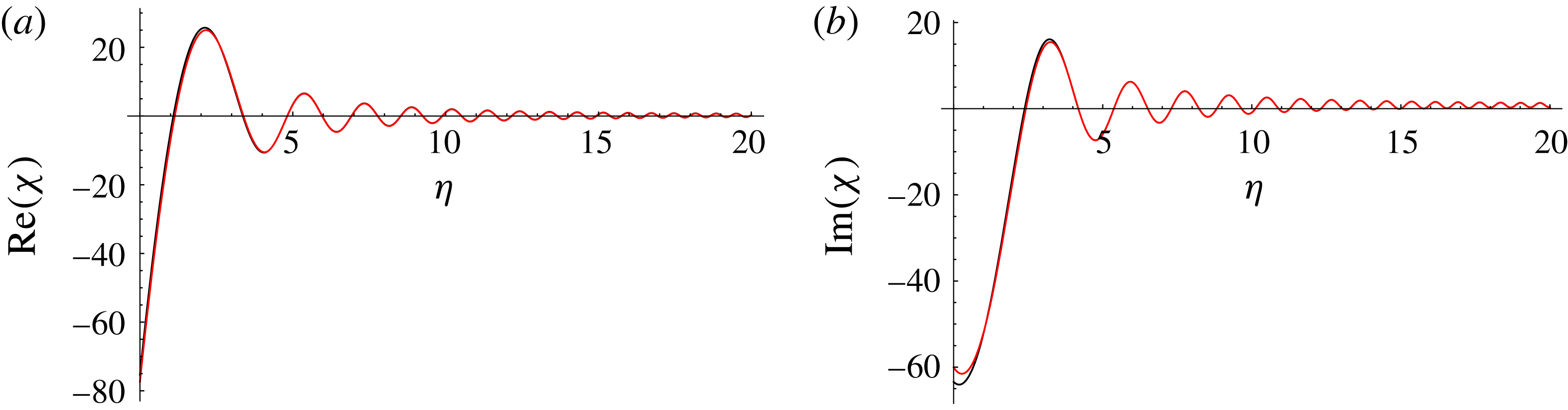
We further compare the numerical solution with the asymptotic solution in (2.12) for the same boundary conditions in figure 5 and describe the form of solutions predicted for
 $t>0$
and
 $s>0$
as follows. At zeroth order, the initial shape of the pair is that of individual helical cones along an arbitrary orientation whose amplitude, wavelength and separation grow with time. The conical nature of the helix arises from the complex error function, while the increasing helix amplitude is due to the complex exponential in (2.12). Such conical-type solutions were previously seen for isolated vortex filaments (Van Gorder Reference Van Gorder2016). The inclusion of vortex interaction at first order gives the same general shape as the zeroth-order solution, with the exception of the monotonically increasing term in
 $\sqrt{t}$
. As in § 2.1.1, the vortex pair exhibit repulsion in opposite directions along the
 $y$
-axis; however, in this instance, the asymptotic solution does not show significant disagreement with the numerical solution for
 $t\rightarrow \infty$
. This is due to the separation function
 $D(t)$
used, which makes binary orbits, as seen with travelling wave solutions, impossible due to the horizontal distance between the vortex pair increasing with time rather than staying constant. Finally, we note that the rotation of the vortex helices is such that they rotate in the same direction, with the orientation of one helix being a reflection of the other in both the
 $x$
- and the
 $y$
-axes. In figure 4, both vortices have circulation
 $\unicode[STIX]{x1D6E4}>0$
; however, the helices rotate in a clockwise direction, suggesting that the direction of a helix rotation is opposite to an individual filament circulation.
2.2 Counter-rotating vortex pair at large separations
For a vortex pair with opposite circulation,
 $\unicode[STIX]{x1D6F1}=-1$
, so that (2.3) and (2.4) now give
 $$\begin{eqnarray}\displaystyle & \displaystyle \text{i}{\displaystyle \frac{\unicode[STIX]{x2202}\unicode[STIX]{x1D708}}{\unicode[STIX]{x2202}t}}-{\displaystyle \frac{\unicode[STIX]{x2202}^{2}\unicode[STIX]{x1D707}}{\unicode[STIX]{x2202}s^{2}}}+4{\displaystyle \frac{\unicode[STIX]{x1D707}+D}{|\unicode[STIX]{x1D707}+D|^{2}}}=0, & \displaystyle\end{eqnarray}$$
 $$\begin{eqnarray}\displaystyle & \displaystyle \text{i}{\displaystyle \frac{\unicode[STIX]{x2202}\unicode[STIX]{x1D707}}{\unicode[STIX]{x2202}t}}-{\displaystyle \frac{\unicode[STIX]{x2202}^{2}\unicode[STIX]{x1D708}}{\unicode[STIX]{x2202}s^{2}}}=0. & \displaystyle\end{eqnarray}$$
However, supposing that
 $\unicode[STIX]{x1D713}_{1}(t,s)$
and
 $\unicode[STIX]{x1D713}_{2}(t,s)$
are
 $C^{4}$
in
 $s$
and
 $C^{2}$
in
 $t$
, we differentiate (2.16) once with respect to
 $t$
and differentiate (2.15) twice with respect to
 $s$
to find a single time-evolution equation for
 $\unicode[STIX]{x1D707}(t,s)$
,
 $$\begin{eqnarray}{\displaystyle \frac{\unicode[STIX]{x2202}^{2}\unicode[STIX]{x1D707}}{\unicode[STIX]{x2202}t^{2}}}+{\displaystyle \frac{\unicode[STIX]{x2202}^{4}\unicode[STIX]{x1D707}}{\unicode[STIX]{x2202}s^{4}}}-4{\displaystyle \frac{\unicode[STIX]{x2202}^{2}}{\unicode[STIX]{x2202}s^{2}}}\left({\displaystyle \frac{\unicode[STIX]{x1D707}+D}{|\unicode[STIX]{x1D707}+D|^{2}}}\right)=0,\end{eqnarray}$$
which has similarities with equations in the studies of beams and cables (Lazer & McKenna Reference Lazer and McKenna1990).
There are two noteworthy aspects of (2.17). First,
 $\unicode[STIX]{x1D707}(t,s)$
and
 $\unicode[STIX]{x1D708}(t,s)$
are not independent of each other and are still related by (2.16); that is, the position of the vortex pair centre and the deviations from this centre are coupled, unlike the co-rotating vortices studied in § 2.1. Second, the additional conditions necessary to solve (2.17) now come from those that are imposed on
 $\unicode[STIX]{x1D708}(t,s)$
, along with its relation to
 $\unicode[STIX]{x1D707}(t,s)$
, according to (2.15) and (2.16).
2.2.1 Travelling wave solutions
As in § 2.1.1, we consider vortices that are separated by a constant distance
 $D(t)=d$
such that we have the small parameter
 $d^{-1}\ll 1$
. Transforming (2.17) into wave coordinates
 $\unicode[STIX]{x1D709}=s-vt$
, with
 $v=O(1)$
, we find
 $$\begin{eqnarray}{\displaystyle \frac{\text{d}^{2}\unicode[STIX]{x1D707}}{\text{d}\unicode[STIX]{x1D709}^{2}}}+v^{2}\unicode[STIX]{x1D707}-4{\displaystyle \frac{\unicode[STIX]{x1D707}+d}{|\unicode[STIX]{x1D707}+d|^{2}}}=\unicode[STIX]{x1D6FF},\end{eqnarray}$$
where there is only one non-zero integration constant due to the relationship between
 $\unicode[STIX]{x1D707}(t,s)$
and
 $\unicode[STIX]{x1D708}(t,s)$
, which imposes the constraints
 $$\begin{eqnarray}\displaystyle & \displaystyle {\displaystyle \frac{\text{d}^{3}\unicode[STIX]{x1D707}}{\text{d}\unicode[STIX]{x1D709}^{3}}}+v^{2}{\displaystyle \frac{\text{d}\unicode[STIX]{x1D707}}{\text{d}\unicode[STIX]{x1D709}}}-4{\displaystyle \frac{\text{d}}{\text{d}\unicode[STIX]{x1D709}}}\left({\displaystyle \frac{\unicode[STIX]{x1D707}+d}{|\unicode[STIX]{x1D707}+d|^{2}}}\right)=0, & \displaystyle\end{eqnarray}$$
 $$\begin{eqnarray}\displaystyle & \displaystyle v^{2}\unicode[STIX]{x1D707}-\text{i}v{\displaystyle \frac{\text{d}\unicode[STIX]{x1D708}}{\text{d}\unicode[STIX]{x1D709}}}=\unicode[STIX]{x1D6FF}, & \displaystyle\end{eqnarray}$$
with the latter equation used to determine
 $\unicode[STIX]{x1D6FF}$
from conditions on
 $\unicode[STIX]{x1D707}(\unicode[STIX]{x1D709})$
and
 $\unicode[STIX]{x1D708}^{\prime }(\unicode[STIX]{x1D709})$
.
We note that (2.18) has solutions up to
 $O(d^{-2})$
that remain finite for all time and along the entire arclength of the filament pair, provided that the velocity of the travelling wave
 $v$
is such that
 $v^{2}>4d^{-2}$
. As a result, we are able to find solutions of the oscillatory Poincaré–Lindstedt form, which, to second order, are
 $$\begin{eqnarray}\displaystyle X(\unicode[STIX]{x1D6EF}_{1}) & = & \displaystyle c_{1}\cos (v\unicode[STIX]{x1D6EF}_{1})+c_{2}\sin (v\unicode[STIX]{x1D6EF}_{1})+{\displaystyle \frac{\unicode[STIX]{x1D6FF}_{1}}{v^{2}}}+{\displaystyle \frac{1}{d}}\left(c_{3}\cos (v\unicode[STIX]{x1D6EF}_{1})+c_{4}\sin (v\unicode[STIX]{x1D6EF}_{1})+{\displaystyle \frac{4}{v^{2}}}\right)\nonumber\\ \displaystyle & & \displaystyle +\,{\displaystyle \frac{1}{d^{2}}}\left(c_{5}\cos (v\unicode[STIX]{x1D6EF}_{1})+c_{6}\sin (v\unicode[STIX]{x1D6EF}_{1})-{\displaystyle \frac{4\unicode[STIX]{x1D6FF}_{1}}{v^{4}}}\right)\end{eqnarray}$$
and
 $$\begin{eqnarray}\displaystyle Y(\unicode[STIX]{x1D6EF}_{2}) & = & \displaystyle c_{7}\cos (v\unicode[STIX]{x1D6EF}_{2})+c_{8}\sin (v\unicode[STIX]{x1D6EF}_{2})+{\displaystyle \frac{\unicode[STIX]{x1D6FF}_{2}}{v^{2}}}+{\displaystyle \frac{1}{d}}(c_{9}\cos (v\unicode[STIX]{x1D6EF}_{2})+c_{10}\sin (v\unicode[STIX]{x1D6EF}_{2}))\nonumber\\ \displaystyle & & \displaystyle +\,{\displaystyle \frac{1}{d^{2}}}\left(c_{11}\cos (v\unicode[STIX]{x1D6EF}_{2})+c_{12}\sin (v\unicode[STIX]{x1D6EF}_{2})+{\displaystyle \frac{4\unicode[STIX]{x1D6FF}_{2}}{v^{4}}}\right),\end{eqnarray}$$
where
 $X,Y\in \mathbb{R}$
and are related to
 $\unicode[STIX]{x1D707}$
by
 $\unicode[STIX]{x1D707}=X+\text{i}Y$
,
 $\unicode[STIX]{x1D6EF}_{1}=(1+2/v^{2}d^{2})(s-vt)$
,
 $\unicode[STIX]{x1D6EF}_{2}=(1-2/v^{2}d^{2})(s-vt)$
,
 $\unicode[STIX]{x1D6FF}=\unicode[STIX]{x1D6FF}_{1}+\text{i}\unicode[STIX]{x1D6FF}_{2}$
, and all
 $c_{n}\in \mathbb{R}$
(see § A.3.1 for further details).
We comment on some important aspects of (2.21) and (2.22). For counter-rotating vortices, there is no secular vortex repulsion or attraction, unlike what was previously seen with the co-rotating pair in (2.8). Instead, the deviations of the vortex pair have a constant offset, which is determined by the speed of the travelling wave solution, as well as
 $\unicode[STIX]{x1D6FF}$
, which is dependent on the conditions imposed on
 $\unicode[STIX]{x1D707}(\unicode[STIX]{x1D709})$
and
 $\unicode[STIX]{x1D708}^{\prime }(\unicode[STIX]{x1D709})$
. However, we note that by integrating (2.20), the constant offsets seen in
 $\unicode[STIX]{x1D707}(\unicode[STIX]{x1D709})$
become secular in
 $\unicode[STIX]{x1D709}$
for
 $\unicode[STIX]{x1D708}(\unicode[STIX]{x1D709})$
. Although the deviations of the vortex pair may not grow for all time by means of attraction or repulsion, the centre of the vortex pair will move from its initial position; that is, the filaments will move together at a constant velocity through the 3D flow. However, the deviations in the
 $y$
direction will tend to
 $-\infty$
and
 $\infty$
if
 $v^{2}<4\unicode[STIX]{x1D716}^{2}$
, which suggests that the velocity of the travelling wave serves to stabilise the vortex pair so that they remain together. It should be noted that (2.21) and (2.22) will not approximate such a regime accurately because of the assumption made at the beginning of § 2.2.1, namely that
 $v=O(1)$
.
Finally, the oscillation of the filaments is subject to dispersion that arises from the vortex interaction at
 $O(1/d^{2})$
. Vibrations in the
 $x$
direction will increase in frequency by a factor of
 $2/v^{2}d^{2}$
while oscillations in
 $y$
will decrease by
 $2/v^{2}d^{2}$
. This orientation-dependent oscillation causes a vortical helix to shear to a planar vibration and back to a helix again.
To illustrate some of the phenomena outlined, we solve (2.18) and (2.20) numerically for
 $d=10$
and
 $v=1$
with the initial conditions
 $\unicode[STIX]{x1D707}(\unicode[STIX]{x1D709}=0)=0$
,
 $\unicode[STIX]{x1D707}^{\prime }(\unicode[STIX]{x1D709}=0)=v+\text{i}v$
,
 $\unicode[STIX]{x1D708}(\unicode[STIX]{x1D709}=0)=0$
and
 $\unicode[STIX]{x1D708}^{\prime }(\unicode[STIX]{x1D709}=0)=0$
. The corresponding vortex filament shapes are shown in figure 6(a–d) for times
 $t=\{25,80,135,190\}$
respectively. In this case, the inclusion of
 $\unicode[STIX]{x1D708}(t,s)$
causes the vortex pair to travel together in the
 $y$
direction as
 $t>0$
. This result is again predicted by considering the simpler problem of point vortices in a 2D flow. A pair that has opposite circulation will generate a velocity field that is the same direction for both vortices, thus pushing them together. For the case shown in figure 6,
 $\unicode[STIX]{x1D713}_{1}(t,s)$
has positive circulation while
 $\unicode[STIX]{x1D713}_{2}$
has negative circulation, leading to the respective vortices feeling a velocity field that is in the positive
 $y$
direction.
The time evolution of travelling wave solutions in counter-rotating vortices held apart by a constant distance
 $d$
, with
 $\unicode[STIX]{x1D713}_{1}(t,s)$
and
 $\unicode[STIX]{x1D713}_{2}(t,s)$
being denoted by blue and red respectively. In particular, numerical solutions to (2.18) and (2.20) are plotted for
 $v=2$
,
 $d=10$
and initial conditions
 $\unicode[STIX]{x1D707}(\unicode[STIX]{x1D709}=0)=0$
,
 $\unicode[STIX]{x1D707}^{\prime }(\unicode[STIX]{x1D709}=0)=v+\text{i}v$
,
 $\unicode[STIX]{x1D708}(\unicode[STIX]{x1D709}=0)=0$
and
 $\unicode[STIX]{x1D708}^{\prime }(\unicode[STIX]{x1D709}=0)=0$
over
 $s\in [20,40]$
. The times shown are (a)
 $t=25$
, (b)
 $t=80$
, (c)
 $t=135$
and (d)
 $t=190$
.
Real and imaginary components of
 $\unicode[STIX]{x1D707}(\unicode[STIX]{x1D709})$
and
 $\unicode[STIX]{x1D708}(\unicode[STIX]{x1D709})$
predicted by the second-order asymptotic correction (2.21) and (2.22) (shown in black) and numerical solutions of (2.18) and (2.20) (shown in red), with the parameters
 $v=2$
and
 $d=10$
and initial conditions
 $\unicode[STIX]{x1D707}(\unicode[STIX]{x1D709}=0)=0$
,
 $\unicode[STIX]{x1D707}^{\prime }(\unicode[STIX]{x1D709}=0)=v+\text{i}v$
,
 $\unicode[STIX]{x1D708}(\unicode[STIX]{x1D709}=0)=0$
and
 $\unicode[STIX]{x1D708}^{\prime }(\unicode[STIX]{x1D709}=0)=0$
.
However, there is an additional effect that is not predicted by the 2D theory; that is, the oscillations of
 $\unicode[STIX]{x1D708}(t,s)$
. These vibrations cause the amplitude of the helices to periodically vary in a manner such that the individual helices are out of phase with each other. We observe that as time evolves,
 $\unicode[STIX]{x1D713}_{1}(t,s)$
, which initially has a helical shape (figure 6
a), has an amplitude that shrinks (figure 6
b), before returning to its original shape (figure 6
c). The vortex described by
 $\unicode[STIX]{x1D713}_{2}(t,s)$
is out of phase in that its amplitude shrinks when
 $\unicode[STIX]{x1D713}_{1}(t,s)$
grows (figure 6
d).
We compare the asymptotic solutions given by (2.21) and (2.22) with the numerical solution of (2.18) for the same parameters and initial conditions on
 $\unicode[STIX]{x1D707}(\unicode[STIX]{x1D709})$
and
 $\unicode[STIX]{x1D708}(\unicode[STIX]{x1D709})$
(shown in figure 7). We note that the asymptotic solutions provide a very good approximation to the full vortex interaction, with a notable exception: the solution with the untruncated vortex interaction predicts that
 $\unicode[STIX]{x1D708}(\unicode[STIX]{x1D709})$
exhibits slow amplitude modulation when compared with the second-order asymptotic correction in figure 7(c). This result suggests that, in a similar manner to that for the co-rotating vortices, we require a slow-scale analysis of the problem to capture this effect.
We look for a slow solution of the form
 $$\begin{eqnarray}\unicode[STIX]{x1D708}_{\mathit{slow}}(\unicode[STIX]{x1D709})=\unicode[STIX]{x1D716}\exp (\text{i}\unicode[STIX]{x1D716}^{\unicode[STIX]{x1D6FD}}\unicode[STIX]{x1D703}(\unicode[STIX]{x1D709}))-{\displaystyle \frac{4\text{i}\unicode[STIX]{x1D716}\unicode[STIX]{x1D709}}{v}},\end{eqnarray}$$
where we have included the previously mentioned constant translation of the vortex pair centre from the
 $4/dv^{2}$
term in (2.21).
We substitute (2.23) into (2.20) to obtain
 $\unicode[STIX]{x1D707}_{\mathit{slow}}(\unicode[STIX]{x1D709})$
, the use of which gives the following asymptotic solution upon using the result in (2.18) (see § A.3.2 for mathematical details):
 $$\begin{eqnarray}\unicode[STIX]{x1D703}(\unicode[STIX]{x1D709})=c_{13}-{\displaystyle \frac{c_{14}}{v}}\cos (v\unicode[STIX]{x1D709})+{\displaystyle \frac{c_{15}}{v}}\sin (v\unicode[STIX]{x1D709})+{\displaystyle \frac{1}{d^{2}}}\left({\displaystyle \frac{16\unicode[STIX]{x1D709}}{v^{3}}}+c_{16}-{\displaystyle \frac{c_{17}}{v}}\cos (v\unicode[STIX]{x1D709})+{\displaystyle \frac{c_{18}}{v}}\sin (v\unicode[STIX]{x1D709})\right),\end{eqnarray}$$
for
 $c_{n}\in \mathbb{R}$
.
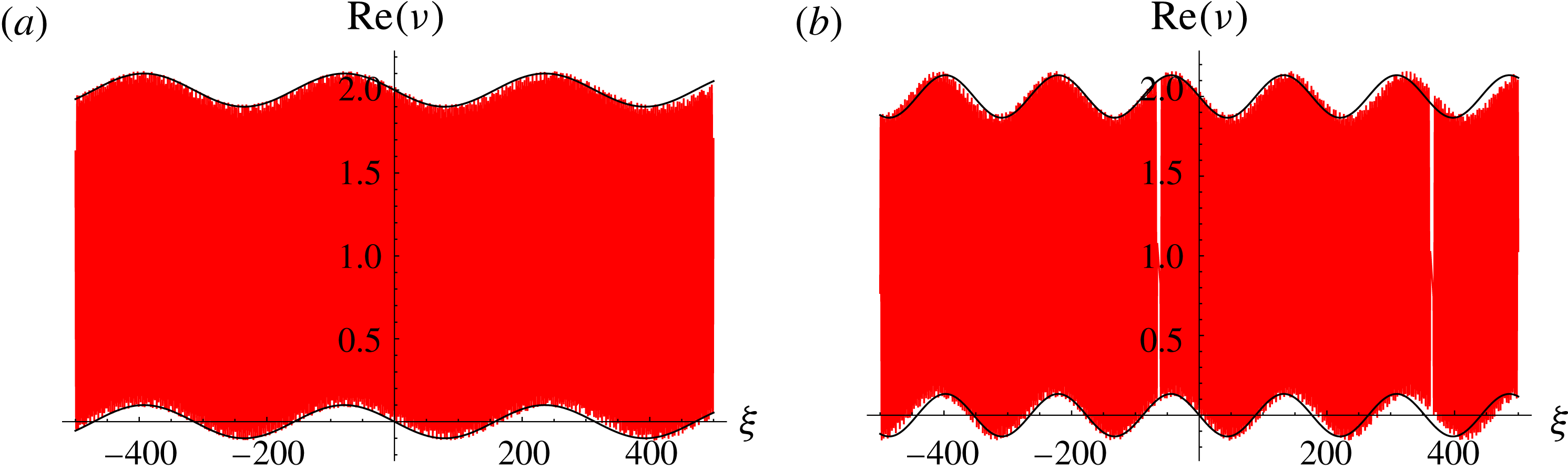
We compare (2.24) and (2.23) with the numerical solution of (2.18) and (2.20) for the same parameters and initial conditions on
 $\unicode[STIX]{x1D707}(\unicode[STIX]{x1D709})$
and
 $\unicode[STIX]{x1D708}(\unicode[STIX]{x1D709})$
as previously but with
 $d=\{10,7.5\}$
in figures 8(a) and 8(b) respectively. In particular, the constants are
 $c_{13}=-\unicode[STIX]{x03C0}/2$
and all other
 $c_{n}=0$
. It should be noted that as
 $\unicode[STIX]{x1D709}\rightarrow \infty$
, the monotonically increasing term in
 $\unicode[STIX]{x1D709}$
dominates in (2.24). Furthermore, we have vertically offset the slowly varying solution to show its fit to the slowly varying envelope. We observe very good quantitative agreement for
 $d=10$
; however, breakdown is apparent when
 $d=7.5$
for
 $\unicode[STIX]{x1D709}\approx 200$
.


2.2.2 Self-similar solutions
We proceed in the same manner as § 2.1.2 by considering a distance function
 $D(t)=d\sqrt{t}$
and self-similar solutions of the form
 $\unicode[STIX]{x1D707}=\sqrt{t}\unicode[STIX]{x1D712}(\unicode[STIX]{x1D702})$
, with the addition of
 $\unicode[STIX]{x1D708}=\sqrt{t}\unicode[STIX]{x1D70C}(\unicode[STIX]{x1D702})$
, for
 $\unicode[STIX]{x1D702}=s/\sqrt{t}$
. Transformation of (2.15) and (2.16) gives
 $$\begin{eqnarray}\displaystyle & \displaystyle {\displaystyle \frac{\text{i}}{2}}\left(\unicode[STIX]{x1D70C}-\unicode[STIX]{x1D702}{\displaystyle \frac{\text{d}\unicode[STIX]{x1D70C}}{\text{d}\unicode[STIX]{x1D702}}}\right)-{\displaystyle \frac{\text{d}^{2}\unicode[STIX]{x1D712}}{\text{d}\unicode[STIX]{x1D702}^{2}}}+4{\displaystyle \frac{\unicode[STIX]{x1D712}+d}{|\unicode[STIX]{x1D712}+d|^{2}}}=0, & \displaystyle\end{eqnarray}$$
 $$\begin{eqnarray}\displaystyle & \displaystyle {\displaystyle \frac{\text{i}}{2}}\left(\unicode[STIX]{x1D712}-\unicode[STIX]{x1D702}{\displaystyle \frac{\text{d}\unicode[STIX]{x1D712}}{\text{d}\unicode[STIX]{x1D702}}}\right)-{\displaystyle \frac{\text{d}^{2}\unicode[STIX]{x1D70C}}{\text{d}\unicode[STIX]{x1D702}^{2}}}=0, & \displaystyle\end{eqnarray}$$
which can be combined by differentiating (2.25) once with respect to
 $\unicode[STIX]{x1D702}$
and substituting (2.26) into this result to obtain
 $$\begin{eqnarray}{\displaystyle \frac{\text{d}^{3}\unicode[STIX]{x1D712}}{\text{d}\unicode[STIX]{x1D702}^{3}}}+{\displaystyle \frac{\unicode[STIX]{x1D702}^{2}}{4}}{\displaystyle \frac{\text{d}\unicode[STIX]{x1D712}}{\text{d}\unicode[STIX]{x1D702}}}-{\displaystyle \frac{\unicode[STIX]{x1D702}}{4}}\unicode[STIX]{x1D712}-4{\displaystyle \frac{\text{d}}{\text{d}\unicode[STIX]{x1D702}}}\left({\displaystyle \frac{\unicode[STIX]{x1D712}+d}{|\unicode[STIX]{x1D712}+d|^{2}}}\right)=0,\end{eqnarray}$$
where the additional initial condition on
 $\unicode[STIX]{x1D712}^{\prime \prime }(\unicode[STIX]{x1D702})$
is calculated by the conditions imposed on
 $\unicode[STIX]{x1D712}(\unicode[STIX]{x1D702})$
,
 $\unicode[STIX]{x1D712}^{\prime }(\unicode[STIX]{x1D702})$
and
 $\unicode[STIX]{x1D70C}^{\prime }(\unicode[STIX]{x1D702})$
in (2.25).
We expand the nonlinear interaction term in (2.27) and use the standard perturbation expansion for
 $\unicode[STIX]{x1D712}(\unicode[STIX]{x1D702})=\sum _{q=0}^{\infty }d^{-q}\unicode[STIX]{x1D712}^{(q)}$
to find
 $$\begin{eqnarray}{\displaystyle \frac{\text{d}^{3}\unicode[STIX]{x1D712}^{(0)}}{\text{d}\unicode[STIX]{x1D702}^{3}}}+{\displaystyle \frac{\unicode[STIX]{x1D702}^{2}}{4}}{\displaystyle \frac{\text{d}\unicode[STIX]{x1D712}^{(0)}}{\text{d}\unicode[STIX]{x1D702}}}-{\displaystyle \frac{\unicode[STIX]{x1D702}}{4}}{\displaystyle \frac{\text{d}\unicode[STIX]{x1D712}^{(0)}}{\text{d}\unicode[STIX]{x1D702}}}+O\left({\displaystyle \frac{1}{d^{2}}}\right)=0,\end{eqnarray}$$
which gives the first-order solution
 $$\begin{eqnarray}\displaystyle \unicode[STIX]{x1D707}(t,s) & = & \displaystyle sc_{1}-c_{2}\left[\sqrt{t}\exp \left(-{\displaystyle \frac{\text{i}s^{2}}{4t}}\right)+{\displaystyle \frac{(-1)^{1/4}\sqrt{\unicode[STIX]{x03C0}}}{2}}s\text{erf}\left({\displaystyle \frac{(-1)^{1/4}s}{2\sqrt{t}}}\right)\right]\nonumber\\ \displaystyle & & \displaystyle +\,c_{3}\left[\text{i}\sqrt{t}\exp \left({\displaystyle \frac{\text{i}s^{2}}{4t}}\right)-{\displaystyle \frac{(-1)^{1/4}\sqrt{\unicode[STIX]{x03C0}}}{2}}s\text{erf}\left({\displaystyle \frac{(-1)^{3/4}s}{2\sqrt{t}}}\right)\right]+O\left({\displaystyle \frac{1}{d^{2}}}\right).\qquad\end{eqnarray}$$
The absence of the
 $O(d^{-1})$
vortex interaction term results in no repulsion of the vortex pair, as seen for the co-rotating pair. The interaction between the pair is
 $O(d^{-2})$
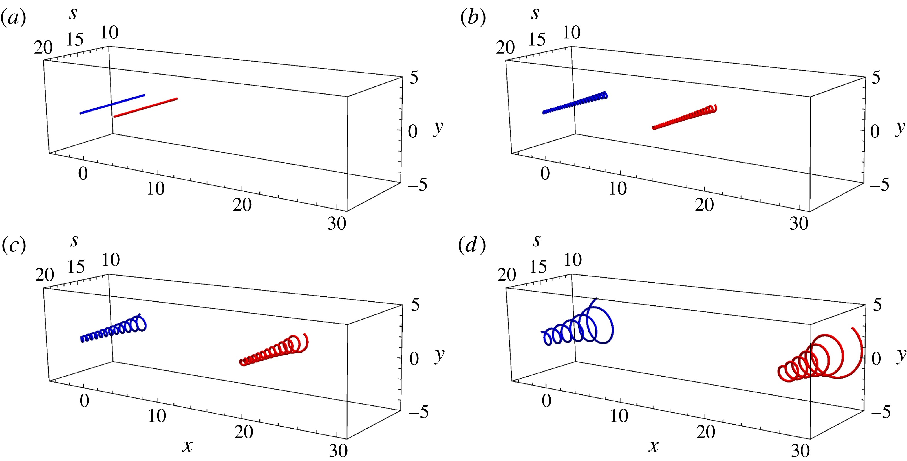
, so that the shape of the filaments in (2.29) is wholly determined by self-induction. The corresponding shape is similar to the co-rotating case in (2.12); that is, the vortices form conical spirals of increasing amplitude and wavelength. We show the vortex filament shapes obtained by numerically solving (2.25) and (2.26) for boundary conditions on
 $\unicode[STIX]{x1D707}(t,s)$
satisfying (2.13) and (2.14) with
 $\unicode[STIX]{x1D70C}(\unicode[STIX]{x1D702}=100)=\unicode[STIX]{x1D70C}^{\prime }(\unicode[STIX]{x1D702}=100)=0$
and
 $d=20$
in figure 9 for times
 $t=\{0.05,0.5,1,2\}$
. We observe that, as with the co-rotating case, the helices rotate in the opposite direction to the respective circulation of the vortex, with
 $\unicode[STIX]{x1D713}_{1}(t,s)$
and
 $\unicode[STIX]{x1D713}_{2}(t,s)$
having circulations
 $\unicode[STIX]{x1D6E4}_{1}>0$
and
 $\unicode[STIX]{x1D6E4}_{2}<0$
. The helices are now reflections of each other across the
 $y$
-axis.
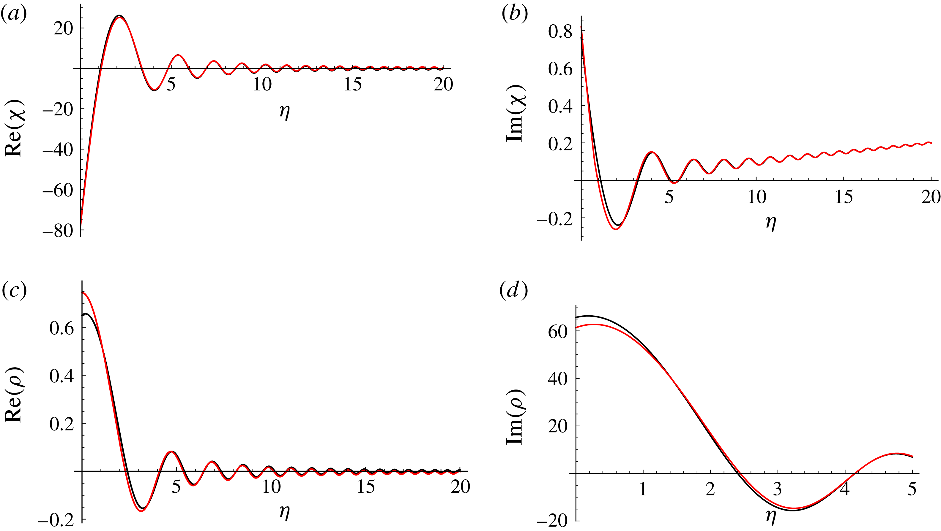
We compare the real and imaginary components of the asymptotic solution (2.29) with the numerical solutions for the same conditions in figure 10. In this case, the boundary condition necessary to determine the third condition on
 $\unicode[STIX]{x1D712}(\unicode[STIX]{x1D702})$
is
 $\unicode[STIX]{x1D712}^{\prime \prime }(\unicode[STIX]{x1D702}=100)=4d^{-1}(1+d^{-1}(1-\text{i}))^{-1}$
by (2.25). Expansion of the condition for
 $d^{-1}\ll 1$
gives
 $\unicode[STIX]{x1D712}^{\prime \prime }(\unicode[STIX]{x1D702}=100)=O(d^{-2})$
, which we impose to find the zeroth-order solution
 $\unicode[STIX]{x1D712}^{(0)}(\unicode[STIX]{x1D702})$
and subsequently find the corresponding
 $\unicode[STIX]{x1D70C}^{(0)}(\unicode[STIX]{x1D702})$
from (2.26). We note that the asymptotic solution shows good agreement with the numerical solutions, but breaks down as longer time scales are considered.
The time evolution of self-similarity solutions in counter-rotating vortices held apart by a distance function
 $D(t)=d\sqrt{t}$
, with
 $\unicode[STIX]{x1D713}_{1}(t,s)$
and
 $\unicode[STIX]{x1D713}_{2}(t,s)$
being denoted by blue and red respectively. In particular, numerical solutions of (2.25) and (2.26), with conditions satisfying (2.13), (2.14), and
 $\unicode[STIX]{x1D70C}(\unicode[STIX]{x1D702}=100)=\unicode[STIX]{x1D70C}^{\prime }(\unicode[STIX]{x1D702}=100)=0$
, have been plotted for
 $d=20$
over
 $s\in [10,20]$
. The times shown are (a)
 $t=0.05$
, (b)
 $t=0.5$
, (c)
 $t=1$
and (d)
 $t=2$
.
3 Intertwining vortex pairs
We now consider the case where the distance function
 $D(t)$
vanishes. The vortices now intertwine and revolve around each other, with
 $\unicode[STIX]{x1D708}(t,s)$
describing the centre of revolution and
 $\unicode[STIX]{x1D707}(t,s)$
coinciding with the deviations from this centre (see figure 11). The equations describing the time evolution of the vortex pair are now given by
 $$\begin{eqnarray}\displaystyle & \displaystyle \text{i}{\displaystyle \frac{\unicode[STIX]{x2202}\unicode[STIX]{x1D708}}{\unicode[STIX]{x2202}t}}+{\displaystyle \frac{1}{2}}(1+\unicode[STIX]{x1D6F1}){\displaystyle \frac{\unicode[STIX]{x2202}^{2}\unicode[STIX]{x1D708}}{\unicode[STIX]{x2202}s^{2}}}-{\displaystyle \frac{1}{2}}(1-\unicode[STIX]{x1D6F1}){\displaystyle \frac{\unicode[STIX]{x2202}^{2}\unicode[STIX]{x1D707}}{\unicode[STIX]{x2202}s^{2}}}+2(1-\unicode[STIX]{x1D6F1}){\displaystyle \frac{\unicode[STIX]{x1D707}}{|\unicode[STIX]{x1D707}|^{2}}}=0, & \displaystyle\end{eqnarray}$$
 $$\begin{eqnarray}\displaystyle & \displaystyle \text{i}{\displaystyle \frac{\unicode[STIX]{x2202}\unicode[STIX]{x1D707}}{\unicode[STIX]{x2202}t}}-{\displaystyle \frac{1}{2}}(1-\unicode[STIX]{x1D6F1}){\displaystyle \frac{\unicode[STIX]{x2202}^{2}\unicode[STIX]{x1D708}}{\unicode[STIX]{x2202}s^{2}}}+{\displaystyle \frac{1}{2}}(1+\unicode[STIX]{x1D6F1}){\displaystyle \frac{\unicode[STIX]{x2202}^{2}\unicode[STIX]{x1D707}}{\unicode[STIX]{x2202}s^{2}}}+2(1+\unicode[STIX]{x1D6F1}){\displaystyle \frac{\unicode[STIX]{x1D707}}{|\unicode[STIX]{x1D707}|^{2}}}=0. & \displaystyle\end{eqnarray}$$
Real and imaginary components of
 $\unicode[STIX]{x1D712}(\unicode[STIX]{x1D702})$
and
 $\unicode[STIX]{x1D70C}(\unicode[STIX]{x1D702})$
obtained by the asymptotic solution (2.26) and (2.29) (shown in black) and the numerical solution of (2.25) and (2.26) (shown in red). The initial conditions are
 $\unicode[STIX]{x1D712}(\unicode[STIX]{x1D702}=100)=1+\text{i}$
,
 $\unicode[STIX]{x1D712}^{\prime }(\unicode[STIX]{x1D702}=100)=1$
,
 $\unicode[STIX]{x1D70C}(\unicode[STIX]{x1D702}=100)=0$
and
 $\unicode[STIX]{x1D70C}^{\prime }(\unicode[STIX]{x1D702}=100)=0$
, with
 $d=20$
.
Intertwining vortex coordinates
 $\unicode[STIX]{x1D707}(t,s)$
and
 $\unicode[STIX]{x1D708}(t,s)$
and how they relate to filaments
 $\unicode[STIX]{x1D713}_{1}(t,s)$
and
 $\unicode[STIX]{x1D713}_{2}(t,s)$
in the case of no separation function (i.e.
 $D(t)=0$
).
3.1 Co-rotating vortices
We again study pairs whose vortices have the same circulation
 $\unicode[STIX]{x1D6F1}=1$
. Equations (3.1) and (3.2) decouple in a similar manner to that in § 2.1,
 $$\begin{eqnarray}\displaystyle & \displaystyle \text{i}{\displaystyle \frac{\unicode[STIX]{x2202}\unicode[STIX]{x1D708}}{\unicode[STIX]{x2202}t}}+{\displaystyle \frac{\unicode[STIX]{x2202}^{2}\unicode[STIX]{x1D708}}{\unicode[STIX]{x2202}s^{2}}}=0, & \displaystyle\end{eqnarray}$$
 $$\begin{eqnarray}\displaystyle & \displaystyle \text{i}{\displaystyle \frac{\unicode[STIX]{x2202}\unicode[STIX]{x1D707}}{\unicode[STIX]{x2202}t}}+{\displaystyle \frac{\unicode[STIX]{x2202}^{2}\unicode[STIX]{x1D707}}{\unicode[STIX]{x2202}s^{2}}}+{\displaystyle \frac{4\unicode[STIX]{x1D707}}{|\unicode[STIX]{x1D707}|^{2}}}=0, & \displaystyle\end{eqnarray}$$
so that, for the following analysis, we will only consider the nonlinear Schrödinger-type equation given by (3.4).
We suppose that
 $\unicode[STIX]{x1D707}(t,s)$
has an amplitude and phase ansatz given by
 $$\begin{eqnarray}\unicode[STIX]{x1D707}(t,s)=A(t,s)\text{exp}(\text{i}\unicode[STIX]{x1D703}(t,s)),\end{eqnarray}$$
with
 $A(t,s)\in \mathbb{R}$
measuring the separation of the vortex pair and
 $\unicode[STIX]{x1D703}(t,s)\in \mathbb{R}$
measuring the orientation of separation from the positive
 $x$
-axis.
Upon separating (3.4) into real and imaginary components using (3.5), we find
 $$\begin{eqnarray}\displaystyle & \displaystyle -A{\displaystyle \frac{\unicode[STIX]{x2202}\unicode[STIX]{x1D703}}{\unicode[STIX]{x2202}t}}+{\displaystyle \frac{\unicode[STIX]{x2202}^{2}A}{\unicode[STIX]{x2202}s^{2}}}-A\left({\displaystyle \frac{\unicode[STIX]{x2202}\unicode[STIX]{x1D703}}{\unicode[STIX]{x2202}s}}\right)^{2}+{\displaystyle \frac{4}{A}}=0, & \displaystyle\end{eqnarray}$$
 $$\begin{eqnarray}\displaystyle & \displaystyle {\displaystyle \frac{\unicode[STIX]{x2202}A}{\unicode[STIX]{x2202}t}}+A{\displaystyle \frac{\unicode[STIX]{x2202}^{2}\unicode[STIX]{x1D703}}{\unicode[STIX]{x2202}s^{2}}}+2{\displaystyle \frac{\unicode[STIX]{x2202}A}{\unicode[STIX]{x2202}s}}{\displaystyle \frac{\unicode[STIX]{x2202}\unicode[STIX]{x1D703}}{\unicode[STIX]{x2202}s}}=0. & \displaystyle\end{eqnarray}$$
By multiplying (3.7) by
 $A(t,s)$
, we note that it can be written as a conservation law
 $$\begin{eqnarray}{\displaystyle \frac{1}{2}}{\displaystyle \frac{\unicode[STIX]{x2202}}{\unicode[STIX]{x2202}t}}(A^{2})+{\displaystyle \frac{\unicode[STIX]{x2202}}{\unicode[STIX]{x2202}s}}\left(A^{2}{\displaystyle \frac{\unicode[STIX]{x2202}\unicode[STIX]{x1D703}}{\unicode[STIX]{x2202}s}}\right)=0,\end{eqnarray}$$
which is a statement on the evolution of the vortex pair separation squared,
 $A^{2}$
, and how it is connected to the gradient of that same separation together with the pair twist,
 $\unicode[STIX]{x2202}\unicode[STIX]{x1D703}/\unicode[STIX]{x2202}s$
, along the filament arclength
 $s$
. For vortices that are straight under some orientation,
 $\unicode[STIX]{x2202}\unicode[STIX]{x1D703}/\unicode[STIX]{x2202}s=0$
and the separation between vortices at a particular
 $s$
will not change for all time. However, if the pair are highly coiled, such that
 $\unicode[STIX]{x2202}\unicode[STIX]{x1D703}/\unicode[STIX]{x2202}s\rightarrow \infty$
, then slight deviations in
 $A(t,s)$
along the filaments will result in very rapid changes in the pair separation.
3.1.1 Plane-wave solutions
We consider rotating helix solutions to (3.4) of the form
 $$\begin{eqnarray}\unicode[STIX]{x1D707}(t,s)=A_{0}\exp (\text{i}(ks-\unicode[STIX]{x1D714}t)),\end{eqnarray}$$
where
 $A_{0}$
is the constant amplitude of separation,
 $k$
is the wavenumber related to the twist of the helix,
 $\unicode[STIX]{x1D714}$
is the rotational velocity and
 $A_{0},k,\unicode[STIX]{x1D714}\in \mathbb{R}$
.
Substitution of (3.9) into (3.4) gives the dispersion relation
 $$\begin{eqnarray}\unicode[STIX]{x1D714}=k^{2}-{\displaystyle \frac{4}{A_{0}}},\end{eqnarray}$$
a result that has previously been found by Klein et al. (Reference Klein, Majda and Damodaran1995). However, (3.10) implies that the vortex pair can rotate clockwise, anticlockwise or not at all depending on the twist of the helical solution and its amplitude, regardless of the individual circulation of the vortices.
3.1.2 Travelling wave solutions
We introduce the same wave coordinate
 $\unicode[STIX]{x1D709}=s-vt$
seen in the aforementioned analysis, for
 $v$
a constant. Transforming relations (3.6) and (3.8), we find
 $$\begin{eqnarray}\displaystyle & \displaystyle {\displaystyle \frac{\text{d}^{2}A}{\text{d}\unicode[STIX]{x1D709}^{2}}}+vA{\displaystyle \frac{\text{d}\unicode[STIX]{x1D703}}{\text{d}\unicode[STIX]{x1D709}}}-A\left({\displaystyle \frac{\text{d}\unicode[STIX]{x1D703}}{\text{d}\unicode[STIX]{x1D709}}}\right)^{2}+{\displaystyle \frac{4}{A}}=0, & \displaystyle\end{eqnarray}$$
 $$\begin{eqnarray}\displaystyle & \displaystyle {\displaystyle \frac{\text{d}}{\text{d}\unicode[STIX]{x1D709}}}\left(A^{2}{\displaystyle \frac{\text{d}\unicode[STIX]{x1D703}}{\text{d}\unicode[STIX]{x1D709}}}\right)-{\displaystyle \frac{v}{2}}{\displaystyle \frac{\text{d}}{\text{d}\unicode[STIX]{x1D709}}}(A^{2})=0. & \displaystyle\end{eqnarray}$$
Solutions to these equations will effectively generalise the plane-wave or helix solutions of Klein et al. (Reference Klein, Majda and Damodaran1995) mentioned above, as those solutions correspond to the case where
 $A$
is constant.
We note that (3.11) and (3.12) allow the exact implicit solution
 $$\begin{eqnarray}\unicode[STIX]{x1D709}-\unicode[STIX]{x1D709}_{0}=\pm \int {\displaystyle \frac{\text{d}A}{\sqrt{2(E-V(A))}}},\end{eqnarray}$$
where
 $\unicode[STIX]{x1D709}_{0},E\in \mathbb{R}$
are integration constants and
 $V(A)$
is a Hamiltonian potential given by
 $$\begin{eqnarray}V(A)={\displaystyle \frac{v^{2}}{8}}A^{2}+4\ln A+{\displaystyle \frac{\unicode[STIX]{x1D6FE}^{2}}{2A^{2}}},\end{eqnarray}$$
where
 $\unicode[STIX]{x1D6FE}\in \mathbb{R}$
is another integration constant that is a measure of coupling between the vortex pair separation and changes in its orientation (see § B.1).
We comment on some important aspects of (3.14). The potential function implies that all travelling wave solutions will be attracted to
 $A\rightarrow 0^{+}$
as
 $\unicode[STIX]{x1D709}\rightarrow \pm \infty$
if
 $\unicode[STIX]{x1D6FE}=0$
, resulting in collapse of the vortex pair as
 $t\rightarrow \pm \infty$
. Coupling between the amplitude of separation and the angular velocity of the pair is necessary to sustain travelling wave solutions for co-rotating pairs. When
 $\unicode[STIX]{x1D6FE}\neq 0$
, (3.8) predicts that
 $A$
will have periodic trajectories such that
 $A>0$
for all time. However, for
 $\unicode[STIX]{x1D6FE}\ll 1$
, there are three different asymptotic regimes in (3.11) and (3.12) (for full details of the other regimes, see § B.1), the most noteworthy of which is
 $A(\unicode[STIX]{x1D709})=O(\unicode[STIX]{x1D6FE}^{n})$
for
 $n>1$
. In this case, there exists an initial layer of width
 $\unicode[STIX]{x1D6FE}^{2n-1}$
so that
 $A^{\prime \prime }\sim 1/A^{3}$
and the leading-order behaviour is
 $$\begin{eqnarray}\displaystyle & \displaystyle A\left({\displaystyle \frac{\unicode[STIX]{x1D709}}{\unicode[STIX]{x1D6FE}^{2n-1}}}\right)\sim {\displaystyle \frac{\pm 1}{\sqrt{c_{1}}}}\sqrt{1+c_{1}^{2}c_{2}^{2}+2c_{1}^{2}c_{2}{\displaystyle \frac{\unicode[STIX]{x1D709}}{\unicode[STIX]{x1D6FE}^{2n-1}}}+c_{1}^{2}{\displaystyle \frac{\unicode[STIX]{x1D709}^{2}}{\unicode[STIX]{x1D6FE}^{4n-2}}}}, & \displaystyle\end{eqnarray}$$
 $$\begin{eqnarray}\displaystyle & \displaystyle \unicode[STIX]{x1D703}\left({\displaystyle \frac{\unicode[STIX]{x1D709}}{\unicode[STIX]{x1D6FE}^{2n-1}}}\right)\sim \unicode[STIX]{x1D6FE}\tan ^{-1}\left({\displaystyle \frac{\unicode[STIX]{x1D709}}{\unicode[STIX]{x1D6FE}^{2n-1}}}c_{1}+c_{1}c_{2}\right)+{\displaystyle \frac{v}{2}}{\displaystyle \frac{\unicode[STIX]{x1D709}}{\unicode[STIX]{x1D6FE}^{2n-1}}}+\unicode[STIX]{x1D703}_{0}, & \displaystyle\end{eqnarray}$$
for
 $c_{1},c_{2},\unicode[STIX]{x1D703}_{0}\in \mathbb{R}$
.
We illustrate the vortex pair by numerically solving (3.11) and (3.12) and compare these results with those from the leading-order behaviour and the implicit solution (3.13). In particular, we consider the conditions
 $A(\unicode[STIX]{x1D709}=0)=1$
,
 $A^{\prime }(\unicode[STIX]{x1D709}=0)=0$
and
 $\unicode[STIX]{x1D703}(\unicode[STIX]{x1D709}=0)=0$
, with
 $\unicode[STIX]{x1D6FE}=0.001$
and
 $v=1$
. For these parameters, the trajectories of
 $A$
are such that they never exceed the potential given by
 $v^{2}/8+\unicode[STIX]{x1D6FE}^{2}/2$
, according to (3.14), constraining the values of
 $A$
to the range
 $A\in [1.17\times 10^{-5},1]$
, and, furthermore, the period of oscillation in
 $A(\unicode[STIX]{x1D709})$
is
 $T\approx 1.226$
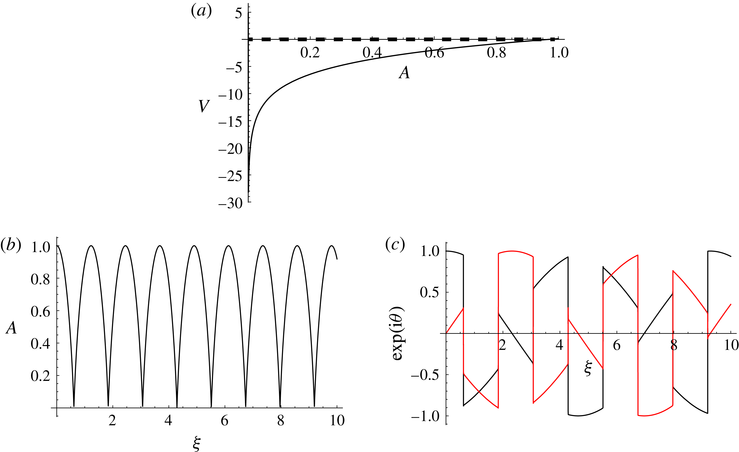
by solving (3.13). We plot the potential (3.14), corresponding
 $A(\unicode[STIX]{x1D709})$
, and the real and imaginary components of
 $\text{exp}(\text{i}\unicode[STIX]{x1D703}(\unicode[STIX]{x1D709}))$
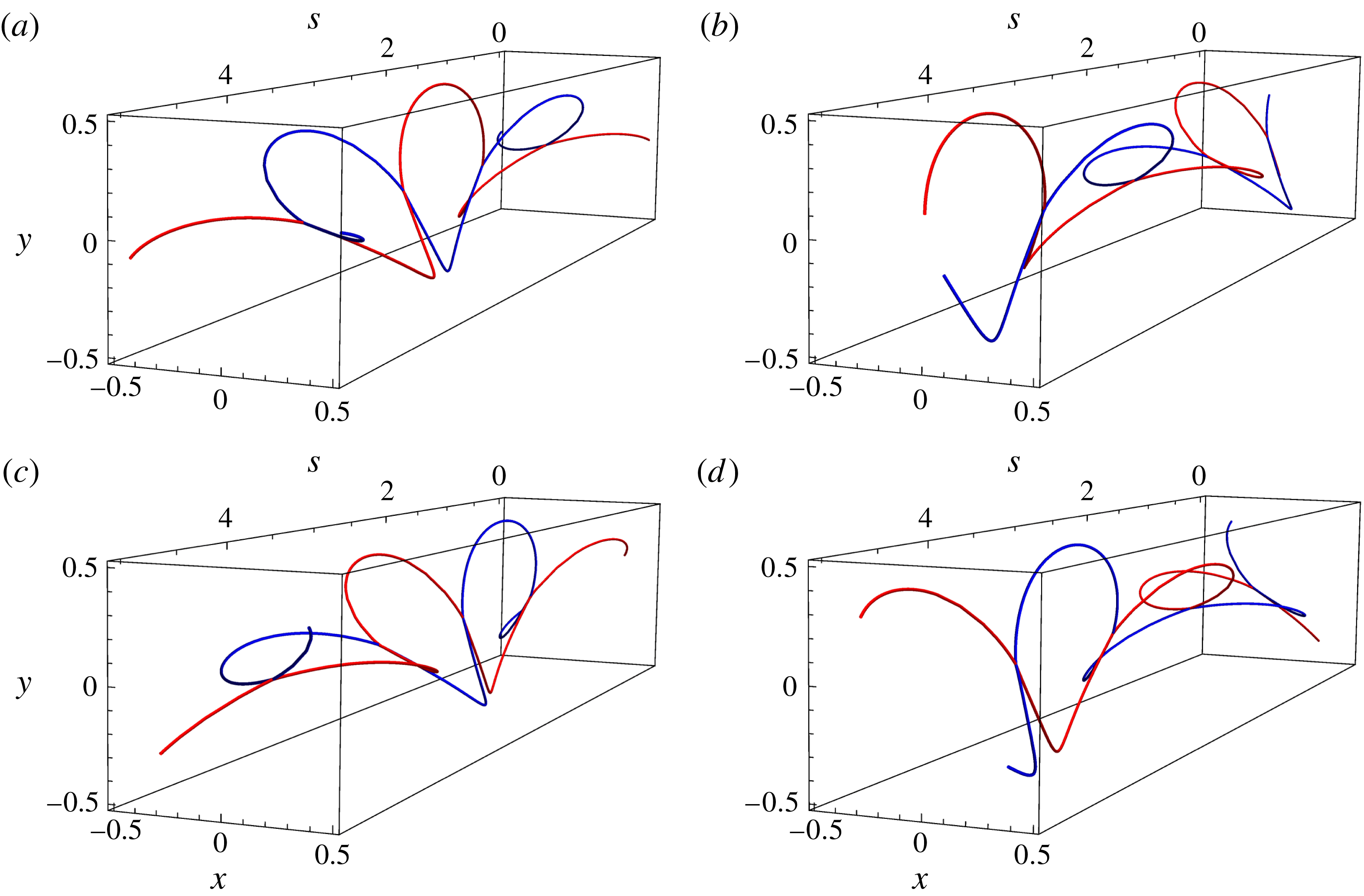
in figures 12(a), 12(b) and 12(c) respectively as well as the shape of the vortex pair at
 $t=\{0,2,4,6\}$
with
 $\unicode[STIX]{x1D708}(t,s)=0$
(shown in figure 13(a–d)).
From figure 12(b), we observe that the period of oscillation is indeed
 $T\approx 1.226$
, and furthermore note that the numerical solutions show similarities to (3.15) for small
 $A(\unicode[STIX]{x1D709})$
; in particular, the sharp cusp that was predicted in the regime
 $A=O(\unicode[STIX]{x1D6FE}^{n})$
for
 $n>1$
. As the vortices approach each other, their attraction occurs on a very fast time scale, for
 $\unicode[STIX]{x1D6FE}\ll 1$
, until the pair reaches their minimum separation whereby they repel. The orientation of the vortices at this moment changes almost instantaneously, as
 $\unicode[STIX]{x1D6FE}\tan ^{-1}(c_{1}c_{2}+c_{1}\unicode[STIX]{x1D709}/\unicode[STIX]{x1D6FE}^{2n-1})$
dominates in (3.16). As the vortices repel and
 $A\rightarrow O(1)$
, the time scale slows down and the orientation of the pair evolves according to the
 $v\unicode[STIX]{x1D709}/2$
term, which now plays a role in (B 6). The vortices reach their maximum separation before attracting each other again and repeating the cycle.
(a) Potential of the separation equation as defined in (3.14), and numerical solutions of (b)
 $A(\unicode[STIX]{x1D709})$
and (c) the real and imaginary parts of the complex exponential
 $\text{exp}(\text{i}\unicode[STIX]{x1D703}(\unicode[STIX]{x1D709}))$
(shown in black and red respectively). The numerical solutions were obtained by solving (B 1) and (B 2) for
 $v=1$
and
 $\unicode[STIX]{x1D6FE}=0.001$
, with initial conditions
 $A(\unicode[STIX]{x1D709}=0)=1$
,
 $A^{\prime }(\unicode[STIX]{x1D709}=0)=0$
and
 $\unicode[STIX]{x1D703}(\unicode[STIX]{x1D709}=0)=0$
. The trajectories of
 $A(\unicode[STIX]{x1D709})$
are restricted in the potential well such that they never exceed the potential
 $v^{2}/8+\unicode[STIX]{x1D6FE}^{2}/2$
, shown by the dashed line, and oscillate with period
 $T\approx 1.226$
, by (3.13).
Time evolution of travelling wave solutions in intertwining co-rotating vortices, with
 $\unicode[STIX]{x1D713}_{1}(t,s)$
and
 $\unicode[STIX]{x1D713}_{2}(t,s)$
shown in blue and red respectively. Numerical solutions of (B 1) and (B 2), with
 $\unicode[STIX]{x1D708}(\unicode[STIX]{x1D709})=0$
, are plotted over
 $s\in [0,5]$
. In particular, the initial conditions are
 $A(\unicode[STIX]{x1D709}=0)=1$
,
 $A^{\prime }(\unicode[STIX]{x1D709}=0)=0$
and
 $\unicode[STIX]{x1D703}(\unicode[STIX]{x1D709}=0)=0$
, with parameters
 $v=1$
and
 $\unicode[STIX]{x1D6FE}=0.001$
. The times shown are (a)
 $t=0$
, (b)
 $t=2$
, (c)
 $t=4$
and (d)
 $t=8$
.
3.1.3 Purely rotating-wave solutions
We study solutions of the rotating-wave ansatz
 $$\begin{eqnarray}\displaystyle & \displaystyle A(t,s)=A(s), & \displaystyle\end{eqnarray}$$
 $$\begin{eqnarray}\displaystyle & \displaystyle \unicode[STIX]{x1D703}(t,s)=-\unicode[STIX]{x1D714}t, & \displaystyle\end{eqnarray}$$
where
 $\unicode[STIX]{x1D714}$
is the constant angular velocity of the rotating wave. The resulting solutions are each effectively planar filaments, as they maintain their spatial structure while the only motion is pure rotation; see Van Gorder (Reference Van Gorder2015b
) and references therein.
Substitution of this ansatz into (3.6) gives
 $$\begin{eqnarray}{\displaystyle \frac{\text{d}^{2}A}{\text{d}s^{2}}}+\unicode[STIX]{x1D714}A+{\displaystyle \frac{4}{A}}=0,\end{eqnarray}$$
which, following the treatment of § B.1, has the exact implicit solution
 $$\begin{eqnarray}\displaystyle s-s_{0}=\int {\displaystyle \frac{\text{d}A}{\sqrt{2(E-V(A))}}}, & & \displaystyle\end{eqnarray}$$
where
 $s_{0},E\in \mathbb{R}$
are integration constants and the Hamiltonian potential is given by
 $$\begin{eqnarray}V(A)={\displaystyle \frac{\unicode[STIX]{x1D714}A^{2}}{2}}+4\ln A.\end{eqnarray}$$
We note that (3.21) is not bounded from below, suggesting that, for all rotating-wave solutions with
 $\unicode[STIX]{x1D714}>0$
,
 $A\rightarrow 0^{+}$
as
 $s\rightarrow \pm \infty$
; the vortex pair will collapse if their respective circulations are in the same direction as the pair rotates in. If
 $\unicode[STIX]{x1D714}<0$
, then another possibility arises, namely
 $A\rightarrow \infty$
as
 $s\rightarrow \infty$
, as the potential is not bound from above. If we consider a vortex pair with circulations in the opposite direction, then rotating pairs with
 $\unicode[STIX]{x1D714}<0$
will collapse or, if
 $\unicode[STIX]{x1D714}>0$
, may also repel without bound.
To illustrate the aforementioned description of the vortex shapes, we plot the numerical solution of (3.19) with
 $\unicode[STIX]{x1D708}(t,s)=0$
for the case of
 $\unicode[STIX]{x1D714}>0$
and
 $\unicode[STIX]{x1D714}<0$
. In particular, we consider
 $\unicode[STIX]{x1D714}=1$
for the initial conditions
 $A(s=0)=1$
and
 $A(s=0)=5$
(shown in figure 14
a,b), and
 $\unicode[STIX]{x1D714}=-1$
for conditions
 $A(s=0)=1$
and
 $A(s=0)=1.8$
, both at times
 $t=\{0,2\}$
. We note that, as predicted, the solutions for
 $\unicode[STIX]{x1D714}>0$
exhibit eventual collapse of the pair for increasing
 $s$
, while solutions for
 $\unicode[STIX]{x1D714}<0$
show unbounded growth of the pair for increasing
 $s$
.
Time evolution of planar rotating filament solutions in intertwining co-rotating vortices, with
 $\unicode[STIX]{x1D713}_{1}(t,s)$
and
 $\unicode[STIX]{x1D713}_{2}(t,s)$
shown in blue and red respectively. Numerical solutions of (3.19), with
 $\unicode[STIX]{x1D708}(t,s)=0$
, are plotted over
 $s\in [0,9]$
. In particular, the initial conditions and parameters are
 $A(\unicode[STIX]{x1D709}=0)=1$
,
 $A^{\prime }(\unicode[STIX]{x1D709}=0)=5$
and
 $\unicode[STIX]{x1D714}=1$
(a,b), and
 $A(\unicode[STIX]{x1D709}=0)=1$
,
 $A^{\prime }(\unicode[STIX]{x1D709}=0)=1.8$
and
 $\unicode[STIX]{x1D714}=-1$
(c,d), both of which are plotted at times
 $t=\{0,2\}$
.
3.1.4 Self-similar solutions
We transform (3.4) into the variables
 $\unicode[STIX]{x1D707}(t,s)=s\unicode[STIX]{x1D712}(\unicode[STIX]{x1D702})$
, with
 $\unicode[STIX]{x1D702}=s/\sqrt{t}$
,
 $$\begin{eqnarray}\unicode[STIX]{x1D702}^{2}{\displaystyle \frac{\text{d}^{2}\unicode[STIX]{x1D712}}{\text{d}\unicode[STIX]{x1D702}^{2}}}+\left(2\unicode[STIX]{x1D702}-{\displaystyle \frac{\text{i}\unicode[STIX]{x1D702}^{3}}{2}}\right){\displaystyle \frac{\text{d}\unicode[STIX]{x1D712}}{\text{d}\unicode[STIX]{x1D702}}}+{\displaystyle \frac{4\unicode[STIX]{x1D712}}{|\unicode[STIX]{x1D712}|^{2}}}=0,\end{eqnarray}$$
and use the amplitude–phase ansatz for
 $\unicode[STIX]{x1D712}(\unicode[STIX]{x1D702})$
to simplify the vortex interaction term,
 $$\begin{eqnarray}\unicode[STIX]{x1D712}(\unicode[STIX]{x1D702})=A(\unicode[STIX]{x1D702})\text{e}^{\text{i}\unicode[STIX]{x1D703}(\unicode[STIX]{x1D702})},\end{eqnarray}$$
which, substituting into (3.22) and separating real and imaginary components, gives
 $$\begin{eqnarray}\displaystyle & \displaystyle \unicode[STIX]{x1D702}^{2}{\displaystyle \frac{\text{d}^{2}A}{\text{d}\unicode[STIX]{x1D702}^{2}}}-\unicode[STIX]{x1D702}^{2}A\left({\displaystyle \frac{\text{d}\unicode[STIX]{x1D703}}{\text{d}\unicode[STIX]{x1D702}}}\right)^{2}+2\unicode[STIX]{x1D702}{\displaystyle \frac{\text{d}A}{\text{d}\unicode[STIX]{x1D702}}}+{\displaystyle \frac{\unicode[STIX]{x1D702}^{3}}{2}}A{\displaystyle \frac{\text{d}\unicode[STIX]{x1D703}}{\text{d}\unicode[STIX]{x1D702}}}+{\displaystyle \frac{4}{A}}=0, & \displaystyle\end{eqnarray}$$
 $$\begin{eqnarray}\displaystyle & \displaystyle \unicode[STIX]{x1D702}^{2}A{\displaystyle \frac{\text{d}^{2}\unicode[STIX]{x1D703}}{\text{d}\unicode[STIX]{x1D702}^{2}}}+2\unicode[STIX]{x1D702}^{2}{\displaystyle \frac{\text{d}A}{\text{d}\unicode[STIX]{x1D702}}}{\displaystyle \frac{\text{d}\unicode[STIX]{x1D703}}{\text{d}\unicode[STIX]{x1D702}}}+2\unicode[STIX]{x1D702}A{\displaystyle \frac{\text{d}\unicode[STIX]{x1D703}}{\text{d}\unicode[STIX]{x1D702}}}-{\displaystyle \frac{\unicode[STIX]{x1D702}^{3}}{2}}{\displaystyle \frac{\text{d}A}{\text{d}\unicode[STIX]{x1D702}}}=0. & \displaystyle\end{eqnarray}$$
By multiplying (3.25) through by
 $A(\unicode[STIX]{x1D702})$
and dividing by
 $\unicode[STIX]{x1D702}^{2}$
, we obtain
 $$\begin{eqnarray}{\displaystyle \frac{\text{d}}{\text{d}\unicode[STIX]{x1D702}}}\left(A^{2}{\displaystyle \frac{\text{d}\unicode[STIX]{x1D703}}{\text{d}\unicode[STIX]{x1D702}}}\right)+{\displaystyle \frac{2}{\unicode[STIX]{x1D702}}}A^{2}{\displaystyle \frac{\text{d}\unicode[STIX]{x1D703}}{\text{d}\unicode[STIX]{x1D702}}}-{\displaystyle \frac{\unicode[STIX]{x1D702}}{4}}{\displaystyle \frac{\text{d}}{\text{d}\unicode[STIX]{x1D702}}}(A^{2})=0,\end{eqnarray}$$
which is a linear equation in
 $A^{2}\unicode[STIX]{x1D703}^{\prime }(\unicode[STIX]{x1D702})$
that can be integrated to give
 $$\begin{eqnarray}{\displaystyle \frac{\text{d}\unicode[STIX]{x1D703}}{\text{d}\unicode[STIX]{x1D702}}}={\displaystyle \frac{\unicode[STIX]{x1D6FE}}{\unicode[STIX]{x1D702}^{2}A^{2}}}+{\displaystyle \frac{1}{\unicode[STIX]{x1D702}^{2}A^{2}}}\int {\displaystyle \frac{\unicode[STIX]{x1D702}^{3}}{4}}{\displaystyle \frac{\text{d}}{\text{d}\unicode[STIX]{x1D702}}}(A^{2})\,\text{d}\unicode[STIX]{x1D702},\end{eqnarray}$$
where
 $\unicode[STIX]{x1D6FE}\in \mathbb{R}$
is an integration constant. It should be noted that, compared with the travelling wave solutions in § 3.1.2,
 $\unicode[STIX]{x1D6FE}$
does not quantify the degree of coupling between the changing orientation of the vortex separation and the amplitude of separation, because if
 $\unicode[STIX]{x1D6FE}=0$
, there is still dependence of
 $\unicode[STIX]{x1D703}^{\prime }(\unicode[STIX]{x1D702})$
on
 $A(\unicode[STIX]{x1D702})$
.
We numerically solve (3.24) and (3.27) for the boundary conditions
 $A(\unicode[STIX]{x1D702}=0.001)=5$
,
 $A^{\prime }(\unicode[STIX]{x1D702}=0.001)=1$
,
 $\unicode[STIX]{x1D703}(\unicode[STIX]{x1D702}=0.001)=0$
,
 $\unicode[STIX]{x1D703}^{\prime }(\unicode[STIX]{x1D702}=0.001)=0$
, and plot
 $A(\unicode[STIX]{x1D702})$
and
 $\text{exp}(\text{i}\unicode[STIX]{x1D703}(\unicode[STIX]{x1D702}))$
in figures 15(a) and 15(b) respectively, and the corresponding vortex filament shapes in figure 16 for
 $\unicode[STIX]{x1D708}(t,s)=0$
at times
 $t=\{10,50,100,500,1000,5000\}$
.
We observe a number of interesting aspects. First, given the conditions on
 $A(\unicode[STIX]{x1D702})$
and
 $\unicode[STIX]{x1D703}(\unicode[STIX]{x1D702})$
, we note that
 $\unicode[STIX]{x1D6FE}\neq 0$
, which implies that when
 $A(\unicode[STIX]{x1D702})\rightarrow 0^{+}$
, then
 $\unicode[STIX]{x1D703}^{\prime }(\unicode[STIX]{x1D702})\rightarrow \pm \infty$
. In a similar manner to that in § 3.1.2 for the case of
 $\unicode[STIX]{x1D6FE}\neq 0$
, when the vortex pair come into close proximity, the orientation of separation changes rapidly, as we note in figure 15(a,b). Furthermore, as
 $\unicode[STIX]{x1D702}\rightarrow 0^{+}$
, corresponding to time
 $t\rightarrow \infty$
, the amplitude and the wavelength of the vortex separation become larger and the changes in orientation become slower. We note that these results follow directly from the self-similar nature of the vortex pair, which exhibit an initial shape (figure 16
a) that becomes increasingly zoomed in (figure 16
b–f) for increasing times. As
 $t\rightarrow \infty$
, the separation of the vortices themselves will grow to infinity, and their orientation will be planar along a single direction.
Numerical solutions of (a)
 $A(\unicode[STIX]{x1D702})$
and (b) real and imaginary parts of the complex exponential
 $\text{exp}(\text{i}\unicode[STIX]{x1D703}(\unicode[STIX]{x1D702}))$
(shown in black and red respectively), obtained by solving (3.24) and (3.27) with initial conditions
 $A(\unicode[STIX]{x1D702}=0.001)=5$
,
 $A^{\prime }(\unicode[STIX]{x1D702}=0.001)=1$
,
 $\unicode[STIX]{x1D703}(\unicode[STIX]{x1D702}=0.001)=0$
and
 $\unicode[STIX]{x1D703}^{\prime }(\unicode[STIX]{x1D702}=0.001)=0$
.
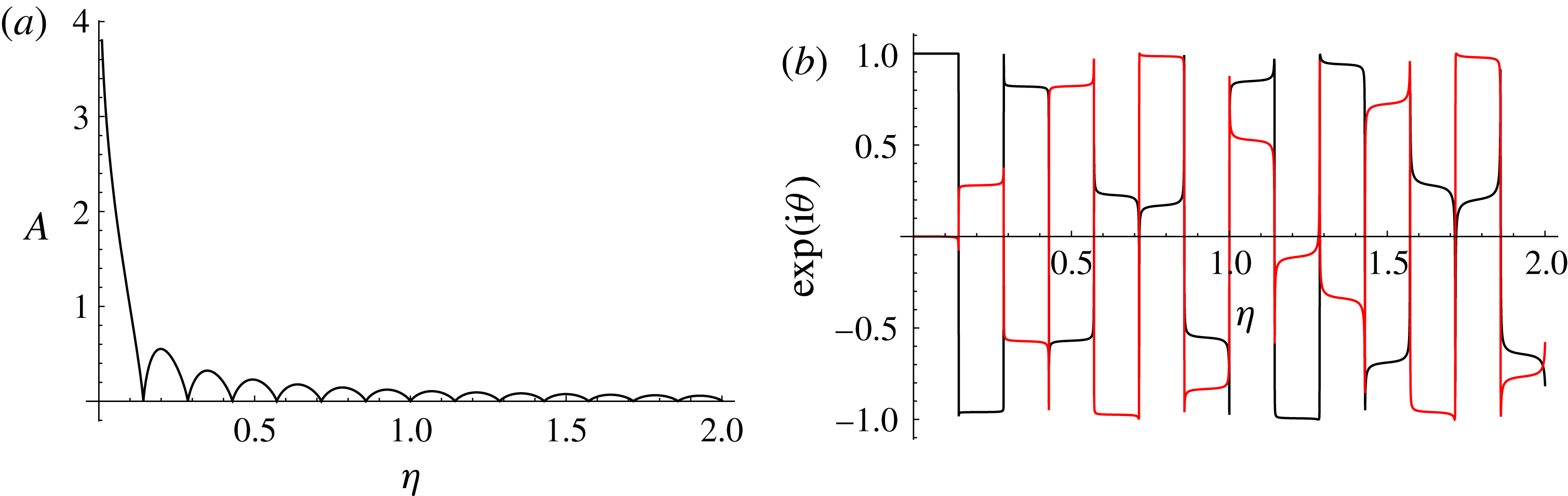
Time evolution of self-similar solutions in intertwining co-rotating vortices, with
 $\unicode[STIX]{x1D713}_{1}(t,s)$
and
 $\unicode[STIX]{x1D713}_{2}(t,s)$
shown in blue and red respectively. Numerical solutions of (3.24) and (3.27), with
 $\unicode[STIX]{x1D708}(t,s)=0$
, are plotted over
 $s\in [0.5,20]$
. In particular, the initial conditions are
 $A(\unicode[STIX]{x1D702}=0.001)=5$
,
 $A^{\prime }(\unicode[STIX]{x1D702}=0.001)=1$
,
 $\unicode[STIX]{x1D703}(\unicode[STIX]{x1D702}=0.001)=0$
and
 $\unicode[STIX]{x1D703}^{\prime }(\unicode[STIX]{x1D702}=0.001)=0$
. The times shown are (a)
 $t=10$
, (b)
 $t=50$
, (c)
 $t=100$
, (d)
 $t=500$
, (e)
 $t=1000$
and (f)
 $t=5000$
.
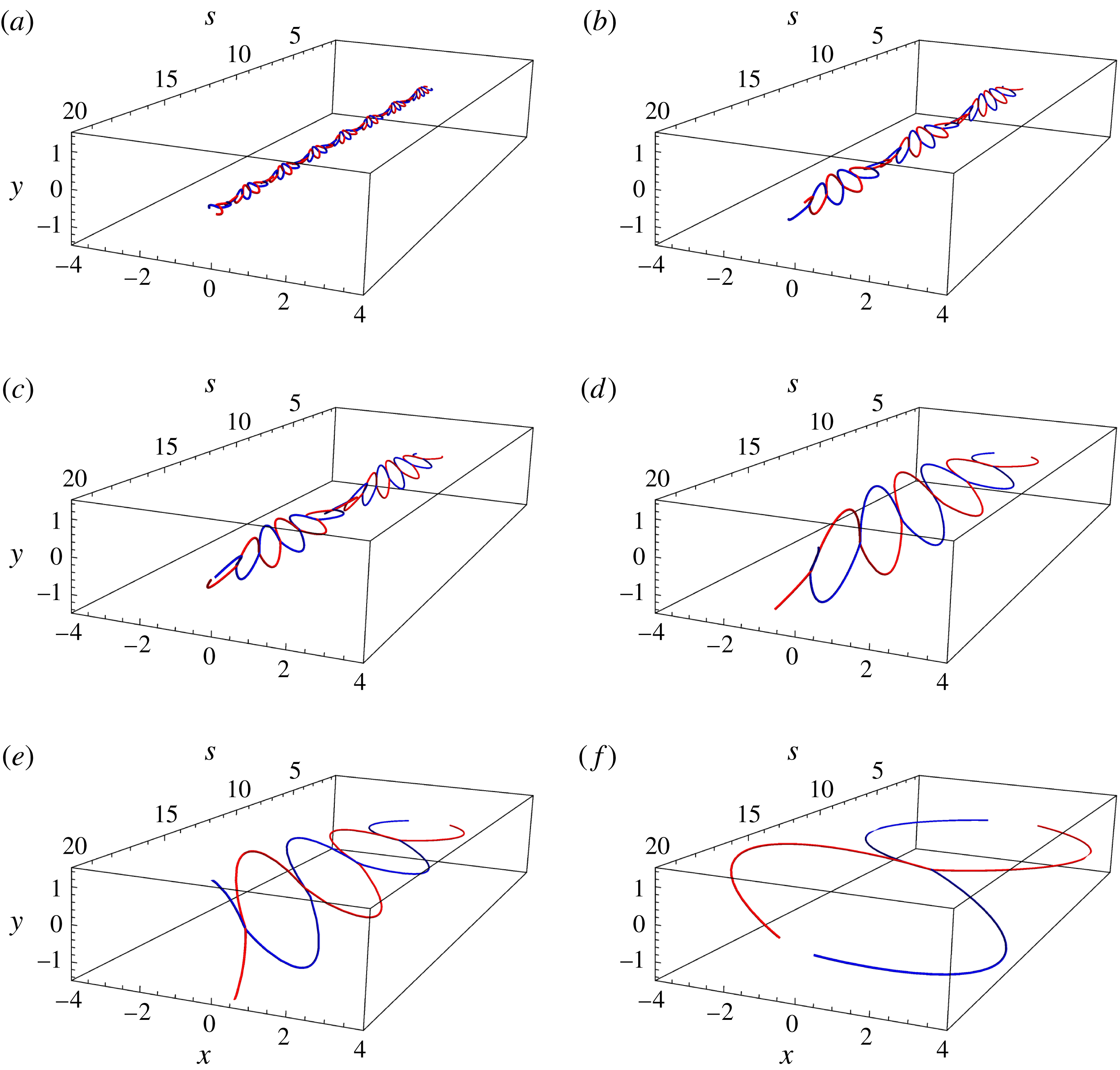
3.2 Counter-rotating vortices
We now study vortex pairs with opposite circulation, so that
 $\unicode[STIX]{x1D6F1}=-1$
. In this case, (3.1) and (3.2) give
 $$\begin{eqnarray}\displaystyle & \displaystyle \text{i}{\displaystyle \frac{\unicode[STIX]{x2202}\unicode[STIX]{x1D708}}{\unicode[STIX]{x2202}t}}-{\displaystyle \frac{\unicode[STIX]{x2202}^{2}\unicode[STIX]{x1D707}}{\unicode[STIX]{x2202}s^{2}}}+{\displaystyle \frac{4\unicode[STIX]{x1D707}}{|\unicode[STIX]{x1D707}|^{2}}}=0, & \displaystyle\end{eqnarray}$$
 $$\begin{eqnarray}\displaystyle & \displaystyle \text{i}{\displaystyle \frac{\unicode[STIX]{x2202}\unicode[STIX]{x1D707}}{\unicode[STIX]{x2202}t}}-{\displaystyle \frac{\unicode[STIX]{x2202}^{2}\unicode[STIX]{x1D708}}{\unicode[STIX]{x2202}s^{2}}}=0. & \displaystyle\end{eqnarray}$$
As in § 2.2, we can rewrite (3.28) and (3.29) as a single partial differential equation for
 $\unicode[STIX]{x1D707}(t,s)$
by supposing the same differentiability constraints on
 $\unicode[STIX]{x1D713}_{1}(t,s)$
and
 $\unicode[STIX]{x1D713}_{2}(t,s)$
,
 $$\begin{eqnarray}{\displaystyle \frac{\unicode[STIX]{x2202}^{2}\unicode[STIX]{x1D707}}{\unicode[STIX]{x2202}t^{2}}}+{\displaystyle \frac{\unicode[STIX]{x2202}^{4}\unicode[STIX]{x1D707}}{\unicode[STIX]{x2202}s^{4}}}-4{\displaystyle \frac{\unicode[STIX]{x2202}^{2}}{\unicode[STIX]{x2202}s^{2}}}\left({\displaystyle \frac{\unicode[STIX]{x1D707}}{|\unicode[STIX]{x1D707}|^{2}}}\right)=0,\end{eqnarray}$$
and subsequently calculate
 $\unicode[STIX]{x1D708}(t,s)$
by solving (3.29).
3.2.1 Plane-wave solutions
We consider solutions to (3.30) of the form given in (3.9). The vortex centre
 $\unicode[STIX]{x1D708}(t,s)$
is not arbitrary in this case, and is explicitly given by solving (3.29),
 $$\begin{eqnarray}\unicode[STIX]{x1D708}(t,s)=-{\displaystyle \frac{\unicode[STIX]{x1D714}}{k^{2}}}A_{0}\text{exp}(\text{i}(ks-\unicode[STIX]{x1D714}t))+c_{1}s+c_{2},\end{eqnarray}$$
for
 $c_{1},c_{2}\in \mathbb{C}$
and where
 $A_{0}$
,
 $k$
and
 $\unicode[STIX]{x1D714}$
have the same meaning as in § 3.1.1. The centre of the pair traces out a helix with the same wavenumber and rotates at the same angular velocity as the separation between the vortex pair, up to an arbitrary orientation determined by
 $c_{1}$
and translation defined by
 $c_{2}$
.
Substitution of (3.9) into (3.30) gives the dispersion relation
 $$\begin{eqnarray}\unicode[STIX]{x1D714}=\pm k\sqrt{k^{2}+{\displaystyle \frac{4}{A_{0}^{2}}}}.\end{eqnarray}$$
The angular velocity is again determined by the wavenumber
 $k$
and the amplitude of vortex separation
 $A_{0}$
. Similarly to § 3.1.1,
 $\unicode[STIX]{x1D714}$
can be positive, negative or zero; however, for all non-zero values, the angular velocity can be either clockwise or anticlockwise rotating, regardless of the parameters imposed on the system. To illustrate, we plot the filament shapes of the vortex pair in figure 17 for
 $A_{0}=1$
with (a,b)
 $k=1$
with
 $\unicode[STIX]{x1D714}=-\sqrt{5}$
, and (c,d)
 $k=1$
with
 $\unicode[STIX]{x1D714}=\sqrt{5}$
. The positive root of (3.32) was taken in both cases.
Time evolution of plane-wave solutions in intertwining counter-rotating vortices, with
 $\unicode[STIX]{x1D713}_{1}(t,s)$
and
 $\unicode[STIX]{x1D713}_{2}(t,s)$
shown in blue and red respectively. In particular, (3.9) and (3.31), with the dispersion relation determined by (3.32), are plotted over
 $s\in [-5,5]$
. The parameters are
 $A_{0}=1$
and (a,b)
 $k=-1$
with
 $\unicode[STIX]{x1D714}=-\sqrt{5}$
and (c,d)
 $k=1$
with
 $\unicode[STIX]{x1D714}=\sqrt{5}$
. The times shown are (a,c)
 $t=0$
and (b,d)
 $t=0.5$
.
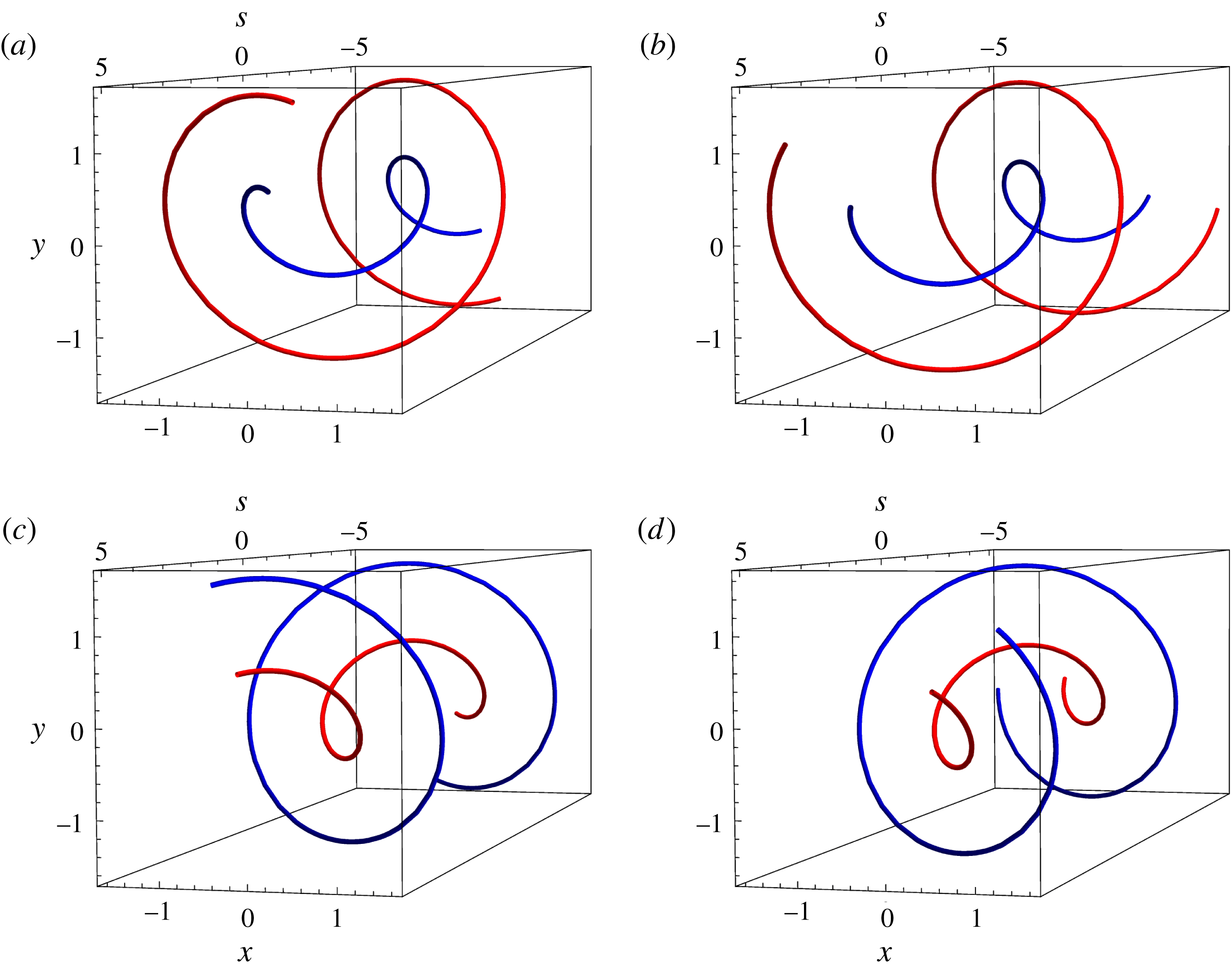
3.2.2 Travelling wave solutions
We transform (3.30) into wave coordinates
 $\unicode[STIX]{x1D709}=s-vt$
and integrate twice with respect to
 $\unicode[STIX]{x1D709}$
to obtain
 $$\begin{eqnarray}{\displaystyle \frac{\text{d}^{2}\unicode[STIX]{x1D707}}{\text{d}\unicode[STIX]{x1D709}^{2}}}+v^{2}\unicode[STIX]{x1D707}-{\displaystyle \frac{4\unicode[STIX]{x1D707}}{|\unicode[STIX]{x1D707}|^{2}}}=\unicode[STIX]{x1D6FF}\end{eqnarray}$$
for
 $\unicode[STIX]{x1D6FF}\in \mathbb{C}$
, which has constraints
 $$\begin{eqnarray}\displaystyle & \displaystyle {\displaystyle \frac{\text{d}^{3}\unicode[STIX]{x1D707}}{\text{d}\unicode[STIX]{x1D709}^{3}}}+v^{2}{\displaystyle \frac{\text{d}\unicode[STIX]{x1D707}}{\text{d}\unicode[STIX]{x1D709}}}-{\displaystyle \frac{\text{d}}{\text{d}\unicode[STIX]{x1D709}}}\left({\displaystyle \frac{4\unicode[STIX]{x1D707}}{|\unicode[STIX]{x1D707}|^{2}}}\right)=0, & \displaystyle\end{eqnarray}$$
 $$\begin{eqnarray}\displaystyle & \displaystyle v^{2}\unicode[STIX]{x1D707}-\text{i}v{\displaystyle \frac{\text{d}\unicode[STIX]{x1D708}}{\text{d}\unicode[STIX]{x1D709}}}=\unicode[STIX]{x1D6FF}. & \displaystyle\end{eqnarray}$$
As before, we determine
 $\unicode[STIX]{x1D6FF}$
by imposing conditions on
 $\unicode[STIX]{x1D707}(\unicode[STIX]{x1D709})$
and
 $\unicode[STIX]{x1D708}^{\prime }(\unicode[STIX]{x1D709})$
. However, for the forthcoming analysis, we only consider cases where
 $\unicode[STIX]{x1D6FF}=0$
.
We study solutions to (3.33) of the amplitude–phase ansatz (3.5) and find, upon separating real and imaginary components,
 $$\begin{eqnarray}\displaystyle & \displaystyle {\displaystyle \frac{\text{d}^{2}A}{\text{d}\unicode[STIX]{x1D709}^{2}}}+v^{2}A-A\left({\displaystyle \frac{\text{d}\unicode[STIX]{x1D703}}{\text{d}\unicode[STIX]{x1D709}}}\right)^{2}-{\displaystyle \frac{4}{A}}=0, & \displaystyle\end{eqnarray}$$
 $$\begin{eqnarray}\displaystyle & \displaystyle {\displaystyle \frac{\text{d}}{\text{d}\unicode[STIX]{x1D709}}}\left(A^{2}{\displaystyle \frac{\text{d}\unicode[STIX]{x1D703}}{\text{d}\unicode[STIX]{x1D709}}}\right)=0. & \displaystyle\end{eqnarray}$$
Solutions to these equations naturally generalise the plane-wave helix solutions of the previous subsection, as those solutions correspond to constant
 $A$
.
We note that (3.36) and (3.37) have an exact solution given by (3.13) with a potential function given by
 $$\begin{eqnarray}V(A)={\displaystyle \frac{v^{2}A^{2}}{2}}-4\ln (A)+{\displaystyle \frac{\unicode[STIX]{x1D6FE}^{2}}{2A^{2}}},\end{eqnarray}$$
where
 $\unicode[STIX]{x1D6FE}\in \mathbb{R}$
is an integration constant that has the same physical meaning as in § 3.1.2, measuring the coupling between the vortex pair separation and its change in orientation.
We note some important differences compared with the co-rotating case. First, if
 $\unicode[STIX]{x1D6FE}=0$
, then the orientation of the counter-rotating pair does not change and the oscillation remains completely planar for all time. For example, vortices that only vibrate in the
 $x$
-axis will do so for all time. Furthermore, the pair no longer collapses as
 $t\rightarrow \infty$
, according to (3.38), as the lower bound of the potential is determined by
 $-4\text{ln}(A)$
in (3.38). For any value of
 $v$
or
 $\unicode[STIX]{x1D6FE}$
, the counter-rotating vortices will not meet; however, if the velocity of the travelling wave solution
 $v=0$
, the pair will repel as
 $A\rightarrow \infty$
for
 $\unicode[STIX]{x1D709}\rightarrow \pm \infty$
. If
 $v\neq 0$
, then periodic solutions in
 $A$
are guaranteed for all values of
 $\unicode[STIX]{x1D6FE}$
. This aspect leads to the counter-rotating vortices having a different asymptotic structure that no longer depends on
 $\unicode[STIX]{x1D6FE}$
, unlike what was previously seen for the co-rotating vortices (see § B.3 for further details).
We illustrate the potential (3.38) and numerically solve (3.36) and (3.37) for
 $A(\unicode[STIX]{x1D709})$
and
 $\unicode[STIX]{x1D703}(\unicode[STIX]{x1D709})$
with the conditions
 $A(\unicode[STIX]{x1D709}=0)=2$
,
 $A^{\prime }(\unicode[STIX]{x1D709}=0)=0$
and
 $\unicode[STIX]{x1D703}(\unicode[STIX]{x1D709}=0)=0$
, for parameters
 $v=2$
and
 $\unicode[STIX]{x1D6FE}=1$
(shown in figures 18
a, 18
b and 18
c respectively). In this case, the trajectories of
 $A$
are restricted such that they always remain within the range
 $A\in [0.494376,2]$
for all
 $t$
and
 $s$
, with period given by
 $T\approx 1.925$
. We note that both figures 18(b) and 18(c) show that the separation of the vortex pair is periodic, which, by (3.35), suggests that the position of the pair centre will periodically oscillate too.
We numerically solve (3.35) to obtain
 $\unicode[STIX]{x1D708}(\unicode[STIX]{x1D709})$
, imposing the condition
 $\unicode[STIX]{x1D708}(\unicode[STIX]{x1D709}=0)=0$
, and plot the associated filament shapes at times
 $t=\{1,1.5,2,2.5\}$
to obtain figures 19(a)–19(d) respectively. Furthermore, we show the shape the vortex pair traces on the
 $x$
–
 $y$
plane, for
 $s=0$
during the time
 $t\in [0,25]$
, in figure 20. We observe that
 $\unicode[STIX]{x1D713}_{2}(t,s)$
oscillates in a trefoil knot-like shape while
 $\unicode[STIX]{x1D713}_{1}(t,s)$
traces out a helical shape that is deformed such that its curvature minima coincide with the maximal tips of the trefoil shape, a result that arises due to the coupling of
 $\unicode[STIX]{x1D707}(t,s)$
and
 $\unicode[STIX]{x1D708}(t,s)$
, which causes the centre of the vortex pair to form the periodically deformed helical shape for all time and filament arclength.
(a) Potential of the separation equation as defined in (3.38), and numerical solutions of (b)
 $A(\unicode[STIX]{x1D709})$
and (c) the real and imaginary parts of the complex exponential
 $\text{exp}(\text{i}\unicode[STIX]{x1D703}(\unicode[STIX]{x1D709}))$
(shown in black and red respectively) obtained by solving (3.37) and (3.36) for
 $v=2$
,
 $\unicode[STIX]{x1D6FE}=1$
and
 $\unicode[STIX]{x1D6FF}=0$
with initial conditions
 $A(\unicode[STIX]{x1D709}=0)=2$
,
 $A^{\prime }(\unicode[STIX]{x1D709}=0)=0$
and
 $\unicode[STIX]{x1D703}(\unicode[STIX]{x1D709}=0)=0$
. The trajectories of
 $A$
are restricted in the potential well such that they never exceed the potential
 $2v^{2}/8-4\ln (2)+\unicode[STIX]{x1D6FE}^{2}/8$
, shown by the dashed line, and oscillate with period
 $T\approx 1.925$
according to (3.13).
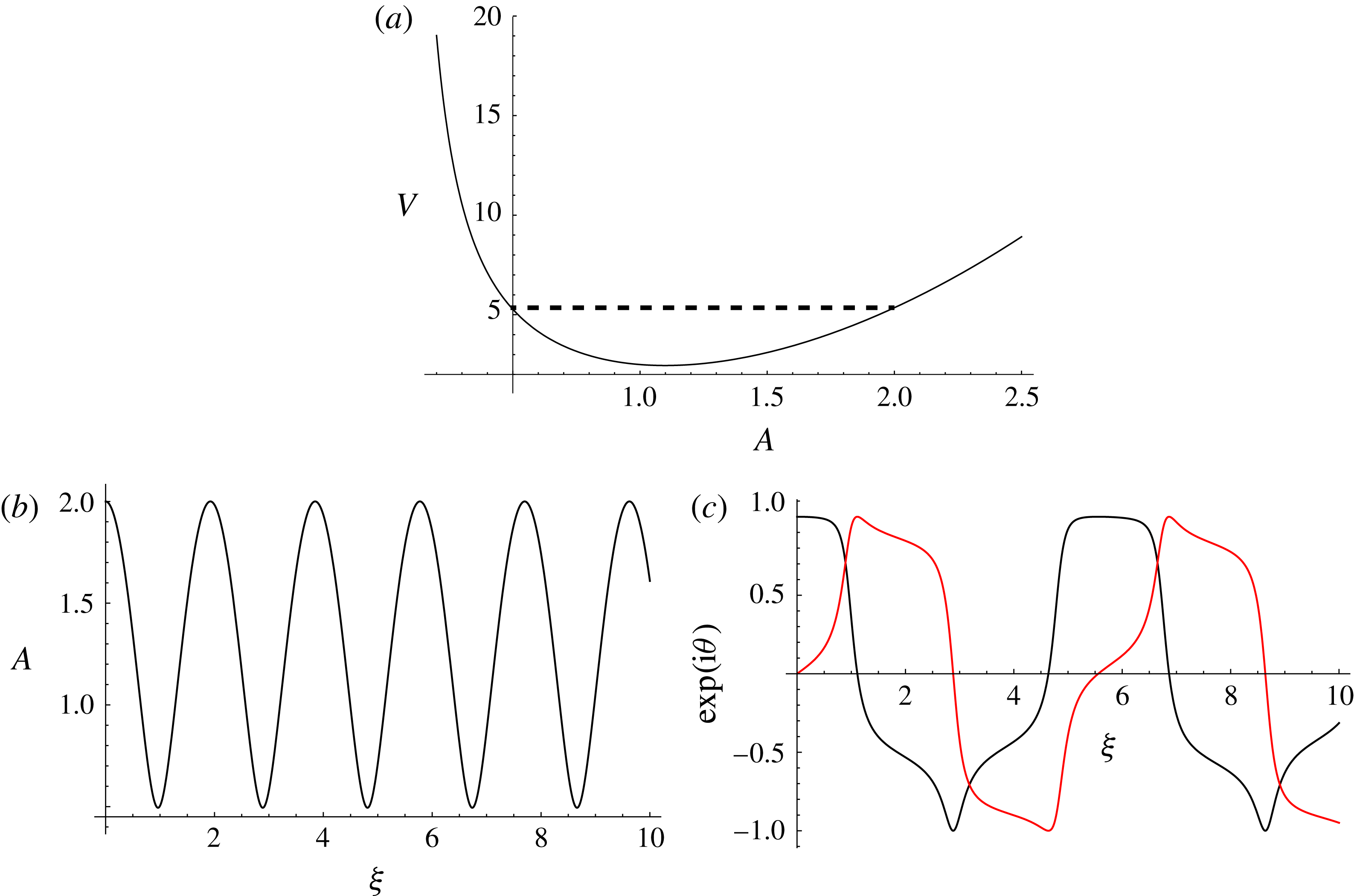
Time evolution of travelling wave solutions in intertwining counter-rotating vortices, with
 $\unicode[STIX]{x1D713}_{1}(t,s)$
and
 $\unicode[STIX]{x1D713}_{2}(t,s)$
shown in blue and red respectively. Numerical solutions of (3.35), (3.37) and (3.36) are plotted over
 $s\in [0,10]$
. In particular, the initial conditions are
 $A(\unicode[STIX]{x1D709}=0)=2$
,
 $A^{\prime }(\unicode[STIX]{x1D709}=0)=0$
,
 $\unicode[STIX]{x1D703}(\unicode[STIX]{x1D709}=0)=0$
and
 $\unicode[STIX]{x1D708}(\unicode[STIX]{x1D709}=0)=0$
with parameters
 $v=2$
,
 $\unicode[STIX]{x1D6FE}=1$
and
 $\unicode[STIX]{x1D6FF}=0$
. The times shown are (a)
 $t=0$
, (b)
 $t=2$
, (c)
 $t=4$
and (d)
 $t=8$
.
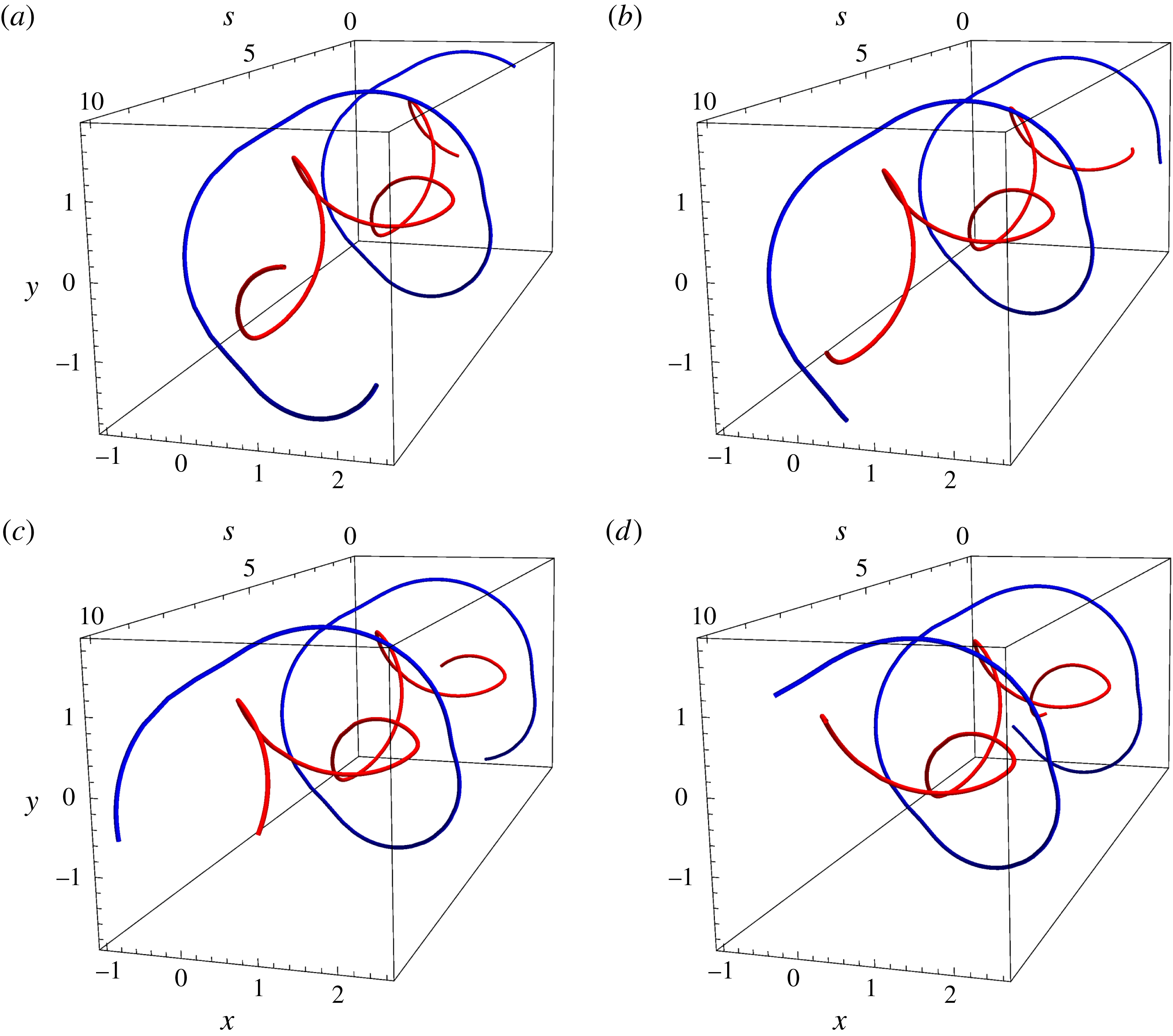
The shape that the filament pair in figure 19 traces out in the
 $x$
–
 $y$
plane during the time
 $t\in [0,25]$
at
 $s=0$
, with
 $\unicode[STIX]{x1D713}_{1}(t,s)$
and
 $\unicode[STIX]{x1D713}_{2}(t,s)$
corresponding to black and red lines respectively.
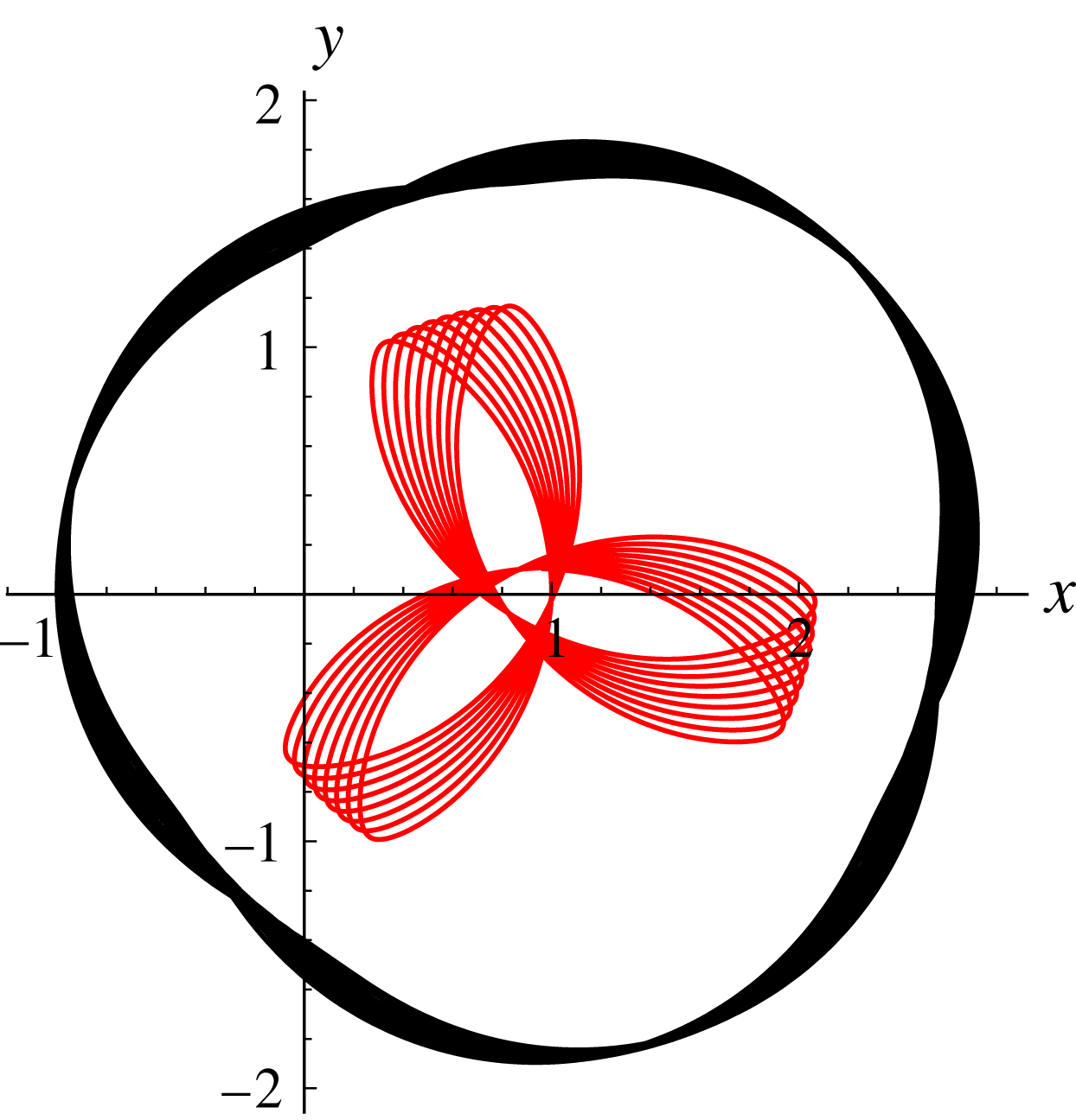
3.2.3 Purely rotating-wave solutions
We study solutions of the rotating-wave ansatz of (3.5), (3.17) and (3.18) and apply it to (3.30) to obtain
 $$\begin{eqnarray}{\displaystyle \frac{\text{d}^{4}A}{\text{d}s^{4}}}-\unicode[STIX]{x1D714}^{2}A-{\displaystyle \frac{\text{d}^{2}}{\text{d}s^{2}}}\left({\displaystyle \frac{4}{A}}\right)=0,\end{eqnarray}$$
where the general solution to
 $\unicode[STIX]{x1D708}(t,s)$
is given by a combination (3.28) and (3.29) as
 $$\begin{eqnarray}\unicode[STIX]{x1D708}(t,s)={\displaystyle \frac{1}{\unicode[STIX]{x1D714}}}\left({\displaystyle \frac{\text{d}^{2}A}{\text{d}s^{2}}}-{\displaystyle \frac{4}{A}}\right)\text{exp}(-\text{i}\unicode[STIX]{x1D714}t)+c_{1}s+c_{2},\end{eqnarray}$$
for
 $c_{1},c_{2}\in \mathbb{C}$
. Again, the solutions we obtain will correspond to planar vortex filaments that maintain their spatial form as the only motion is purely rotational.
We observe that, with the characteristic coupling between the deviations and the centre of the counter-rotating vortices, the pair not only rotate around each other, but also around a centre point in the fluid, determined by the conditions on
 $\unicode[STIX]{x1D708}(t,s)$
.
We numerically solve (3.39) and (3.40) with boundary conditions given by
 $A(s=0)=2$
,
 $A(s=10)=2$
,
 $A^{\prime }(s=0)=0$
,
 $A^{\prime }(s=10)=0$
and
 $\unicode[STIX]{x1D708}(t,0)=\unicode[STIX]{x2202}\unicode[STIX]{x1D708}(t,0)/\unicode[STIX]{x2202}s=0$
, with
 $\unicode[STIX]{x1D714}=0.5$
and
 $c_{1}=c_{2}=0$
. We plot
 $\unicode[STIX]{x1D707}(t,s)$
and
 $\unicode[STIX]{x1D708}(t,s)$
at
 $t=0$
in figure 21(a,b), and the corresponding filament shapes over
 $s\in [0,10]$
at times
 $t=\{2.5,7.5\}$
in figure 21(c,d). We observe that, for the boundary conditions chosen, the separation of the vortex pair is oscillatory along the arclength (figure 21
a), a solution not possible for the co-rotating case seen in § 3.1.3. By (3.40),
 $\unicode[STIX]{x1D708}(t,s)$
is also bounded and non-zero (figure 21
b). The filament shapes are therefore asymmetrical when compared with the symmetrical co-rotating vortices (figure 21), a direct result of the coupling of
 $\unicode[STIX]{x1D707}(t,s)$
and
 $\unicode[STIX]{x1D708}(t,s)$
in counter-rotating vortices.
Numerical solutions of (3.39) and (3.40) at
 $t=0$
(shown in (a,b)) for the conditions
 $A(s=0)=2$
,
 $A(s=10)=2$
,
 $A^{\prime }(s=0)=0$
,
 $A^{\prime }(s=10)=0$
and
 $\unicode[STIX]{x1D708}(t,0)=\unicode[STIX]{x2202}\unicode[STIX]{x1D708}(t,0)/\unicode[STIX]{x2202}s=0$
, with
 $\unicode[STIX]{x1D714}=0.5$
and
 $c_{1}=c_{2}=0$
. The corresponding filament shapes of
 $\unicode[STIX]{x1D713}_{1}(t,s)$
(shown in blue) and
 $\unicode[STIX]{x1D713}_{2}(t,s)$
(shown in red) are plotted over
 $s\in [0,10]$
for times (c)
 $t=2.5$
and (d)
 $t=7.5$
. The solutions clearly take on a planar filament structure.
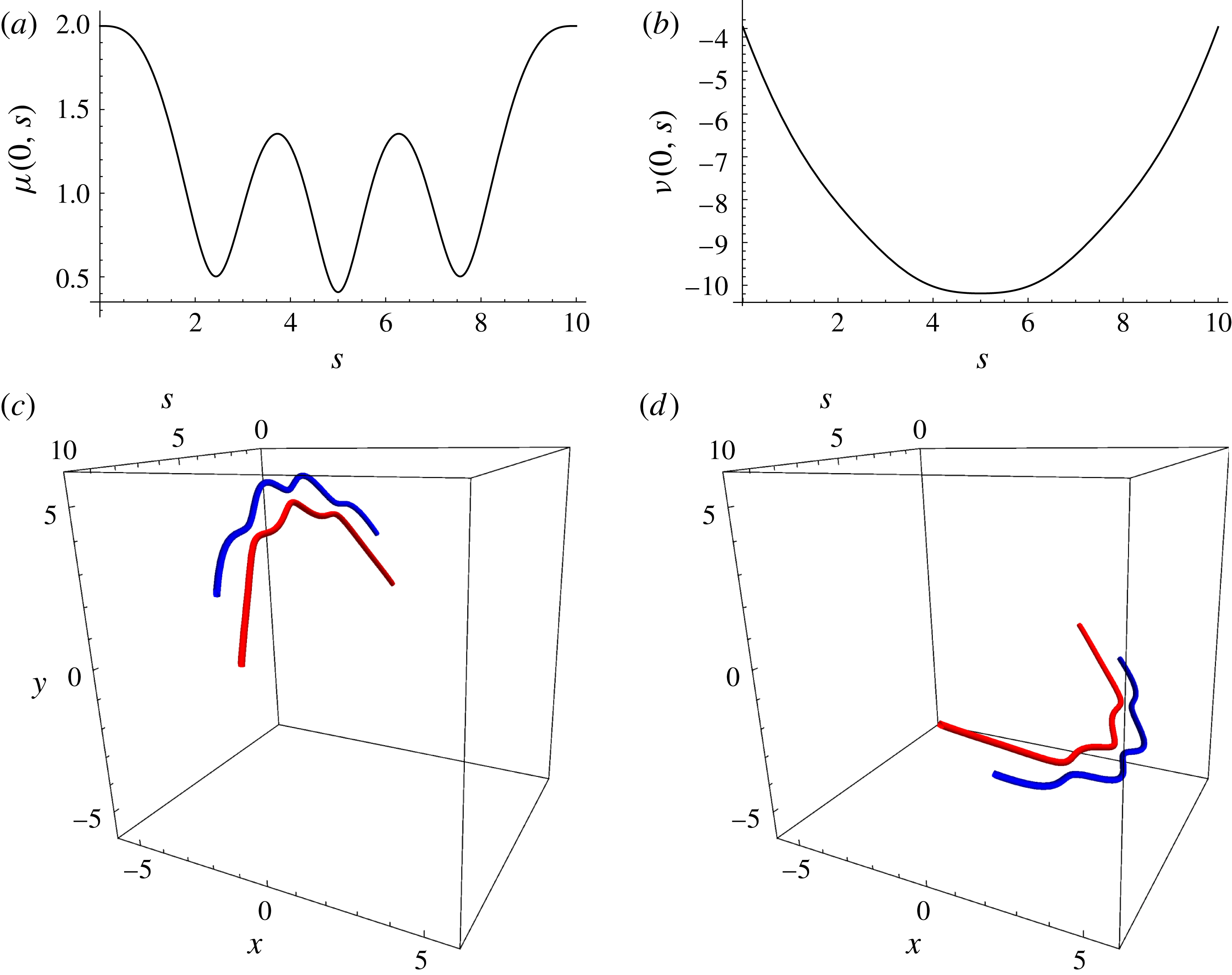
3.2.4 Self-similar solutions
We transform (3.28) and (3.29) into the variables
 $\unicode[STIX]{x1D707}(t,s)=s\unicode[STIX]{x1D712}(\unicode[STIX]{x1D702})$
and
 $\unicode[STIX]{x1D708}(t,s)=s\unicode[STIX]{x1D70C}(\unicode[STIX]{x1D702})$
, for
 $\unicode[STIX]{x1D702}=s/\sqrt{t}$
, to find
 $$\begin{eqnarray}\displaystyle & \displaystyle -{\displaystyle \frac{\text{i}\unicode[STIX]{x1D702}^{3}}{2}}{\displaystyle \frac{\text{d}\unicode[STIX]{x1D70C}}{\text{d}\unicode[STIX]{x1D702}}}-\unicode[STIX]{x1D702}^{2}{\displaystyle \frac{\text{d}^{2}\unicode[STIX]{x1D712}}{\text{d}\unicode[STIX]{x1D702}^{2}}}-2\unicode[STIX]{x1D702}{\displaystyle \frac{\text{d}\unicode[STIX]{x1D712}}{\text{d}\unicode[STIX]{x1D702}}}+{\displaystyle \frac{4\unicode[STIX]{x1D712}}{|\unicode[STIX]{x1D712}|^{2}}}=0, & \displaystyle\end{eqnarray}$$
 $$\begin{eqnarray}\displaystyle & \displaystyle -{\displaystyle \frac{\text{i}\unicode[STIX]{x1D702}^{3}}{2}}{\displaystyle \frac{\text{d}\unicode[STIX]{x1D712}}{\text{d}\unicode[STIX]{x1D702}}}-{\displaystyle \frac{\text{d}}{\text{d}\unicode[STIX]{x1D702}}}\left(\unicode[STIX]{x1D702}^{2}{\displaystyle \frac{\text{d}\unicode[STIX]{x1D70C}}{\text{d}\unicode[STIX]{x1D702}}}\right)=0, & \displaystyle\end{eqnarray}$$
and a single equation for
 $\unicode[STIX]{x1D712}(\unicode[STIX]{x1D702})$
upon substituting (3.41) into (3.42),
 $$\begin{eqnarray}\unicode[STIX]{x1D702}{\displaystyle \frac{\text{d}^{3}\unicode[STIX]{x1D712}}{\text{d}\unicode[STIX]{x1D702}^{3}}}+3{\displaystyle \frac{\text{d}^{2}\unicode[STIX]{x1D712}}{\text{d}\unicode[STIX]{x1D702}^{2}}}+{\displaystyle \frac{\unicode[STIX]{x1D702}^{3}}{4}}{\displaystyle \frac{\text{d}\unicode[STIX]{x1D712}}{\text{d}\unicode[STIX]{x1D702}}}-{\displaystyle \frac{4}{\unicode[STIX]{x1D702}}}{\displaystyle \frac{\text{d}}{\text{d}\unicode[STIX]{x1D702}}}\left({\displaystyle \frac{\unicode[STIX]{x1D712}}{|\unicode[STIX]{x1D712}|^{2}}}\right)+{\displaystyle \frac{4}{\unicode[STIX]{x1D702}^{2}}}\left({\displaystyle \frac{\unicode[STIX]{x1D712}}{|\unicode[STIX]{x1D712}|^{2}}}\right)=0,\end{eqnarray}$$
with the additional initial condition
 $\unicode[STIX]{x1D712}^{\prime \prime }(\unicode[STIX]{x1D702})$
obtained from (3.41) using conditions on
 $\unicode[STIX]{x1D712}(\unicode[STIX]{x1D702})$
,
 $\unicode[STIX]{x1D712}^{\prime }(\unicode[STIX]{x1D702})$
and
 $\unicode[STIX]{x1D70C}^{\prime }(\unicode[STIX]{x1D702})$
.
We study solutions to
 $\unicode[STIX]{x1D712}(\unicode[STIX]{x1D702})$
of the amplitude–phase ansatz in (3.23) and find, upon substitution into (3.43) and separating real and imaginary parts,
 $$\begin{eqnarray}\displaystyle & & \displaystyle \unicode[STIX]{x1D702}{\displaystyle \frac{\text{d}^{3}A}{\text{d}\unicode[STIX]{x1D702}^{3}}}-3\unicode[STIX]{x1D702}A{\displaystyle \frac{\text{d}\unicode[STIX]{x1D703}}{\text{d}\unicode[STIX]{x1D702}}}{\displaystyle \frac{\text{d}^{2}\unicode[STIX]{x1D703}}{\text{d}\unicode[STIX]{x1D702}^{2}}}-3\unicode[STIX]{x1D702}{\displaystyle \frac{\text{d}A}{\text{d}\unicode[STIX]{x1D702}}}\left({\displaystyle \frac{\text{d}\unicode[STIX]{x1D703}}{\text{d}\unicode[STIX]{x1D702}}}\right)^{2}+3{\displaystyle \frac{\text{d}^{2}A}{\text{d}\unicode[STIX]{x1D702}^{2}}}-3A\left({\displaystyle \frac{\text{d}\unicode[STIX]{x1D703}}{\text{d}\unicode[STIX]{x1D702}}}\right)^{2}\nonumber\\ \displaystyle & & \displaystyle \qquad +\,{\displaystyle \frac{\unicode[STIX]{x1D702}^{3}}{4}}{\displaystyle \frac{\text{d}A}{\text{d}\unicode[STIX]{x1D702}}}+{\displaystyle \frac{4}{\unicode[STIX]{x1D702}A^{2}}}{\displaystyle \frac{\text{d}A}{\text{d}\unicode[STIX]{x1D702}}}+{\displaystyle \frac{4}{\unicode[STIX]{x1D702}^{2}A}}=0,\end{eqnarray}$$
 $$\begin{eqnarray}\displaystyle & & \displaystyle \unicode[STIX]{x1D702}A{\displaystyle \frac{\text{d}^{3}\unicode[STIX]{x1D703}}{\text{d}\unicode[STIX]{x1D702}^{3}}}+3\unicode[STIX]{x1D702}{\displaystyle \frac{\text{d}A}{\text{d}\unicode[STIX]{x1D702}}}{\displaystyle \frac{\text{d}^{2}\unicode[STIX]{x1D703}}{\text{d}\unicode[STIX]{x1D702}^{2}}}+3\unicode[STIX]{x1D702}{\displaystyle \frac{\text{d}\unicode[STIX]{x1D703}}{\text{d}\unicode[STIX]{x1D702}}}{\displaystyle \frac{\text{d}^{2}A}{\text{d}\unicode[STIX]{x1D702}^{2}}}-\unicode[STIX]{x1D702}A\left({\displaystyle \frac{\text{d}\unicode[STIX]{x1D703}}{\text{d}\unicode[STIX]{x1D702}}}\right)^{3}+6{\displaystyle \frac{\text{d}A}{\text{d}\unicode[STIX]{x1D702}}}{\displaystyle \frac{\text{d}\unicode[STIX]{x1D703}}{\text{d}\unicode[STIX]{x1D702}}}\nonumber\\ \displaystyle & & \displaystyle \qquad +\,3A{\displaystyle \frac{\text{d}^{2}\unicode[STIX]{x1D703}}{\text{d}\unicode[STIX]{x1D702}^{2}}}+{\displaystyle \frac{\unicode[STIX]{x1D702}^{3}A}{4}}{\displaystyle \frac{\text{d}\unicode[STIX]{x1D703}}{\text{d}\unicode[STIX]{x1D702}}}-{\displaystyle \frac{4\unicode[STIX]{x1D702}}{A}}{\displaystyle \frac{\text{d}\unicode[STIX]{x1D703}}{\text{d}\unicode[STIX]{x1D702}}}=0.\end{eqnarray}$$
To obtain physical intuition into the types of solutions predicted by (3.43), we numerically solve (3.44) and (3.45) with the conditions
 $A(\unicode[STIX]{x1D702}=3)=1$
,
 $A^{\prime }(\unicode[STIX]{x1D702}=3)=0$
,
 $A^{\prime \prime }(\unicode[STIX]{x1D702}=3)=0$
,
 $\unicode[STIX]{x1D703}(\unicode[STIX]{x1D702}=3)=0$
,
 $\unicode[STIX]{x1D703}^{\prime }(\unicode[STIX]{x1D702}=3)=1$
and
 $\unicode[STIX]{x1D703}^{\prime \prime }(\unicode[STIX]{x1D702}=1)=-5$
, and plot the real and imaginary parts of
 $\unicode[STIX]{x1D712}(\unicode[STIX]{x1D702})$
and
 $\unicode[STIX]{x1D70C}(\unicode[STIX]{x1D702})$
, using the condition
 $\unicode[STIX]{x1D70C}(\unicode[STIX]{x1D702}=3)=0$
, in figures 22(a), 22(b) and 22(c), 22(d) respectively. Furthermore, we illustrate the corresponding filament shapes over the arclength
 $s\in [5,15]$
at times
 $t=\{0.1,1,2,2.5\}$
in figure 23. We observe some parallels to self-similar solutions in other vortex configurations (i.e. § 2.1.2, 2.2.2, and 3.1.4), namely the progression of the vortex pair shape from a straight filament in some orientation to oscillatory solutions with increasing amplitude and wavelength as
 $t\rightarrow \infty$
. However, in contrast to the self-similar solutions in § 3.1.4, the vortices are never in very close proximity, so that the orientation of the pair does not rapidly change according to the dependence of
 $1/A$
in (3.45). The vortex pair remains separated due to the constant offset in
 $\unicode[STIX]{x1D70C}(\unicode[STIX]{x1D702})$
in figure 22(c,d), but as
 $t\rightarrow \infty$
, the centre of the vortex pair moves such that the filaments begin to intertwine and rotate around each other (figure 23
d).
Real and imaginary components of
 $\unicode[STIX]{x1D712}(\unicode[STIX]{x1D702})$
and
 $\unicode[STIX]{x1D70C}(\unicode[STIX]{x1D702})$
calculated by the numerical solution of (3.44), (3.45) and (3.42). The initial conditions are
 $A(\unicode[STIX]{x1D702}=3)=1$
,
 $A^{\prime }(\unicode[STIX]{x1D702}=3)=0$
,
 $A^{\prime \prime }(\unicode[STIX]{x1D702}=3)=0$
,
 $\unicode[STIX]{x1D703}(\unicode[STIX]{x1D702}=3)=0$
,
 $\unicode[STIX]{x1D703}^{\prime }(\unicode[STIX]{x1D702}=3)=1$
,
 $\unicode[STIX]{x1D703}^{\prime \prime }(\unicode[STIX]{x1D702}=3)=-5$
and
 $\unicode[STIX]{x1D70C}(\unicode[STIX]{x1D702}=3)=0$
.
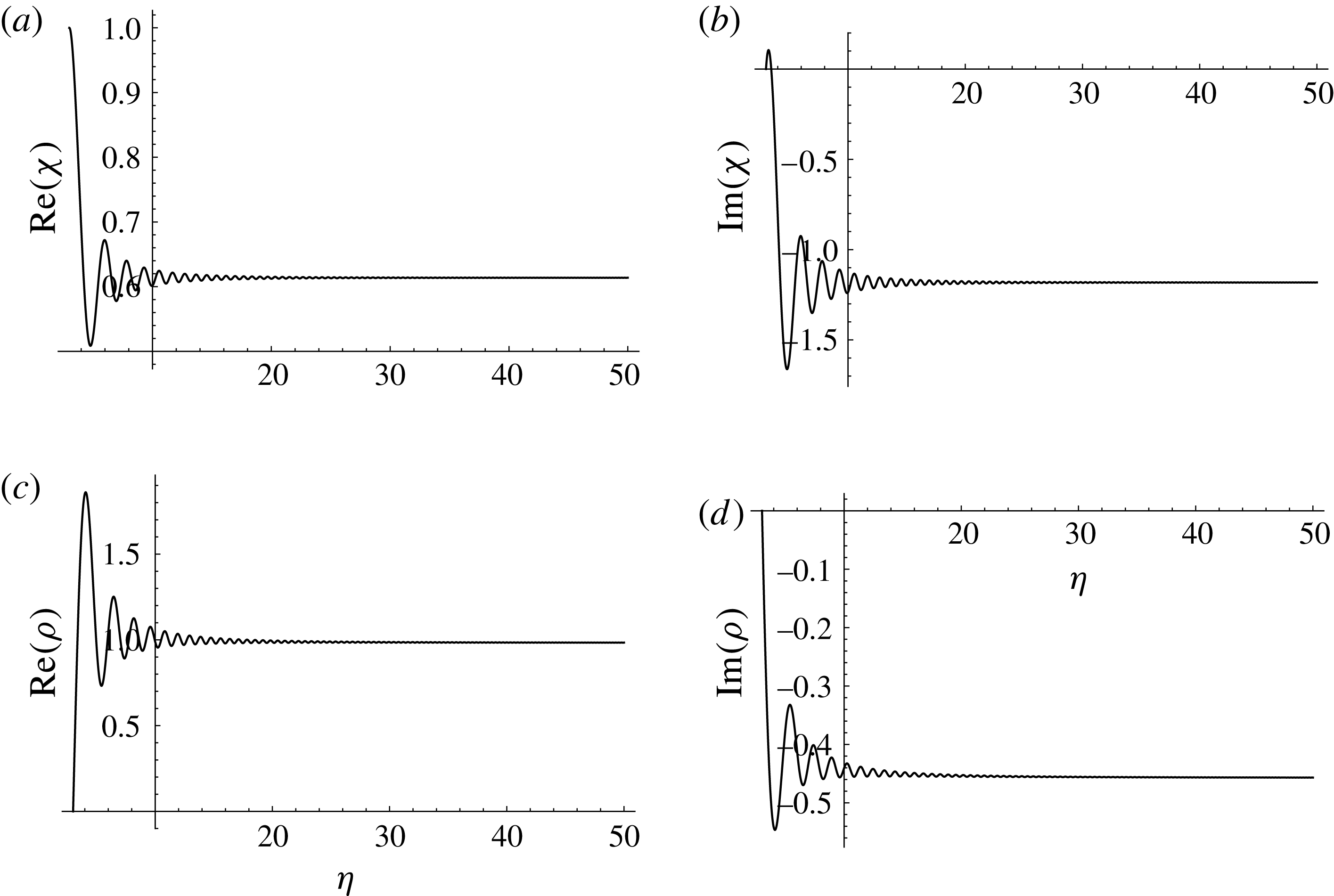
Time evolution of self-similar solutions in intertwining counter-rotating vortices, with
 $\unicode[STIX]{x1D713}_{1}(t,s)$
and
 $\unicode[STIX]{x1D713}_{2}(t,s)$
shown in blue and red respectively. Numerical solutions of (3.44), (3.45) and (3.42) are plotted over
 $s\in [5,15]$
with the initial conditions
 $A(\unicode[STIX]{x1D702}=3)=1$
,
 $A^{\prime }(\unicode[STIX]{x1D702}=3)=0$
,
 $A^{\prime \prime }(\unicode[STIX]{x1D702}=3)=0$
,
 $\unicode[STIX]{x1D703}(\unicode[STIX]{x1D702}=3)=0$
,
 $\unicode[STIX]{x1D703}^{\prime }(\unicode[STIX]{x1D702}=3)=1$
,
 $\unicode[STIX]{x1D703}^{\prime \prime }(\unicode[STIX]{x1D702}=3)=-5$
and
 $\unicode[STIX]{x1D70C}(\unicode[STIX]{x1D702}=3)=0$
. The times shown are (a)
 $t=0.1$
, (b)
 $t=1$
, (c)
 $t=2$
and (d)
 $t=2.5$
.
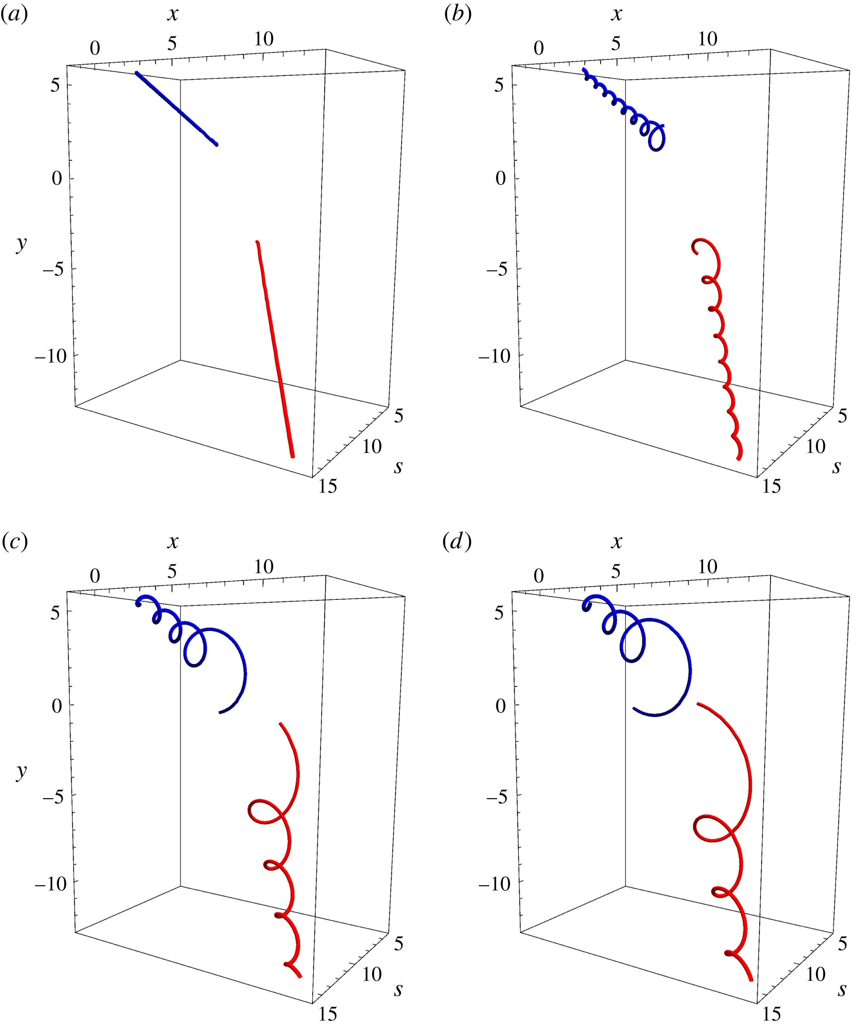
4 Co-rotating vortex hierarchy
We generalise the intertwining vortex coordinates introduced in § 3 to study
 $N$
co-rotating vortices around a central filament, all of which have the same size
 $\unicode[STIX]{x1D6FC}$
and circulation
 $\unicode[STIX]{x1D6E4}$
. We denote the central filament by
 $\unicode[STIX]{x1D713}_{0}(t,s)\in \mathbb{C}$
and the satellite vortices that revolve around this central filament by
 $\unicode[STIX]{x1D713}_{n}(t,s)\in \mathbb{C}$
for
 $n\in \{1,\ldots ,N\}$
. We transform
 $\unicode[STIX]{x1D713}_{0}(t,s)$
and
 $\unicode[STIX]{x1D713}_{n}(t,s)$
into coordinates describing the centre of the vortex hierarchy and the deviations from this centre by defining new variables
 $\unicode[STIX]{x1D708}(t,s)$
and
 $\unicode[STIX]{x1D707}_{n}(t,s)$
, which satisfy
 $$\begin{eqnarray}\displaystyle & \displaystyle \unicode[STIX]{x1D708}=\mathop{\sum }_{j=0}^{N}\unicode[STIX]{x1D713}_{j}, & \displaystyle\end{eqnarray}$$
 $$\begin{eqnarray}\displaystyle & \displaystyle \unicode[STIX]{x1D707}_{n}=\unicode[STIX]{x1D713}_{0}-\unicode[STIX]{x1D713}_{n}, & \displaystyle\end{eqnarray}$$
so that:
 $$\begin{eqnarray}\displaystyle & \displaystyle \unicode[STIX]{x1D713}_{0}={\displaystyle \frac{1}{N+1}}\left(\unicode[STIX]{x1D708}+\mathop{\sum }_{j=1}^{N}\unicode[STIX]{x1D707}_{j}\right), & \displaystyle\end{eqnarray}$$
 $$\begin{eqnarray}\displaystyle & \displaystyle \unicode[STIX]{x1D713}_{n}={\displaystyle \frac{1}{N+1}}\left(\unicode[STIX]{x1D708}-N\unicode[STIX]{x1D707}_{n}+\mathop{\sum }_{j=1}^{N}\unicode[STIX]{x1D707}_{j}\right). & \displaystyle\end{eqnarray}$$
Using (4.3) and (4.4), we obtain the following system of
 $N+1$
equations from (1.1):
 $$\begin{eqnarray}\displaystyle & \displaystyle \text{i}{\displaystyle \frac{\unicode[STIX]{x2202}\unicode[STIX]{x1D708}}{\unicode[STIX]{x2202}\unicode[STIX]{x1D70F}}}+\unicode[STIX]{x1D6FC}\unicode[STIX]{x1D6E4}{\displaystyle \frac{\unicode[STIX]{x2202}^{2}\unicode[STIX]{x1D708}}{\unicode[STIX]{x2202}S^{2}}}=0, & \displaystyle\end{eqnarray}$$
 $$\begin{eqnarray}\displaystyle & \displaystyle \text{i}{\displaystyle \frac{\unicode[STIX]{x2202}\unicode[STIX]{x1D707}_{n}}{\unicode[STIX]{x2202}t}}+\unicode[STIX]{x1D6FC}\unicode[STIX]{x1D6E4}{\displaystyle \frac{\unicode[STIX]{x2202}^{2}\unicode[STIX]{x1D707}_{n}}{\unicode[STIX]{x2202}s^{2}}}+{\displaystyle \frac{4\unicode[STIX]{x1D6E4}\unicode[STIX]{x1D707}_{n}}{|\unicode[STIX]{x1D707}_{n}|^{2}}}+2\unicode[STIX]{x1D6E4}\mathop{\sum }_{j\neq n}\left[{\displaystyle \frac{\unicode[STIX]{x1D707}_{j}}{|\unicode[STIX]{x1D707}_{j}|^{2}}}+{\displaystyle \frac{\unicode[STIX]{x1D707}_{n}-\unicode[STIX]{x1D707}_{j}}{|\unicode[STIX]{x1D707}_{n}-\unicode[STIX]{x1D707}_{j}|^{2}}}\right]=0. & \displaystyle\end{eqnarray}$$
The third term in (4.6) describes the effect of interactions between the satellite vortex
 $\unicode[STIX]{x1D713}_{n}(t,s)$
and the central filament
 $\unicode[STIX]{x1D713}_{0}(t,s)$
. However, there are additional vortex interactions that play a role in the shaping of an individual filament, namely those occurring between the central filament and the other satellites (i.e. fourth term) as well as the interactions between the satellite vortices themselves (i.e. fifth term).
4.1 Plane-wave solutions
To determine the role of these other interactions, we consider plane-wave solutions to (4.6) of the form
 $$\begin{eqnarray}\unicode[STIX]{x1D707}_{n}=B_{n}\text{exp}(\text{i}(k_{n}s-\unicode[STIX]{x1D714}_{n}t+\unicode[STIX]{x1D703}_{n})),\end{eqnarray}$$
where
 $B_{n}$
is the amplitude of the separation between the central and satellite filaments,
 $k_{n}$
is the wavenumber of oscillation,
 $\unicode[STIX]{x1D714}_{n}$
is its angular velocity and
 $\unicode[STIX]{x1D703}_{n}$
is a constant phase offset specifying the initial angular separation from the positive
 $x$
-axis, all of which are constant and real for
 $n\in \{1,\ldots ,N\}$
.
For the case of
 $B_{n}=B$
,
 $k_{n}=k$
,
 $\unicode[STIX]{x1D714}_{n}=\unicode[STIX]{x1D714}$
, and the vortices being evenly distributed around the centre, we obtain the following dispersion relation (see appendix C):
 $$\begin{eqnarray}\unicode[STIX]{x1D714}=\unicode[STIX]{x1D6FC}\unicode[STIX]{x1D6E4}k^{2}-{\displaystyle \frac{\unicode[STIX]{x1D6E4}}{B^{2}}}(N+1),\end{eqnarray}$$
for
 $N\geqslant 2$
.
Setting
 $\unicode[STIX]{x1D6FC}=\unicode[STIX]{x1D6E4}=1$
, we note that the angular velocity of the vortex configuration depends on the wavenumber
 $k$
, the distance of the satellite vortices from the central filament
 $B$
and the number of satellite vortices
 $N$
. Even though we have not specified the direction in which individual vortices rotate (i.e. we have only set their circulations relative to one another and we have not rescaled time), the vortices can rotate clockwise, anticlockwise or not at all, depending only on the aforementioned parameters. The inclusion of more satellite vortices will lead to the system rotating in a clockwise direction with increasing angular velocity.
It is interesting to note that (4.8) has explicit dependence on the vortex core size, which is absent from the dispersion relations found by Boersma & Wood (Reference Boersma and Wood1999) and Okulov (Reference Okulov2004), who considered infinitesimally thin vortex filaments. However, their solutions would be valid for larger values of the wavenumber
 $k$
.
We determine the effect of perturbations to the plane-wave solutions for the simplest case of
 $N=2$
. In particular, we use the ansatz
 $$\begin{eqnarray}\displaystyle & \displaystyle \unicode[STIX]{x1D707}_{1}(t,s)=B\exp (\text{i}(ks-\unicode[STIX]{x1D714}t))+\unicode[STIX]{x1D716}\unicode[STIX]{x1D706}_{1}(t,s), & \displaystyle\end{eqnarray}$$
 $$\begin{eqnarray}\displaystyle & \displaystyle \unicode[STIX]{x1D707}_{2}(t,s)=B\exp (\text{i}(ks-\unicode[STIX]{x1D714}t+\unicode[STIX]{x03C0}))+\unicode[STIX]{x1D716}\unicode[STIX]{x1D706}_{2}(t,s), & \displaystyle\end{eqnarray}$$
for
 $\unicode[STIX]{x1D706}_{1},\unicode[STIX]{x1D706}_{2}\in \mathbb{C}$
and
 $\unicode[STIX]{x1D716}\ll 1$
.
On substituting (4.9) and (4.10) into (4.6), we find that the
 $O(\unicode[STIX]{x1D716}^{0})$
terms give the dispersion relation (4.8) for
 $N=2$
, while to
 $O(\unicode[STIX]{x1D716}^{1})$
,
 $$\begin{eqnarray}\displaystyle & \displaystyle \text{i}{\displaystyle \frac{\unicode[STIX]{x2202}\unicode[STIX]{x1D706}_{1}}{\unicode[STIX]{x2202}t}}+\unicode[STIX]{x1D6FC}\unicode[STIX]{x1D6E4}{\displaystyle \frac{\unicode[STIX]{x2202}^{2}\unicode[STIX]{x1D706}_{1}}{\unicode[STIX]{x2202}s_{1}}}-{\displaystyle \frac{\unicode[STIX]{x1D6E4}}{2B^{2}}}(9\unicode[STIX]{x1D706}_{1}^{\ast }+3\unicode[STIX]{x1D706}_{2}^{\ast })\exp (2\text{i}(ks-\unicode[STIX]{x1D714}t))=0, & \displaystyle\end{eqnarray}$$
 $$\begin{eqnarray}\displaystyle & \displaystyle \text{i}{\displaystyle \frac{\unicode[STIX]{x2202}\unicode[STIX]{x1D706}_{2}}{\unicode[STIX]{x2202}t}}+\unicode[STIX]{x1D6FC}\unicode[STIX]{x1D6E4}{\displaystyle \frac{\unicode[STIX]{x2202}^{2}\unicode[STIX]{x1D706}_{2}}{\unicode[STIX]{x2202}s_{1}}}-{\displaystyle \frac{\unicode[STIX]{x1D6E4}}{2B^{2}}}(9\unicode[STIX]{x1D706}_{2}^{\ast }+3\unicode[STIX]{x1D706}_{1}^{\ast })\exp (2\text{i}(ks-\unicode[STIX]{x1D714}t))=0. & \displaystyle\end{eqnarray}$$
We illustrate that such vortex hierarchies are unstable to perturbations. To do so, we numerically solve (4.6) for
 $\unicode[STIX]{x1D708}(t,s)=0$
over
 $s\in [-5,5]$
for two satellite vortices orbiting as plane waves around a straight central filament. We impose initial conditions
 $\unicode[STIX]{x1D713}_{0}(t=0,s)=0$
,
 $\unicode[STIX]{x1D713}_{1}(t=0,s)=\exp (\text{i}(s/2+0.999\unicode[STIX]{x03C0}))$
and
 $\unicode[STIX]{x1D713}_{2}(t=0,s)=\exp (\text{i}(s/2+2\unicode[STIX]{x03C0}))$
, so that the satellite vortices are evenly distributed around the centre, except for
 $\unicode[STIX]{x1D713}_{1}(t,s)$
, which has a
 $0.001$
perturbation in angular displacement. To define the boundary conditions, we introduce the position vector of the filament
 $\unicode[STIX]{x1D713}_{j}(t,s)$
in the
 $x$
–
 $y$
plane as
 $\boldsymbol{r}_{j}=(x_{j},y_{j})$
, and demand
 $\boldsymbol{r}_{j}\boldsymbol{\cdot }(\unicode[STIX]{x2202}\boldsymbol{r}_{j}/\unicode[STIX]{x2202}s)=0$
and
 $|\unicode[STIX]{x2202}\boldsymbol{r}_{j}/\unicode[STIX]{x2202}s|^{2}=B^{2}k^{2}=1/4$
, at
 $s=\{-5,5\}$
, for
 $j\in \{1,2\}$
. These conditions correspond to the satellite vortices being able to freely rotate on a circle, with the circle radius satisfying the second condition for all time. The central filament
 $\unicode[STIX]{x1D713}_{0}(t,s)$
is pinned so that
 $\unicode[STIX]{x1D713}_{0}(t,s=5)=\unicode[STIX]{x1D713}_{0}^{\prime }(t,s=5)=0$
. We plot the numerical solutions in figure 24 for times
 $t=\{0,1.7,1.9,2.1,2.3,2.4\}$
.
We note that the central filament exhibits an instability, opposite to where it is pinned, at
 $t=1.7$
(figure 24
b), which grows and spirals inwards through the hierarchy. In response, small wavelength perturbations develop in the satellite vortices (figure 24
d), which grow without bound leading to eventual collapse of the vortices. It is worth noting that such a hierarchy with two vortices is similarly unstable for this particular wavenumber
 $k$
without a central vortex, as shown by Okulov (Reference Okulov2004).
Time evolution of plane-wave solutions in a perturbed co-rotating vortex hierarchy featuring two satellite vortices orbiting around a central filament. Plots of
 $\unicode[STIX]{x1D713}_{0}(t,s)$
,
 $\unicode[STIX]{x1D713}_{1}(t,s)$
and
 $\unicode[STIX]{x1D713}_{2}(t,s)$
(shown in green, blue and red respectively) were obtained by solving (4.6) with
 $\unicode[STIX]{x1D708}(t,s)=0$
for the initial conditions
 $\unicode[STIX]{x1D713}_{0}(t=0,s)=0$
,
 $\unicode[STIX]{x1D713}_{1}(t=0,s)=\exp (\text{i}(s/2+0.999\unicode[STIX]{x03C0}))$
and
 $\unicode[STIX]{x1D713}_{2}(t=0,s)=\exp (\text{i}(s/2+2\unicode[STIX]{x03C0}))$
. The boundary conditions
 $\boldsymbol{r}_{j}\boldsymbol{\cdot }(\unicode[STIX]{x2202}\boldsymbol{r}_{j}/\unicode[STIX]{x2202}s)=0$
and
 $|\unicode[STIX]{x2202}\boldsymbol{r}_{j}/\unicode[STIX]{x2202}s|^{2}=B^{2}k^{2}=1/4$
, at
 $s=\{-5,5\}$
, are imposed for
 $j\in \{1,2\}$
, where
 $\boldsymbol{r}_{j}=(x_{j},y_{j})$
is the position vector of the filament in the
 $x$
–
 $y$
plane, while
 $\unicode[STIX]{x1D713}_{0}(t,s)$
is pinned so that
 $\unicode[STIX]{x1D713}_{0}(t,s=5)=\unicode[STIX]{x1D713}_{0}^{\prime }(t,s=5)=0$
. The times shown are (a)
 $t=0$
, (b)
 $t=1.7$
, (c)
 $t=1.9$
, (d)
 $t=2.1$
, (e)
 $t=2.3$
and (f)
 $t=2.4$
, with
 $\unicode[STIX]{x1D6FC}=\unicode[STIX]{x1D6E4}=1$
.
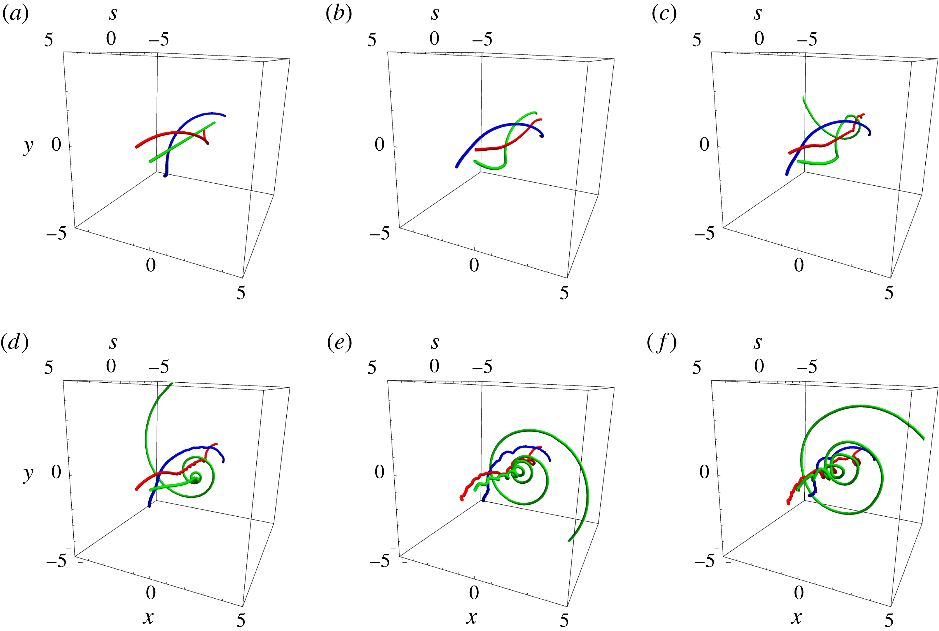
4.2 Travelling wave solutions
To generalise the plane-wave solution dynamics to the case of non-constant amplitudes, we now consider travelling wave solutions that exist for
 $N=2$
satellite vortices around a central vortex. We consider wave coordinates
 $\unicode[STIX]{x1D709}=s-vt$
, for constant
 $v$
, and suppose that
 $\unicode[STIX]{x1D707}_{1}(\unicode[STIX]{x1D709})$
and
 $\unicode[STIX]{x1D707}_{2}(\unicode[STIX]{x1D709})$
have the ansatz
 $$\begin{eqnarray}\unicode[STIX]{x1D707}_{j}(\unicode[STIX]{x1D709})=A_{j}(\unicode[STIX]{x1D709})\exp (\text{i}\unicode[STIX]{x1D703}_{j}(\unicode[STIX]{x1D709})),\end{eqnarray}$$
for
 $A_{j},\unicode[STIX]{x1D703}_{j}\in \mathbb{R}$
and
 $j=\{1,2\}$
.
We transform (4.6) into
 $\unicode[STIX]{x1D709}$
coordinates and substitute (4.13) into the result to obtain, upon taking real and imaginary parts,
 $$\begin{eqnarray}\displaystyle & & \displaystyle \unicode[STIX]{x1D6FC}\unicode[STIX]{x1D6E4}{\displaystyle \frac{\text{d}^{2}A_{1}}{\text{d}\unicode[STIX]{x1D709}^{2}}}+vA_{1}{\displaystyle \frac{\text{d}\unicode[STIX]{x1D703}_{1}}{\text{d}\unicode[STIX]{x1D709}}}-\unicode[STIX]{x1D6FC}\unicode[STIX]{x1D6E4}A_{1}\left({\displaystyle \frac{\text{d}\unicode[STIX]{x1D703}_{1}}{\text{d}\unicode[STIX]{x1D709}}}\right)^{2}+{\displaystyle \frac{4\unicode[STIX]{x1D6E4}}{A_{1}}}\nonumber\\ \displaystyle & & \displaystyle \quad +\,{\displaystyle \frac{2\unicode[STIX]{x1D6E4}}{A_{2}}}\cos (\unicode[STIX]{x1D703}_{2}-\unicode[STIX]{x1D703}_{1})+{\displaystyle \frac{2\unicode[STIX]{x1D6E4}(A_{1}-A_{2}\cos (\unicode[STIX]{x1D703}_{2}-\unicode[STIX]{x1D703}_{1}))}{A_{1}^{2}-2A_{1}A_{2}\cos (\unicode[STIX]{x1D703}_{2}-\unicode[STIX]{x1D703}_{1})+A_{2}^{2}}}=0,\end{eqnarray}$$
 $$\begin{eqnarray}\displaystyle & & \displaystyle \unicode[STIX]{x1D6FC}\unicode[STIX]{x1D6E4}A_{1}{\displaystyle \frac{\text{d}^{2}\unicode[STIX]{x1D703}_{1}}{\text{d}\unicode[STIX]{x1D709}^{2}}}+2\unicode[STIX]{x1D6FC}\unicode[STIX]{x1D6E4}{\displaystyle \frac{\text{d}A_{1}}{\text{d}\unicode[STIX]{x1D709}}}{\displaystyle \frac{\text{d}\unicode[STIX]{x1D703}_{1}}{\text{d}\unicode[STIX]{x1D709}}}-v{\displaystyle \frac{\text{d}A_{1}}{\text{d}\unicode[STIX]{x1D709}}}\nonumber\\ \displaystyle & & \displaystyle \quad +\,{\displaystyle \frac{2\unicode[STIX]{x1D6E4}}{A_{2}}}\sin (\unicode[STIX]{x1D703}_{2}-\unicode[STIX]{x1D703}_{1})+{\displaystyle \frac{2\unicode[STIX]{x1D6E4}A_{2}\sin (\unicode[STIX]{x1D703}_{2}-\unicode[STIX]{x1D703}_{1})}{A_{1}^{2}-2A_{1}A_{2}\cos (\unicode[STIX]{x1D703}_{2}-\unicode[STIX]{x1D703}_{1})+A_{2}^{2}}}=0,\end{eqnarray}$$
 $$\begin{eqnarray}\displaystyle & & \displaystyle \unicode[STIX]{x1D6FC}\unicode[STIX]{x1D6E4}{\displaystyle \frac{\text{d}^{2}A_{2}}{\text{d}\unicode[STIX]{x1D709}^{2}}}+vA_{2}{\displaystyle \frac{\text{d}\unicode[STIX]{x1D703}_{2}}{\text{d}\unicode[STIX]{x1D709}}}-\unicode[STIX]{x1D6FC}\unicode[STIX]{x1D6E4}A_{2}\left({\displaystyle \frac{\text{d}\unicode[STIX]{x1D703}_{2}}{\text{d}\unicode[STIX]{x1D709}}}\right)^{2}+{\displaystyle \frac{4\unicode[STIX]{x1D6E4}}{A_{2}}}\nonumber\\ \displaystyle & & \displaystyle \quad +\,{\displaystyle \frac{2\unicode[STIX]{x1D6E4}}{A_{1}}}\cos (\unicode[STIX]{x1D703}_{1}-\unicode[STIX]{x1D703}_{2})-{\displaystyle \frac{2\unicode[STIX]{x1D6E4}(A_{1}\cos (\unicode[STIX]{x1D703}_{1}-\unicode[STIX]{x1D703}_{2})-A_{2})}{A_{1}^{2}-2A_{1}A_{2}\cos (\unicode[STIX]{x1D703}_{2}-\unicode[STIX]{x1D703}_{1})+A_{2}^{2}}}=0,\end{eqnarray}$$
 $$\begin{eqnarray}\displaystyle & & \displaystyle \unicode[STIX]{x1D6FC}\unicode[STIX]{x1D6E4}A_{2}{\displaystyle \frac{\text{d}^{2}\unicode[STIX]{x1D703}_{2}}{\text{d}\unicode[STIX]{x1D709}^{2}}}+2\unicode[STIX]{x1D6FC}\unicode[STIX]{x1D6E4}{\displaystyle \frac{\text{d}A_{2}}{\text{d}\unicode[STIX]{x1D709}}}{\displaystyle \frac{\text{d}\unicode[STIX]{x1D703}_{2}}{\text{d}\unicode[STIX]{x1D709}}}-v{\displaystyle \frac{\text{d}A_{2}}{\text{d}\unicode[STIX]{x1D709}}}\nonumber\\ \displaystyle & & \displaystyle \quad +\,{\displaystyle \frac{2\unicode[STIX]{x1D6E4}}{A_{1}}}\sin (\unicode[STIX]{x1D703}_{1}-\unicode[STIX]{x1D703}_{2})-{\displaystyle \frac{2\unicode[STIX]{x1D6E4}A_{1}\sin (\unicode[STIX]{x1D703}_{1}-\unicode[STIX]{x1D703}_{2})}{A_{1}^{2}-2A_{1}A_{2}\cos (\unicode[STIX]{x1D703}_{2}-\unicode[STIX]{x1D703}_{1})+A_{2}^{2}}}=0.\end{eqnarray}$$
We numerically solve (4.14)–(4.17) for the initial conditions
 $A_{1}(\unicode[STIX]{x1D709}=0)=0.5$
,
 $A_{1}^{\prime }(\unicode[STIX]{x1D709}=0)=0$
,
 $\unicode[STIX]{x1D703}_{1}(\unicode[STIX]{x1D709}=0)=0$
,
 $\unicode[STIX]{x1D703}_{1}^{\prime }(\unicode[STIX]{x1D709}=0)=1$
,
 $A_{2}(\unicode[STIX]{x1D709}=0)=0.5$
,
 $A_{2}^{\prime }(\unicode[STIX]{x1D709}=0)=0$
,
 $\unicode[STIX]{x1D703}_{2}(\unicode[STIX]{x1D709}=0)=\unicode[STIX]{x03C0}$
and
 $\unicode[STIX]{x1D703}_{2}^{\prime }(\unicode[STIX]{x1D709}=0)=1.1$
with
 $v=1$
in figure 25 and show the corresponding filament shapes in figure 26 for
 $\unicode[STIX]{x1D708}(t,s)=0$
,
 $\unicode[STIX]{x1D6FC}=\unicode[STIX]{x1D6E4}=1$
and times
 $t=\{0,2,4,6\}$
. We observe that the resulting solutions are chaotic in nature, exhibiting aperiodicity and a hypersensitivity to the initial conditions imposed.
plots of
 $A_{j}(\unicode[STIX]{x1D709})$
and the real and imaginary components of
 $\exp (\text{i}\unicode[STIX]{x1D703}_{j}(\unicode[STIX]{x1D709}))$
(shown in black and red respectively) calculated by the numerical solution of (4.14)–(4.17) for
 $j=\{1,2\}$
. The initial conditions are
 $A_{1}(\unicode[STIX]{x1D709}=0)=0.5$
,
 $A_{1}^{\prime }(\unicode[STIX]{x1D709}=0)=0$
,
 $\unicode[STIX]{x1D703}_{1}(\unicode[STIX]{x1D709}=0)=0$
,
 $\unicode[STIX]{x1D703}_{1}^{\prime }(\unicode[STIX]{x1D709}=0)=1$
,
 $A_{2}(\unicode[STIX]{x1D709}=0)=0.5$
,
 $A_{2}^{\prime }(\unicode[STIX]{x1D709}=0)=0$
,
 $\unicode[STIX]{x1D703}_{2}(\unicode[STIX]{x1D709}=0)=\unicode[STIX]{x03C0}$
and
 $\unicode[STIX]{x1D703}_{2}^{\prime }(\unicode[STIX]{x1D709}=0)=1.1$
with
 $v=1$
.
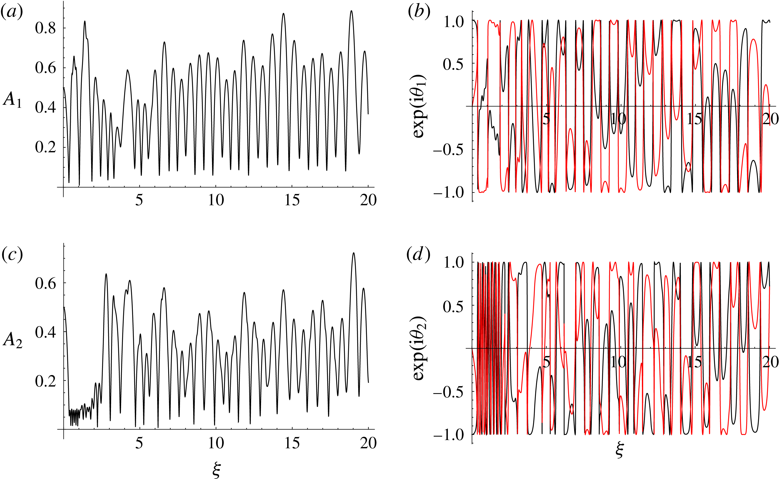
Time evolution of travelling wave solutions in a co-rotating vortex hierarchy featuring two satellite vortices orbiting around a central filament. Plots of
 $\unicode[STIX]{x1D713}_{0}(t,s)$
,
 $\unicode[STIX]{x1D713}_{1}(t,s)$
and
 $\unicode[STIX]{x1D713}_{2}(t,s)$
(shown in blue, red and green respectively) were obtained by solving (4.14)–(4.17) with
 $\unicode[STIX]{x1D708}(t,s)=0$
for the initial conditions
 $A_{1}(\unicode[STIX]{x1D709}=0)=0.5$
,
 $A_{1}^{\prime }(\unicode[STIX]{x1D709}=0)=0$
,
 $\unicode[STIX]{x1D703}_{1}(\unicode[STIX]{x1D709}=0)=0$
,
 $\unicode[STIX]{x1D703}_{1}^{\prime }(\unicode[STIX]{x1D709}=0)=1$
,
 $A_{2}(\unicode[STIX]{x1D709}=0)=0.5$
,
 $A_{2}^{\prime }(\unicode[STIX]{x1D709}=0)=0$
,
 $\unicode[STIX]{x1D703}_{2}(\unicode[STIX]{x1D709}=0)=\unicode[STIX]{x03C0}$
and
 $\unicode[STIX]{x1D703}_{2}^{\prime }(\unicode[STIX]{x1D709}=0)=1.1$
with
 $v=\unicode[STIX]{x1D6FC}=\unicode[STIX]{x1D6E4}=1$
. Times (a)
 $t=0$
, (b)
 $t=2$
, (c)
 $t=4$
and (d)
 $t=6$
are shown over the arclength
 $s\in [0,5]$
.
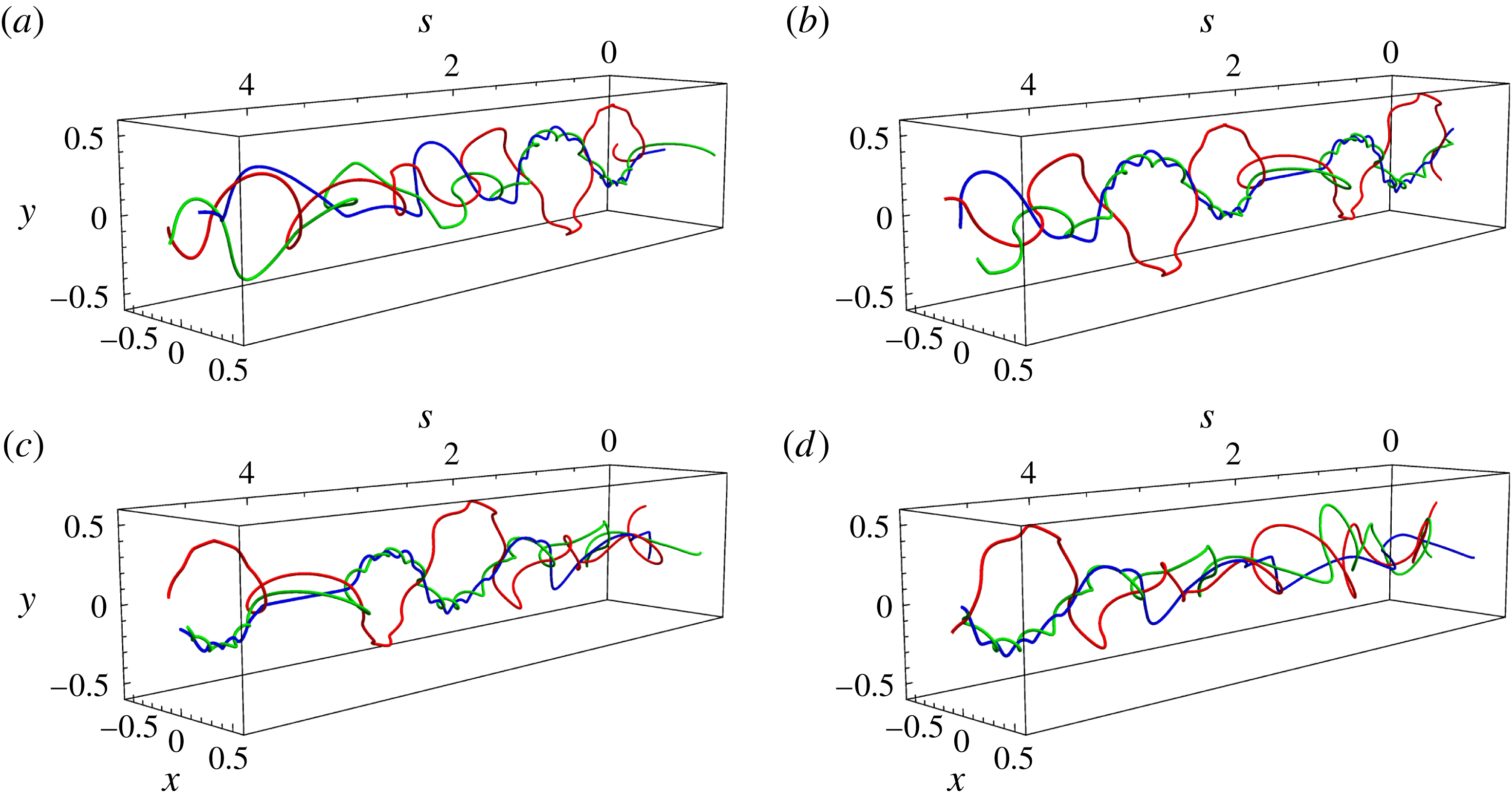
4.3 Self-similar solutions
We study solutions for
 $N=2$
satellite vortices around a central filament of the form
 $\unicode[STIX]{x1D707}_{j}(t,s)=s\unicode[STIX]{x1D712}_{j}(\unicode[STIX]{x1D702})$
, for
 $\unicode[STIX]{x1D702}=s/\sqrt{t}$
and
 $j=\{1,2\}$
. By using the amplitude–phase ansatz
 $$\begin{eqnarray}\unicode[STIX]{x1D712}_{j}(\unicode[STIX]{x1D702})=A_{j}(\unicode[STIX]{x1D702})\exp (\text{i}\unicode[STIX]{x1D703}_{j}(\unicode[STIX]{x1D702})),\end{eqnarray}$$
with
 $A_{j},\unicode[STIX]{x1D703}_{j}\in \mathbb{R}$
, we transform (4.6) and take real and imaginary parts to obtain
 $$\begin{eqnarray}\displaystyle & & \displaystyle \unicode[STIX]{x1D6FC}\unicode[STIX]{x1D6E4}\unicode[STIX]{x1D702}^{2}{\displaystyle \frac{\text{d}^{2}A_{1}}{\text{d}\unicode[STIX]{x1D702}^{2}}}-\unicode[STIX]{x1D6FC}\unicode[STIX]{x1D6E4}\unicode[STIX]{x1D702}^{2}A_{1}\left({\displaystyle \frac{\text{d}\unicode[STIX]{x1D703}_{1}}{\text{d}\unicode[STIX]{x1D702}}}\right)^{2}+2\unicode[STIX]{x1D702}{\displaystyle \frac{\text{d}A_{1}}{\text{d}\unicode[STIX]{x1D702}}}+{\displaystyle \frac{\unicode[STIX]{x1D702}^{3}}{2}}A_{1}{\displaystyle \frac{\text{d}\unicode[STIX]{x1D703}_{1}}{\text{d}\unicode[STIX]{x1D702}}}+{\displaystyle \frac{4\unicode[STIX]{x1D6E4}}{A_{1}}}\nonumber\\ \displaystyle & & \displaystyle \quad +\,{\displaystyle \frac{2\unicode[STIX]{x1D6E4}}{A_{2}}}\cos (\unicode[STIX]{x1D703}_{2}-\unicode[STIX]{x1D703}_{1})+{\displaystyle \frac{2\unicode[STIX]{x1D6E4}(A_{1}-A_{2}\cos (\unicode[STIX]{x1D703}_{2}-\unicode[STIX]{x1D703}_{1}))}{A_{1}^{2}-2A_{1}A_{2}\cos (\unicode[STIX]{x1D703}_{2}-\unicode[STIX]{x1D703}_{1})+A_{2}^{2}}}=0,\end{eqnarray}$$
 $$\begin{eqnarray}\displaystyle & & \displaystyle \unicode[STIX]{x1D6FC}\unicode[STIX]{x1D6E4}\unicode[STIX]{x1D702}^{2}A_{1}{\displaystyle \frac{\text{d}^{2}\unicode[STIX]{x1D703}_{1}}{\text{d}\unicode[STIX]{x1D702}^{2}}}+2\unicode[STIX]{x1D6FC}\unicode[STIX]{x1D702}^{2}\unicode[STIX]{x1D6E4}{\displaystyle \frac{\text{d}A_{1}}{\text{d}\unicode[STIX]{x1D702}}}{\displaystyle \frac{\text{d}\unicode[STIX]{x1D703}_{1}}{\text{d}\unicode[STIX]{x1D702}}}+2\unicode[STIX]{x1D702}A_{1}{\displaystyle \frac{\text{d}\unicode[STIX]{x1D703}_{1}}{\text{d}\unicode[STIX]{x1D702}}}-{\displaystyle \frac{\unicode[STIX]{x1D702}^{3}}{2}}{\displaystyle \frac{\text{d}A_{1}}{\text{d}\unicode[STIX]{x1D702}}}\nonumber\\ \displaystyle & & \displaystyle \quad +\,{\displaystyle \frac{2\unicode[STIX]{x1D6E4}}{A_{2}}}\sin (\unicode[STIX]{x1D703}_{2}-\unicode[STIX]{x1D703}_{1})+{\displaystyle \frac{2\unicode[STIX]{x1D6E4}A_{2}\sin (\unicode[STIX]{x1D703}_{2}-\unicode[STIX]{x1D703}_{1})}{A_{1}^{2}-2A_{1}A_{2}\cos (\unicode[STIX]{x1D703}_{2}-\unicode[STIX]{x1D703}_{1})+A_{2}^{2}}}=0,\end{eqnarray}$$
 $$\begin{eqnarray}\displaystyle & & \displaystyle \unicode[STIX]{x1D6FC}\unicode[STIX]{x1D6E4}\unicode[STIX]{x1D702}^{2}{\displaystyle \frac{\text{d}^{2}A_{2}}{\text{d}\unicode[STIX]{x1D702}^{2}}}-\unicode[STIX]{x1D6FC}\unicode[STIX]{x1D6E4}\unicode[STIX]{x1D702}^{2}A_{2}\left({\displaystyle \frac{\text{d}\unicode[STIX]{x1D703}_{2}}{\text{d}\unicode[STIX]{x1D702}}}\right)^{2}+2\unicode[STIX]{x1D702}{\displaystyle \frac{\text{d}A_{2}}{\text{d}\unicode[STIX]{x1D702}}}+{\displaystyle \frac{\unicode[STIX]{x1D702}^{3}}{2}}A_{2}{\displaystyle \frac{\text{d}\unicode[STIX]{x1D703}_{2}}{\text{d}\unicode[STIX]{x1D702}}}+{\displaystyle \frac{4\unicode[STIX]{x1D6E4}}{A_{2}}}\nonumber\\ \displaystyle & & \displaystyle \quad +\,{\displaystyle \frac{2\unicode[STIX]{x1D6E4}}{A_{1}}}\cos (\unicode[STIX]{x1D703}_{1}-\unicode[STIX]{x1D703}_{2})-{\displaystyle \frac{2\unicode[STIX]{x1D6E4}(A_{1}\cos (\unicode[STIX]{x1D703}_{1}-\unicode[STIX]{x1D703}_{2})-A_{2})}{A_{1}^{2}-2A_{1}A_{2}\cos (\unicode[STIX]{x1D703}_{2}-\unicode[STIX]{x1D703}_{1})+A_{2}^{2}}}=0,\end{eqnarray}$$
 $$\begin{eqnarray}\displaystyle & & \displaystyle \unicode[STIX]{x1D6FC}\unicode[STIX]{x1D6E4}\unicode[STIX]{x1D702}^{2}A_{2}{\displaystyle \frac{\text{d}^{2}\unicode[STIX]{x1D703}_{2}}{\text{d}\unicode[STIX]{x1D702}^{2}}}+2\unicode[STIX]{x1D6FC}\unicode[STIX]{x1D702}^{2}\unicode[STIX]{x1D6E4}{\displaystyle \frac{\text{d}A_{2}}{\text{d}\unicode[STIX]{x1D702}}}{\displaystyle \frac{\text{d}\unicode[STIX]{x1D703}_{2}}{\text{d}\unicode[STIX]{x1D702}}}+2\unicode[STIX]{x1D702}A_{2}{\displaystyle \frac{\text{d}\unicode[STIX]{x1D703}_{2}}{\text{d}\unicode[STIX]{x1D702}}}-{\displaystyle \frac{\unicode[STIX]{x1D702}^{3}}{2}}{\displaystyle \frac{\text{d}A_{2}}{\text{d}\unicode[STIX]{x1D702}}}\nonumber\\ \displaystyle & & \displaystyle \quad +\,{\displaystyle \frac{2\unicode[STIX]{x1D6E4}}{A_{1}}}\sin (\unicode[STIX]{x1D703}_{1}-\unicode[STIX]{x1D703}_{2})-{\displaystyle \frac{2\unicode[STIX]{x1D6E4}A_{1}\sin (\unicode[STIX]{x1D703}_{1}-\unicode[STIX]{x1D703}_{2})}{A_{1}^{2}-2A_{1}A_{2}\cos (\unicode[STIX]{x1D703}_{2}-\unicode[STIX]{x1D703}_{1})+A_{2}^{2}}}=0.\end{eqnarray}$$
We numerically solve (4.19)–(4.22) for the initial conditions
 $A_{1}(\unicode[STIX]{x1D702}=0.01)=1$
,
 $A_{1}^{\prime }(\unicode[STIX]{x1D702}=0.01)=0$
,
 $\unicode[STIX]{x1D703}_{1}(\unicode[STIX]{x1D702}=0.01)=0$
,
 $\unicode[STIX]{x1D703}_{1}^{\prime }(\unicode[STIX]{x1D702}=0.01)=0.5$
,
 $A_{2}(\unicode[STIX]{x1D702}=0.01)=1$
,
 $A_{2}^{\prime }(\unicode[STIX]{x1D702}=0.01)=0$
,
 $\unicode[STIX]{x1D703}_{2}(\unicode[STIX]{x1D702}=0.01)=\unicode[STIX]{x03C0}$
and
 $\unicode[STIX]{x1D703}_{2}^{\prime }(\unicode[STIX]{x1D702}=0.01)=0.6$
and plot the results in figure 27. Furthermore, we illustrate the corresponding vortex filament shapes with
 $\unicode[STIX]{x1D708}(t,s)=0$
and
 $\unicode[STIX]{x1D6FC}=\unicode[STIX]{x1D6E4}=1$
in figure 28 for times
 $t=\{0.05,0.5,5,50,500,5000\}$
. Again, the vortex filament interactions appear to yield chaotic dynamics. Additionally, the filament pair with the larger initial twist
 $\unicode[STIX]{x1D703}^{\prime }(\unicode[STIX]{x1D709})$
, in the present case
 $\unicode[STIX]{x1D713}_{0}(t,s)$
and
 $\unicode[STIX]{x1D713}_{2}(t,s)$
, tightly intertwine and form a macroscopic filament that interacts with the other satellite vortex.
Plots of
 $A_{j}(\unicode[STIX]{x1D702})$
and the real and imaginary components of
 $\exp (\text{i}\unicode[STIX]{x1D703}_{j}(\unicode[STIX]{x1D702}))$
(shown in black and red respectively) calculated by the numerical solution of (4.19)–(4.22) for
 $j=\{1,2\}$
. The initial conditions are
 $A_{1}(\unicode[STIX]{x1D702}=0.01)=1$
,
 $A_{1}^{\prime }(\unicode[STIX]{x1D702}=0.01)=0$
,
 $\unicode[STIX]{x1D703}_{1}(\unicode[STIX]{x1D702}=0.01)=0$
,
 $\unicode[STIX]{x1D703}_{1}^{\prime }(\unicode[STIX]{x1D702}=0.01)=0.5$
,
 $A_{2}(\unicode[STIX]{x1D702}=0.01)=1$
,
 $A_{2}^{\prime }(\unicode[STIX]{x1D702}=0.01)=0$
,
 $\unicode[STIX]{x1D703}_{2}(\unicode[STIX]{x1D702}=0.01)=\unicode[STIX]{x03C0}$
and
 $\unicode[STIX]{x1D703}_{2}^{\prime }(\unicode[STIX]{x1D702}=0.01)=0.6$
.
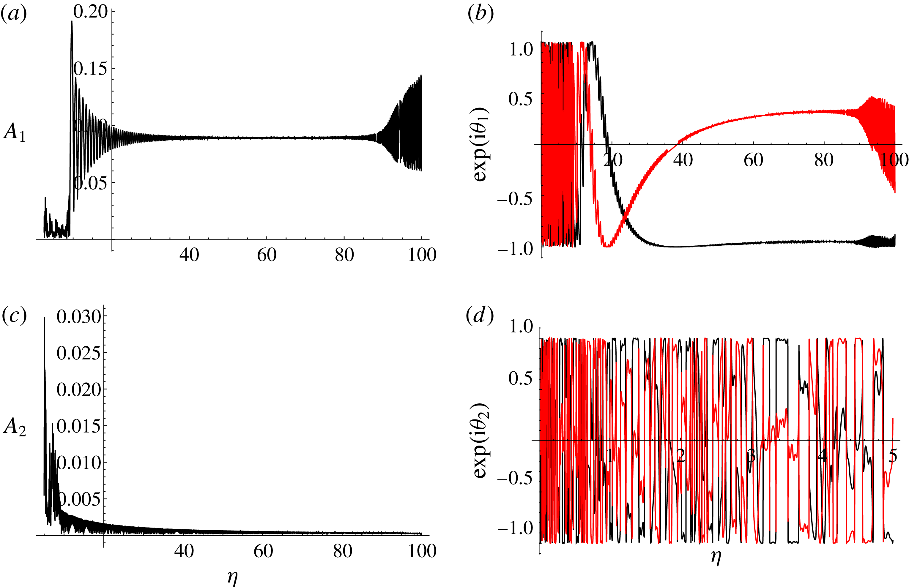
Time evolution of self-similar solutions in a co-rotating vortex hierarchy featuring two satellite vortices orbiting around a central filament. Plots of
 $\unicode[STIX]{x1D713}_{0}(t,s)$
,
 $\unicode[STIX]{x1D713}_{1}(t,s)$
and
 $\unicode[STIX]{x1D713}_{2}(t,s)$
(shown in blue, red and green respectively) were obtained by solving (4.19)–(4.22) with
 $\unicode[STIX]{x1D708}(t,s)=0$
for the initial conditions
 $A_{1}(\unicode[STIX]{x1D702}=0.01)=1$
,
 $A_{1}^{\prime }(\unicode[STIX]{x1D702}=0.01)=0$
,
 $\unicode[STIX]{x1D703}_{1}(\unicode[STIX]{x1D702}=0.01)=0$
,
 $\unicode[STIX]{x1D703}_{1}^{\prime }(\unicode[STIX]{x1D702}=0.01)=0.5$
,
 $A_{2}(\unicode[STIX]{x1D702}=0.01)=1$
,
 $A_{2}^{\prime }(\unicode[STIX]{x1D702}=0.01)=0$
,
 $\unicode[STIX]{x1D703}_{2}(\unicode[STIX]{x1D702}=0.01)=\unicode[STIX]{x03C0}$
and
 $\unicode[STIX]{x1D703}_{2}^{\prime }(\unicode[STIX]{x1D702}=0.01)=0.6$
, with
 $\unicode[STIX]{x1D6FC}=\unicode[STIX]{x1D6E4}=1$
. Times (a)
 $t=0.05$
, (b)
 $t=0.5$
, (c)
 $t=5$
, (d)
 $t=50$
, (e)
 $t=500$
and (f)
 $t=5000$
are shown over the arclength
 $s\in [2,10]$
.
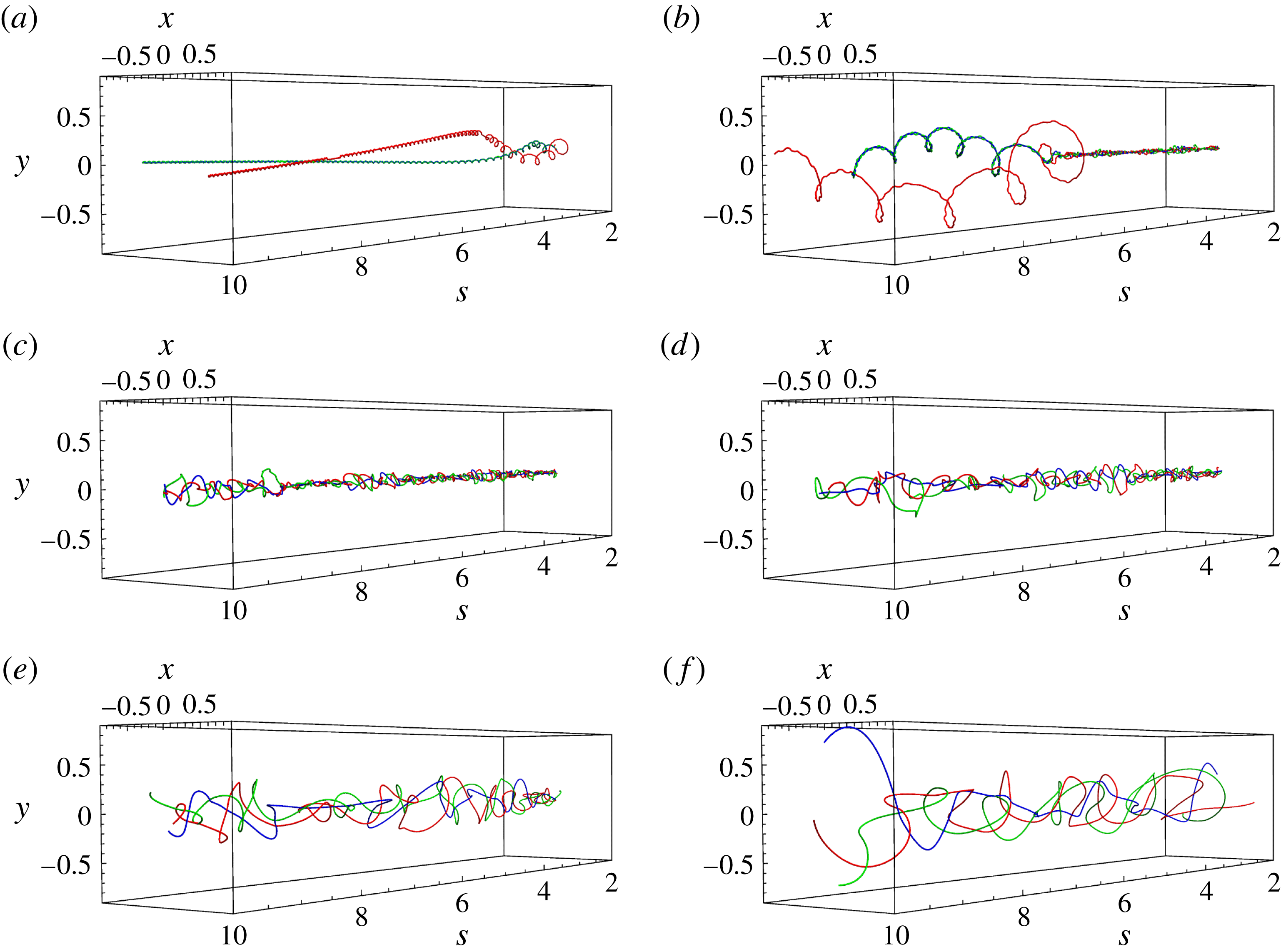
5 Discussion
When studying the co-rotating vortices with large separation between the filaments, we found self-similar solutions that exhibited a conical-helix-like structure (conical-type solutions have previously been seen for isolated vortex filaments (Van Gorder Reference Van Gorder2016)) and also travelling wave solutions. For this case, the vortex pair repelled in opposite directions. In the self-similar case, the rotation of the vortex helices was such that they rotated in the same direction, with the orientation of one helix being a reflection of the other. In figure 4, both vortices have circulation
 $\unicode[STIX]{x1D6E4}>0$
; however, the helices rotate in a clockwise direction, with the direction of a helix rotation being opposite to an individual filament circulation.
In the case of counter-rotating filaments with large separation between the filaments, we found that the position of the vortex pair centre and the deviations from this centre were strongly coupled, unlike what was shown for the co-rotating vortex filaments, where these two terms decoupled. This somewhat complicates the solution procedure. For the counter-rotating travelling wave solutions with large separation between the filaments, there was no secular vortex repulsion or attraction, contrary to what was previously seen with the co-rotating pair; rather, deviations of the vortex pair had a constant offset, which was determined by the speed of the travelling wave. The centre of the vortex pair will move from its initial position over time; that is to say, the filaments will move together at a constant velocity through the 3D flow. Furthermore, we found that the wave speed of the travelling wave could stabilise the vortex pair so that they remained together. There was an additional effect that was not predicted by the 2D theory, namely oscillations in the deviations of the two filaments from the centre. These vibrations caused the amplitude of the helices to periodically vary in a manner such that the individual helices were out of phase with each other. We observed that as time evolved, the filament initially had a helical shape (figure 6 a), whose amplitude shrunk (figure 6 b), before returning to its original shape (figure 6 c). The other helix grew in amplitude as the first filament decreased. Meanwhile, for the counter-rotating self-similar solutions with large separation between the filaments, we found that the helices rotated in the opposite direction to the respective circulation of the vortex, as was also seen in the co-rotating case.
Regarding travelling wave solutions for intertwined vortex filaments in the co-rotating case, as the filaments approached each other, their attraction occurred on a very fast time scale, for
 $\unicode[STIX]{x1D6FE}\ll 1$
, until the pair reached their minimum separation, at which point they repelled one another. The orientation of the vortices at this moment changed almost instantaneously, as
 $\unicode[STIX]{x1D6FE}\tan ^{-1}(c_{1}c_{2}+c_{1}\unicode[STIX]{x1D709}/\unicode[STIX]{x1D6FE}^{2n-1})$
dominated in the expression (3.16). As the filaments separated, with their amplitudes
 $A\rightarrow O(1)$
, the time scale slowed down and the orientation of the pair evolved according to the
 $v\unicode[STIX]{x1D709}/2$
term, which now dominated in (B 6). The filaments then reached their maximum separation before attracting each other again and repeating the cycle.
For the intertwined rotating planar filaments in the co-rotating case, we observed a couple of behaviours, depending on the parameter value
 $\unicode[STIX]{x1D714}$
. When
 $\unicode[STIX]{x1D714}>0$
,
 $A\rightarrow 0^{+}$
as
 $s\rightarrow \pm \infty$
, and the vortex pair was found to collapse if the respective circulations of the filaments were in the same direction as the pair rotated in. On the other hand, if
 $\unicode[STIX]{x1D714}<0$
, then
 $A\rightarrow \infty$
as
 $s\rightarrow \infty$
. Considering a vortex pair with circulations in the opposite direction, rotating pairs with
 $\unicode[STIX]{x1D714}<0$
would also collapse or, if
 $\unicode[STIX]{x1D714}>0$
, might also repel without bound. The strong dependence of solutions on the sign of the spectral parameter
 $\unicode[STIX]{x1D714}$
was previously discussed for single isolated planar vortex filaments under the LIA (Van Gorder Reference Van Gorder2013c
) and Biot–Savart (Van Gorder Reference Van Gorder2015b
) dynamics.
When intertwined self-similar filament structures in the co-rotating case came into close proximity, the orientation of separation changed rapidly. In the large-time limit
 $t\rightarrow \infty$
, the amplitude and wavelength of the filament separation function became larger and variations in the orientation became slower. As
 $t\rightarrow \infty$
, the separation of the filaments themselves grew to infinity, and their orientation became planar along a single direction. This smoothing out of an originally rapidly varying filament was exactly seen even in models of isolated self-similar filaments (see Van Gorder (Reference Van Gorder2016) and references therein).
For travelling wave solutions to the counter-rotating intertwined filaments, some differences existed compared with the co-rotating case. If
 $\unicode[STIX]{x1D6FE}=0$
, then the orientation of the counter-rotating pair did not change and the oscillation remained completely planar for all time, with the pair no longer collapsing as
 $t\rightarrow \infty$
. For any value of
 $v$
(the wave speed) or
 $\unicode[STIX]{x1D6FE}$
, the counter-rotating vortices would not meet. If the velocity of the travelling waves was
 $v=0$
, corresponding to standing or stationary waves, the filament pair repelled. If the wave speed
 $v$
was non-zero, then periodic solutions in the wave amplitude were found for all values of
 $\unicode[STIX]{x1D6FE}$
. As such, the counter-rotating vortex filaments had a different asymptotic structure that no longer depended on
 $\unicode[STIX]{x1D6FE}$
, in contrast to what was found for the corresponding co-rotating travelling wave solutions.
For the counter-rotating intertwined planar vortex filaments, we imposed boundary conditions so that the quantity denoting the separation of the vortex filament pair was oscillatory along the arclength parameter. The filament shapes were therefore asymmetric when compared with the symmetrical co-rotating filaments, a direct result of the coupling of the position of the vortex pair centre and the deviations from this centre. In contrast to the self-similar solutions in earlier sections, the self-similar intertwined counter-rotating filaments were never in very close proximity, so that the orientation of the pair did not rapidly change according to the dependence of
 $1/A$
in (3.44). The vortex pair remained separated, but as
 $t\rightarrow \infty$
, the centre of the vortex pair moved such that the filaments began to intertwine and rotate around each other.
All of the above conclusions correspond to two mutually interacting vortex filaments. To extend these results, we considered the co-rotating vortex hierarchy with satellite vortex filaments surrounding a central vortex. In the case in which all vortex filaments had plane-wave structure, the angular velocity of the vortex configuration depended on the wavenumber,
 $k$
, the distance of the satellite filaments from the central filament,
 $B$
, and the number of satellite filaments,
 $N$
. In our numerical simulations, the central filament exhibited an instability, which grew and spiralled inwards through the hierarchy. In response, small-wavelength perturbations developed in the satellite filaments, and these then grew without bound, leading to eventual collapse of the structure.
For the more general travelling wave case, numerical simulations for the co-rotating vortex hierarchy allowed us to find solutions that appeared to be chaotic in nature, exhibiting aperiodicity and a strong sensitivity to the initial conditions imposed. In the case of self-similar vortex filament structures arranged in this hierarchy, we again observed what appeared to be chaotic dynamics as the system evolved in time away from the initial configuration, and, furthermore, the filament pair with the larger initial twist tightly intertwined to form a macroscopic filament that interacted with the other vortex. Such results are interesting, as they show that chaotic dynamics are possible in configurations with relatively small numbers of vortex filaments. Chaos, either deterministic (Nemirovskii & Baltsevich Reference Nemirovskii and Baltsevich2001) or stochastic (Nemirovskii Reference Nemirovskii2008), has previously been discussed in relation to quantum turbulence. Chaotic dynamics from Kelvin waves along quantised vortex filaments (corresponding to plane-wave solutions, or generalisations such as the travelling wave solutions we have considered) carrying energy to small scales and leading to a cascade has been suggested (Nemirovskii Reference Nemirovskii2013) as one route for the transition to turbulence in superfluid helium. This direction is particularly promising in light of the fact that Kelvin waves have recently been observed experimentally in superfluid helium (Fonda et al. Reference Fonda, Meichle, Ouellette, Hormoz and Lathrop2014).
Appendix A. Asymptotic solutions of vortex pair configurations
A.1 Asymptotic solutions for § 2.1.1
A.1.1 Fast wave-scale dynamics
We define a small parameter
 $\unicode[STIX]{x1D716}=1/d\ll 1$
and expand the nonlinear interaction terms in (2.7) to give
 $$\begin{eqnarray}{\displaystyle \frac{\text{d}^{2}\unicode[STIX]{x1D707}}{\text{d}\unicode[STIX]{x1D709}^{2}}}-\text{i}v{\displaystyle \frac{\text{d}\unicode[STIX]{x1D707}}{\text{d}\unicode[STIX]{x1D709}}}+4\mathop{\sum }_{n=0}^{\infty }(-1)^{n}\unicode[STIX]{x1D716}^{n+1}(\unicode[STIX]{x1D707}^{\ast })^{n}=0,\end{eqnarray}$$
where
 $(~)^{\ast }$
is the complex conjugate of the variable.
We make use of the fact that we are studying large separation distances and expand
 $\unicode[STIX]{x1D707}(\unicode[STIX]{x1D709})$
as a series in
 $\unicode[STIX]{x1D716}$
. In particular,
 $\unicode[STIX]{x1D707}=\sum _{m=0}^{\infty }\unicode[STIX]{x1D716}^{m}\unicode[STIX]{x1D707}^{(m)}$
, so that, for increasing orders of
 $\unicode[STIX]{x1D716}$
,
 $$\begin{eqnarray}\displaystyle & \displaystyle O(\unicode[STIX]{x1D716}^{0}):\quad 0={\displaystyle \frac{\text{d}^{2}\unicode[STIX]{x1D707}^{(0)}}{\text{d}\unicode[STIX]{x1D709}^{2}}}-\text{i}v{\displaystyle \frac{\text{d}\unicode[STIX]{x1D707}^{(0)}}{\text{d}\unicode[STIX]{x1D709}}}, & \displaystyle\end{eqnarray}$$
 $$\begin{eqnarray}\displaystyle & \displaystyle O(\unicode[STIX]{x1D716}^{1}):\quad 0={\displaystyle \frac{\text{d}^{2}\unicode[STIX]{x1D707}^{(1)}}{\text{d}\unicode[STIX]{x1D709}^{2}}}-\text{i}v{\displaystyle \frac{\text{d}\unicode[STIX]{x1D707}^{(1)}}{\text{d}\unicode[STIX]{x1D709}}}+4, & \displaystyle\end{eqnarray}$$
 $$\begin{eqnarray}\displaystyle & \displaystyle O(\unicode[STIX]{x1D716}^{2}):\quad 0={\displaystyle \frac{\text{d}^{2}\unicode[STIX]{x1D707}^{(2)}}{\text{d}\unicode[STIX]{x1D709}^{2}}}-\text{i}v{\displaystyle \frac{\text{d}\unicode[STIX]{x1D707}^{(2)}}{\text{d}\unicode[STIX]{x1D709}}}-4(\unicode[STIX]{x1D707}^{(0)})^{\ast }, & \displaystyle\end{eqnarray}$$
the exact solutions of which give the second-order asymptotic solution (2.8).
A.1.2 Slow wave-scale dynamics
Let
 $\unicode[STIX]{x1D716}=1/d\ll 1$
. We note that
 $\unicode[STIX]{x1D6FD}=2$
in (2.9) from balancing the vortex interaction term in (A 1). However, in order for
 $\unicode[STIX]{x1D703}(\unicode[STIX]{x1D709})$
to satisfy initial conditions on
 $\unicode[STIX]{x1D707}(\unicode[STIX]{x1D709})$
, the perturbation expansion must begin at
 $O(\unicode[STIX]{x1D716}^{-1})$
. Therefore, we set
 $\unicode[STIX]{x1D703}(\unicode[STIX]{x1D709})=\sum _{n=0}^{\infty }\unicode[STIX]{x1D716}^{n-1}\unicode[STIX]{x1D703}^{(n)}(\unicode[STIX]{x1D709})$
, which gives, upon extracting orders of
 $\unicode[STIX]{x1D716}$
,
 $$\begin{eqnarray}\displaystyle & \displaystyle O(\unicode[STIX]{x1D716}^{0}):\quad 0=\text{i}{\displaystyle \frac{\text{d}^{2}\unicode[STIX]{x1D703}^{(0)}}{\text{d}\unicode[STIX]{x1D709}^{2}}}+v{\displaystyle \frac{\text{d}\unicode[STIX]{x1D703}^{(0)}}{\text{d}\unicode[STIX]{x1D709}}}, & \displaystyle\end{eqnarray}$$
 $$\begin{eqnarray}\displaystyle & \displaystyle O(\unicode[STIX]{x1D716}^{1}):\quad 0=\text{i}{\displaystyle \frac{\text{d}^{2}\unicode[STIX]{x1D703}^{(1)}}{\text{d}\unicode[STIX]{x1D709}^{2}}}-\left({\displaystyle \frac{\text{d}\unicode[STIX]{x1D703}^{(0)}}{\text{d}\unicode[STIX]{x1D709}}}\right)^{2}+v{\displaystyle \frac{\text{d}\unicode[STIX]{x1D703}^{(1)}}{\text{d}\unicode[STIX]{x1D709}}}+4, & \displaystyle\end{eqnarray}$$
 $$\begin{eqnarray}\displaystyle & \displaystyle O(\unicode[STIX]{x1D716}^{2}):\quad 0=\text{i}{\displaystyle \frac{\text{d}^{2}\unicode[STIX]{x1D703}^{(2)}}{\text{d}\unicode[STIX]{x1D709}^{2}}}-2{\displaystyle \frac{\text{d}\unicode[STIX]{x1D703}^{(0)}}{\text{d}\unicode[STIX]{x1D709}}}{\displaystyle \frac{\text{d}\unicode[STIX]{x1D703}^{(1)}}{\text{d}\unicode[STIX]{x1D709}}}+v{\displaystyle \frac{\text{d}\unicode[STIX]{x1D703}^{(2)}}{\text{d}\unicode[STIX]{x1D709}}}, & \displaystyle\end{eqnarray}$$
the solution of which results in the slow wave-scale solution (2.10).
A.2 Asymptotic solutions for § 2.1.2
Making use of the fact that
 $\unicode[STIX]{x1D716}=d^{-1}\ll 1$
, we expand the nonlinear interaction term in (2.11) as a power series to obtain
 $$\begin{eqnarray}{\displaystyle \frac{\text{d}^{2}\unicode[STIX]{x1D712}}{\text{d}\unicode[STIX]{x1D702}^{2}}}-{\displaystyle \frac{\text{i}\unicode[STIX]{x1D702}}{2}}{\displaystyle \frac{\text{d}\unicode[STIX]{x1D712}}{\text{d}\unicode[STIX]{x1D702}}}+{\displaystyle \frac{\text{i}}{2}}\unicode[STIX]{x1D712}+4\mathop{\sum }_{n=0}^{\infty }(-1)^{n}\unicode[STIX]{x1D716}^{n+1}(\unicode[STIX]{x1D712}^{\ast })^{n}=0,\end{eqnarray}$$
and further expand
 $\unicode[STIX]{x1D712}(\unicode[STIX]{x1D702})$
as a power series in
 $\unicode[STIX]{x1D716}$
, so that
 $\unicode[STIX]{x1D712}(\unicode[STIX]{x1D702})=\sum _{n=0}^{\infty }\unicode[STIX]{x1D716}^{n}\unicode[STIX]{x1D712}^{(n)}$
, to find
 $$\begin{eqnarray}\displaystyle & \displaystyle O(\unicode[STIX]{x1D716}^{0}):\quad 0={\displaystyle \frac{\text{d}^{2}\unicode[STIX]{x1D712}^{(0)}}{\text{d}\unicode[STIX]{x1D702}^{2}}}-{\displaystyle \frac{\text{i}\unicode[STIX]{x1D702}}{2}}{\displaystyle \frac{\text{d}\unicode[STIX]{x1D712}^{(0)}}{\text{d}\unicode[STIX]{x1D702}}}+{\displaystyle \frac{\text{i}}{2}}\unicode[STIX]{x1D712}^{(0)}, & \displaystyle\end{eqnarray}$$
 $$\begin{eqnarray}\displaystyle & \displaystyle O(\unicode[STIX]{x1D716}^{1}):\quad 0={\displaystyle \frac{\text{d}^{2}\unicode[STIX]{x1D712}^{(1)}}{\text{d}\unicode[STIX]{x1D702}^{2}}}-{\displaystyle \frac{\text{i}\unicode[STIX]{x1D702}}{2}}{\displaystyle \frac{\text{d}\unicode[STIX]{x1D712}^{(1)}}{\text{d}\unicode[STIX]{x1D702}}}+{\displaystyle \frac{\text{i}}{2}}\unicode[STIX]{x1D712}^{(1)}+4, & \displaystyle\end{eqnarray}$$
the solution of which gives the first-order asymptotic expansion in (2.12).
A.3 Section 2.2.1
A.3.1 Fast wave-scale dynamics
We expand the interaction term in (2.18) as a series in
 $\unicode[STIX]{x1D716}=1/d\ll 1$
to obtain
 $$\begin{eqnarray}{\displaystyle \frac{\text{d}^{2}\unicode[STIX]{x1D707}}{\text{d}\unicode[STIX]{x1D709}^{2}}}+v^{2}\unicode[STIX]{x1D707}-4\mathop{\sum }_{n=0}^{\infty }(-1)^{n}\unicode[STIX]{x1D716}^{n+1}(\unicode[STIX]{x1D707}^{\ast })^{n}=\unicode[STIX]{x1D6FF},\end{eqnarray}$$
and split
 $\unicode[STIX]{x1D707}(t,s)$
into real and imaginary components, so that
 $\unicode[STIX]{x1D707}(\unicode[STIX]{x1D709})=X(\unicode[STIX]{x1D709})+\text{i}Y(\unicode[STIX]{x1D709})$
, where
 $X,Y\in \mathbb{R}$
are the components of the vortex pair deviation in the
 $x$
and
 $y$
directions respectively.
Separating the real and imaginary components of (A 11), we find
 $$\begin{eqnarray}\displaystyle & \displaystyle {\displaystyle \frac{\text{d}^{2}X}{\text{d}\unicode[STIX]{x1D709}^{2}}}+v^{2}X-4\unicode[STIX]{x1D716}+4\unicode[STIX]{x1D716}^{2}X+O(\unicode[STIX]{x1D716}^{3})=\unicode[STIX]{x1D6FF}_{1}, & \displaystyle\end{eqnarray}$$
 $$\begin{eqnarray}\displaystyle & \displaystyle {\displaystyle \frac{\text{d}^{2}Y}{\text{d}\unicode[STIX]{x1D709}^{2}}}+v^{2}Y-4\unicode[STIX]{x1D716}^{2}Y+O(\unicode[STIX]{x1D716}^{3})=\unicode[STIX]{x1D6FF}_{2}, & \displaystyle\end{eqnarray}$$
where
 $\unicode[STIX]{x1D6FF}=\unicode[STIX]{x1D6FF}_{1}+\text{i}\unicode[STIX]{x1D6FF}_{2}$
for
 $\unicode[STIX]{x1D6FF}_{1},\unicode[STIX]{x1D6FF}_{2}\in \mathbb{R}$
.
Given that neither (A 12) nor (A 13) has dependence on the first derivative, both equations comprise conservative systems for which the potential functions
 $V_{1}(X)$
and
 $V_{2}(Y)$
, which constrain the trajectories of
 $X(\unicode[STIX]{x1D709})$
and
 $Y(\unicode[STIX]{x1D709})$
, can be written as
 $$\begin{eqnarray}\displaystyle & \displaystyle V_{1}(X)={\displaystyle \frac{X^{2}}{2}}(v^{2}+4\unicode[STIX]{x1D716}^{2})-X(\unicode[STIX]{x1D6FF}_{1}+4\unicode[STIX]{x1D716})+b_{1}+O(\unicode[STIX]{x1D716}^{3}), & \displaystyle\end{eqnarray}$$
 $$\begin{eqnarray}\displaystyle & \displaystyle V_{2}(Y)={\displaystyle \frac{Y^{2}}{2}}(v^{2}-4\unicode[STIX]{x1D716}^{2})-\unicode[STIX]{x1D6FF}_{2}Y+b_{2}+O(\unicode[STIX]{x1D716}^{3}), & \displaystyle\end{eqnarray}$$
where
 $b_{1},b_{2}\in \mathbb{R}$
.
Compared with the co-rotating case, (A 14) and (A 15) suggest that the travelling wave solutions of the counter-rotating vortex pair remain finite for all time and along the entire arclength to
 $O(\unicode[STIX]{x1D716}^{2})$
, provided that the velocity of the travelling wave
 $v$
is such that
 $v^{2}>4\unicode[STIX]{x1D716}^{2}$
.
As a result, we look for asymptotic solutions to (A 12) and (A 13) of the Poincaré–Lindstedt form to suppress secular terms that would exist using the regular perturbation expansion. In particular, we introduce two separate rescaled wave coordinates
 $\unicode[STIX]{x1D6EF}_{1}=\unicode[STIX]{x1D714}_{1}\unicode[STIX]{x1D709}$
and
 $\unicode[STIX]{x1D6EF}_{2}=\unicode[STIX]{x1D714}_{2}\unicode[STIX]{x1D709}$
, where
 $\unicode[STIX]{x1D714}_{1}=1+\unicode[STIX]{x1D716}^{2}\unicode[STIX]{x1D714}_{x}^{(2)}$
and
 $\unicode[STIX]{x1D714}_{2}=1+\unicode[STIX]{x1D716}^{2}\unicode[STIX]{x1D714}_{y}^{(2)}$
for
 $\unicode[STIX]{x1D714}_{x},\unicode[STIX]{x1D714}_{y}\in \mathbb{R}$
, and perturbation expansions for
 $X(\unicode[STIX]{x1D6EF}_{1})=\sum _{p=0}^{\infty }\unicode[STIX]{x1D716}^{p}X^{(p)}$
and
 $Y(\unicode[STIX]{x1D6EF}_{2})=\sum _{q=0}^{\infty }\unicode[STIX]{x1D716}^{q}Y^{(q)}$
to find the first-order general solutions
 $$\begin{eqnarray}\displaystyle X(\unicode[STIX]{x1D6EF}_{1}) & = & \displaystyle c_{1}\cos (v\unicode[STIX]{x1D6EF}_{1})+c_{2}\sin (v\unicode[STIX]{x1D6EF}_{1})+{\displaystyle \frac{\unicode[STIX]{x1D6FF}_{1}}{v^{2}}}\nonumber\\ \displaystyle & & \displaystyle +\,{\displaystyle \frac{1}{d}}\left(c_{3}\cos (v\unicode[STIX]{x1D6EF}_{1})+c_{4}\sin (v\unicode[STIX]{x1D6EF}_{1})+{\displaystyle \frac{4}{v^{2}}}\right)+O\left({\displaystyle \frac{1}{d^{2}}}\right),\end{eqnarray}$$
 $$\begin{eqnarray}\displaystyle Y(\unicode[STIX]{x1D6EF}_{2}) & = & \displaystyle c_{7}\cos (v\unicode[STIX]{x1D6EF}_{2})+c_{8}\sin (v\unicode[STIX]{x1D6EF}_{2})+{\displaystyle \frac{\unicode[STIX]{x1D6FF}_{2}}{v^{2}}}\nonumber\\ \displaystyle & & \displaystyle +\,{\displaystyle \frac{1}{d}}(c_{9}\cos (v\unicode[STIX]{x1D6EF}_{2})+c_{10}\sin (v\unicode[STIX]{x1D6EF}_{2}))+O\left({\displaystyle \frac{1}{d^{2}}}\right),\end{eqnarray}$$
where all
 $c_{n}\in \mathbb{R}$
.
At
 $O(\unicode[STIX]{x1D716}^{2})$
, we find
 $$\begin{eqnarray}\displaystyle & \displaystyle {\displaystyle \frac{\text{d}^{2}X^{(2)}}{\text{d}\unicode[STIX]{x1D6EF}_{1}^{2}}}+v^{2}X^{(2)}=-2\left(\unicode[STIX]{x1D714}_{x}^{(2)}{\displaystyle \frac{\text{d}^{2}X^{(0)}}{\text{d}\unicode[STIX]{x1D6EF}_{1}^{2}}}+2X^{(0)}\right), & \displaystyle\end{eqnarray}$$
 $$\begin{eqnarray}\displaystyle & \displaystyle {\displaystyle \frac{\text{d}^{2}Y^{(2)}}{\text{d}\unicode[STIX]{x1D6EF}_{2}^{2}}}+v^{2}Y^{(2)}=-2\left(\unicode[STIX]{x1D714}_{y}^{(2)}{\displaystyle \frac{\text{d}^{2}Y^{(0)}}{\text{d}\unicode[STIX]{x1D6EF}_{2}^{2}}}-2Y^{(0)}\right), & \displaystyle\end{eqnarray}$$
which implies that
 $\unicode[STIX]{x1D714}_{x}^{(2)}=2/v^{2}$
and
 $\unicode[STIX]{x1D714}_{y}^{(2)}=-2/v^{2}$
to remove the secular terms. The same result follows if we apply a multiple-scale analysis of the problem.
By solving (A 18) and (A 19) and combining the result with (A 16) and (A 17), we find the second-order general solutions (2.21) and (2.22).
A.3.2 Slow wave-scale dynamics
By substituting (2.23) into (2.20), we obtain the slow solution of the vortex pair deviation from this centre,
 $$\begin{eqnarray}\unicode[STIX]{x1D707}_{\mathit{slow}}(\unicode[STIX]{x1D709})=-{\displaystyle \frac{\unicode[STIX]{x1D716}^{\unicode[STIX]{x1D6FD}+1}}{v}}{\displaystyle \frac{\text{d}\unicode[STIX]{x1D703}}{\text{d}\unicode[STIX]{x1D709}}}\text{exp}(\text{i}\unicode[STIX]{x1D716}^{\unicode[STIX]{x1D6FD}}\unicode[STIX]{x1D703}(\unicode[STIX]{x1D709}))+{\displaystyle \frac{4\unicode[STIX]{x1D716}}{v^{2}}},\end{eqnarray}$$
which, upon substitution into (A 11), cancels with the
 $O(\unicode[STIX]{x1D716})$
interaction term, giving
 $$\begin{eqnarray}-{\displaystyle \frac{\unicode[STIX]{x1D716}^{\unicode[STIX]{x1D6FD}+1}}{v}}\exp (\text{i}\unicode[STIX]{x1D716}^{\unicode[STIX]{x1D6FD}}\unicode[STIX]{x1D703}){\displaystyle \frac{\text{d}^{3}\unicode[STIX]{x1D703}}{\text{d}\unicode[STIX]{x1D709}^{3}}}-v\unicode[STIX]{x1D716}^{\unicode[STIX]{x1D6FD}+1}\exp (\text{i}\unicode[STIX]{x1D716}^{\unicode[STIX]{x1D6FD}}\unicode[STIX]{x1D703}){\displaystyle \frac{\text{d}\unicode[STIX]{x1D703}}{\text{d}\unicode[STIX]{x1D709}}}+{\displaystyle \frac{16\unicode[STIX]{x1D716}^{3}}{v^{2}}}+O(\unicode[STIX]{x1D716}^{2\unicode[STIX]{x1D6FD}+1})=0,\end{eqnarray}$$
implying that
 $\unicode[STIX]{x1D6FD}=2$
by balancing. We note that the oscillation of
 $\unicode[STIX]{x1D707}_{\mathit{slow}}(\unicode[STIX]{x1D709})$
would be
 $O(\unicode[STIX]{x1D716}^{3})$
, which explains why there was no slowly varying solution evident in figure 7(a).
We suppose that
 $\unicode[STIX]{x1D703}(\unicode[STIX]{x1D709})=\sum _{q=0}\unicode[STIX]{x1D716}^{2q-2}\unicode[STIX]{x1D703}^{(q)}(\unicode[STIX]{x1D709})$
, with the
 $O(\unicode[STIX]{x1D716}^{-2})$
term required to impose the initial condition on
 $\unicode[STIX]{x1D708}_{\mathit{slow}}(\unicode[STIX]{x1D709})$
, and find upon separating powers of
 $\unicode[STIX]{x1D716}$
in (A 21)
 $$\begin{eqnarray}\displaystyle & \displaystyle O(\unicode[STIX]{x1D716}^{1}):\quad 0=-{\displaystyle \frac{1}{v}}{\displaystyle \frac{\text{d}^{3}\unicode[STIX]{x1D703}^{(0)}}{\text{d}\unicode[STIX]{x1D709}^{3}}}-v{\displaystyle \frac{\text{d}\unicode[STIX]{x1D703}^{(0)}}{\text{d}\unicode[STIX]{x1D709}}}, & \displaystyle\end{eqnarray}$$
 $$\begin{eqnarray}\displaystyle & \displaystyle O(\unicode[STIX]{x1D716}^{3}):\quad 0=-{\displaystyle \frac{1}{v}}{\displaystyle \frac{\text{d}^{3}\unicode[STIX]{x1D703}^{(1)}}{\text{d}\unicode[STIX]{x1D709}^{3}}}-v{\displaystyle \frac{\text{d}\unicode[STIX]{x1D703}^{(1)}}{\text{d}\unicode[STIX]{x1D709}}}+{\displaystyle \frac{16}{v^{2}}}, & \displaystyle\end{eqnarray}$$
the solution of which is (2.24).
Appendix B. Exact implicit solutions and asymptotic regimes
B.1 Asymptotic results for § 3.1.2
Equation (3.12) can be integrated once to give
 $$\begin{eqnarray}{\displaystyle \frac{\text{d}\unicode[STIX]{x1D703}}{\text{d}\unicode[STIX]{x1D709}}}={\displaystyle \frac{\unicode[STIX]{x1D6FE}}{A^{2}}}+{\displaystyle \frac{v}{2}},\end{eqnarray}$$
where
 $\unicode[STIX]{x1D6FE}\in \mathbb{R}$
is an integration constant that quantifies the coupling between the separation of the vortex and changes to its orientation.
Using this result, we decouple (3.11) and write it in terms of the vortex separation,
 $$\begin{eqnarray}{\displaystyle \frac{\text{d}^{2}A}{\text{d}\unicode[STIX]{x1D709}^{2}}}+{\displaystyle \frac{v^{2}}{4}}A+{\displaystyle \frac{4}{A}}-{\displaystyle \frac{\unicode[STIX]{x1D6FE}^{2}}{A^{3}}}=0.\end{eqnarray}$$
Given that (B 2) has no first derivatives, we multiply it through by
 $A^{\prime }(\unicode[STIX]{x1D709})$
and integrate once with respect to
 $\unicode[STIX]{x1D709}$
to find
 $$\begin{eqnarray}{\displaystyle \frac{1}{2}}\left({\displaystyle \frac{\text{d}A}{\text{d}\unicode[STIX]{x1D709}}}\right)^{2}+V(A)=E,\end{eqnarray}$$
where
 $E\in \mathbb{R}$
is an integration constant analogous to the total mechanical energy of the system and
 $V(A)$
is the potential function, given by
 $$\begin{eqnarray}V(A)={\displaystyle \frac{v^{2}}{8}}A^{2}+4\ln A+{\displaystyle \frac{\unicode[STIX]{x1D6FE}^{2}}{2A^{2}}}.\end{eqnarray}$$
Furthermore, for
 $\unicode[STIX]{x1D6FE}\ll 1$
, (B 2) has three asymptotic regimes, the first of which is detailed in § 3.1.2, while the other two are given by the following.
-
(i)
 $A(\unicode[STIX]{x1D709})=O(\unicode[STIX]{x1D6FE}^{p})$
for
$p\in (0,1)$
. The initial layer has width
$\unicode[STIX]{x1D6FE}^{p}$
and
$A^{\prime \prime }\sim -4/A$
, so that the dominant terms are (B 5)
$$\begin{eqnarray}A\left({\displaystyle \frac{\unicode[STIX]{x1D709}}{\unicode[STIX]{x1D6FE}^{p}}}\right)\sim \text{exp}\left({\displaystyle \frac{1}{8}}\left[c_{3}-8\left(\text{erf}^{-1}\left[\pm \sqrt{{\displaystyle \frac{8}{\unicode[STIX]{x03C0}}}\left({\displaystyle \frac{\unicode[STIX]{x1D709}}{\unicode[STIX]{x1D6FE}^{p}}}+c_{4}\right)^{2}\text{exp}\left(-{\displaystyle \frac{c_{3}}{4}}\right)}\right]\right)^{2}\right]\right),\end{eqnarray}$$
(B 6)for
$$\begin{eqnarray}\displaystyle \unicode[STIX]{x1D703}\left({\displaystyle \frac{\unicode[STIX]{x1D709}}{\unicode[STIX]{x1D6FE}^{p}}}\right) & {\sim} & \displaystyle \pm {\displaystyle \frac{\unicode[STIX]{x1D6FE}\sqrt{\unicode[STIX]{x03C0}}}{2\sqrt{2}\left({\displaystyle \frac{\unicode[STIX]{x1D709}}{\unicode[STIX]{x1D6FE}^{p}}}+c_{4}\right)}}\sqrt{{\displaystyle \frac{8}{\unicode[STIX]{x03C0}}}\left({\displaystyle \frac{\unicode[STIX]{x1D709}}{\unicode[STIX]{x1D6FE}^{p}}}+c_{4}\right)^{2}\text{exp}\left(-{\displaystyle \frac{c_{3}}{4}}\right)}\nonumber\\ \displaystyle & & \displaystyle \times \,\text{erfi}\left(\text{erf}^{-1}\left[\pm \sqrt{{\displaystyle \frac{8}{\unicode[STIX]{x03C0}}}\left({\displaystyle \frac{\unicode[STIX]{x1D709}}{\unicode[STIX]{x1D6FE}^{p}}}+c_{4}\right)^{2}\text{exp}\left(-{\displaystyle \frac{c_{3}}{4}}\right)}\right]\right)+{\displaystyle \frac{v}{2}}{\displaystyle \frac{\unicode[STIX]{x1D709}}{\unicode[STIX]{x1D6FE}^{p}}}+\unicode[STIX]{x1D703}_{1},\qquad\end{eqnarray}$$
$c_{3},c_{4},\unicode[STIX]{x1D703}_{1}\in \mathbb{R}$
.
-
(ii)
$A(\unicode[STIX]{x1D709})=O(\unicode[STIX]{x1D6FE}^{q})$
for
$q=0$
. The region has width of
$O(1)$
, so that
$A^{\prime \prime }\sim -4/A-v^{2}A/4$
.



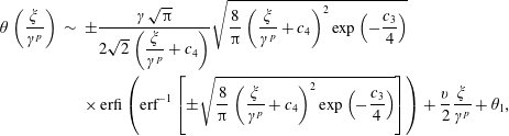



B.2 Asymptotic results for § 3.1.3
For non-zero
 $\unicode[STIX]{x1D714}$
, there are two noteworthy asymptotic regimes in (3.19).
-
(i)
$A(s)=O(\unicode[STIX]{x1D714}^{n})$
for
$n\neq -1/2$
. In this case, there exists an initial layer of width
$\unicode[STIX]{x1D714}^{n}$
, so that
$A^{\prime \prime }\sim -4/A$
and the leading-order behaviour is given by (B 5) with the scaling
$s\rightarrow s/\unicode[STIX]{x1D714}^{n}$
. -
(ii)
$A(s)=O(\unicode[STIX]{x1D714}^{n})$
for
$n=-1/2$
. The width of the region is
$\unicode[STIX]{x1D714}^{n}$
, giving the balance
$A^{\prime \prime }\sim -A-4/A$
.


B.3 Asymptotic results for § 3.2.2
Equation (3.37) can be integrated once with respect to
 $\unicode[STIX]{x1D709}$
to give
 $$\begin{eqnarray}\displaystyle {\displaystyle \frac{\text{d}\unicode[STIX]{x1D703}}{\text{d}\unicode[STIX]{x1D709}}}-{\displaystyle \frac{\unicode[STIX]{x1D6FE}}{A^{2}}}=0, & & \displaystyle\end{eqnarray}$$
where
 $\unicode[STIX]{x1D6FE}\in \mathbb{R}$
is an integration constant that has the same physical meaning as in § 3.1.2, measuring the coupling between the vortex pair separation and its change in orientation, the result of which we use to decouple (3.36),
 $$\begin{eqnarray}{\displaystyle \frac{\text{d}^{2}A}{\text{d}\unicode[STIX]{x1D709}^{2}}}+v^{2}A-{\displaystyle \frac{4}{A}}-{\displaystyle \frac{\unicode[STIX]{x1D6FE}^{2}}{A^{3}}}=0.\end{eqnarray}$$
Following the treatment of § 3.1.2, (B 8) can be integrated to obtain (B 3) with
 $$\begin{eqnarray}V(A)={\displaystyle \frac{v^{2}A^{2}}{2}}-4\ln (A)+{\displaystyle \frac{\unicode[STIX]{x1D6FE}^{2}}{2A^{2}}},\end{eqnarray}$$
and an exact implicit solution given by (3.13).
We consider the asymptotic structure of (B 8) as being dependent on
 $v$
, given that periodic solutions in
 $A$
are guaranteed for all values of
 $\unicode[STIX]{x1D6FE}$
. For
 $A(\unicode[STIX]{x1D709})=O(v^{n})$
with any non-zero
 $n$
, there are three initial layers, as follows.
-
(i) One with width
$v^{n}$
, which corresponds to the balance
$A^{\prime \prime }\sim 4/A$
, giving the leading-order behaviour (B 10)
$$\begin{eqnarray}A\left({\displaystyle \frac{\unicode[STIX]{x1D709}}{v^{n}}}\right)\sim \text{exp}\left({\displaystyle \frac{1}{8}}\left[-c_{1}-8\left(\text{erf}^{-1}\left[\pm \text{i}\sqrt{{\displaystyle \frac{8}{\unicode[STIX]{x03C0}}}\left({\displaystyle \frac{\unicode[STIX]{x1D709}}{v^{n}}}+c_{2}\right)^{2}\text{exp}\left(-{\displaystyle \frac{c_{1}}{4}}\right)}\right]\right)^{2}\right]\right),\end{eqnarray}$$
(B 11)for
$$\begin{eqnarray}\displaystyle \unicode[STIX]{x1D703}\left({\displaystyle \frac{\unicode[STIX]{x1D709}}{v^{n}}}\right) & {\sim} & \displaystyle \mp {\displaystyle \frac{\text{i}\unicode[STIX]{x1D6FE}\sqrt{\unicode[STIX]{x03C0}}}{2\sqrt{2}\left({\displaystyle \frac{\unicode[STIX]{x1D709}}{v^{n}}}+c_{2}\right)}}\sqrt{{\displaystyle \frac{8}{\unicode[STIX]{x03C0}}}\left({\displaystyle \frac{\unicode[STIX]{x1D709}}{v^{n}}}+c_{2}\right)^{2}\text{exp}\left(-{\displaystyle \frac{c_{1}}{4}}\right)}\nonumber\\ \displaystyle & & \displaystyle \times \,\text{erfi}\left(\text{erf}^{-1}\left[\pm \text{i}\sqrt{{\displaystyle \frac{8}{\unicode[STIX]{x03C0}}}\left({\displaystyle \frac{\unicode[STIX]{x1D709}}{v^{n}}}+c_{2}\right)^{2}\text{exp}\left(-{\displaystyle \frac{c_{1}}{4}}\right)}\right]\right)+\unicode[STIX]{x1D703}_{0},\end{eqnarray}$$
$c_{1},c_{2},\unicode[STIX]{x1D703}_{0}\in \mathbb{R}$
.
-
(ii) Another with width
$v^{n/2}$
, which gives the balance
$A^{\prime \prime }\sim \unicode[STIX]{x1D6FE}^{2}/A^{3}$
, leading to the dominant terms (B 12)
$$\begin{eqnarray}\displaystyle & \displaystyle A\left({\displaystyle \frac{\unicode[STIX]{x1D709}}{v^{n/2}}}\right)\sim {\displaystyle \frac{\pm 1}{\sqrt{c_{3}}}}\sqrt{\unicode[STIX]{x1D6FE}^{2}+c_{3}^{2}c_{4}^{2}+2c_{3}^{2}c_{4}{\displaystyle \frac{\unicode[STIX]{x1D709}}{v^{n/2}}}+c_{3}^{2}{\displaystyle \frac{\unicode[STIX]{x1D709}^{2}}{v^{n}}}}, & \displaystyle\end{eqnarray}$$
(B 13)for
$$\begin{eqnarray}\displaystyle & \displaystyle \unicode[STIX]{x1D703}\left({\displaystyle \frac{\unicode[STIX]{x1D709}}{v^{n/2}}}\right)\sim \tan ^{-1}\left({\displaystyle \frac{c_{3}}{\unicode[STIX]{x1D6FE}}}\left({\displaystyle \frac{\unicode[STIX]{x1D709}}{v^{n/2}}}+c_{4}\right)\right)+\unicode[STIX]{x1D703}_{1}, & \displaystyle\end{eqnarray}$$
$c_{3},c_{4},\unicode[STIX]{x1D703}_{1}\in \mathbb{R}$
.
-
(iii) The last with width
$v^{-1}$
, so that
$A^{\prime \prime }\sim -A$
, giving the leading-order behaviour (B 14)
$$\begin{eqnarray}\displaystyle & \displaystyle A(v\unicode[STIX]{x1D709})\sim c_{5}\cos (v\unicode[STIX]{x1D709})+c_{6}\sin (v\unicode[STIX]{x1D709}), & \displaystyle\end{eqnarray}$$
(B 15)for
$$\begin{eqnarray}\displaystyle & \displaystyle \unicode[STIX]{x1D703}(v\unicode[STIX]{x1D709})\sim {\displaystyle \frac{2\unicode[STIX]{x1D6FE}\sin (v\unicode[STIX]{x1D709})}{vc_{5}(c_{5}\cos (v\unicode[STIX]{x1D709})+c_{6}\sin (v\unicode[STIX]{x1D709}))}}+\unicode[STIX]{x1D703}_{2}, & \displaystyle\end{eqnarray}$$
$c_{5},c_{6},\unicode[STIX]{x1D703}_{2}\in \mathbb{R}$
.


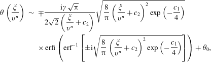








B.4 Asymptotic results for § 3.2.3
Equation (3.39) has the following asymptotic structure in
 $\unicode[STIX]{x1D714}$
for
 $A=O(\unicode[STIX]{x1D714}^{n})$
for any
 $n$
.
-
(i) An initial layer of width
$\unicode[STIX]{x1D714}^{n}$
, for
$n\neq 1/2$
, leading to the balance
$A^{\prime \prime \prime \prime }\sim (4/A)^{\prime \prime }$
. For the particular case of
$\unicode[STIX]{x1D708}(0,s)=0$
and with boundary conditions such that
$c_{1}=c_{2}=0$
, we have
$A^{\prime \prime }(s=0)-4/A(s=0)=(A^{\prime \prime }(s=0)-4/A(s=0))^{\prime }=0$
, so that the balance can be solved exactly, (B 16)for
$$\begin{eqnarray}A\left({\displaystyle \frac{s}{\unicode[STIX]{x1D714}^{n}}}\right)\sim \text{exp}\left({\displaystyle \frac{1}{8}}\left[c_{3}-8\left(\text{erf}^{-1}\left[\pm \sqrt{{\displaystyle \frac{8}{\unicode[STIX]{x03C0}}}\left({\displaystyle \frac{s}{\unicode[STIX]{x1D714}^{n}}}+c_{4}\right)^{2}\text{exp}\left(-{\displaystyle \frac{c_{3}}{4}}\right)}\right]\right)^{2}\right]\right),\end{eqnarray}$$
$c_{3},c_{4}\in \mathbb{R}$
.
-
(ii) An initial layer of width
$\unicode[STIX]{x1D714}^{-n-1}$
, for
$n\neq 1/2$
, which gives the balance
$(4/A)^{\prime \prime }\sim -A$
, leading to the dominant term (B 17)for
$$\begin{eqnarray}A(\unicode[STIX]{x1D714}^{n+1}s)\sim \text{exp}\left(-2c_{5}+\left(\text{erf}^{-1}\left[\pm {\displaystyle \frac{1}{\sqrt{2\unicode[STIX]{x03C0}}}}(\unicode[STIX]{x1D714}^{n+1}s+c_{6})^{2}\text{exp}(-2c_{5})\right]\right)^{2}\right),\end{eqnarray}$$
$c_{5},c_{6}\in \mathbb{R}$
.
-
(iii) The last initial layer has width
$\unicode[STIX]{x1D714}^{-1/2}$
, so that
$A^{\prime \prime \prime \prime }\sim A+(4/A)^{\prime \prime }$
.










Appendix C. Dispersion relation for a co-rotating hierarchy
The substitution of (4.7) into (4.6) produces a system of
 $N$
coupled equations, the form of which is most generally given by
 $$\begin{eqnarray}\unicode[STIX]{x1D714}_{n}-\unicode[STIX]{x1D6FC}\unicode[STIX]{x1D6E4}k_{n}^{2}+{\displaystyle \frac{4\unicode[STIX]{x1D6E4}}{B_{n}^{2}}}+2\unicode[STIX]{x1D6E4}\mathop{\sum }_{j\neq n}\left[{\displaystyle \frac{\exp (\text{i}\unicode[STIX]{x1D719}_{jn})}{B_{n}B_{j}}}+{\displaystyle \frac{B_{n}-B_{j}\exp (\text{i}\unicode[STIX]{x1D719}_{jn})}{B_{n}^{3}-2B_{n}^{2}B_{j}\cos (\unicode[STIX]{x1D719}_{jn})+B_{n}B_{j}^{2}}}\right]=0,\end{eqnarray}$$
where
 $\unicode[STIX]{x1D719}_{jn}=(k_{j}-k_{n})s-(\unicode[STIX]{x1D714}_{j}-\unicode[STIX]{x1D714}_{n})t+(\unicode[STIX]{x1D703}_{j}-\unicode[STIX]{x1D703}_{n})$
is the difference between the phases of
 $\unicode[STIX]{x1D707}_{j}$
and
 $\unicode[STIX]{x1D707}_{n}$
. However, given that
 $k_{n}$
and
 $\unicode[STIX]{x1D714}_{n}$
are assumed to be constant, this implies that
 $k_{n}=k$
and
 $\unicode[STIX]{x1D714}_{n}=\unicode[STIX]{x1D714}$
for every
 $\unicode[STIX]{x1D707}_{n}$
in order for
 $\unicode[STIX]{x1D719}_{jn}$
to be independent of
 $s$
and
 $t$
. In this case, the only degrees of freedom are the plane-wave amplitudes
 $B_{n}$
and phase offsets
 $\unicode[STIX]{x1D703}_{n}$
, so that
 $\unicode[STIX]{x1D719}_{jn}$
simplifies to
 $\unicode[STIX]{x1D703}_{jn}=\unicode[STIX]{x1D703}_{j}-\unicode[STIX]{x1D703}_{n}$
.
Taking the real and imaginary parts of (C 1), we find
 $$\begin{eqnarray}\displaystyle & \displaystyle \unicode[STIX]{x1D714}-\unicode[STIX]{x1D6FC}\unicode[STIX]{x1D6E4}k^{2}+{\displaystyle \frac{4\unicode[STIX]{x1D6E4}}{B_{n}^{2}}}+2\unicode[STIX]{x1D6E4}\mathop{\sum }_{j\neq n}\left[{\displaystyle \frac{B_{j}+B_{n}\cos (\unicode[STIX]{x1D703}_{jn})-2B_{j}\cos ^{2}(\unicode[STIX]{x1D703}_{jn})}{B_{j}(B_{n}^{2}-2B_{n}B_{j}\cos (\unicode[STIX]{x1D703}_{jn})+B_{j}^{2})}}\right]=0, & \displaystyle\end{eqnarray}$$
 $$\begin{eqnarray}\displaystyle & \displaystyle \mathop{\sum }_{j\neq n}\sin (\unicode[STIX]{x1D703}_{jn})\left[{\displaystyle \frac{1}{B_{n}B_{j}}}+{\displaystyle \frac{B_{j}}{B_{n}^{3}-2B_{n}^{2}B_{j}\cos (\unicode[STIX]{x1D703}_{jn})+B_{n}B_{j}^{2}}}\right]=0. & \displaystyle\end{eqnarray}$$
By the constraint that
 $\unicode[STIX]{x1D714}_{n}=\unicode[STIX]{x1D714}$
and (C 3) must hold true for all
 $n\in \{1,2,\ldots ,N\}$
, we obtain
 $2N-1$
equations for
 $2N$
unknowns. We have a single free parameter that specifies either the initial separation
 $B$
or orientation
 $\unicode[STIX]{x1D703}$
of a single satellite vortex filament. All other
 $B_{n}$
and
 $\unicode[STIX]{x1D703}_{n}$
are solved using (C 2) and (C 3).
One such solution that satisfies these constraints is
 $B_{n}=B$
and
 $\unicode[STIX]{x1D703}_{n}$
satisfying
 $$\begin{eqnarray}\unicode[STIX]{x1D703}_{n}={\displaystyle \frac{2\unicode[STIX]{x03C0}(n-1)}{N}},\quad n\in \{2,\ldots ,N+1\},\end{eqnarray}$$
which physically corresponds to the vortices being evenly distributed around the centre, so that the vortex configuration exhibits polygonal symmetry.
Substituting this result into (C 2), we obtain the dispersion relation given in (4.8).