







1. Introduction
Film boiling serves as one of the major heat transfer mechanisms, particularly in cases where high heat transfer is involved, such as quenching and spray cooling. A vapour film completely covers the heated surface during film boiling, thus preventing the liquid from coming into contact with it. The stability of this vapour film is usually determined by the amount of subcooling, liquid flow velocity and the surface condition. Many experimental and analytical studies have investigated the film boiling phenomenon over bluff bodies. The work of Bromley (Reference Bromley1950) was the first study on film boiling over a curved surface. The study of film boiling on a sphere is very critical for the safety of nuclear power plants. In the event of a nuclear power plant accident, melt fragments are generated, which subsequently penetrate the coolant. However, modelling the coolant interaction with a number of such fragment particles is challenging. The problem of film boiling on a single sphere closely resembles the situation. Therefore, a thorough study of flow film boiling on a sphere is essential.
Many research groups have carried out film boiling experiments on a sphere. Merte & Clark (Reference Merte and Clark1964) conducted experiments to study the effect of different gravity conditions on film boiling on a sphere quenched in liquid nitrogen. The heat flux was found to be proportional to  $\sqrt {g}$ for the range of gravity examined. They also concluded that the steady-state film boiling is not possible using the saturated liquid under zero gravity unless the vapour formed is removed from the vicinity of the heater surface. Rhea & Nevins (Reference Rhea and Nevins1969) experimentally investigated turbulent film boiling heat transfer over an oscillating sphere. They conducted experiments on a sphere of different diameters using liquid nitrogen at atmospheric pressure as the coolant. They concluded that, as compared with the natural convection turbulent film boiling, the oscillation of the heat transfer surface significantly enhances the heat flux for a given temperature difference. Furthermore, tests were also carried out on a sphere with different surface characteristics, and it was observed that the turbulent film boiling on a sphere is unaffected by the surface condition.
Jacobson & Shair (Reference Jacobson and Shair1970) conducted experiments on subcooled forced convection film boiling on a sphere. They found that the theoretical predictions do not agree with the experimental results if the sphere is not completely covered by the vapour film. Stevens & Witte (Reference Stevens and Witte1973) experimentally studied the transition from film boiling to nucleate boiling. The liquid was significantly subcooled in their experiments. Thus, stable film boiling was not seen and nucleate boiling started very fast. Dhir & Purohit (Reference Dhir and Purohit1978) experimentally investigated subcooled film boiling of water on a sphere. They observed that the heat transfer coefficient is not affected by the surface condition of the sphere until a stable vapour film completely covers the heated spherical surface. They also found that the minimum wall temperature required to maintain a stable vapour film increases with the amount of subcooling, but is unaffected by the flow velocity or the thermophysical characteristics of the sphere. They found that the physio-chemical nature of the spherical surface, external disturbances and diameter of the sphere play a significant role in causing partial contact in the case of subcooled film boiling.
Grigoriev, Klimenko & Shelepen (Reference Grigoriev, Klimenko and Shelepen1982) conducted film boiling experiments on a sphere using liquid nitrogen as the boiling fluid. They carried out experiments in the turbulent regime and also proposed a correlation. They claimed that their correlation agrees well with the experimental data of various research groups, which included spheres of different diameters ranging between  $0.25$ to 0.96 mm. Irving & Westwater (Reference Irving and Westwater1986) and Westwater, Hwalek & Irving (Reference Westwater, Hwalek and Irving1986) experimentally studied film boiling on a sphere and concluded that, for the large-diameter sphere of
 $D/\lambda _c>7.8$, the heat transfer coefficient is independent of the diameter of the sphere. Orozco & Witte (Reference Orozco and Witte1986) obtained the boiling curve for the flow boiling of Freon 11 past a heated copper sphere. Based on their experimental observations, they concluded that the boiling curve shows two maximum values. One maximum corresponds to the maximum heat flux during nucleate boiling, while the other one is mainly due to the transitory behaviour of the vapour wake behind the sphere. Two types of wake patterns were seen behind the sphere, which mainly depend on the heated sphere temperature. Bang & Jeun (Reference Bang and Jeun1995) conducted quenching experiments of a hot solid sphere in the subcooled dilute aqueous solution of polyethylene oxide polymer to analyse the mechanism behind the suppression of vapour explosion in the polymer solutions. Experiments on film boiling on a sphere have also been conducted using various types and concentrations of nanofluids (Lotfi & Shafii Reference Lotfi and Shafii2009; Kim et al. Reference Kim, Buongiorno, Hu and McKrell2010; Fan et al. Reference Fan, Li, Li, Zhang, Yu and Cen2015). Other experimental works primarily focus on the effect of surface morphology on film boiling (Vakarelski et al. Reference Vakarelski, Patankar, Marston, Chan and Thoroddsen2012; Vakarelski, Chan & Thoroddsen Reference Vakarelski, Chan and Thoroddsen2014; Fan et al. Reference Fan, Li, Su, Wang, Ji and Yu2016a,Reference Fan, Li, Zhang, Yu and Cenb; Jun-young et al. Reference Jun-young, Cheol, Kaviany, Sun, Moriyama and Hwan2018). Many different research groups have also attempted to study the problem of cloud cavitation behind a sphere experimentally (Arakeri Reference Arakeri1975; Brandner et al. Reference Brandner, Walker, Niekamp and Anderson2010; De Graaf, Brandner & Pearce Reference De Graaf, Brandner and Pearce2017).
The problem of film boiling on a sphere is also studied theoretically. Frederking & Clark (Reference Frederking and Clark1963) studied natural convection film boiling on a sphere. They followed the approach of Bromley (Reference Bromley1950) and proposed a correlation for the calculation of the average Nusselt number. Kobayasi (Reference Kobayasi1965) assumed the vapour layer flow to be laminar and theoretically analysed forced convection film boiling on a sphere falling downwards in a liquid pool. The Nusselt number was found to depend on the vapour Prandtl number, Reynolds Number, liquid–vapour viscosity ratio, liquid kinematic viscosity and the diameter of the sphere. They also incorporated the effect of radiation in their model. Witte (Reference Witte1968) theoretically investigated forced film boiling on a sphere. The flow was assumed to be laminar and also the velocity and temperature profiles within the vapour film were assumed to be linear. The effect of radiation was neglected. He proposed a correlation for the calculation of the average heat transfer coefficient. His proposed heat transfer coefficients for film boiling on a sphere differ from that of a cylinder only by a constant. His proposed correlation is valid only when the buoyancy effect is dominated by the forced flow. Hendricks & Baumeister (Reference Hendricks and Baumeister1969) analytically investigated natural convection film boiling on a sphere. They employed the principle of maximum entropy generation to determine the size of the vapour dome over the sphere in terms of the critical wavelength  $(\lambda _c)$.
Wilson (Reference Wilson1979) theoretically studied steady-state forced convection subcooled film boiling on a sphere. The sphere temperature was assumed to be constant. For two limiting cases, very large and small subcooling, simple analytical solutions for vapour film thickness and the Nusselt number were obtained. Epstein & Hauser (Reference Epstein and Hauser1980) analytically investigated subcooled forced convection film boiling heat transfer in the stagnation region of a sphere as well as a cylinder using the similarity as well as the perturbation theory. They proposed an expression for the vapour film thickness. After considering two extremes of very large and small subcooling values, they also proposed a correlation for the Nusselt number for subcooled forced convection film boiling. However, after comparing their correlation with the experimental data of Bromley, LeRoy & Robbers (Reference Bromley, LeRoy and Robbers1953) and Dhir & Purohit (Reference Dhir and Purohit1978), they concluded that a factor of 2.04 should be multiplied to their correlation. Gunnerson & Cronenberg (Reference Gunnerson and Cronenberg1980) analytically determined the minimum temperature and heat flux at the onset of film boiling on a sphere and a flat surface. Their predicted minimum film boiling temperature and the heat flux compared well with their experimental data. They also emphasized that these minimum conditions depend on the thermophysical properties of the heater surface and the boiling fluid. Witte & Orozco (Reference Witte and Orozco1984) theoretically investigated the effect of vapour velocity on the film boiling on a sphere and cylinder. They found that the heat transfer predictions using a quadratic velocity profile within the thin vapour film agree well with the available experimental data in comparison to a linear velocity profile. However, the heat transfer predictions using a linear as well as a quadratic velocity profile seem to be identical as the amount of subcooling increases. Bang (Reference Bang1994) applied the laminar boundary layer approximation to both the liquid and vapour phases and studied forced convection film boiling on a sphere. In the momentum equation the buoyancy term was included, which was otherwise neglected in the previous studies. Based on their study, they concluded that the vapour layer thickness reduces as the amount of subcooling increases. Their heat transfer results agreed quite well with the available experimental data. Puzina, Kryukov & Levashov (Reference Puzina, Kryukov and Levashov2024) used molecular dynamics simulations to study the evolution of the liquid–vapour interface during film boiling over a sphere.
The recent developments of various numerical techniques for the simulation of two-phase flows with accurate interface capturing have made it possible to numerically study various aspects of boiling flows. Numerical studies of Esmaeeli & Tryggvason (Reference Esmaeeli and Tryggvason2004a,Reference Esmaeeli and Tryggvasonb,Reference Esmaeeli and Tryggvasonc), Tomar et al. (Reference Tomar, Biswas, Sharma and Agrawal2005) and Son & Dhir (Reference Son and Dhir2007, Reference Son and Dhir2008) have helped in improving our understanding of boiling flows. In the past decade, many numerical studies were carried out to study the phenomenon of film boiling. However, most of these studies are focused on boiling over a flat surface (Esmaeeli & Tryggvason Reference Esmaeeli and Tryggvason2004a,Reference Esmaeeli and Tryggvasonb; Agarwal et al. Reference Agarwal, Welch, Biswas and Durst2004; Tomar et al. Reference Tomar, Biswas, Sharma and Agrawal2005; Pandey, Biswas & Dalal Reference Pandey, Biswas and Dalal2017; Premnath, Hajabdollahi & Welch Reference Premnath, Hajabdollahi and Welch2018), while very few studies focus on film boiling over curved surfaces (Singh & Premachandran Reference Singh and Premachandran2018b, Reference Singh and Premachandran2019, Reference Singh and Premachandran2021; Saito et al. Reference Saito, De Rosis, Fei, Luo, Ebihara, Kaneko and Abe2021; Thamil Kumaran & Premachandran Reference Thamil Kumaran and Premachandran2022). However, most of these studies considered two-dimensional (2-D) geometries for the simulations.
There are numerous numerical studies on single phase flow past a sphere in the literature (Johnson & Patel Reference Johnson and Patel1999; Hoffman Reference Hoffman2006; Nagata et al. Reference Nagata, Nonomura, Takahashi and Fukuda2020). However, the numerical studies of phase change over a sphere in the literature are mainly focused on unstable cavitation around a sphere (Padrino et al. Reference Padrino, Joseph, Funada, Wang and Sirignano2007; Cheng, Shao & Zhang Reference Cheng, Shao and Zhang2019). There are limited numerical works on film boiling on a sphere. Moreover, almost all of these studies have simulated 2-D axisymmetric free convection film boiling on a sphere (Yuan et al. Reference Yuan, Yang, Li and Hu2008; Arévalo et al. Reference Arévalo, Antúnez, Rebollo and Abánades2014; Phan, Ha & Park Reference Phan, Ha and Park2018).
Regarding the earlier theoretical and experimental works, it can be summarized that most of these studies focused on subcooled and saturated film boiling in the forced convection regime. Moreover, almost all of these studies were carried out for the vertical flow configuration, and studies for horizontal flow configuration are limited. In the forced convection regime the inertia force completely dominates over the buoyancy force, and the heat transfer increases due to the reduction in thickness of the vapour film. The Froude number  $(Fr={U_\infty }^2/gD)$ represents the relative relevance of the buoyancy and inertia force, where
 $U_\infty$ is the free-stream velocity,
 $g$ is the acceleration due to gravity and
 $D$ is the diameter of the sphere. For flow film boiling on a sphere at a low Reynolds number, a mixed convection regime exists. In this regime, both the inertia and buoyancy forces are comparable to each other. Therefore, in the mixed convection regime the flow and the heat transfer characteristics are governed by both the inertia and buoyancy forces. The mixed convection regime for film boiling on a sphere was theoretically analysed by Okkonen et al. (Reference Okkonen, Wennerström, Hedberg, Blomstrand, Sehgal and Frid1996), Kolev (Reference Kolev1998) and Singh, Pal & De (Reference Singh, Pal and De2022). However, there is no proper heat transfer data available as compared with the cases of natural and forced convection film boiling on a sphere. Therefore, one of the main objectives of this work is to understand the flow physics and the heat transfer during the mixed convection flow film boiling on a sphere by employing an effective and accurate numerical model for the simulation of boiling flows.
In both the vertical and horizontal film boiling on a sphere, the vapour bubbles are regularly formed and released in the wake of the sphere. Therefore, the phenomenon of film boiling on bluff bodies like a sphere is greatly influenced by the flow characteristics in the wake region for both the vertical and horizontal flow configurations. The wake characteristics behind a sphere have been extensively studied for single phase flow (Achenbach Reference Achenbach1974; Pao & Kao Reference Pao and Kao1977; Chomaz, Bonneton & Hopfinger Reference Chomaz, Bonneton and Hopfinger1993; Leweke et al. Reference Leweke, Provansal, Ormieres and Lebescond1999; Behara, Borazjani & Sotiropoulos Reference Behara, Borazjani and Sotiropoulos2011; Eshbal et al. Reference Eshbal, Rinsky, David, Greenblatt and van Hout2019). However, the wake characteristics have not been investigated for film boiling on a sphere. In the literature there are numerous analytical studies on film boiling on a sphere. However, the heat transfer in the vapour wake region, the effect of convection, the effect of surface tension and the effect of sphere diameter are often neglected in these studies. Moreover, most of these studies analyse the flow only till the separation point. The main focus of these studies is to develop a semi-empirical correlation that is compatible with the available experimental data. The results of these studies are often restricted to a very small set of flow conditions. Therefore, a very detailed numerical study will help us to further enhance our understanding of film boiling on a sphere.
The lack of any previous investigations with respect to the aforementioned aspects served as the motivation for the present study. The objective of the present work is to numerically investigate film boiling on a sphere in both the mixed and forced convection regimes. For this numerical study, the boiling flow solver employs the coupled level set and volume of fluid (CLSVOF) method of Kumar & Premachandran (Reference Kumar and Premachandran2022) for the present film boiling simulations on a three-dimensional (3-D) non-orthogonal grid. This work focuses on the influence of different flow and geometrical parameters such as the sphere diameter, degree of wall superheat and flow velocity of saturated liquid on the flow and heat transfer characteristics of film boiling on a sphere. Furthermore, the effect of surrounding liquid and vapour wakes on the flow and heat transfer characteristics of the problem has been thoroughly addressed for both the vertical and horizontal flow configurations. The present study is intended to highlight the important features of the complex phenomenon of film boiling on a sphere subjected to both horizontal and vertical flows of saturated liquid, which would otherwise be extremely difficult to ascertain solely based on an experimental or analytical study alone.
2. Problem statement
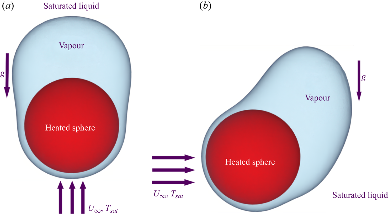
The present study numerically investigates both horizontal and vertical flow film boiling on a sphere. A schematic of the problem is shown in figure 1. The simulations have been performed for the film boiling regime of the boiling curve. In the film boiling regime a stable vapour film is always present around the heated spherical surface in both flow configurations. As shown in figure 1, for the vertical flow configuration, the gravity field acts opposite to the flow field. For the horizontal flow configuration, the gravity field acts orthogonal to the flow field. Computations were done for the saturated liquid flow Reynolds number varying between  $50$ and
 $300$.
Schematic of the forced flow film boiling on a sphere. (a) Vertical flow and (b) horizontal flow.
The paper is organized as follows. The problem formulation and the mathematical modelling are detailed in § 3. The effect of various geometrical and flow parameters on the interface evolution and the heat transfer is discussed in §§ 4.1–4.3. Subsequently, an fast Fourier transform (FFT) analysis of the space-averaged Nusselt number is also discussed in § 4.3. Finally, the results are summarized and the conclusions are provided in § 5.
3. Details of the numerical model
3.1. Computational domain
Figure 2 depicts the computational domain employed in this work for investigating both the horizontal and vertical flow film boiling on a sphere. The computational domain for the vertical flow configuration is shown in figure 2(a). For this configuration, the heated sphere of diameter  $D$ is located at
 $(10D, 10D, 10D)$ in a computational domain of size
 $(20D, 20D, 30D)$. The front
 $(y=20D)$ and the back
 $(y=0)$ boundaries of the domain are separated by a distance of
 $20D$, which leads to a confinement ratio of
 $0.05$. For the vertical flow configuration, the bottom boundary
 $(z=0)$ is the inlet and the top boundary
 $(z=30D)$ is the outlet. The distance between the inlet and outlet is
 $30D$.
Schematic of the computational domain for forced flow film boiling on a sphere. (a) Vertical flow and (b) horizontal flow.
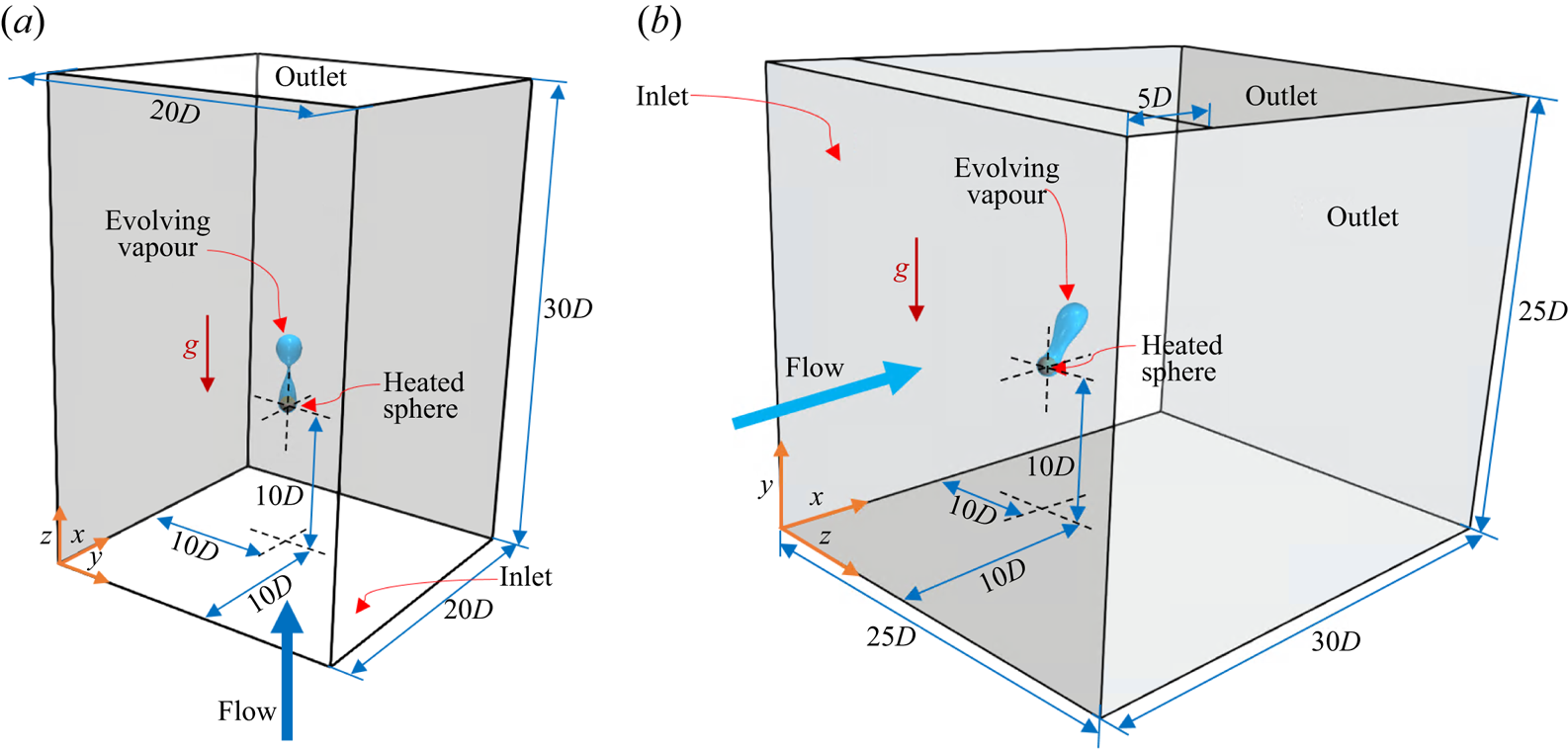
As shown in figure 2(b), for the horizontal flow film boiling case, the heated sphere is positioned at  $(10D, 10D, 10D)$ in a computational domain of size
 $(30D, 25D, 25D)$. The front
 $(z=25D)$ and the back
 $(z=0)$ boundaries of the domain are separated by a distance of
 $25D$. The left boundary
 $(x=0)$ is the inlet for the horizontal flow configuration. The top boundary of the domain
 $(y=25D)$ for the horizontal flow configuration is divided into two parts. The first part of the top boundary of
 $5D$ length is adjacent to the inlet of the domain. The second part of the top boundary of
 $25D$ length is considered an outlet. This outlet boundary at
 $y=25D$ allows the vapour bubbles rising towards the top boundary to leave the domain, especially at low Reynolds numbers for the horizontal flow configuration.
3.2. Governing equations
An unsteady, laminar and incompressible flow is analysed in the present work. Thus, the continuity, the momentum and the energy equations for the single fluid region are given as
 $$\begin{gather} \boldsymbol{\nabla}\boldsymbol{\cdot}\boldsymbol{V}=0, \end{gather}$$
 $$\begin{gather}\frac{\partial}{\partial t}(\rho\boldsymbol{V})+\boldsymbol{\nabla}\boldsymbol{\cdot}(\rho\boldsymbol{V}\boldsymbol{V})={-}\boldsymbol{\nabla} p+\boldsymbol{\nabla}\boldsymbol{\cdot}(\mu(\boldsymbol{\nabla}\boldsymbol{V}+\boldsymbol{\nabla}{\boldsymbol{V}}^T))+ \rho\boldsymbol{g}, \end{gather}$$
 $$\begin{gather}\frac{\partial}{\partial t}(\rho C_p T)+\boldsymbol{\nabla}\boldsymbol{\cdot}(\rho C_p \boldsymbol{V}T)= \boldsymbol{\nabla}\boldsymbol{\cdot}(k\boldsymbol{\nabla}T). \end{gather}$$
Here,  $\boldsymbol {V}$ is the velocity vector,
 $\rho$ is the density of the fluid,
 $p$ is the pressure,
 $\boldsymbol {g}$ is the acceleration due to gravity,
 $C_p$ is specific heat,
 $k$ is the thermal conductivity and
 $T$ is the temperature.
For the interfacial cells, the momentum equation is modified as
 \begin{equation} \frac{\partial}{\partial t}(\rho\boldsymbol{V})+\boldsymbol{\nabla}\boldsymbol{\cdot}(\rho\boldsymbol{V}\boldsymbol{V})={-}\boldsymbol{\nabla} p+\boldsymbol{\nabla}\boldsymbol{\cdot}(\mu(\boldsymbol{\nabla}\boldsymbol{V}+ \boldsymbol{\nabla}{\boldsymbol{V}}^T))+F_s+\rho\boldsymbol{g}. \end{equation}
Here,  $F_s$ denotes the surface tension force. It is included in the momentum equation as a body force term. The continuum surface force model of Brackbill, Kothe & Zemach (Reference Brackbill, Kothe and Zemach1992) is used to model the surface tension force. According to this model, the surface tension force is calculated as
 $F_s=\sigma \kappa \hat {n}\delta$, where
 $\kappa$ is the interface curvature,
 $\sigma$ is the surface tension coefficient,
 $\delta$ is the Dirac delta function and
 $\hat {n}$ represents the interface unit normal vector.
For subcooled flow boiling simulations where the liquid phase is not in a saturated condition, the energy equation is solved for both phases. However, the liquid and the interface temperatures are assumed to be constant and equal to the saturation temperature  $(T_{sat})$ for the case of saturated film boiling considered in this work (Son & Dhir Reference Son and Dhir2008). Therefore, the energy equation (3.3) is only solved for the vapour phase.
For an interfacial cell, the continuity equation is modified to account for the mass transfer across the interface as
 \begin{equation} \boldsymbol{\nabla}\boldsymbol{\cdot}\boldsymbol{V}=\left( \frac{1}{\rho_l}-\frac{1}{\rho_v} \right)\dot{m}. \end{equation}
Here,  $\dot {m}$ represents the interfacial mass flux and the subscripts
 $l$ and
 $v$ refer to the liquid and vapour phases, respectively.
The interfacial mass flux is calculated from the energy jump condition across the interface as
 \begin{equation} \dot{m}h_{lv}= {q_I}\cdot \hat{n}, \end{equation}
where  $q_I$ represents the interfacial heat flux and
 $h_{lv}$ represents the latent heat of phase change.
The expression for the interfacial mass flux,  $\dot {m}$, from (3.6) can be substituted in (3.5), to arrive at the final form of the continuity equation for an interfacial cell as
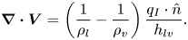 \begin{equation} \boldsymbol{\nabla}\boldsymbol{\cdot}\boldsymbol{V}=\left( \frac{1}{\rho_l}-\frac{1}{\rho_v} \right) \frac{q_I \cdot \hat{n}}{h_{lv}}. \end{equation}
3.3. Interface capturing
In this work a CLSVOF method developed by the authors (Kumar & Premachandran Reference Kumar and Premachandran2022) for unstructured polyhedral meshes is used for interface capturing.
The volume fraction  $(\alpha )$ is updated after solving the volume fraction advection equation, which is given as
 \begin{equation} \frac{\partial \alpha}{\partial t}+\boldsymbol{\nabla}\boldsymbol{\cdot} (\alpha\boldsymbol{V})={\alpha_{mt}}, \end{equation}
where  $\alpha _{mt}$ is the volume fraction generation rate in an interfacial cell. It is zero for the pure liquid cells. The rate of generation of volume fraction is calculated as
 \begin{equation} {\alpha_{mt}}=|\boldsymbol{V}_{mt}|\left(\frac{S_I}{V_c}\right), \end{equation}
where  $V_c$ is the volume of an interfacial cell,
 $S_I$ is the interface area and
 $|{\boldsymbol {V}}_{mt}|$ represents the magnitude of interface velocity due to mass transfer. An unsplit multidimensional algorithm is used for solving the volume fraction advection equation.
The advection equation for the level set field  $(\phi )$ equation is given as
 \begin{equation} \frac{\partial \phi}{\partial t}+ (\boldsymbol{V_I}\boldsymbol{\cdot}\boldsymbol{\nabla})\phi=0, \end{equation}
where  $\boldsymbol {V_I}={\boldsymbol {V}}_{mt}+\boldsymbol {V}$, is the sum of the interface velocity due to mass transfer and the cell fluid velocity.
The updated level set and volume fraction fields are utilized to geometrically reconstruct the interface in all the interfacial cells. The level set field is utilized to evaluate the unit interface normal for all the interfacial cells. The unit interface normal is calculated as
 \begin{equation} \hat{n}=\frac{\boldsymbol{\nabla}\phi}{|\boldsymbol{\nabla}\phi|}. \end{equation}
The level set field does not remain a signed distance function after every time step. Therefore, the level set field needs to be reinitialized geometrically after every time step.
Any fluid property  $(\lambda )$ is evaluated using the Heaviside function
 $H(\phi )$ as given in (3.12) to avoid any numerical instability caused by an abrupt property change across the interface:
 \begin{equation} \lambda=\lambda_l+(\lambda_l-\lambda_v)H(\phi). \end{equation}
Here, the subscripts  $l$ and
 $v$ refer to liquid and vapour phases, respectively. The Heaviside function used in this study is given as (Son & Hur Reference Son and Hur2002)
 \begin{equation} \left. \begin{array}{@{}ll@{}} \displaystyle H(\phi)=1 & \mbox{if}\ \phi\geqslant\epsilon,\\ \displaystyle H(\phi)=0.5+\dfrac{\phi}{2\epsilon}+\dfrac{1}{2{\rm \pi}}\sin\left(\dfrac{{\rm \pi}\phi}{\epsilon}\right) & \mbox{if}\ |\phi|\leqslant\epsilon,\\ \displaystyle H(\phi)=0 & \mbox{if }\phi\leqslant\epsilon. \end{array}\right\} \end{equation}
Here,  $\epsilon$ is the interface thickness, which is commonly considered to be
 $1.5h$, where
 $h$ is taken to be the cube root of the interfacial cell volume. Additionally, the
 $\hat {n}\delta$ term in the volumetric surface tension force calculation is replaced with
 $\boldsymbol {\nabla } H$. Thus, the volumetric surface tension force can be rewritten as
 $F_s=\sigma \kappa \hat {n}\delta =\sigma \kappa \nabla H$. Here, the interface curvature is calculated as
 \begin{equation} \kappa={-}\boldsymbol{\nabla}\boldsymbol{\cdot}\hat{n}. \end{equation}
The heat flux along the interface normal is given as
 \begin{equation} q_I=k_v\left(\frac{T_v-T_I}{\Delta\zeta}\right)-k_l\left(\frac{T_I-T_l} {\Delta\zeta}\right). \end{equation}
Here, the subscripts  $l$,
 $v$ and
 $I$ refer to the liquid, vapour and interface, respectively;
 $\Delta \zeta$ represents the distance from the interface to the cell centroid. In the present case of saturated film boiling,
 $T_I=T_l=T_{sat}$ (Welch & Wilson Reference Welch and Wilson2000; Agarwal et al. Reference Agarwal, Welch, Biswas and Durst2004; Tomar et al. Reference Tomar, Biswas, Sharma and Agrawal2005; Son & Dhir Reference Son and Dhir2008; Singh & Premachandran Reference Singh and Premachandran2018a; Thamil Kumaran & Premachandran Reference Thamil Kumaran and Premachandran2022). Therefore, the interfacial heat flux can be rewritten as
 \begin{equation} q_I=k_v\left(\frac{T_v-T_I}{\Delta\zeta}\right). \end{equation}
The expression for  $q_I$ obtained in (3.16) can be substituted in (3.6) to calculate the interfacial mass flux as
 \begin{equation} \dot{m}=\frac{k_v}{h_{lv}}\left(\frac{T_v-T_I}{\Delta\zeta}\right). \end{equation}
3.4. Solver details
An in-house boiling flow solver, developed by the authors in their previous work (Kumar & Premachandran Reference Kumar and Premachandran2022), is used for the present simulations. The flow solver is based on the finite volume method. It employs the CLSVOF method for interface capturing. For the pressure–velocity coupling, the SIMPLE algorithm of Patankar (Reference Patankar1980) was used. The QUICK scheme is used to discretize the convective terms in the momentum and energy equations. For time marching, a second-order accurate backward explicit scheme is used. The Courant–Friedrichs–Lewy condition, along with the surface tension, gravity and viscous forces, restricts the time step size used for the present simulations. It is calculated as
 \begin{equation} \Delta t<\min\left\{\frac{h}{||\boldsymbol{V}||},\frac{\rho h^2}{\mu},{\left(\frac{h}{||\boldsymbol{g}||}\right)}^{0.5},\left(\frac{(\rho_l+\rho_g)h^3}{4{\rm \pi}\sigma}\right)^{0.5}\right\}. \end{equation}
The time step size in boiling flow simulations is highly influenced by the cell size  $(h)$ as indicated in (3.18). Furthermore, a very fine grid size is required to accurately capture the interface.
3.5. Boundary and initial conditions
The convective outlet boundary condition of Orlanski (Reference Orlanski1976) is used at the outlet for both the vertical and horizontal flow configurations. The convective outlet boundary condition is given as
 \begin{equation} \frac{\partial \gamma}{\partial t}+U_C\frac{\partial \gamma}{\partial n}=0. \end{equation}
Here,  $U_C$ is the convective velocity,
 $\gamma$ denotes any variable of interest other than the pressure and
 $\partial \gamma /\partial n$ represents the gradient of any variable perpendicular to the outlet of the domain. As recommended by Yoshida, Watanabe & Nakamura (Reference Yoshida, Watanabe and Nakamura1993) and Sohankar, Norberg & Davidson (Reference Sohankar, Norberg and Davidson1998), the value of
 $U_C$ was set equal to
 $U_\infty$ in the present study. This assumption of
 $U_C=U_\infty$ was also used by Breuer (Reference Breuer1998a,Reference Breuerb) and Giannenas, Laizet & Rigas (Reference Giannenas, Laizet and Rigas2022) in their numerical studies. The pressure is constant at the outlet boundaries. The no-slip boundary condition is specified on the heated sphere. A uniform velocity boundary condition is applied at the inlet, whereas a free slip boundary condition is applied at all the other boundaries of the domain
 $(v_{perp}=0.0, \partial v_{parl}/\partial n=0.0)$, where
 $(perp)$ and
 $(parl)$ refer to the velocity components perpendicular and parallel to the boundary. A uniform film of vapour of
 $0.1D$ thickness completely encloses the heated spherical surface initially. The temperature within the vapour film is initialized to vary linearly between the heated sphere temperature and the temperature of the surrounding saturated liquid. The heated spherical surface is considered to be at a constant temperature of
 $T_{wall}=T_{sat}+\Delta T_{sup}$, where
 $T_{sat}$ represents the saturation temperature and
 $\Delta T_{sup}$ specifies the degree of wall superheat. Initially, in the computational domain, the velocity is set to zero while the pressure varies hydrostatically. In the present study the numerical simulations were run for multiple vapour bubble ebullition cycles. This ensures that the heat transfer characteristics of the problem are not affected by the assumed initial conditions.
3.6. Nusselt number calculation
In the present study the temporally and spatially averaged Nusselt numbers are employed to estimate the heat transfer. They are evaluated as, for the local Nusselt number,
 \begin{equation} Nu_D=\left.-\frac{D}{\Delta T_{sup}}\frac{\partial T}{\partial n}\right|_w, \end{equation}
where  $\partial T/\partial n |_w$ represents the gradient of temperature normal to the sphere; for the space-averaged Nusselt number,
 \begin{equation} Nu_{spaceAvg}= \frac{1}{4{\rm \pi}}{\int_0}^{2{\rm \pi}} {\int_0}^{\rm \pi}Nu_D\sin{\alpha} \, {\rm d}\alpha \,{\rm d}\beta; \end{equation}
and for the space–time-averaged Nusselt number,
 \begin{equation} Nu_{timeAvg}=\frac{1}{t}{\int_0}^t Nu_{spaceAvg}\,{\rm d}t. \end{equation}
3.7. Fluid properties and simulation parameters
For all the simulations in this work, water at  $p_{sat}={21.9}\ \textrm {MPa}$,
 $T_{sat}={646}\ \textrm {K}$ is used as the boiling fluid. These same fluid properties were also used by Tomar et al. (Reference Tomar, Biswas, Sharma and Agrawal2005) for their film boiling simulations.
The simulations were done for the Reynolds numbers varying in the range of 50–300 for different sphere diameters at various wall superheats. For the corresponding Reynolds number values, the flow regimes vary from mixed convection to forced convection. Both the buoyancy and inertia forces are comparable in the mixed convection regime, and only the inertia force dominates in the forced convection regime. The relative dominance of both these forces is characterized by the Froude number  $(Fr)$. In general, many flow and geometrical parameters can affect the phenomenon of film boiling on a sphere. Therefore, different parameters were varied in this work in order to get a complete understanding of the flow physics of film boiling on a sphere. The effect of saturated liquid flow velocity at the inlet is quantified in terms of Reynolds number
 $(Re_D=\rho _l U_\infty D/\mu _l)$. The effects of dimensionless sphere diameter and the dimensionless wall superheat are quantified in terms of
 $\tilde {D}=D/\lambda _0$ and
 ${Ja^*}=Ja_v/Pr_v$, respectively. Here,
 $Ja_v=C_{pv}\Delta T_{sup}/h_{lv}$ is the Jakob number,
 $Pr_v=\mu _v{C_{pv}}/k_v$ is the Prandtl number,
 $h_{lv}$ is the latent heat of vaporization,
 $D$ is the diameter of the heated sphere,
 $U_\infty$ is the velocity of the incoming saturated liquid,
 $\mu _l$ and
 $\rho _l$ are the liquid viscosity and density, respectively,
 $C_{pv}$,
 $\mu _v$ and
 $k_v$ are the specific heat, vapour viscosity and thermal conductivity, respectively, whereas
 $g$ is the acceleration due to gravity and
 $\lambda _0=\sqrt {\sigma /(\rho _l-\rho _v)g}$ is the capillary length scale of the problem.
In the present work, simulations were performed for four different Reynolds number values of  $Re_D=50, 100, 200$ and
 $300$. The dimensionless sphere diameter values considered are
 $\tilde {D}=0.5, 1.0$ and
 $5$, whereas the dimensionless wall superheat values considered in this numerical study are
 ${Ja^*}=0.3,0.6$ and
 $0.9$.
The effect of thermal radiation-induced heat transfer is critical for stable film boiling on hot surfaces. Some analytical investigations have also incorporated the effect of radiation. However, as pointed out by Singh & Premachandran (Reference Singh and Premachandran2018b, Reference Singh and Premachandran2021) and Kumar & Premachandran (Reference Kumar and Premachandran2023), the effect of radiative heat transfer is almost absent at high pressures if the heater surface is assumed to be well polished.
3.8. Grid independence study
A typical computational grid used for the present numerical work is presented in figure 3 for the vertical flow configuration. Many numerical studies on flow past a sphere as well as cavitating flow past a sphere have employed a similar type of grid (Ploumhans et al. Reference Ploumhans, Winckelmans, Salmon, Leonard and Warren2002; Pal et al. Reference Pal, Sarkar, Posa and Balaras2017; Cheng et al. Reference Cheng, Shao and Zhang2019). Figure 3 shows the grid for the entire computational domain on two perpendicular planes. Additionally, a zoomed view of the grid in the vicinity of the sphere is also shown in figure 3. Hexahedral cells are used throughout the computational domain.
A typical computational grid used for film boiling simulations.
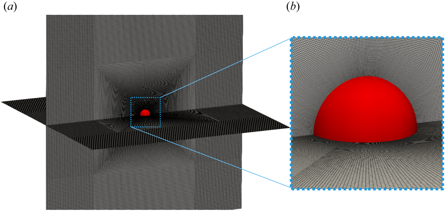
For the grid independence study, vertical flow film boiling simulations were performed for  ${Ja^*}=0.6$,
 $Re_D=50$ and
 $\tilde {D}=1.0$ till
 $t= 0.5\ \textrm {s}$. As shown in table 1, three different grids were employed to conduct this test, which is defined by the size of the cell adjacent to the heated spherical surface. The smallest cell sizes considered for the grid independence test for the vertical flow film boiling in the radial direction are
 $0.002D$,
 $0.001D$ and
 $0.0005D$, where
 $D$ is the diameter of the sphere. Here
 $N_{cell}$ and
 $N_{quadSphere}$ in table 1 denote the total number of cells in the entire computational domain and the total number of quadrilateral surface cells on the heated spherical surface, respectively. It is evident that the difference in the
 $Nu_{timeAvg}$ values obtained using mesh 2 and mesh 3 is negligible. Thus, mesh 2 will serve as an optimal choice for the boiling flow simulations over a sphere without compromising much with accuracy while incurring low computing costs. A similar grid independence study was also carried out for the horizontal flow configuration. The details of the grid independence study for the horizontal flow configuration are not given here for the sake of brevity.
Details of the grid independence study.

3.9. Validation of the numerical model
The present CLSVOF method and the boiling flow solver were validated against the experimental results of Sakurai, Shiotsu & Hata (Reference Sakurai, Shiotsu and Hata1990). The simulations were carried out for pool film boiling on a cylinder of diameter  ${1.2}\ \textrm {mm}$, using liquid nitrogen at
 ${1.836}\ \textrm {MPa}$ as the boiling fluid. These simulations were performed for four different wall superheat
 $(\Delta T_{sup})$ values till
 $t=1.0\ \textrm {s}$. Subsequently, the
 $Nu_{timeAvg}$ was evaluated and compared with the experimental results of Sakurai et al. (Reference Sakurai, Shiotsu and Hata1990) as shown in table 2.
Validation of the present numerical results against the experimental results of Sakurai et al. (Reference Sakurai, Shiotsu and Hata1990).
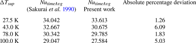
Additionally, the present numerical model was also validated against the experimental data of Liu & Fukuda (Reference Liu and Fukuda2008). The validation study was carried out for vertical flow film boiling over a cylinder in the mixed convection regime, using water at 294 kPa as the boiling fluid. The simulations were performed for three different  $\sqrt {Fr}$ at different
 $\Delta T_{sup}$ and
 $\tilde {D}=2.1$ until
 $t=1.0\ \textrm {s}$. The
 $Nu_{timeAvg}$ was calculated for different
 $\sqrt {Fr}$ and compared with the experimental results of Liu & Fukuda (Reference Liu and Fukuda2008) in table 3.
Validation of the present numerical results against the experimental results of Liu & Fukuda (Reference Liu and Fukuda2008).
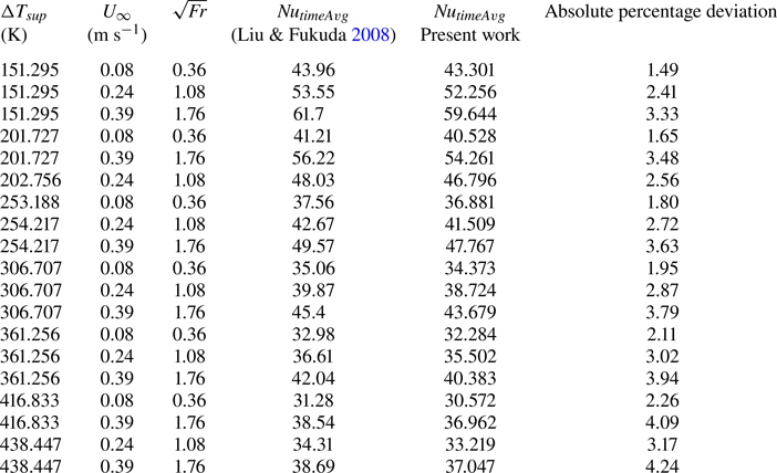
As shown in table 2, the maximum absolute percentage deviation between the present numerical results and the experimental data of Sakurai et al. (Reference Sakurai, Shiotsu and Hata1990) is  $6.09\,\%$. Similarly, as shown in table 3, the maximum absolute percentage deviation between the present numerical result and the experimental data of Liu & Fukuda (Reference Liu and Fukuda2008) is
 $4.24\,\%$. This small absolute percentage deviation between the numerical and experimental results can be due to the use of constant fluid properties in the present simulations. Overall, the present numerical results are in good agreement with the experimental results of both Sakurai et al. (Reference Sakurai, Shiotsu and Hata1990) and Liu & Fukuda (Reference Liu and Fukuda2008).
Furthermore, the numerical model used in the present work was thoroughly validated in the earlier work of the current authors (Kumar & Premachandran Reference Kumar and Premachandran2022). The CLSVOF interface capturing method was validated for different advection test cases. For the phase change problems, the boiling flow solver with the CLSVOF interface capturing method was used for 2-D and 3-D pool film boiling on a flat plate and a cylinder at various wall superheats. The heat transfer predictions of these cases were in excellent agreement with the available semi-empirical correlations in the literature. Thus, the present boiling flow solver was validated with the experimental and numerical results available in the literature before performing the present film boiling simulations on a sphere. For further details of the validation of the boiling flow solver, the reader can refer to the work of Kumar & Premachandran (Reference Kumar and Premachandran2022).
4. Results and discussion
This section discusses the effect of various geometrical and flow variables on the flow features and the heat transfer characteristics for flow film boiling on a sphere. The saturated liquid flow Reynolds number  $(Re_D)$ is varied in the range of 50–300. The range of dimensionless wall superheat
 $({Ja^*})$ considered is
 $0.3$ to
 $0.9$. The dimensionless sphere diameter
 $(\tilde {D})$ is varied from
 $0.5$ to
 $5$.
4.1. Effect of Reynolds number
Four different values of  $Re_D$ viz. 50, 100, 200 and 300 are considered in this work to study the effect of saturated liquid flow velocity on the flow and heat transfer characteristics of the problem. The corresponding
 $\sqrt {Fr}$ are
 $0.6, 1.2, 2.4$ and
 $3.6$, respectively. The Froude number governs the relative dominance of the inertia and buoyancy forces. However, it should be highlighted here that the exact value of
 $\sqrt {Fr}$, which differentiates between the mixed and the forced convection regime for film boiling on a sphere, is not known from the previous analytical studies. For instance, Kobayasi (Reference Kobayasi1965) and Epstein & Hauser (Reference Epstein and Hauser1980) analytically analysed forced convection film boiling on a sphere and gave a correlation for Nusselt number calculation. However, they did not mention any specific range of
 $\sqrt {Fr}$ that falls in the mixed convection regime. In the present section, the results obtained for different
 $Re_D$ with
 $\tilde {D}=1$ and
 ${Ja^*}=0.6$ are discussed.
Figure 4 illustrates the evolution of the interface for the vertical flow film boiling on a sphere of dimensionless diameter  $\tilde {D}=1$ at different
 $Re_D$ and
 ${Ja^*}=0.6$. For
 $Re_D=50$, the interface evolution closely resembles the interface evolution in the natural convection regime of film boiling (Kumar & Premachandran Reference Kumar and Premachandran2023). This is obvious because, at low Reynolds number, the vapour bubbles are periodically formed and detached from the vapour film due to the Rayleigh–Taylor instability. The vapour is continuously generated in the vapour film around the sphere, which tends to accumulate in the upper region of the sphere due to the buoyancy force. Due to the inertia force, the vapour mass is continually elongated in the direction of the flow while it is still connected to the film due to the surface tension force. The bubble is eventually released after it attains a specific size. When the bubble departs, the leftover vapour mass tends to slowly recoil back towards the sphere, and a new bubble starts developing. The interface evolution in this case closely resembles that in the natural convection regime (Kumar & Premachandran Reference Kumar and Premachandran2023). However, compared with the natural convection regime, the interface in the present situation is more extended along the flow direction. Additionally, the vapour mass does not recoil back completely to the heated sphere after the vapour bubble is pinched off even for
 $Re_D=50$ (for more detail, please watch supplementary movie 1 available at https://doi.org/10.1017/jfm.2024.514 provided with this paper). For
 $Re_D=100$, the interface evolution is very similar to that at
 $Re_D=50$. However, the effect of inertia is more pronounced in this case as the vapour column is stretched more along the flow direction in the wake region of the sphere as compared with
 $Re_D=50$. The dominance of the inertial force can also be ascertained by the fact that the recoil of the remaining vapour mass after bubble pinch-off is limited to a region far downstream of the sphere. It can also be seen that the vapour film thickness is reduced in this case as the Reynolds number is increased for the same dimensionless wall superheat. Also, the frequency of the periodic vapour bubble formation and release increases at
 $Re_D=100$ as compared with that at
 $Re_D=50$.
Interface evolution for the vertical flow configuration for  $\tilde {D}=1$ and
 ${Ja^*}=0.6$ for various
 $Re_D$. Results are shown for (a)
 $Re_D=50$,
 $\sqrt {Fr}=0.6$; (b)
 $Re_D=100$,
 $\sqrt {Fr}=1.2$; (c)
 $Re_D=200$,
 $\sqrt {Fr}=2.4$; (d)
 $Re_D=300$,
 $\sqrt {Fr}=3.6$.
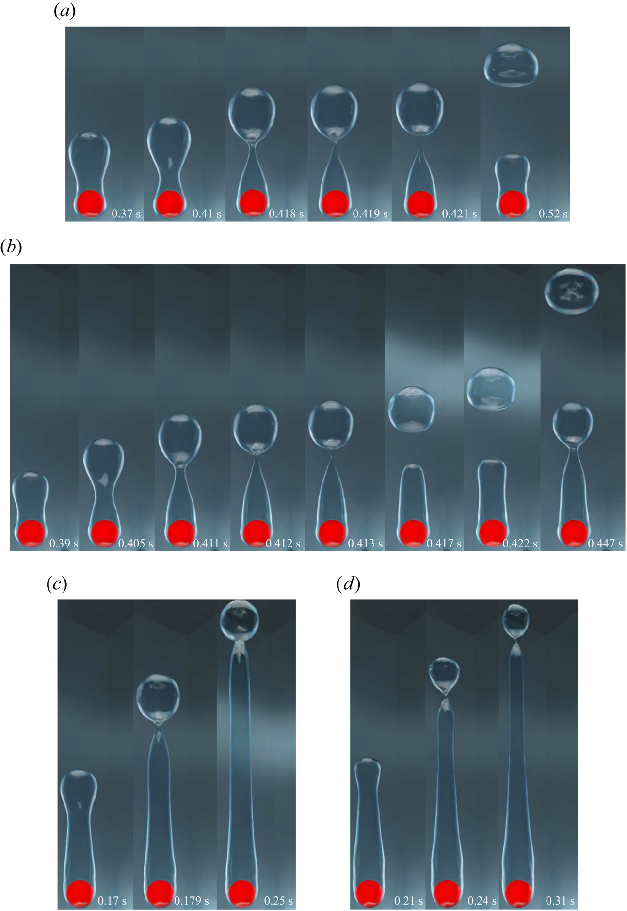
For the vertical flow film boiling, as the saturated liquid flow velocity is further increased, i.e. for  $Re_D=200$ and
 $300$, the vapour mass is observed to elongate along the flow direction to form a vapour column as shown in figures 4(c) and 4(d), under the action of strong inertial force. However, small vapour bubbles are randomly pinched off from the vapour column's tail. The recoil of the vapour mass towards the sphere is completely absent in these two cases, which shows that the buoyancy force is dominated by the inertial force. Thus, for the vertical flow film boiling on a sphere, the behaviour of the vapour wake downstream of the sphere changes significantly at
 $Re_D=200$ and
 $300$ as compared with that at
 $Re_D=50$ and
 $100$. This demonstrates an interplay between the inertia and the buoyancy force as the
 $Re_D$ is increased while the
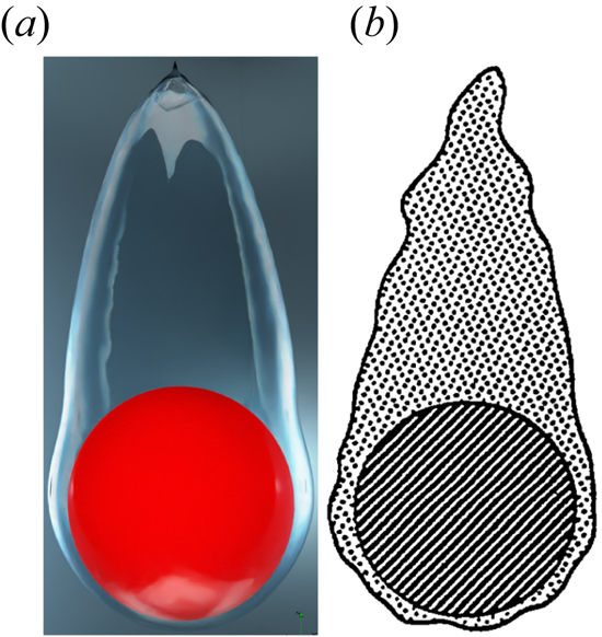
 ${Ja^*}$ is kept constant. A qualitative comparison of the present interface evolution with that of Liu & Theofanous (Reference Liu and Theofanous1996) for completely saturated film boiling on a sphere is presented in figure 5 for
 $Re_D=100$,
 $\tilde {D}=1$ and
 ${Ja^*}=0.6$. It is clear from this figure that the numerically obtained interface agrees appreciably well with their schematic.
Comparison of the present numerical result at  $Re_D=100, \sqrt {Fr}=1.2$ for
 $\tilde {D}=1$ and
 ${Ja^*}=0.6$, with the conceptual illustration of Liu & Theofanous (Reference Liu and Theofanous1996) presented based on their experimental observation for a completely saturated vertical flow film boiling on a sphere.
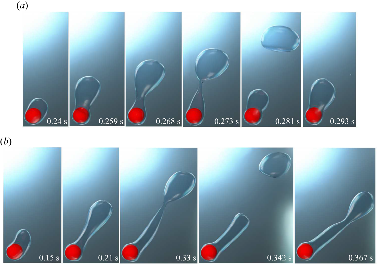
Figures 6 and 7 illustrate the effect of Reynolds number on the evolution of the interface for the horizontal flow film boiling on a sphere. For  $Re_D=50$, the interface seems to evolve under the combined action of both the inertial and buoyancy forces. The vapour bubbles are continuously formed and released in a cycle from the vapour film due to the Rayleigh–Taylor instability. This periodic vapour ebullition cycle consists of vapour proliferation on the top of the heated spherical surface followed by a vapour mass pinch-off and recoil towards the heated spherical surface. However, compared with the upward flow case, the vapour bubble pinch-off location for the horizontal flow case is shifted slightly to the top-right region of the sphere. Additionally, as shown in figure 6(a) at
 $t=0.259\mbox{--}0.293\ \textrm {s}$, a vapour bulge is evident near the bottom-right region of the sphere. This indicates a non-uniform vapour generation around the heated sphere for the horizontal flow configuration at
 $Re_D=50$ (for more detail, please watch supplementary movie 2 provided with this paper). As shown in figure 6(b), the effect of inertial force is more pronounced at
 $Re_D=100$ as the developing interface is elongated along the diagonal direction. In this figure at time
 $t=0.33\ \textrm {s}\mbox{--}0.367 \textrm {s}$, it can be seen that as soon as the bubble departs at
 $t=0.33 \textrm {s}$, the interface does not recoil back completely towards the heated sphere as seen for
 $Re_D=50$. Instead, a new vapour bubble starts forming at the tail of the elongated column, which again pinches off. Another interesting observation is that for the horizontal flow configuration, the vapour film thickness is not uniform over the sphere. A thick vapour film is observed near the bottom of the sphere as compared with the top region of the sphere.
Interface evolution for the horizontal flow configuration for  $\tilde {D}=1$ and
 ${Ja^*}=0.6$ at various
 $Re_D$. Results are shown for (a)
 $Re_D=50$,
 $\sqrt {Fr}=0.6$; (b)
 $Re_D=100$,
 $\sqrt {Fr}=1.2$.
Interface evolution for the horizontal flow configuration for  $\tilde {D}=1$ and
 ${Ja^*}=0.6$ at various
 $Re_D$. Results are shown for (a)
 $Re_D=200$,
 $\sqrt {Fr}=2.4$; (b)
 $Re_D=300$,
 $\sqrt {Fr}=3.6$.
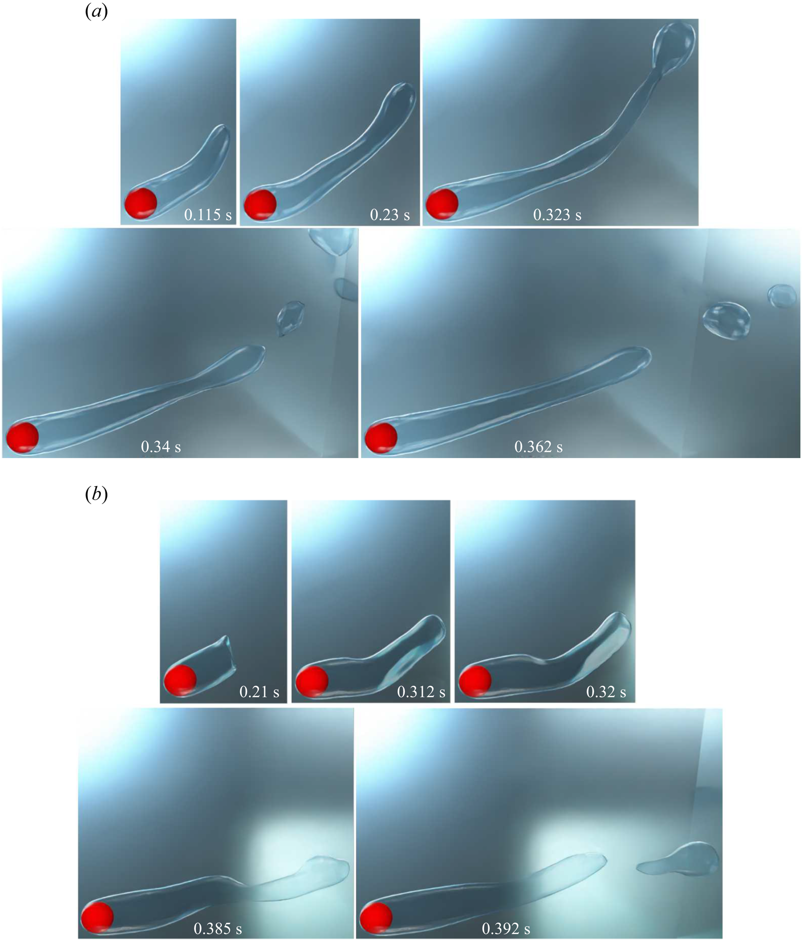
The interface evolution for  ${Ja^*}=0.6$ and
 $\tilde {D}=1$ for
 $Re_D=200$ and
 $300$ is shown in figure 7 for the horizontal flow configuration. As shown in this figure, the thin vapour film region is limited to the region surrounding the front stagnation point, whereas the vapour wake completely moves to the back of the sphere at high flow velocities of saturated liquid. This shows a considerable dominance of the inertial force over the buoyancy force at
 $Re_D=200$ and
 $300$. The vapour bubble formation and release at
 $Re_D=200$ and
 $300$ is predominantly governed by the Kelvin–Helmholtz instability as compared with the Rayleigh–Taylor instability at a low Reynolds number. For
 $Re_D=200$, a long vapour wake is seen to develop under the influence of inertial force. However, it also tends to rise against gravity at time
 $t=0.323\ \textrm {s}$ due to the buoyancy force. Eventually, a stable vapour wake develops downstream of the sphere, and the vapour bubbles of random size are constantly torn away from the tail of this vapour wake. The vapour wake at
 $Re_D=300$ is particularly unstable as compared with
 $Re_D=200$. This unstable vapour wake is seen to flutter along with the flow, and due to this motion, random vapour bubbles of different sizes are torn away from this vapour wake as shown in figure 7(b) for
 $Re_D=300$ at time
 $t=0.392\ \textrm {s}$. This suggests a dominance of the inertial force over the buoyancy force at
 $Re_D=300$. In general, it can be seen that in the horizontal flow configuration, the interface evolution is largely affected by the inlet velocity of the saturated liquid, as compared with the vertical flow configuration. The vapour bubble dynamics is significantly influenced by inertial force even at
 $Re_D=50$.
The departure diameter of the vapour bubble  $(D_{vb})$ was calculated for the cases where the vapour bubble evolves periodically for both the vertical and horizontal flow configurations. For the vertical flow configuration, at
 $Re_D=50$ and
 $100$,
 $D_{vb}$ is
 $1.902D$ and
 $1.803D$, respectively. For the horizontal flow configuration, at
 $Re_D=50$ and
 $100$,
 $D_{vb}$ is
 $2.041D$ and
 $1.879D$, respectively. These results show that
 $D_{vb}$ decreases as the vapour bubble pinch-off location shifts downstream of the sphere at
 $Re_D=100$ as compared with
 $Re_D=50$. Additionally,
 $D_{vb}$ is higher for the horizontal flow configuration as compared with the vertical flow configuration for the same
 $Re_D$.
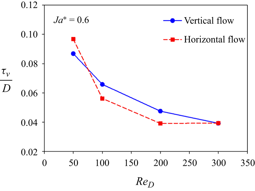
The variation of the dimensionless time-averaged vapour film thickness at the front stagnation point of the sphere  $(\tau _v/D)$ with
 $Re_D$ at
 ${Ja^*}=0.6$ and
 $\tilde {D}=1$ is shown in figure 8 for both the vertical and horizontal flow configurations. The
 $\tau _v/D$ decreases as the
 $Re_D$ increases for both the vertical and horizontal flow configurations. Here
 $\tau _v/D$ is higher for the horizontal flow configuration as compared with the vertical flow configuration at
 $Re_D=50$. For the horizontal flow configuration,
 $\tau _v/D$ is less at
 $Re_D=200$ and
 $300$ as compared with the vertical flow configuration. However,
 $\tau _v/D$ at
 $Re_D=300$ is almost the same for both flow configurations.
Variation of the dimensionless time-averaged vapour film thickness  $(\tau _v/D)$ at the front stagnation point of the sphere versus
 $Re_D$ at
 ${Ja^*}=0.6$ and
 $\tilde {D}=1$.
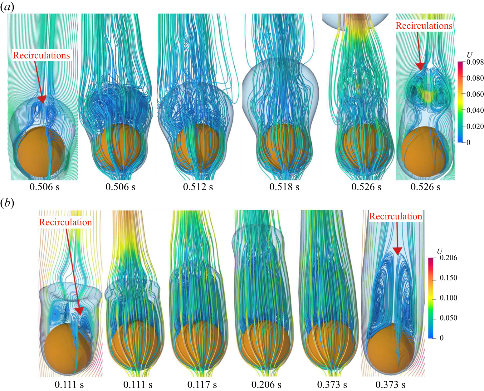
Most of the earlier analytical studies argued that a detailed analysis of the vapour wake region is not necessary as the heat transfer in the vapour wake region is negligible as compared with the heat transfer from the heated surface in the thin film region. Thus, most of the analytical studies underestimated the experimental data available in the literature. Therefore, in the present work a detailed investigation of the flow in the vapour wake region is carried out for both the horizontal and vertical flow configurations. The instantaneous 3-D streamlines in the vapour wake are shown in figure 9 for the vertical flow configurations at different  $Re_D$ and
 ${Ja^*}=0.6$ for
 $\tilde {D}=1$. At
 $Re_D=50$, a recirculation region is observed inside the vapour wake at
 $0.506\ \textrm {s}$, which gradually fades away as seen at
 $0.518\ \textrm {s}$. As the vapour bubble departs and the interface tends to recoil back towards the heated sphere, again, some recirculations can be seen at
 $0.526\ \textrm {s}$. This regular formation of a recirculation region can be ascribed to the periodic vapour bubble ebullition cycle at
 $Re_D=50$ owing to the dominance of buoyancy force over inertial force (for more detail, please watch supplementary movie 3 provided with this paper). As illustrated in figure 9(b), at
 $Re_D=300$, the 3-D streamline plot around the heated sphere shows the presence of a recirculation region in the vapour wake at all times. Gradually, this recirculation region gets elongated along the flow direction until it has reached a specified size at around
 $0.373\ \textrm {s}$. However, the vapour film continues to elongate along the flow direction even after the recirculation region has attained a constant size.
Three-dimensional streamlines within the vapour wake for the vertical flow configuration at different  $Re_D$ for
 $\tilde {D}=1$ and
 ${Ja^*}=0.6$. Results are shown for (a)
 $Re_D=50$
 $(\sqrt {Fr}=0.6)$ and (b)
 $Re_D=300$
 $(\sqrt {Fr}=3.6)$.
For the vertical flow configurations, recirculations are formed periodically in the vapour wake region at  $Re_D=50$. However, the recirculation region attains a constant size at
 $Re_D=300$. Therefore, in the present work the separation angle is measured for the cases where a constant-size recirculation region is observed. The separation angle,
 $\theta _s$, is measured from the front stagnation point of the sphere. For
 $Re_D=200$ and
 $300$,
 $\theta _s$ is
 $123.27^{\circ }$ and
 $114.84^{\circ }$, respectively. Under the increased effect of the inertia force at
 $Re_D=300$, the separation angle within the vapour phase decreases as compared with
 $Re_D=200$.
The instantaneous 3-D streamlines around the sphere in the vapour wake are shown in figure 10 for the horizontal flow configuration at different  $Re_D$ at
 ${Ja^*}=0.6$ and
 $\tilde {D}=1$. It was discussed earlier that the vapour bubble evolution cycle is quasi-steady at a lower Reynolds number for the horizontal flow configuration. Therefore, many streamlines can be seen in the top-right region of the sphere when a new bubble starts developing at time
 $t=0.419, 0.425\ \textrm {{s}}$. At time
 $t=0.452\ \textrm {s}$ in figure 10(a), these streamlines are observed to separate out from each other as the vapour bubble starts growing. Eventually, under the combined effect of the surface tension force and the buoyancy force, a neck starts developing, which restricts the vapour flow into the growing bubble. Hence, as shown in figure 10(a), a high-velocity field is observed in the neck region at time
 $t=0.499\ \textrm {s}$. As the vapour bubble departs, the interface tends to recoil back towards the heated sphere. This interfacial motion leads to the formation of new recirculations in the vapour wake at time
 $t=0.505\ \textrm {s}$ as shown in figure 10(a), which in due course grows with time as a new vapour bubble begins to form at the same place (for more detail, please watch supplementary movie 4 provided with this paper). For
 $Re_D=300$, recirculations can be seen within the vapour phase in the wake region of the sphere at all times. This observation indicates a strong coupling between the liquid and vapour wake, which is governed by a strong interplay between the inertial and buoyancy force at a higher Reynolds number. Interestingly, for the horizontal flow configuration at
 $Re_D=50$, the 3-D streamlines are concentrated near the bottom region of the sphere as shown in figure 10(a), where an interfacial bulge was present as discussed earlier. This indicates that the vapour generation is not uniform over the heated sphere at a low Reynolds number of
 $50$ for the horizontal flow configuration. However, no vapour bulge was observed at the higher Reynolds numbers of
 $200$ and
 $300$ where a uniform vapour film completely engulfs the region near the front stagnation point of the heated sphere. As shown in figure 10(b), for
 $Re_D=300$, recirculations are present near the rear stagnation point of the sphere. Contrary to the vertical flow case at
 $Re_D=300$, for the horizontal flow case, the shape of the recirculations present in the vapour wake continuously changes with time.
Three-dimensional streamlines within the vapour wake for the horizontal flow configuration at different  $Re_D$ for
 $\tilde {D}=1$ and
 ${Ja^*}=0.6$. Results are shown for (a)
 $Re_D=50$
 $(\sqrt {Fr}=0.6)$ and (b)
 $Re_D=300$
 $(\sqrt {Fr}=3.6)$.

Two different views of the instantaneous 3-D streamlines in the vapour wake region in the  $(x, y)$ plane for
 $Re_D=300, {Ja^*}=0.6$ and
 $\tilde {D}=1$ are presented in figures 11(a) and 11(b) for the horizontal flow configuration. As shown in these figures, the streamlines spiral anticlockwise inward towards the centre of the down vortex. Then a toroidal vortex is observed to originate from the centre of the downward vortex, which eventually feeds fluid to other out-of-plane vortices. At
 $t=0.261 \textrm {s}$, a single toroidal vortex feeds the fluid from the downward vortex to the upper region of the sphere. However, at
 $t=0.263\ \textrm {s}$, two toroidal vortices can be seen feeding fluid to the upper region of the sphere. These toroidal vortices are seen to slowly fade out at
 $t=0.265\mbox{--}0.268\ \textrm {s}$. A new out-of-plane vortex is seen at around
 $t=0.269\ \textrm {s}$. This out-of-plane vortex is again fed by fluid coming from the core of the downward vortex. Eventually, this out-of-plane vortex is observed to enlarge with time. At
 $t=0.274\ \textrm {s}$, fluid originating from the centre of the downward vortex is fed into an in-plane vortex in the upper region of the sphere. All the above observations demonstrate a strong coupling between the liquid and vapour wake, which is neglected in many analytical studies on forced flow film boiling on a sphere. From figure 11, it can be seen that contrary to the single phase flow past a sphere at
 $Re_D=300$, vortex shedding has not started for flow film boiling on a sphere at
 $Re_D=300$. However, the flow is clearly unsteady. The above observation can be attributed to the presence of a stable vapour layer that covers the heated spherical surface and supposedly delays the vortex shedding in the case of flow film boiling on a sphere.
Two different views of the 3-D streamlines within the vapour wake, in the  $(x,y)$-plane, for the horizontal flow configuration at
 $Re_D=300$
 $(\sqrt {Fr}=3.6)$ and
 ${Ja^*}=0.6$ and
 $\tilde {D}=1$. (a) First view and (b) second view.

In the present work, heat transfer is quantified using temporally and spatially averaged Nusselt numbers. The temporal variation of the  $Nu_{spaceAvg}$ for different
 $Re_D$ for the same dimensionless wall superheat is shown in figure 12 for both the vertical and horizontal flow configurations. At
 $Re_D=50$, the temporal variation of the
 $Nu_{spaceAvg}$ is periodic for both flow configurations. The temporal variation of the
 $Nu_{spaceAvg}$ also depicts a periodic variation at
 $Re_D=100$. However, the vapour bubble release frequency has increased considerably as compared with
 $Re_D=50$. This substantiates the increased effect of the inertial force over the buoyancy force when only the saturated liquid flow velocity is increased, keeping all other parameters constant. At high Reynolds numbers of
 $Re_D=200$ and
 $300$, the
 $Nu_{spaceAvg}$ becomes almost constant after some time. This can be attributed to the fact that a thin and uniform vapour film of constant thickness engulfs the heated sphere at all times, and the random and rapid fluctuations at the tail of the vapour wake have no effect on the vapour film over the sphere, excluding the rear portion of the sphere. Thus, the time variation of the
 $Nu_{spaceAvg}$ is very minimal at higher Reynolds numbers of
 $200$ and
 $300$. The variation of the
 $Nu_{timeAvg}$ with Reynolds number is shown in figure 12(c) for both the vertical and horizontal flow configurations. The
 $Nu_{timeAvg}$ increases with the Reynolds number for both flow configurations. For the horizontal flow configuration, the
 $Nu_{timeAvg}$ changes significantly as the Reynolds number is increased from
 $100$ to
 $200$. However, for an increase in Reynolds number from
 $200$ to
 $300$, the change in
 $Nu_{timeAvg}$ is not significant. At
 $Re_D=200$, the
 $Nu_{timeAvg}$ values for both flow configurations are very close to each other.
Nusselt number at different  $Re_D$ for
 $\tilde {D}=1$ and
 ${Ja^*}=0.6$. Results are shown for (a)
 $Nu_{spaceAvg}$ versus time for vertical flow, (b)
 $Nu_{spaceAvg}$ versus time for horizontal flow, (c)
 $Nu_{timeAvg}$ vs
 $Re_D$.

4.2. Effect of dimensionless sphere diameter
The importance of the size of the heated surface on film boiling heat transfer was first highlighted in the work of Son & Dhir (Reference Son and Dhir2008) for pool film boiling on a horizontal cylinder. The most prominent analytical research articles on flow film boiling on bluff bodies in the forced convection regime overlooked the effect of the diameter of the heated surface on the heat transfer (Frederking & Clark Reference Frederking and Clark1963; Wilson Reference Wilson1979; Epstein & Hauser Reference Epstein and Hauser1980; Witte & Orozco Reference Witte and Orozco1984; Singh et al. Reference Singh, Pal and De2022). Hence, these studies are applicable mostly to large-diameter spheres or cylinders as they were verified with the experimental results of film boiling on a large-diameter sphere or cylinder. Therefore, in the present study, a detailed analysis of the effect of the heated sphere diameter on flow film boiling on a sphere is carried out. The heated sphere diameter is varied in the form of a dimensionless number  $\tilde {D}$, which is equal to the square root of the Bond Number
 $(Bo)$, as shown in (4.1).
 \begin{align} Bo=\frac{(\rho_l-\rho_v) g D^2}{\sigma} \implies \frac{D^2}{Bo}=\frac{\sigma}{(\rho_l-\rho_v) g} \implies \frac{D^2}{Bo}={\lambda_0}^2 \implies \frac{D}{\lambda_0}=\sqrt{Bo}=\tilde{D}. \end{align}
The Bond number  $(Bo)$ is defined as the ratio of buoyancy to surface tension force. Thus, the relative importance of the buoyancy and surface tension force on the evolution of the liquid–vapour interface and the associated heat transfer is highlighted here by taking into account different values of
 $\tilde {D}$.
In the present work, three different values of the dimensionless diameter of the heated sphere viz.  $0.5, 1, 5$ are considered. For each
 $\tilde {D}$ of the heated sphere, simulations were carried out for the Reynolds numbers of 50, 100, 200 and 300, and
 ${Ja^*}$ was varied in the range of 0.3–0.9. However, for the present discussion, the dimensionless wall superheat is kept constant at
 ${Ja^*}=0.6$. The corresponding values of
 $\sqrt {Fr}$ are shown in table 4.
The corresponding values of  $\sqrt {Fr}$ for different
 $\tilde {D}$ and
 $Re_D$.

Figure 13 depicts the temporal evolution of the interface for the vertical flow film boiling configuration for  $\tilde {D}=5$ at
 ${Ja^*}=0.6$ and different
 $Re_D$. The interface evolution for
 $\tilde {D}=1$ and the same dimensionless wall superheat have been shown in § 4.1 for different Reynolds numbers. As shown in figure 13, a vapour column is seen to develop in the wake of the heated sphere for both
 $Re_D=50$ and
 $300$ for
 $\tilde {D}=5$. As opposed to the case with
 $\tilde {D}=1$, for
 $\tilde {D}=5$, the vapour bubbles are randomly released from the vapour column due to the weak surface tension force. Thus, the interface seems to be chaotic beyond the column tail as the released vapour bubbles constantly coalesce with each other. For the same
 $Re_D$, the vapour film thickness on the front part of the sphere is significantly less for
 $\tilde {D}=5$ as compared with
 $\tilde {D}=1$. Additionally, in the present scenario, the motion of the vapour column is very arbitrary in the wake region of the sphere. It tends to break down at random locations to release vapour bubbles. This can be ascribed to the presence of an external flow field in the current scenario in combination to the weak surface tension force for
 $\tilde {D}=5$. A visual comparison of figures 13(a) and 13(b) indicates that as the Reynolds number is increased, the vapour column is comparatively stable for a longer distance downstream of the sphere. This can be due to the increased effect of the inertial force at a higher Reynolds number. Thus, for
 $\tilde {D}=5$, a further increase in the saturated liquid flow velocity will significantly increase the length of the stable vapour column in the wake region of the sphere with small vapour bubbles of random shapes being constantly ripped away from the tail of these columns.
Interface evolution for the vertical flow configuration for  $\tilde {D}=5$ and
 ${Ja^*}=0.6$ at various
 $Re_D$. Results are shown for (a)
 $Re_D=50$,
 $\sqrt {Fr}=0.05$; (b)
 $Re_D=300$,
 $\sqrt {Fr}=0.3$.
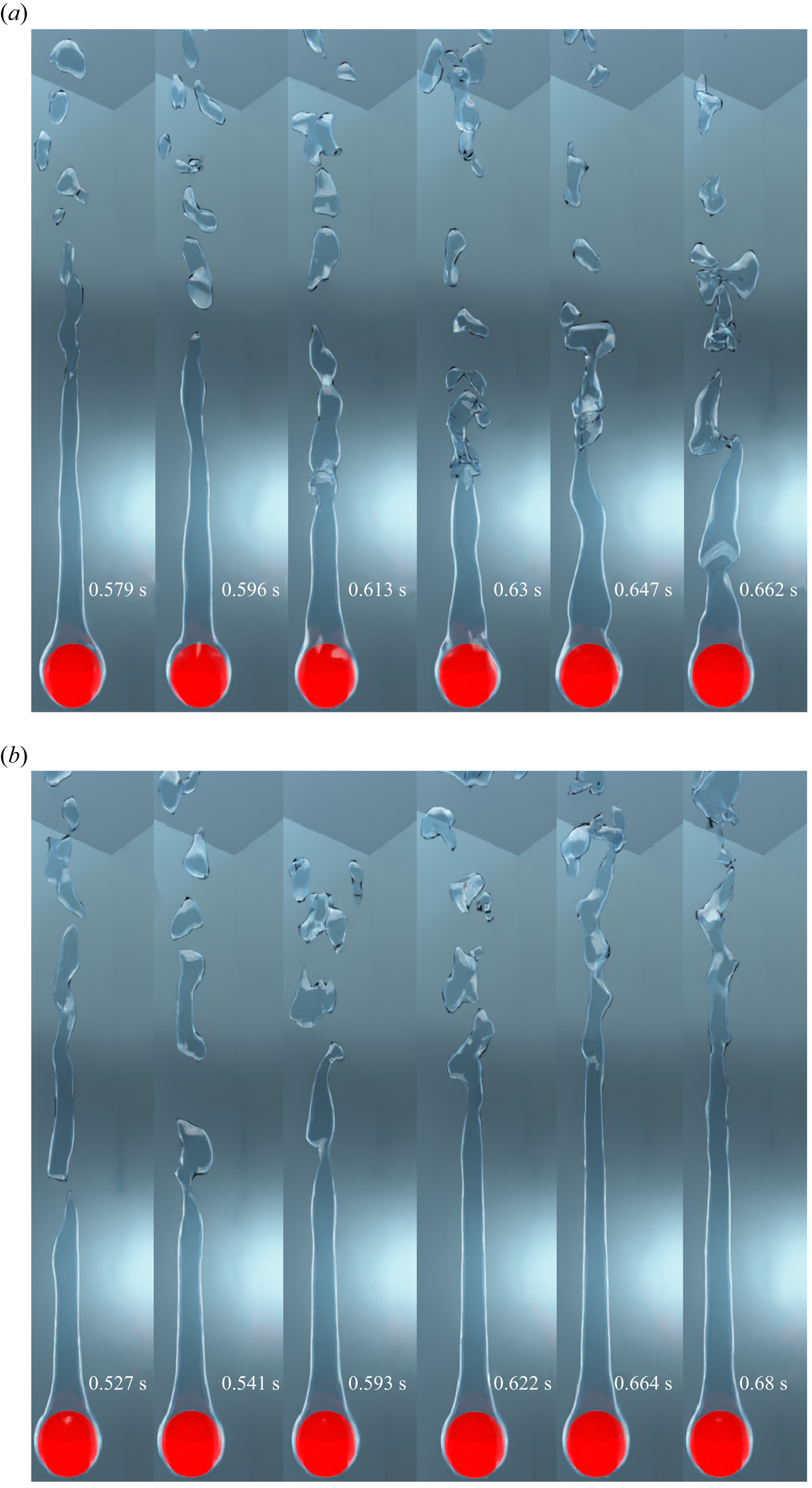
A close-up view of the thin vapour film for the case of vertical flow film boiling for  $\tilde {D}=5$ is shown in figure 14 at
 $Re_D=50$ and
 $100$. In this figure, interfacial waves can be seen on the top portion of the vapour film at different time instants. Such interfacial waves were also evident in the experimental results of Liu & Theofanous (Reference Liu and Theofanous1996). The presence of such interfacial waves implies that the vapour film thickness is not always uniform around the heated sphere for the dimensionless diameter of
 $\tilde {D}=5$. Two important inferences can be deduced from this observation, which is applicable particularly for
 $\tilde {D}=5$. Firstly, figure 14 shows that contrary to the assumption of a constant film thickness in many analytical works available in the literature, the flow in the vapour wake can be predicted accurately only if the vapour film thickness is not considered to be uniform around the sphere. Secondly, these interfacial waves tend to constantly affect the flow characteristics in the vapour film around the heated surface. Thus, the angle of separation of the vapour phase within the vapour wake seems to be a strong function of time for the dimensionless sphere diameter of
 $\tilde {D}=5$, at
 $Re_D=50$ and
 $100$.
Zoomed view of the thin vapour layer around the sphere for  $\tilde {D}=5$ and
 ${Ja^*}=0.6$ at
 $Re_D=50$ and
 $100$. Results are shown for (a)
 $Re_D=50$,
 $\sqrt {Fr}=0.05$; (b)
 $Re_D=100$,
 $\sqrt {Fr}=0.1$.

Interface evolution for the vertical flow film boiling on the dimensionless sphere diameter of  $\tilde {D}=0.5$ is shown in figure 15 for
 ${Ja^*}=0.6$. The pattern of interface evolution for
 $\tilde {D}=0.5$ is quite similar to the interface evolution for
 $\tilde {D}=1$, which has been presented in § 4.1. The vapour bubble evolves periodically at
 $Re_D=50$. However, the vapour bubble diameter
 $(D_{vb})$ at the instant of departure from the vapour film is more for
 $\tilde {D}=0.5$ than
 $\tilde {D}=1$, at
 $Re_D=50$ for the vertical flow configuration. At
 $Re_D=50$,
 $D_{vb}$ is
 $2.425D$ and
 $1.902D$ for
 $\tilde {D}=0.5$ and
 $\tilde {D}=1$, respectively. Here, for
 $\tilde {D}=0.5$, the inertial and buoyancy forces must overcome the strong surface tension force before the bubble is released in the wake region of the sphere for the mixed and forced convection film boiling. This leads to more vapour accumulating before the vapour bubble detaches from the film. The former reasoning is supported further by the small Grashof number for
 $\tilde {D}=0.5$, which indicates the dominance of viscous force over the buoyancy force. Hence, the diameter of the vapour bubble at departure is expected to rise with a decrease in
 $\tilde {D}$. An increase in Reynolds number leads to the formation of a stable vapour column in the wake region of the sphere. The vapour column thickness, with respect to the diameter of the sphere, is more for
 $\tilde {D}=0.5$ than
 $\tilde {D}=5$ for the same Reynolds number. This indicates that the angle of separation in the vapour wake increases as
 $\tilde {D}$ increases.
Interface evolution for the vertical flow configuration for  $\tilde {D}=0.5$ and
 ${Ja^*}=0.6$ at
 $Re_D$ of
 $50$ and
 $300$. Results are shown for (a)
 $Re_D=50$,
 $\sqrt {Fr}=1.7$; (b)
 $Re_D=300$,
 $\sqrt {Fr}=10.25$.

Interface evolution for the horizontal flow film boiling on a large-diameter sphere of  $\tilde {D}=5$ is shown in figure 16 for
 ${Ja^*}=0.6$ and
 $Re_D=300$. As observed in the vertical flow configuration, a vapour column is seen to develop in the wake region of the sphere. However, the vapour column is inclined towards the flow direction owing to the combined effect of the inertial and buoyancy forces for the horizontal flow configuration. The vapour column is observed to be quite unstable in the horizontal flow configuration, as shown in figure 16 as opposed to the vertical flow configuration. The vapour column oscillates under the combined influence of buoyancy and inertial forces, which results in the release of random vapour bubbles downstream of the sphere. Another significant observation is that the undulations in the vapour film near the sphere are less for the horizontal flow configuration as compared with the vertical flow configuration. Surprisingly, the single vapour column is seen to split and form two smaller columns for a very short duration, which eventually merge with each other again to form a single vapour column, as illustrated in figure 16 at time
 $t=0.467$ and
 $0.492\ \textrm {s}$.
Interface evolution for the horizontal flow configuration for  $\tilde {D}=5$ and
 ${Ja^*}=0.6$ at
 $Re_D=300$,
 $\sqrt {Fr}=0.3$.
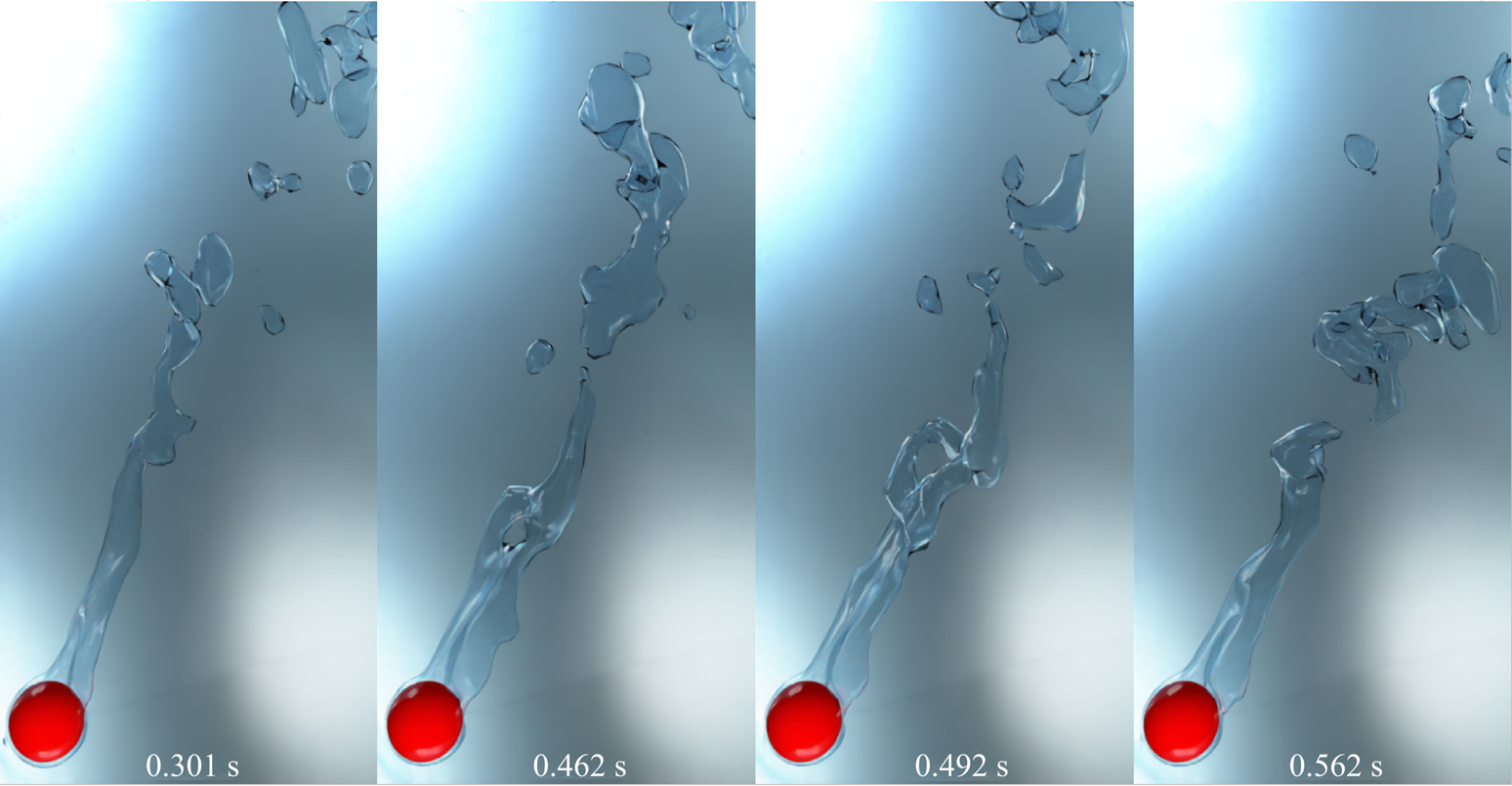
A zoomed view of the vapour column for the horizontal flow film boiling configuration for  $\tilde {D}=5$ and
 $Re_D=300$ is shown in figure 17 in two different views. In this case, the vapour column is always inclined towards the flow direction at all times. In the first view of figure 17, a vapour sheet is observed to grow beside the vapour column at time
 $t=0.212\ \textrm {s}$. This vapour column is seen to elongate during the time
 $t=0.337\mbox{--}0.416\ \textrm {s}$. Another intriguing feature is that the distance between the bottom of the vapour sheet and the heated sphere fluctuates continually as the vapour is formed in the thin film region surrounding the heated sphere and is supplied to the vapour column under the combined influence of the inertia and buoyancy forces. According to the second view of figure 17, in reality, a cusp-like structure develops parallel to the vapour column, which demonstrates a complicated interplay between the inertia, buoyancy and the surface tension forces for
 $\tilde {D}=5$.
Zoomed views of the evolving interface for the horizontal flow film boiling on a sphere for  $\tilde {D}=5$ and
 ${Ja^*}=0.6$ at
 $Re_D=300$,
 $\sqrt {Fr}=0.3$. (a) First view and (b) second view.

The interface evolution for  $\tilde {D}=0.5$ is shown in figure 18 for
 $Re_D=50$ and
 $300$ at
 ${Ja^*}=0.6$. The interface evolution for
 $\tilde {D}=1$ and the same
 ${Ja^*}$ is presented in § 4.1 for different Reynolds numbers. At
 $Re_D=50$, the vapour bubble evolves periodically for
 $\tilde {D}=0.5$. However, the vapour bubble evolution pattern is not similar to that of
 $\tilde {D}=1$, as a vapour recoil towards the heated surface and successive undulations in the thin vapour film are completely absent owing to the strong influence of the inertial force for
 $\tilde {D}=0.5$ as compared with that of
 $\tilde {D}=1$. Additionally, the vapour wake is more elongated along the flow direction, which reaffirms the dominance of the inertial force for
 $\tilde {D}=0.5$ as compared with that of
 $\tilde {D}=1$ for the same Reynolds number. A dominant surface tension force in the case of
 $\tilde {D}=0.5$ as compared with that of
 $\tilde {D}=1$ leads to the formation of a comparatively larger vapour bubble at pinch-off. For
 $Re_D=50$,
 $D_{vb}$ is
 $3.204D$ and
 $2.041D$ at
 $\tilde {D}=0.5$ and
 $\tilde {D}=1.0$, respectively. Furthermore, the pinch-off location is significantly relocated downstream of the heated sphere. In addition to this, a steady vapour wake is created along the flow direction as shown in figure 18(a) at time
 $t=0.393\mbox{--}0.521\ \textrm {s}$, with the constant-sized vapour bubbles being torn away from the tail of the wake. An important observation in the case of
 $\tilde {D}=0.5$ at
 $Re_D=50$ is that the thin vapour layer uniformly covers the left half of the heated sphere, unlike the case of
 $\tilde {D}=1$, as there is no vapour bulge in the lower-right portion of the heated sphere for
 $\tilde {D}=0.5$. The interface evolution for a small diameter sphere
 $(\tilde {D}=0.5)$ at
 $Re_D=300$ is shown in figure 18(b). In this figure a vapour column is formed in the wake of the sphere, which tends to oscillate under the action of strong inertial force at
 $Re_D=300$. For
 $\tilde {D}=0.5$ and
 $Re_D=300$, a thin vapour film uniformly covers the left half of the sphere for the horizontal flow configuration. Thus, it can be concluded that for the horizontal flow configuration, the thin vapour film uniformly covers the left half of the heated sphere for both
 $\tilde {D}=0.5$ and
 $1$ at high Reynolds numbers. However, the thickness of the vapour film at
 $Re_D=300$ is significantly less at
 $\tilde {D}=0.5$ as compared with that of
 $\tilde {D}=1$ owing to the presence of a strong surface tension force for
 $\tilde {D}=0.5$. In addition to this, the curved surface area covered by the thin vapour film keeps changing for
 $\tilde {D}=0.5$ as seen in figure 18(b) for time instants
 $t=0.496, 0.536, 0.711\ \textrm {s}$ as compared with
 $\tilde {D}=1$. This illustrates that the angle of separation within the vapour wake varies for the dimensionless sphere diameter of
 $\tilde {D}=0.5$ in the horizontal flow film boiling.
Interface evolution for the horizontal flow configuration for  $\tilde {D}=0.5$ and
 ${Ja^*}=0.6$ at different
 $Re_D$. Results are shown for (a)
 $\tilde {D}=0.5$,
 $Re_D=50$,
 $\sqrt {Fr}=1.7$; (b)
 $\tilde {D}=0.5$,
 $Re_D=300$,
 $\sqrt {Fr}=10.25$.

The variation of  $\tau _v/D$ with
 $\tilde {D}$ at
 ${Ja^*}=0.6$ and different
 $Re_D$ is shown in figure 19 for both the vertical and horizontal flow configurations. For all
 $Re_D$,
 $\tau _v/D$ increases as
 $\tilde {D}$ increases. However, the percentage change in
 $\tau _v/D$ is very small as the
 $\tilde {D}$ increases from
 $1$ to
 $5$ as compared with the case when
 $\tilde {D}$ increases from
 $0.5$ to
 $1$.
Variation of  $\tau _v/D$ vs
 $\tilde {D}$ at different
 $Re_D$ at
 ${Ja^*}=0.6$ for both the vertical and horizontal flow configurations.
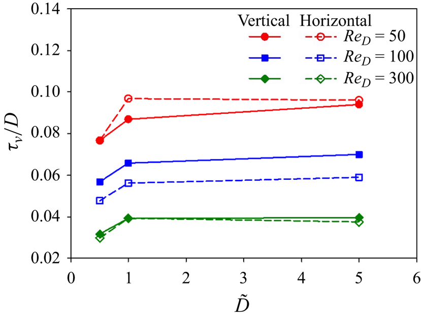
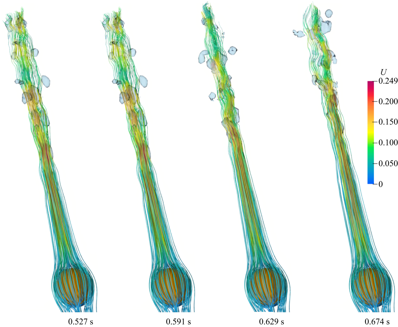
Figure 20 shows the 3-D streamlines in the vapour wake for the vertical flow film boiling for  $\tilde {D}=5$ and
 $Re_D=300$ at
 ${Ja^*}=0.6$. This figure shows that the vapour column in the wake region of the sphere results in closer 3-D streamlines, which indicate high velocity in that region. This can be supported by the argument that the formation of a vapour column in the wake region often restricts the vapour flow to a very narrow region. Thus, the vapour velocity is seen to increase in the column downstream of the heated surface. The 3-D streamlines are seen to bend and diverge after the tail of the vapour column, owing to a very random and chaotic motion of the released vapour bubbles.
Three-dimensional streamlines within the vapour wake for the vertical flow configuration at  $Re_D=300$,
 $\sqrt {Fr}=0.3$ for
 $\tilde {D}=5$ and
 ${Ja^*}=0.6$.
The 3-D streamlines for the case of vertical flow film boiling on a dimensionless diameter of  $\tilde {D}=0.5$ at
 $Re_D=300$ and
 ${Ja^*}=0.6$ are shown in figure 21. As shown in this figure, a recirculation region is seen to develop within the vapour phase in the vapour wake. This recirculation region is elongated along the flow direction along with the vapour phase. A comparison of the 3-D streamlines shown in figure 21 at
 $t=0.11$ s and 0.15 s indicates that the recirculation regions have attained a constant size, although the vapour phase continues to elongate along the flow direction. For
 $\tilde {D}=0.5$ at
 $Re_D=300$ and
 ${Ja^*}=0.6$,
 $\theta _s$ is measured to be
 $110.93^{\circ }$. The separation angle for the same
 $Re_D$ and
 ${Ja^*}$ at
 $\tilde {D}=1$ is
 $114.84^{\circ }$. Thus, this observation again reaffirms our previous observation that the separation angle increases as
 $\tilde {D}$ increases for a fixed
 $Re_D$ and
 ${Ja^*}$.
Three-dimensional streamlines within the vapour wake for the vertical flow configuration at  $Re_D=300$,
 $\sqrt {Fr}=10.25$ for
 $\tilde {D}=0.5$ and
 ${Ja^*}=0.6$.

The instantaneous 3-D streamlines for the horizontal flow film boiling configuration for  $\tilde {D}=0.5$ are shown in figure 22 for
 $Re_D=50$ and
 $300$, respectively, at
 ${Ja^*}=0.6$. As shown in figure 22(a), the streamlines bend abruptly just after the pinch-off of the vapour bubble at time
 $t=0.626$ and
 $0.656\ \textrm {s}$. However, the absence of the vapour recoil towards the heated surface prevents the formation of recirculations in the vapour wake, as was observed in the case of
 $\tilde {D}=1$. This is due to the combined effect of the surface tension and the inertial forces for
 $\tilde {D}=0.5$. Recirculations can be seen in the vapour wake at all times for
 $\tilde {D}=0.5$ and
 $Re_D=300$ as shown in figure 22(b). The size of these recirculations continuously changes with time. These observations point to a complex connection between the liquid and vapour wake for
 $\tilde {D}=0.5$ at
 $Re_D=300$. In the case of
 $\tilde {D}=5$, the streamlines are uniformly distributed around the heated spherical surface as shown in figure 23. This confirms the presence of a thin vapour film, which covers the heated surface uniformly. In the vapour phase, the vapour velocity is large, and the streamlines are closer to each other. The 3-D streamlines are seen moving away from each other when the vapour column starts disintegrating into small random-sized vapour bubbles. Furthermore, as seen in figure 23, the streamlines incur severe deformation even in the liquid wake for
 $\tilde {D}=5$ at
 $Re_D=300$. This observation again reinforces a strong coupled interaction between the liquid and vapour wake, even for
 $\tilde {D}=5$ in the horizontal flow configuration.
Three-dimensional streamlines within the vapour wake for the horizontal flow configuration for  $\tilde {D}=0.5$ at different
 $Re_D$ for
 ${Ja^*}=0.6$. Results are shown for (a)
 $Re_D=50$,
 $\tilde {D}=0.5$,
 $\sqrt {Fr}=1.7$; (b)
 $Re_D=300$,
 $\tilde {D}=0.5$,
 $\sqrt {Fr}=10.25$.
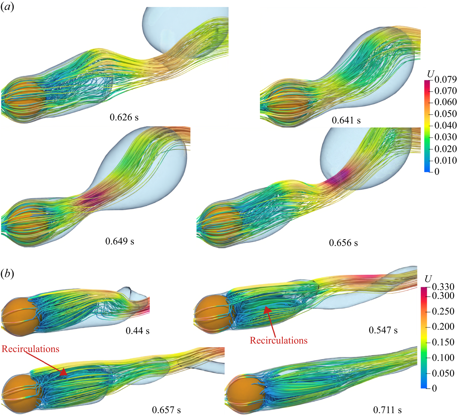
Three-dimensional streamlines within the vapour wake for the horizontal flow configuration for  $\tilde {D}=5$ at
 $Re_D=300$,
 $\sqrt {Fr}=0.3$ and
 ${Ja^*}=0.6$.
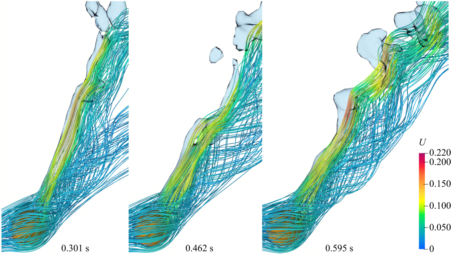
The temporal variation of the  $Nu_{spaceAvg}$ for both the vertical and horizontal flow configuration is shown in figures 24(a)–24(d) for a sphere of dimensionless diameter
 $\tilde {D}=0.5$ and
 $\tilde {D}=5$, at
 ${Ja^*}=0.6$. For the vertical flow configuration,
 $Nu_{spaceAvg}$ varies periodically for
 $\tilde {D}=0.5$. However, as the
 $Re_D$ increases, the time period of the vapour bubble ebullition cycle increases for
 $Re_D=100$. Furthermore, the difference between the minimum and maximum values of
 $Nu_{spaceAvg}$, once it starts varying periodically, decreases as the Reynolds number is increased. As shown in figure 24(a), the fluctuation in the
 $Nu_{spaceAvg}$ is insignificant at
 $Re_D=200$ and
 $300$. As shown in figure 24(b), for the case of vertical flow film boiling for
 $\tilde {D}=5$, the
 $Nu_{spaceAvg}$ is constant. This can be due to the long vapour column in the wake region of the sphere for all Reynolds numbers.
Nusselt numbers for  $\tilde {D}=0.5$ and
 $5$ at different
 $Re_D$ and
 ${Ja^*}=0.6$. Plots of (a,b)
 $Nu_{spaceAvg}$ versus time for
 $\tilde {D}=0.5$ and
 $5$ for different
 $Re_D$ for vertical flow, (c,d)
 $Nu_{spaceAvg}$ versus time for
 $\tilde {D}=0.5$ and
 $5$ for different
 $Re_D$ for horizontal flow, (e)
 $Nu_{timeAvg}$ vs
 $\tilde {D}$ for different
 $Re_D$.
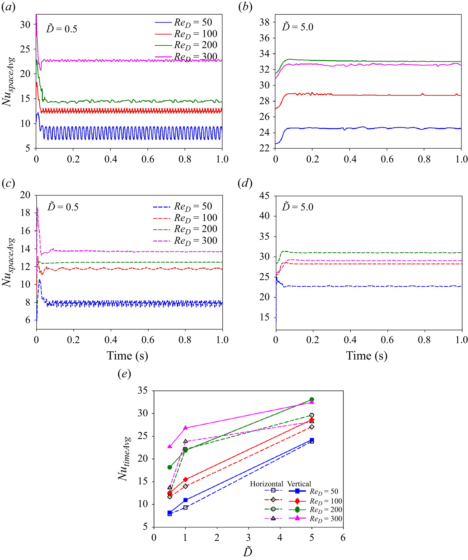
As shown in figure 24(c), for the horizontal flow film boiling configuration for  $\tilde {D}=0.5$, the
 $Nu_{spaceAvg}$ varies periodically at
 $Re_D=50$ and
 $100$. At
 $Re_D=100$, the time period of the vapour bubble ebullition cycle increases compared with
 $Re_D=50$ for
 $\tilde {D}=0.5$. At higher Reynolds numbers of
 $Re_D=200$ and
 $300$ for
 $\tilde {D}=0.5$, the
 $Nu_{spaceAvg}$ is nearly constant. This is due to the presence of a stable and uniform thin vapour film that covers a major curved surface area of the heated sphere. Furthermore, the random fluctuations in the vapour wake caused by the external flow field have the least effect on the
 $Nu_{spaceAvg}$. For
 $\tilde {D}=5$, as shown in figure 24(d), the
 $Nu_{spaceAvg}$ eventually becomes constant. This is due to the long vapour column in the wake region of the sphere.
The variation of  $Nu_{timeAvg}$ with
 $\tilde {D}$ is shown in figure 24(e) at
 ${Ja^*}=0.6$. It is observed that for both flow configurations,
 $Nu_{timeAvg}$ increases with
 $\tilde {D}$ for a fixed
 $Re_D$. However,
 $Nu_{timeAvg}$ does not increase in direct proportion to
 $\tilde {D}$. Therefore, the heat transfer coefficient decreases as
 $\tilde {D}$ increases for both the vertical and horizontal flow configurations. In the vertical flow configuration, for example, at
 $Re_D=100$, a change in
 $\tilde {D}$ from
 $0.5$ to
 $1$ increases
 $Nu_{timeAvg}$ by
 $23\,\%$, while a change in
 $\tilde {D}$ from
 $1$ to
 $5$ increases it by
 $85\,\%$. A similar trend is also observed for the horizontal flow configuration. This implies that the heat transfer decreases as the dimensionless sphere diameter increases for both flow configurations. As shown in figure 24(e),
 $Nu_{timeAvg}$ decreases for
 $Re_D=300$ and
 $\tilde {D}=5$ for horizontal flow. As shown in figure 17, the presence of a cusp-shaped structure along the vapour column at
 $Re_D=300$ tends to restrict the flow of vapour into the vapour column, thus raising the temperature of the vapour trapped inside the thin film and results in a low heat transfer coefficient.
4.3. Effect of dimensionless wall superheat
The effect of dimensionless wall superheat on the heat transfer and the associated flow characteristics in the liquid and vapour wake for the flow film boiling on a heated sphere is investigated in detail in this section. In this regard, in order to understand the effect of wall superheat on the interface evolution, the results corresponding to three different values of  ${Ja^*}$ of
 $0.3, 0.6$ and
 $0.9$ are presented in this work for
 $Re_D=50$ and
 $\tilde {D}=1$.
Figure 25 shows the temporal evolution of the interface for the vertical flow film boiling configuration for  $\tilde {D}=1$ and
 $Re_D=50$ at
 ${Ja^*}=0.3$ and
 $0.9$. As shown in figure 25, for both
 ${Ja^*}=0.3$ and
 $0.9$ at
 $Re_D=50$, the vapour bubble evolves periodically. In these cases, vapour gets continuously generated in the thin vapour region and accumulates on the top of the heated spherical surface due to the buoyancy force and is released once it has attained a certain size. However, it is clear from figure 25 that as
 ${Ja^*}$ increases, the tail of the vapour wake elongates along the flow direction and the vapour bubbles are released far downstream the sphere, in the vertical flow configuration. This observation is consistent with the experimental results of Reimann & Grigull (Reference Reimann and Grigull1975). An increase in vapour film thickness around the sphere is also evident as
 ${Ja^*}$ increases due to the increased vapour generation under the same external flow conditions. Additionally, when
 ${Ja^*}$ increases, the bubble release frequency also increases for the vertical flow configuration. In addition to this,
 $D_{vb}$ was calculated for
 $\tilde {D}=1$ and
 $Re_D=50$ at
 ${Ja^*}=0.3$ and
 $0.9$. For these conditions,
 $D_{vb}$ is
 $1.815D$ and
 $2.019D$ at
 ${Ja^*}=0.3$ and
 $0.9$, respectively. Thus, it is clear that
 $D_{vb}$ increases with
 ${Ja^*}$ due to more vapour generation at higher
 ${Ja^*}$.
Interface evolution for the vertical flow configuration for  $\tilde {D}=1$ and
 $Re_D=50$,
 $\sqrt {Fr}=0.6$ at different wall superheats. Results are shown for (a)
 ${Ja^*}=0.3$ and (b)
 ${Ja^*}=0.9$.

The 3-D streamlines inside the vapour in the wake of the sphere are shown in figure 26 for  $\tilde {D}=1$,
 $Re_D=50$ and
 ${Ja^*}=0.3$ and
 $0.9$. Recirculations are observed within the growing vapour bubble near the rear stagnation point. However, a considerable reduction in the recirculations is observed as the
 ${Ja^*}$ increases. This can be due to more vapour generation at
 ${Ja^*}=0.9$, which results in an elongated vapour wake downstream of the sphere. A visual comparison of figures 26(a) and 26(b) at time
 $0.623 \textrm {s}$ and
 $0.239\ \textrm {s}$, respectively, indicates that recirculations are developed within the vapour phase just after the vapour bubble is released and the interface tends to recoil towards the sphere. However, it should be noted that the size of these recirculations behind the sphere is smaller for
 ${Ja^*}=0.9$ than that of
 ${Ja^*}=0.3$. Also, the flow velocity within the vapour phase increases with
 ${Ja^*}$.
Three-dimensional streamlines within the vapour wake for the vertical flow configuration for  $\tilde {D}=1$ at
 $Re_D=50$,
 $\sqrt {Fr}=0.6$ at different wall superheats. Results are shown for (a)
 ${Ja^*}=0.3$ and (b)
 ${Ja^*}=0.9$.
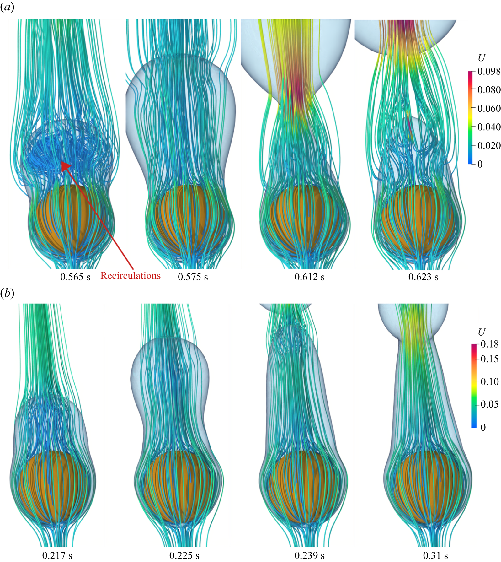
The temperature distribution within the vapour bubble is presented in figure 27 for  $\tilde {D}=1$ and
 $Re_D=50$ at
 ${Ja^*}=0.3$ and
 ${Ja^*}=0.9$ for the vertical flow configuration. The maximum temperature within the departed vapour bubble increases with an increase in
 ${Ja^*}$. As shown in figure 27(a), the vapour bubble is released at time
 $0.211\ \textrm {s}$. Thereafter, under the effect of the surface tension force, the interface tends to recoil back towards the heater surface from
 $0.211\ \textrm {s}$ to
 $0.215\ \textrm {s}$. During this recoil motion of the interface, a high temperature is observed in the central region of the vapour mass as seen at time
 $0.211\ \textrm {s}$. Moreover, as the interface begins to recoil back towards the sphere, the temperature within the core of the vapour mass starts falling until time
 $0.215\ \textrm {s}$. After this time instant, the bubble ebullition cycle gets repeated. On the contrary, for
 ${Ja^*}=0.9$, the temperature within the central region of the vapour mass is uniform, even during the vapour recoil motion as shown in figure 27(b) at time
 $0.218\ \textrm {s}\mbox{--}0.220\ \textrm {s}$. This observation can be attributed to a very short duration of vapour recoil motion due to high vapour generation at
 ${Ja^*}=0.9$.
Temperature distribution within the vapour for  $\tilde {D}=1$ at
 $Re_D=50$,
 $\sqrt {Fr}=0.6$ at different wall superheats. Results are shown for (a)
 ${Ja^*}=0.3$ and (b)
 ${Ja^*}=0.9$.
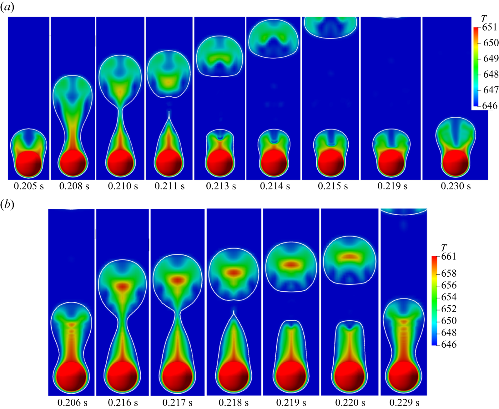
The interface evolution for the horizontal flow film boiling configuration for  $\tilde {D}=1$ and
 ${Ja^*}=0.3$ and
 $0.9$ at
 $Re_D=50$ is shown in figure 28. Vapour is continuously generated in the thin film region, and it tends to gather in the top-right region of the sphere from where the vapour bubble is periodically shed. For
 ${Ja^*}=0.3$ and
 ${Ja^*}=0.9$,
 $D_{vb}$ is
 $1.978D$ and
 $2.201D$, respectively. Therefore, as shown in figure 28, the size of the vapour bubbles increases as
 ${Ja^*}$ increases for the horizontal flow configuration. This is due to the fact that the volume of the vapour produced at
 ${Ja^*}=0.9$ is substantially higher than that at
 ${Ja^*}=0.3$. Furthermore, because of the formation of a stable vapour column at the dimensionless wall superheat of
 ${Ja^*}=0.9$, the vapour bubbles are released far from the sphere as shown in figure 28(b) at time
 $t=0.435\ \textrm {s}$. Another intriguing feature is that even if the vapour bubbles are released into the wake region of the sphere periodically at a dimensionless wall superheat of
 ${Ja^*}=0.9$, the residual vapour mass does not recoil towards the sphere. Given the same flow conditions, this demonstrates that the surface tension force is dominated by the buoyancy force at
 ${Ja^*}=0.9$ for the horizontal flow configuration. In addition to this, as shown in figure 28(a), the location of bubble pinch-off is fixed in the case of
 ${Ja^*}=0.3$. However, at
 ${Ja^*}=0.9$, after the first vapour bubble pinch-off, the next vapour bubble grows and elongates along the flow direction and pinches off as shown in figure 28(b) at times
 $t=0.114, 0.32$ and
 $0.347\ \textrm {s}$. The 3-D streamlines within the vapour wake for the horizontal flow configuration for
 $\tilde {D}=1.0$ at
 $Re_D=50$ and
 ${Ja^*}=0.3$ and
 $0.9$ are shown in figure 29. The number of recirculations has dropped significantly as
 ${Ja^*}$ has increased. This is because the vapour bubbles are released further downstream of the heated sphere and also due to the absence of vapour mass recoil towards the heated sphere after the bubble pinch-off. In addition to this, the velocity within the vapour phase has increased as
 ${Ja^*}$ is increased from
 $0.3$ to
 $0.9$.
Interface evolution for the horizontal flow configuration for  $\tilde {D}=1$ and
 $Re_D=50$,
 $\sqrt {Fr}=0.6$ at different wall superheats. Results are shown for (a)
 ${Ja^*}=0.3$ and (b)
 ${Ja^*}=0.9$.
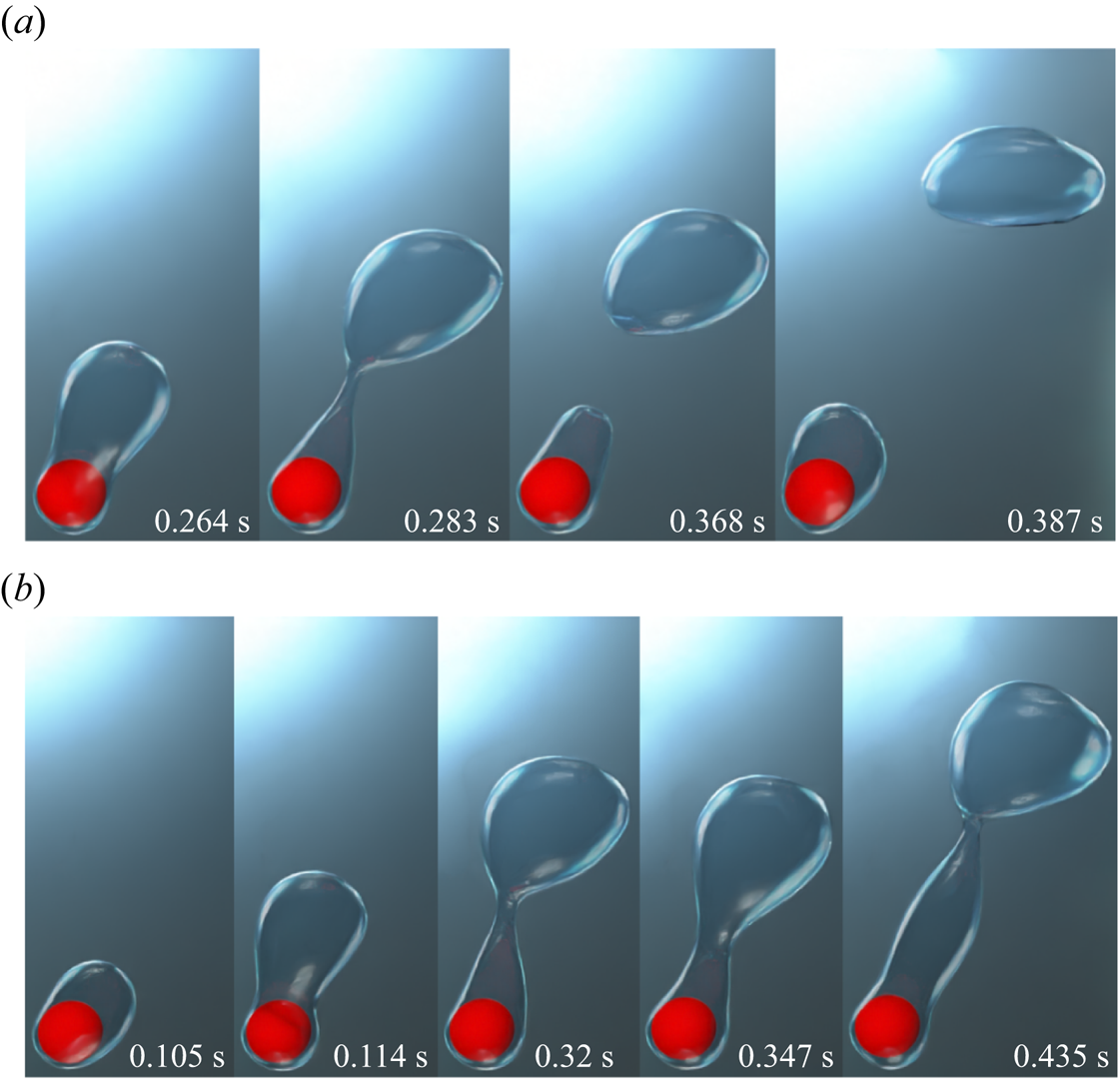
Three-dimensional streamlines within the vapour wake for the horizontal flow configuration for  $\tilde {D}=1$ at
 $Re_D=50$,
 $\sqrt {Fr}=0.6$ at different wall superheats. Results are shown for (a)
 ${Ja^*}=0.3$ and (b)
 ${Ja^*}=0.9$.
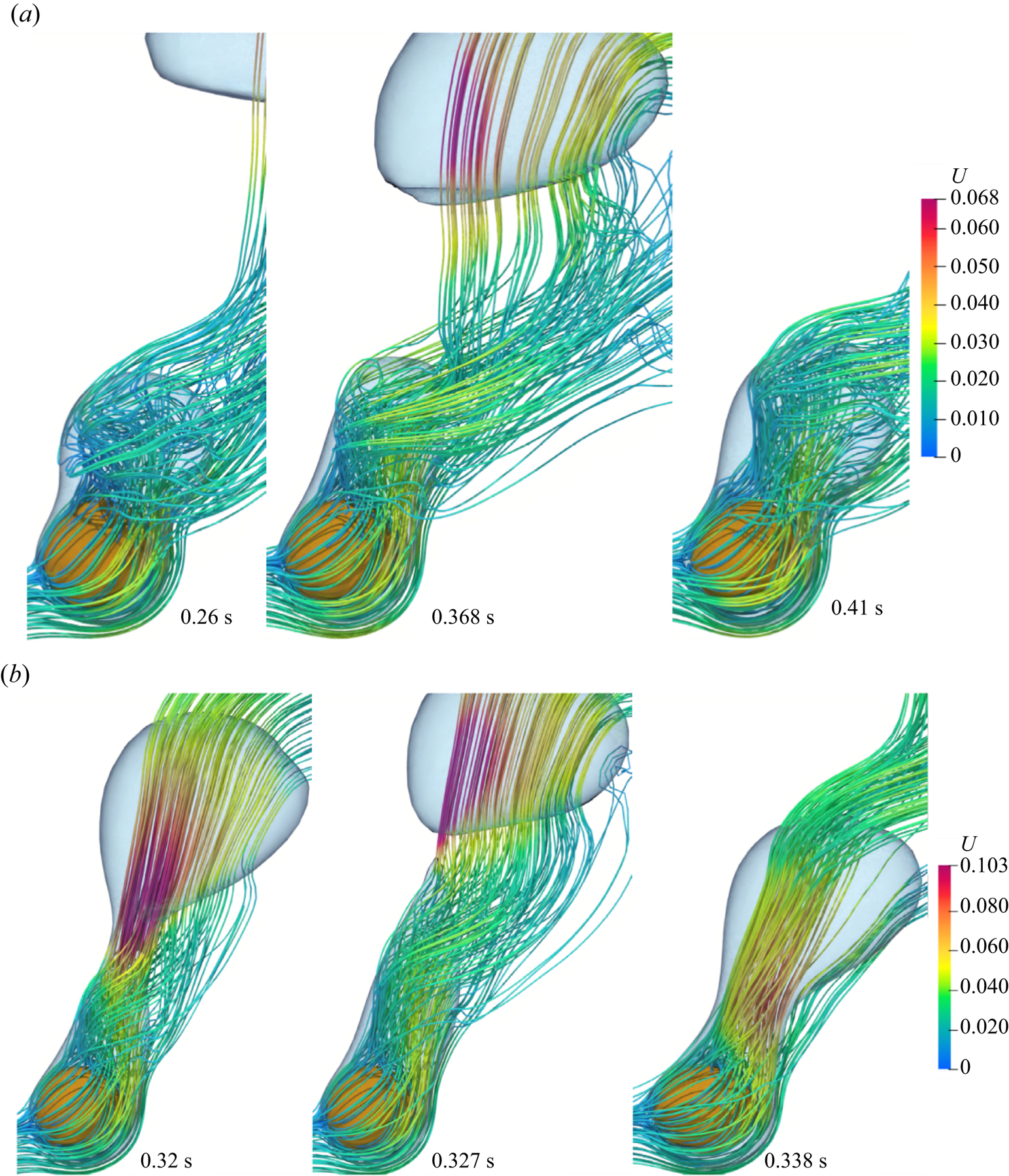
The temperature distribution within the vapour bubble is presented in figure 31 for  $\tilde {D}=1$ and
 $Re_D=50$ at
 ${Ja^*}=0.3$ and
 ${Ja^*}=0.9$, for the horizontal flow configuration. In the horizontal flow configuration, a high-temperature region is observed near the top-right region of the sphere at all times and for all the values of dimensionless wall superheat. For the low dimensionless wall superheat of
 ${Ja^*}=0.3$, a thermal plume (with temperature ranging between 650–651 K) is evident near the top-right region of the sphere at time
 $0.283\ \textrm {s}$. However, the height of this thermal plume decreases during the vapour recoil motion as shown in figure 31(a) at time
 $0.286\mbox{--}0.292\ \textrm {s}$. As shown in figure 31(b), a similar thermal plume (with temperature ranging between 658–661 K) is also evident at time
 $0.225\mbox{--}0.234\ \textrm {s}$ for
 ${Ja^*}=0.9$. However, contrary to the case of
 ${Ja^*}=0.3$, the height of the thermal plume is higher for
 ${Ja^*}=0.9$. This again reinforces the observation of a very short-duration vapour recoil towards the heated surface at a high dimensionless wall superheat of
 $0.9$. For
 ${Ja^*}=0.9$ at
 $0.238\ \textrm {s}$, as soon as the interface recoil motion ends and the formation of a new vapour bubble starts, the thermal plume (as observed in the case of
 ${Ja^*}=0.3$) completely disappears. A high-temperature region can be seen in the central core of the vapour mass near the top-right region of the heated sphere at time 0.238 s in figure 31(b).
The variation of  $\tau _v/D$ with
 ${Ja^*}$ at
 $\tilde {D}=1$ and
 $Re_D=50$ is shown in figure 30 for both the vertical and horizontal flow configurations. For both flow configurations,
 $\tau _v/D$ increases as
 ${Ja^*}$ increases. This can be due to the increased vapour generation at a higher dimensionless wall superheat. Here
 $\tau _v/D$ is more for the vertical flow configuration at
 ${Ja^*}=0.3$ as compared with the horizontal flow configuration. However, at
 ${Ja^*}=0.6$ and
 $0.9$,
 $\tau _v/D$ is more for the horizontal flow configuration as compared with the vertical flow configuration.
Variation of  $\tau _v/D$ vs
 ${Ja^*}$ at
 $\tilde {D}=1$ and
 $Re_D=50$ for both the vertical and horizontal flow configurations.
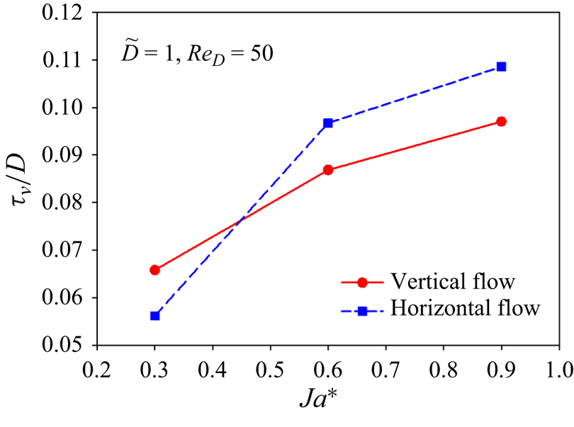
Temperature distribution within the vapour for  $\tilde {D}=1$ at
 $Re_D=50$,
 $\sqrt {Fr}=0.6$ at different wall superheats. Results are shown for (a)
 ${Ja^*}=0.3$ and (b)
 ${Ja^*}=0.9$.
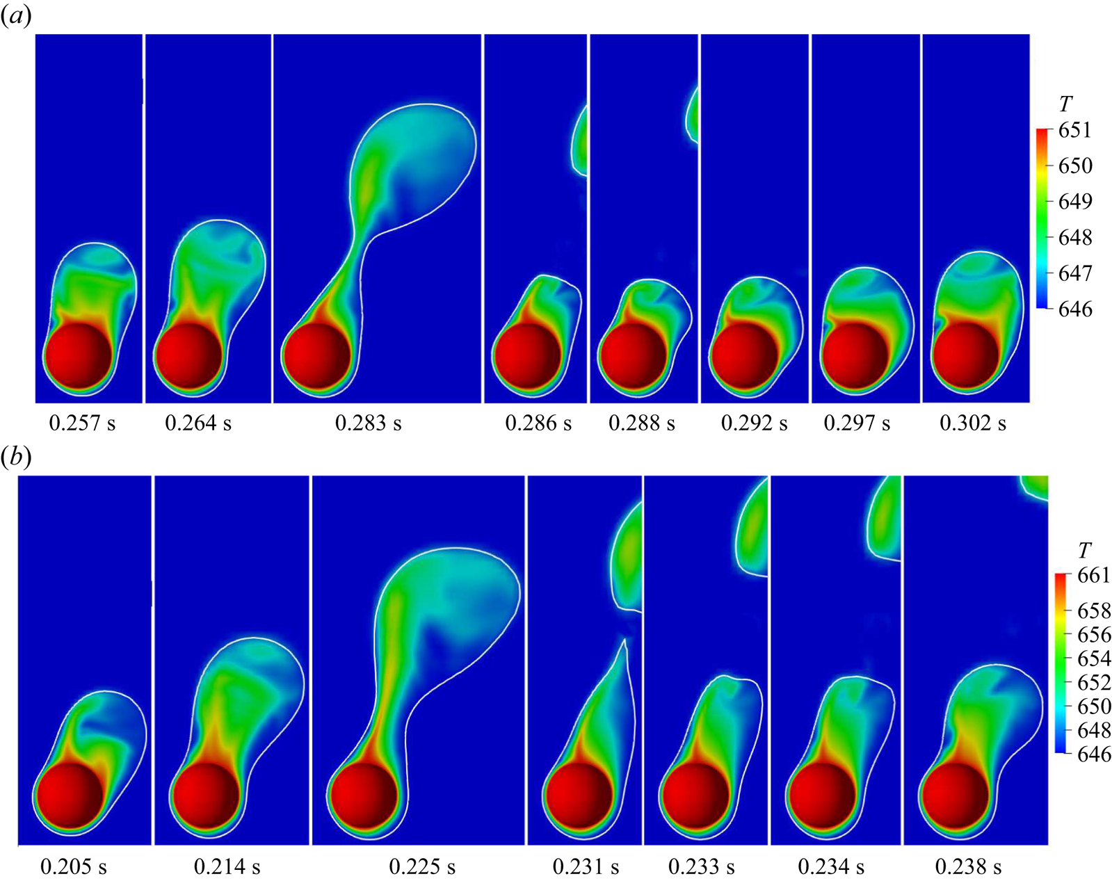
The temporal variation of  $Nu_{spaceAvg}$ is shown in figure 32 for the dimensionless wall superheats of
 $0.3$ and
 $0.9$. The
 $Nu_{spaceAvg}$ depicts periodic variation for the vertical flow configuration for
 $\tilde {D}=1$ and
 $Re_D=50$ and
 $100$ for both
 ${Ja^*}=0.3$ and
 $0.9$ as shown in figures 32(a) and 32(b). However, the time period of the variation drastically decreases as
 ${Ja^*}$ increases for
 $Re_D=100$ owing to the increased buoyancy force and greater vapour generation. The difference between the maximum and minimum values of
 $Nu_{spaceAvg}$ decreases considerably as
 ${Ja^*}$ increases for the case of
 $\tilde {D}=1$ and
 $Re_D=50$ and
 $100$ for the vertical flow configuration.
Nusselt numbers for  $\tilde {D}=1$ at various
 $Re_D$ and
 ${Ja^*}$. Plots of (a,b)
 $Nu_{spaceAvg}$ versus time for
 $\tilde {D}=1$ for different
 $Re_D$ and
 ${Ja^*}=0.3, 0.9$ for vertical flow, (c)
 $Nu_{spaceAvg}$ versus time for
 $\tilde {D}=1$ for different
 $Re_D$ and
 ${Ja^*}=0.9$ for horizontal flow, (e)
 $Nu_{timeAvg}$ vs
 $Re_D$ for
 $\tilde {D}=1$ at different
 ${Ja^*}$.

The  $Nu_{spaceAvg}$ for the horizontal flow film boiling for
 $\tilde {D}=1$ and
 ${Ja^*}=0.3$ and
 $0.9$ is shown in figures 32(c) and 32(d), respectively. As the dimensionless wall superheat increases, the difference between the maximum and minimum
 $Nu_{spaceAvg}$ decreases. This is because the vapour bubble removal process changes from isolated bubbles to the formation of a vapour column at a higher wall superheat. Figure 32(e) shows the variation of
 $Nu_{timeAvg}$ with
 $Re_D$ at different dimensionless wall superheats for both flow configurations. It can be seen that for both flow configurations,
 $Nu_{timeAvg}$ increases with
 ${Ja^*}$. However, as
 ${Ja^*}$ is increased from
 $0.3$ to
 $0.6$, the percentage change in
 $Nu_{timeAvg}$ values is much less as compared with the change when it is increased from
 $0.6$ to
 $0.9$. This percentage change in the
 $Nu_{timeAvg}$ values is different for the spheres of different dimensionless diameters.
In order to gain further insight into the heat transfer characteristics of flow film boiling on a sphere, a FFT of the  $Nu_{spaceAvg}$ is carried out in this work. The amplitude is normalized with the maximum amplitude. The FFT plots shown in figure 33 correspond to different cases of vertical flow film boiling on a sphere. The cases shown in figures 33(a)–33(c) correspond to different Reynolds numbers, while all other flow variables are fixed. In figure 33(a), at
 $Re_D=50$ and
 ${Ja^*}=0.3$, the first frequency is the most dominant frequency, and it is also the bubble release frequency. Other superharmonics are also evident, which are multiples of the bubble release frequency. This indicates that at
 $Re_D=50$, the heat transfer and the interface evolution are mostly dominated by the buoyancy force. At
 $Re_D=100$, similar to the previous case, for the same dimensionless wall superheat, the first frequency is the most dominant frequency. However, the frequency at
 $Re_D=100$ is slightly higher as compared with that at
 $Re_D=50$. It can also be seen that the other superharmonics in the case of
 $Re_D=100$ have decreased significantly in amplitude as compared with that of
 $Re_D=50$. This shows that an additional force, the inertia force, has come into play, which affects the interface evolution. This indicates that the inertial force has an appreciable effect on the interface evolution, even though the buoyancy force turns out to be the most dominant at
 $Re_D=100$. In the case of
 $Re_D=300$ and the same dimensionless wall superheat of
 ${Ja^*}=0.3$, the FFT plot is featured by two pronounced peaks, which indicates that both the buoyancy and inertial forces equally affect the heat transfer. Figures 33(a), 33(d) and 33(e) correspond to the case where only the
 ${Ja^*}$ is varied, while other parameters are kept constant. In this case, as well, the first peak corresponds to the highest normalized amplitude and turns out to be the frequency of bubble release. However, as
 ${Ja^*}$ is increased for the same Reynolds number, the amplitude of the superharmonics tends to diminish due to an appreciable increase in the buoyancy force.
The FFT of  $Nu_{spaceAvg}$ for the vertical flow configuration.

The FFT results for the horizontal flow film boiling on a sphere are shown in figure 34 for different flow conditions. The cases depicted in figures 34(a) and 34(b) correspond to the horizontal flow film boiling on a small dimensionless diameter sphere  $(\tilde {D}=0.5)$ at
 $Re_D=50$ and
 $100$. As discussed earlier, the interface evolution for
 $\tilde {D}=0.5$ is periodic at
 $Re_D=50$. The FFT plot shown in figure 34(a) reflects this as the most dominant frequency that exactly matches the frequency of bubble release. However, superharmonics can also be seen that are an exact multiple of the most dominant frequency. Furthermore, the presence of three dominant peaks in the FFT plot reveals that inertia, buoyancy and surface tension forces together influence the flow features for the horizontal flow film configuration at
 $\tilde {D}=0.5$. At
 $Re_D=100$, the superharmonics have been suppressed. However, a single most dominant frequency is present. This shows the increased influence of the inertial force over the buoyancy and surface tension force as the Reynolds number is increased. The FFT plots shown in figures 34(c) and 34(e) for
 $\tilde {D}=1$ tend to give a similar conclusion when only the Reynolds number is varied while all the other parameters are kept constant. However, for
 $\tilde {D}=1$, the frequency of the most prominent amplitude has decreased significantly as compared with that of
 $\tilde {D}=0.5$. This suggests that the combined inertia and buoyancy forces have largely negated the influence of the surface tension force for
 $\tilde {D}=1$ for the horizontal flow configuration. Figures 34(c) and 34(d) illustrate the FFT plots for different
 ${Ja^*}$, while all the other variables remain unchanged. As
 ${Ja^*}$ increases, a number of subharmonics arise while the amplitude of different superharmonics is observed to increase.
The FFT of  $Nu_{spaceAvg}$ for the horizontal flow configuration.

5. Conclusion
In the present work, both vertical and horizontal flow film boiling over a stationary heated sphere has been studied numerically using the CLSVOF method for interface capturing. For both the horizontal and vertical flow film boiling, the Reynolds number is varied from  $50$ to
 $300$, while the dimensionless wall superheat
 $({Ja^*})$ is varied between
 $0.3$ and
 $0.9$. The spheres of three different dimensionless diameters
 $(\tilde {D})$ viz.
 $0.5, 1, 5$ were considered for the investigation. In this study, a detailed investigation of the effect of these flow and geometric parameters on the interface evolution, the associated flow features and the heat transfer is carried out. Some of the main observations in this study pertaining to both the horizontal and vertical flow film boiling on a sphere are summarized as follows.
The vapour bubble evolves periodically for both the vertical and horizontal flow configurations at  $Re_D=50$ and
 $100$. A further increase in
 $Re_D$ for the same dimensionless wall superheat and sphere diameter tends to increase the length of the vapour wake along the flow direction. This reflects the relative dominance of the inertial force over the buoyancy force. For the vertical flow film boiling at
 $Re_D=200$ and
 $300$, a vapour column is seen to form along the flow direction. However, for the horizontal flow configuration at
 $Re_D=200$ and
 $300$, the vapour column fluctuates due to the surrounding liquid wake. As a result, the vapour bubbles are released randomly from the extended vapour column. For the vertical flow film boiling at
 $Re_D=50$ and
 $100$, recirculations are periodically formed and shed in the wake region while, for
 $Re_D=300$, recirculations of constant size are seen to develop within the vapour wake. The recirculations get elongated along the flow direction as the
 $Re_D$ is increased while all other parameters are kept constant for the vertical flow configuration. The extent of these recirculations was seen to significantly increase for the horizontal flow configuration at
 $Re_D=50$. For the horizontal flow configuration at
 $Re_D=50$, the vapour bubbles are released along the diagonal direction. However, for
 $Re_D=300$, the vapour wake is completely transferred to the rear of the sphere.
The effect of the dimensionless sphere diameter was also investigated in this work. For both  $\tilde {D}=0.5$ and
 $\tilde {D}=1$, the vapour bubbles evolve periodically at
 $Re_D=50$. As the Reynolds number is increased for
 $\tilde {D}=0.5$, a transition is seen in interface evolution from the periodic vapour bubble release to the formation of a stable vapour column in the wake region of the sphere. For the large-diameter sphere of
 $\tilde {D}=5$, the interface evolution turns out to be drastically different from the other two cases of
 $\tilde {D}=0.5$ and
 $1$. For
 $\tilde {D}=5$, a stable column develops in the sphere wake with small vapour bubbles of random size continuously being pinched off from the tail of this column in the wake region of the sphere. The column is seen to become unstable and interfacial waves are evident in the thin vapour film at high dimensionless wall superheat due to an increase in the buoyancy force. Furthermore, a cusp is seen to develop in the vapour column at
 $Re_D=300$ and
 ${Ja^*}=0.6$ for
 $\tilde {D}=5$.
The vapour bubble departure diameter  $(D_{vb})$ decreases as the
 $Re_D$ increases when all other parameters are kept constant. Here
 $D_{vb}$ increases as
 $\tilde {D}$ decreases. The time-averaged vapour film thickness at the front stagnation point of the sphere decreases with an increase in
 $Re_D$. It decreases with the decrease in
 $\tilde {D}$.
As  ${Ja^*}$ increases for
 $\tilde {D}=1$, the vapour bubbles are released far from the sphere. The heat transfer is expressed in terms of the spatial and spatio-temporal averaged Nusselt number in this work. The periodic vapour bubble ebullition cycle is also reflected in the variation of
 $Nu_{spaceAvg}$. For the cases where a stable vapour column is evident,
 $Nu_{spaceAvg}$ is almost constant with time. For the dimensionless diameter of
 $\tilde {D}=5$,
 $Nu_{spaceAvg}$ is also seen to be approximately constant with time. However, small random undulations can be seen in the time variation of
 $Nu_{spaceAvg}$.
Subsequently, the interaction between the buoyancy, inertia and surface tension forces for different cases is highlighted by means of a FFT analysis. For the vertical flow configuration, the first peak is the most dominant frequency for  $Re_D=50$ and
 $100$. This is also the frequency at which the vapour bubbles are released at
 $Re_D=50$ and
 $100$. In the case of vertical flow film boiling at
 $Re_D=50$ and
 $\tilde {D}=1.0$, the frequency of the superharmonics is observed to increase with
 $Ja^*$. In the case of the horizontal flow configuration, at
 $Ja^*=0.6$ and
 $\tilde {D}=0.5$, the amplitude of the superharmonics is observed to significantly decrease as the
 $Re_D$ is increased from
 $50$ to
 $100$. However, for an increase in
 $Ja^*$ from
 $0.6$ to
 $0.9$, the amplitude of the superharmonics significantly increases for
 $Re_D=50$ and
 $\tilde {D}=1.0$.
Supplementary movies
Supplementary movies are available at https://doi.org/10.1017/jfm.2024.514.
Acknowledgements
The computational resources provided by the High Performance Computing (HPC) facility of the Indian Institute of Technology Delhi are gratefully acknowledged.
Declaration of interests
The authors report no conflict of interest.


 Open access

