1. Introduction
Many industrial technologies use jet flows: mixing (Hilgers & Boersma Reference Hilgers and Boersma2001), combustion (Karpov, Mostinskii & Polezhaev Reference Karpov, Mostinskii and Polezhaev2005; Kozlov, Grek & Litvinenko Reference Kozlov, Grek and Litvinenko2016), chemical engineering (Chorny & Zhdanov Reference Chorny and Zhdanov2012), spraying (Sazhin Reference Sazhin2014), acoustic radiation (Jordan & Colonius Reference Jordan and Colonius2013; Belyaev et al. Reference Belyaev, Bychkov, Zaitsev, Kopiev, Kopiev, Ostrikov, Faranosov and Chernyshev2018) and others. Optimization of such technologies, either to accelerate transition to turbulence (for better mixing, faster spraying, etc.) or to delay it (for longer jets, lower velocity fluctuations or more stable flames) should rely on a proper understanding of the various routes to laminar–turbulent transition and the ability to control them (Fiedler & Fernholz Reference Fiedler and Fernholz1990; Samimy, Webb & Crawley Reference Samimy, Webb and Crawley2018). For many classical shear flows, such as boundary layers and plane Poiseuille flow, different ways of transition, especially at their linear stage, are currently well understood: there are modal (exponential) and non-modal (algebraic) perturbation growth mechanisms. The growth of the flow eigenmodes, i.e. Tollmien–Schlichting waves, is governed by an eigenvalue problem for the Orr–Sommerfeld equation, which was confirmed by several quiet-flow condition experiments for the Blasius boundary layer (Schubauer & Skramstad Reference Schubauer and Skramstad1947; Boiko et al. Reference Boiko, Westin, Klingmann, Kozlov and Alfredsson1994) and plane Poiseuille (Nishioka, Iida & Ichikawa Reference Nishioka, Iida and Ichikawa1975; Kozlov & Ramazanov Reference Kozlov and Ramazanov1981) flows. Also, the theoretical stability of infinitesimal perturbations for round pipe flow at any Reynolds number was confirmed experimentally up to  $Re= 10^5$ (Pfenniger Reference Pfenniger1961). If, on the other hand, the external conditions are not sufficiently quiet, e.g. due to a high level of natural turbulence, then the algebraic growth of optimal perturbations yields a ‘bypass transition’ route (Boiko et al. Reference Boiko, Dovgal, Grek and Kozlov2012). In accordance with the two possible routes to transition, many ways of transition control have been proposed that are based on intervening in the natural perturbation growth mechanisms. However, not all wall-bounded flows are so successful in validating linear stability theory: in contrast to the Blasius boundary layer, and plane and round Poiseuille flows, the theoretical stability of plane Couette flow at any
 $Re$ is still not validated by an experiment.
Transition to turbulence is studied much less in jet flows than in wall-bounded flows. The theoretical analysis of the non-modal growth mechanism began in the past decade (in contrast to more than 30 years of research on wall-bounded flows), and to the present date it has been treated in just a few papers. Boronin, Healey & Sazhin (Reference Boronin, Healey and Sazhin2013) studied the non-modal growth of two velocity profiles (‘top-hat’ and Landau jets) of submerged jets and two profiles of liquid-in-air jets. They were the first to show that at  $Re=1000$, the energy of the optimal perturbation is two orders of magnitude larger than that of a single mode; the maximum growth is attained at zero frequency, and the growth of axisymmetric perturbations is smaller than that of helical perturbations. That is, the principal features of non-modal growth are similar to those of wall-bounded flow. These results were further confirmed by Jiménez-González, Brancher & Martínez-Bazán (Reference Jiménez-González, Brancher and Martínez-Bazán2015), who also analysed the qualitative mechanisms of growth and showed that the non-modal growth of axisymmetric perturbations is due to the Orr mechanism, and that the non-modal growth of helical perturbations with azimuthal wavenumber
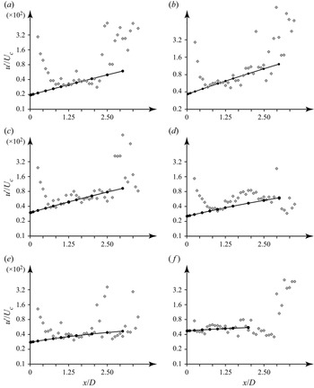
 $n=1$ is due to the Orr mechanism at shorter wavelengths, and due to the lift-up mechanism (called ‘shift-up’ because this mechanism at
 $n=1$ effectively shifts the jet) at long waves. Also, the rapid convergence of the optimal perturbation to a long-time asymptotic for the optimal growth derived by Ortiz & Chomaz (Reference Ortiz and Chomaz2011) was demonstrated. The work of Nastro, Fontane & Joly (Reference Nastro, Fontane and Joly2020) deals with a jet developing temporally due to the nonlinear evolution of a linear wave into a Kelvin–Helmholtz billow. This work explains earlier experimental observations by Liepmann & Gharib (Reference Liepmann and Gharib1992): during the development of axisymmetric Kelvin–Helmholtz billows, a generation of non-axisymmetric perturbations was observed in the braid region, which were further sucked into the upstream ring region. Originally, it was implied that this loss of axisymmetry is the result of a secondary instability of Kelvin–Helmholtz billows; however, a study by Nastro et al. (Reference Nastro, Fontane and Joly2020) suggests that the non-modal growth of non-axisymmetric perturbations to temporally developing axisymmetric Kelvin–Helmholtz billows could be responsible for that observation. To our knowledge, there are no more studies of non-modal growth in laminar jets and no attempts to investigate the non-modal route to transition experimentally.
Moreover, even modal stability theory has not been reliably verified in experiments with jets. The first tests with controlled perturbations of jet flows began more than 50 years ago by Vlasov & Ginevskii (Reference Vlasov and Ginevskii1967), who discovered that the intensity of turbulent mixing in a subsonic turbulent jet can be controlled by a weak acoustic excitation. It was observed that the excitations at low frequencies resulted in much better mixing than the excitations at frequencies that were an order higher. Extensive development of that work in regard to strong acoustic excitation of turbulent jets and their strong nonlinear evolution can be found in Ginevskii, Vlasov & Karavosov (Reference Ginevskii, Vlasov and Karavosov2004), Krivokorytov et al. (Reference Krivokorytov, Golub, Moralev and Volodin2014) and Kozlov et al. (Reference Kozlov, Grek and Litvinenko2016).
Later, based on experimental observations, Crow & Champagne (Reference Crow and Champagne1971) introduced the concept of the ‘jet preferred mode’, which is the evolution of a controlled perturbation with a Strouhal number  ${St} \approx 0.3$ that yields the fastest jet breakdown. Although the jet was turbulent, the amplitudes of the axisymmetric perturbations introduced in that experiment were not small, and the jet's response was essentially nonlinear so that the jet as a whole was twisted in shape, the observed wavelengths were in good agreement with calculations based on the eigenvalue problem for the Rayleigh equation, which was unexpected even for the authors of that study. Zaman & Hussain (Reference Zaman and Hussain1980) further studied controlled perturbations of a turbulent jet and suggested that there are actually two distinct preferred modes: ‘shear-layer’ and ‘jet-column’ modes. That is, they observed that the vortex pairing is most pronounced under controlled acoustic excitations at Strouhal number
 ${St} \approx 0.85$ and brings strong growth of the centre line fluctuation intensity, which was associated with the jet-column mode. However, Petersen & Samet (Reference Petersen and Samet1988) argued that these two types of the preferred mode are representations of the same mode at different distances from the orifice. They analysed Orr–Sommerfeld equations applied to an experimental jet profile (the same profile as in Crow & Champagne (Reference Crow and Champagne1971)) and proved that since there is no crucial difference between the preferred mode and shear layer instability, the preferred mode is actually the shear-layer mode that is most amplified at a distance of four jet diameters from the orifice.
The conclusion of Petersen & Samet (Reference Petersen and Samet1988) that the jet-column mode is the evolution of the shear-layer mode was later doubted by Burattini et al. (Reference Burattini, Antonia, Rajagopalan and Stephens2004), because they successfully excited the former independently from the latter. Specifically, they installed metal grids at the orifice to suppress the initial shear layer instability. The frequency of the jet preferred mode dominates in the spectrum only at  $x/D\ge 2$ when the grids are not used (in what follows, the
 $x$-axis is directed along the jet axis and
 $D$ is the jet diameter), and closer to the orifice when the grids are installed. The frequencies of the growing perturbations are well predicted by the inviscid linear stability theory, but the experimental growth rates are not in agreement with these predictions. The authors explain this discrepancy by the turbulence of the jet, given that the theory assumes laminar flow. The difference between the jet preferred mode and the shear-layer mode was also supported in experiments by Sadeghi & Pollard (Reference Sadeghi and Pollard2012). By installing a ring in the shear layer, they suppressed the Kelvin–Helmholtz instability and the subsequent vortex pairing, but the frequency of the jet preferred mode still exists in the fluctuation spectrum.
Arguments in support of the unity of the preferred mode were given by Garnaud et al. (Reference Garnaud, Lesshat, Schmid and Huerre2013). They studied mean turbulent jet flow (including its spreading downstream) and, by using resolvent analysis, considered two types of axisymmetric optimal forcing: one through the incoming velocity profile of the pipe feeding the jet, and the other through the volumetric momentum distribution in the feeding pipe. Both types of forcing yield a similar optimal response, with a maximum energy gain at  ${St}=0.46$, which was associated with the preferred mode of the turbulent jet. They showed that the optimal response follows the most unsteady local shear-layer mode near the feeding pipe, while farther downstream, when the shear-layer mode starts decaying, the optimal response switches to the least stable mode, which turns out to be the local jet-column mode. This transition theoretically explains the disagreement about the origin of the jet preferred mode and supports the conclusion of Petersen & Samet (Reference Petersen and Samet1988). The question of the nature of the preferred mode was readdressed in a recent experimental study by Mair et al. (Reference Mair, Bacic, Chakravarthy and Williams2020), but no definite conclusion was drawn by the authors.
Thus, currently, there is no consensus on the nature of the jet preferred mode, in both theoretical and experimental studies. As was argued by Mair et al. (Reference Mair, Bacic, Chakravarthy and Williams2020), this is partially a result of attempts to apply linear stability theory, which assumes laminar flow, to turbulent jet flows. Moreover, a numerical study by Boguslawski, Wawrzak & Tyliszczak (Reference Boguslawski, Wawrzak and Tyliszczak2019) clearly demonstrates that the turbulent jet's response to forced excitation depends not only on the jet's velocity profile, as linear stability theory predicts, but also on the combination of incoming turbulence intensity and excitation amplitude and frequency. In all cases, purely nonlinear mechanisms play a role in the development of perturbations in turbulent jets; in particular, although the theoretically predicted eigenmode was successfully excited for jet's with a thicker shear layer (which corresponds to the results of Crow & Champagne (Reference Crow and Champagne1971)), for the case of a thinner shear layer, the eigenmode had a higher frequency and was broken up by turbulent fluctuations so that the excitation did not affect the jet's dynamics.
A somewhat different direction in recent studies is the role of linear mechanisms in sustaining turbulence in developed turbulent jets. Although earlier it was assumed that the description of the generation and sustaining of turbulent fluctuations is possible only through a nonlinear analysis, including direct numerical simulation of the Navier–Stokes equations, starting from the fundamental work by Trefethen et al. (Reference Trefethen, Trefethen, Reddy and Driscoll1993), many studies shifted to linear but non-modal mechanisms of perturbation growth. As was discussed in detail by Trefethen et al. (Reference Trefethen, Trefethen, Reddy and Driscoll1993), there are two, in many senses equivalent, formulations of the non-modal growth problem. The first is the problem of optimal perturbation, i.e. finding optimal initial conditions that provide the largest energy growth at a given time (temporal problem) or a given axial coordinate (spatial problem). The second is the problem of optimal forcing, i.e. optimal harmonic excitation that provides the largest energy (or other appropriate norm) of the flow response, which is also known as resolvent analysis. As turbulent jets are approximately linearly spreading with the axial coordinate, the assumption of plane-parallel base flow is doubtful, which is why recent studies consider fully two-dimensional axisymmetric base flow (with non-zero axial and radial velocity distributions that depend on both axial and radial coordinates) and perform global linear analysis. The work of Garnaud et al. (Reference Garnaud, Lesshat, Schmid and Huerre2013) attempted to resolve the question of the nature of the jet preferred mode through a linear resolvent analysis. A natural question is, to what extent does the linear analysis of mean turbulent flow represent the actual dynamics of unsteady turbulent flow? To address this question, Semeraro et al. (Reference Semeraro, Lesshafft, Jaunet and Jordan2016) considered a somewhat similar type of global linear axisymmetric resolvent analysis of mean turbulent jet flow (the only difference with Garnaud et al. (Reference Garnaud, Lesshat, Schmid and Huerre2013) is that the jet was compressible with  $M=0.9$) and compared the results with careful experimental measurements and large-eddy simulation (LES). It was demonstrated that although experiment and LES calculations were in good agreement, the prediction of the linear resolvent analysis was acceptable only for Strouhal numbers
 $0.3<{St}<0.8$ and only near the nozzle. The authors noted the similarity of the limitation of the linear analysis of fully two-dimensional base flow with other problem formulations (see references in Semeraro et al. (Reference Semeraro, Lesshafft, Jaunet and Jordan2016) for details).
A promising development in the resolvent analysis of turbulent jets was proposed by Pickering et al. (Reference Pickering, Rigas, Nogueira, Cavalieri, Schmidt and Colonius2020, Reference Pickering, Rigas, Schmidt, Sipp and Colonius2021). They included the spatial variation in mean turbulent viscosity in the linearized Navier–Stokes equations and showed that the correlation with the LES data becomes better. They considered not only axisymmetric perturbations but also perturbations with azimuthal wavenumbers 1–5. By analysing the qualitative structure of forcing and response velocity fields at different Strouhal numbers and azimuthal wavenumbers, they revealed which of the three linear growth mechanisms, modal Kelvin–Helmholtz and non-modal the Orr and lift-up mechanisms, are responsible for the energy growth. For compressible jets with  $M=0.4$, 0.9 and 1.5, the results turned out to be similar: Orr mechanism dominates in axisymmetric quasi-steady perturbations (
 $n=0$,
 ${St}\approx 0$); the lift-up mechanism dominates in non-axisymmetric quasi-steady perturbations (
 $n>0$,
 ${St}\approx 0$); the Kelvin–Helmholtz mechanism dominates at
 $n=0, 1$ and
 $0.5<{St}<1.0$; other ranges of the azimuthal wavenumbers and Strouhal numbers give a much weaker response to harmonic forcing. These results suggest that linear analysis, also encompassing variable turbulent viscosity, can indeed predict the dominant energetic structures in a turbulent jet and that linear mechanisms are in many ways responsible for the generation of large-scale turbulent fluctuations.
Velocity fluctuations in an unexcited turbulent jet with  $Re \sim 10^{5}$ were thoroughly measured by Jung, Gamard & George (Reference Jung, Gamard and George2004) using an array of 138 hot-wire probes. They applied proper orthogonal decomposition (POD) to obtain experimentally the most energetic modes and then to reconstruct the instantaneous fluctuating velocity field to find the dominant structures in the turbulent jet. It appeared that more than
 $60\,\%$ of the resolved streamwise turbulent energy is contained in the first POD mode. From the jet's origin to
 $x/D\approx 4$, the axisymmetric POD mode shows the fastest growth and afterwards stabilizes, giving a path to the rapid growth of higher modes. The downstream behaviour of the eigenmodes corresponds qualitatively to the inviscid linear stability theory. Batchelor & Gill (Reference Batchelor and Gill1962) showed that the axisymmetric mode grows strongest for the initial ‘top-hat’ jet profile but starts decaying during the downstream evolution of the jet so that the only mode with azimuthal wavenumber
 $n=1$ stays stable for the ‘far-downstream’ profile. A good correlation between the wavelength of the most energetic POD modes in fully developed turbulent jets and linear stability theory was also noted by Mullyadzhanov et al. (Reference Mullyadzhanov, Sandberg, Abdurakipov, George and Hanjalić2018) in their analysis of direct numerical simulation.
An interesting study by Lemanov, Lukashov & Sharov (Reference Lemanov, Lukashov and Sharov2020) demonstrated a new mechanism of transition to turbulence. A jet flows out of a pipe with Reynolds numbers  $Re=1900 - 3500$, at which the pipe flow was intermittent: mostly laminar with localized turbulent puffs. The jet flow, consequently, was also intermittent starting from the orifice, and the transition to turbulence included the evolution of turbulent puffs in the jet.
Returning to laminar jets and their transition to turbulence, there is no doubt that the modal growth of perturbations plays a primary role, which yields the formation of Kelvin–Helmholtz billows, visible in all experimental and numerical studies, and their further breakdown. Moreover, in contrast to wall-bounded flows, in which the modal instability is weaker than the inviscid instability of jet flows, the initial non-modal growth does not yield a local maximum of the optimal energy gain curve but just increases the amplitude of the fastest growing eigenmode (Jiménez-González et al. Reference Jiménez-González, Brancher and Martínez-Bazán2015), which then follows the long-time asymptotic of Ortiz & Chomaz (Reference Ortiz and Chomaz2011). It is also worth noting that in laminar jets, a local approach is more adequate than in turbulent jets, because the spatial development of steady laminar flows is much slower than that of turbulent flows. Note that Boronin et al. (Reference Boronin, Healey and Sazhin2013) and Jiménez-González et al. (Reference Jiménez-González, Brancher and Martínez-Bazán2015), who first studied non-modal linear growth in laminar jets, considered plane-parallel (i.e. non-developing downstream) base flow.
To our knowledge, the only attempts to experimentally correlate small perturbations of the jet flow in its laminar portion with linear stability theory were made by Cohen & Wygnanski (Reference Cohen and Wygnanski1987) and Petersen & Samet (Reference Petersen and Samet1988). Cohen & Wygnanski (Reference Cohen and Wygnanski1987) experimentally studied the evolution of axisymmetric and helical modes (excited acoustically) in axisymmetric jet at a Reynolds number of  $24\,000$. Phase-locked measurements have been made using eight thermoanemometers at downstream distances
 $x/D\le 0.7$. The theoretically and experimentally obtained amplitude and phase distributions in the forced jet were in good agreement, although the spatial growth rate of the excited perturbation was
 $2 - 3$ times lower than predicted theoretically. The wavelengths of the perturbations were not measured, because they were larger than the distance at which the transition to turbulence occurred. The same facility was used for the comparison of experimental and theoretical results for the jet's stability characteristics by Petersen & Samet (Reference Petersen and Samet1988). The velocity regime at which the measurements were made was higher:
 $Re = 56\,000$; and the downstream distances of the measurements were larger, up to
 $x/D=5$. Although the transition to turbulence occurred near the orifice,
 $0.5< x/D<1$, the radial distributions of the amplitude and phase of the axial velocity perturbations, as well as the phase speed measured at different streamwise locations, were in good agreement with the predictions of linear stability theory, obtained through the Orr–Sommerfield equation in the laminar, transitional and fully turbulent regions of the jet.
It must again be noted that most of the experiments reviewed above, as well as many others in which the jet was excited, dealt with turbulent jets. Clearly, linear stability theory provides important mechanisms for sustaining large-scale turbulent fluctuations, but the quantitative correlations with experiments are good only in terms of specific quantities under specific flow conditions and fail under other conditions (Semeraro et al. Reference Semeraro, Lesshafft, Jaunet and Jordan2016; Boguslawski et al. Reference Boguslawski, Wawrzak and Tyliszczak2019). This inconsistency is natural, because turbulence inevitably includes nonlinear effects, whose precise role is still not fully clear. A disagreement between the theoretical and experimental growth rate (Cohen & Wygnanski Reference Cohen and Wygnanski1987) in a laminar jet also keeps open the question of the role of nonlinearity in the initial stage of perturbation evolution.
The only experiments by Cohen & Wygnanski (Reference Cohen and Wygnanski1987) and Petersen & Samet (Reference Petersen and Samet1988) on controlled excitation of a laminar portion of the jet suffer from a very short laminar region (shorter than one diameter), which did not allow measuring wavelengths and spatial growth rates within the laminar region. The main obstacle to obtaining a long laminar portion of the jet is the extremely low critical Reynolds number of jet flows, ranging from  $14$ to
 $44$ (Morris Reference Morris1976; Shtern & Hussain Reference Shtern and Hussain2003; Mullyadzhanov & Yavorsky Reference Mullyadzhanov and Yavorsky2018), depending on the problem formulation and assumptions and, consequently, jet breakdown within one or two diameters from the orifice at large Reynolds numbers. Given that, on the one hand, experiments on perturbation growth should be conducted with sufficiently thick jets to be able to perform detailed experimental measurements of perturbations and that, on the other hand, the distance to transition should be sufficiently long to capture at least several wavelengths, it is extremely difficult to organize such laminar jet flow.
Recently, our group proposed a new technique for the generation of laminar jets (Zayko et al. Reference Zayko, Teplovodskii, Chicherina, Vedeneev and Reshmin2018). The experimental facility provides a submerged air jet of diameter  $D=0.12$ m with Reynolds numbers of up to
 $10 \, 000$ (below, unless otherwise specified, the Reynolds number is based on the jet diameter
 $D$ and the velocity averaged over the cross-section) and a length of the laminar region of up to five jet diameters. Such parameters provide excellent conditions for the experimental analysis of small controlled perturbations in laminar jet. Moreover, the jet profile obtained in our experiments has three inflection points, yielding two different axisymmetric instability modes with a similar frequency range but different wavelengths and radial distributions of fluctuations (unlike classical ‘top-hat’, parabolic or ‘far-downstream’ profiles with one inflection point and at most one mode of instability for each azimuthal wave number). Separate excitation and experimental analysis of these two modes is a more sophisticated benchmark for linear stability theory than classical jet profiles. This is the goal of the present study.
The paper is organized as follows. Section 2 is devoted to the theoretical analysis of jet instability. Section 3 describes the experimental facility and the study of controlled perturbations. Section 4 is devoted to the comparison of theoretical predictions with experimental data and § 5 summarizes the results and concludes the paper.
2. Theoretical study of perturbation growth in a submerged jet
In this section, we theoretically study perturbation growth in an experimentally obtained axisymmetric jet. Zayko et al. (Reference Zayko, Teplovodskii, Chicherina, Vedeneev and Reshmin2018) discussed in detail the forming device and the jet properties, so we only briefly describe them here.
2.1. Jet-forming device
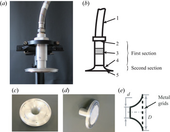
The air jet is formed by a device that consists of two principal sections (figure 1a,b). The first section reduces the turbulent fluctuations of the incoming flow and consists of a tube of length  $0.14$ m and inner diameter
 $0.04$ m. At the inlet of the tube, a perforated plate with holes of diameter
 $0.6$ mm and a holes-to-plate area ratio of
 $0.8$ is installed. A bushing with two metal grids is located downstream the plate: the first grid at a distance of
 $0.3$ m; the second at
 $0.8$ m from the plate. The wire diameter of the first grid is
 $0.05 \pm 0.004$ mm and that of the second grid
 $0.03 \pm 0.004$ mm; their free area ratios are
 $34.4\,\%$ and
 $32.7\,\%$, respectively. The second section is a short round diffuser with length
 $0.04$ m, inlet diameter
 $d = 0.04$ m and outlet diameter
 $D = 0.12$ m (figure 1c,d,e). Two metal grids are stretched at the diffuser outlet to prevent flow separation from the wall (figure 1d,e).
Photograph (a) and sketch (b) of the forming device: pipeline (1), perforated plate (2) and bushing with two metal grids (3), and diffuser (4) with metal grids (5). Photograph of the diffuser without (c) and with (d) metal grids and its sketch (e).

In this study, we consider a flow regime with a velocity at the jet axis of  $U_{c} = 1.5\,\mathrm {m}\,\mathrm {s}^{-1}$, which corresponds to Reynolds number
 $Re=5400$ (the jet diameter is
 $D=0.12$ m, and the velocity
 $U_{av}$ averaged over the jet's cross-section is
 $0.66\,\textrm {m}\,\textrm {s}^{-1}$). As shown by Zayko et al. (Reference Zayko, Teplovodskii, Chicherina, Vedeneev and Reshmin2018), at this regime the jet is laminar up to a distance
 $x/D=5$ from the diffuser outlet (below we will call this the ‘orifice’ for brevity).
2.2. Base velocity profiles at different spatial locations
To get smooth axial velocity profiles  $U(r)$, where
 $r$ is the radial coordinate, we performed laminar-flow calculations of the jet flow. To make sure that the calculations represent the real jet, the obtained profiles of axial velocity were compared with experimental profiles measured by a thermoanemometer at different axial locations. After that, the calculated profiles were approximated by analytical functions, which were finally used in the stability analysis.
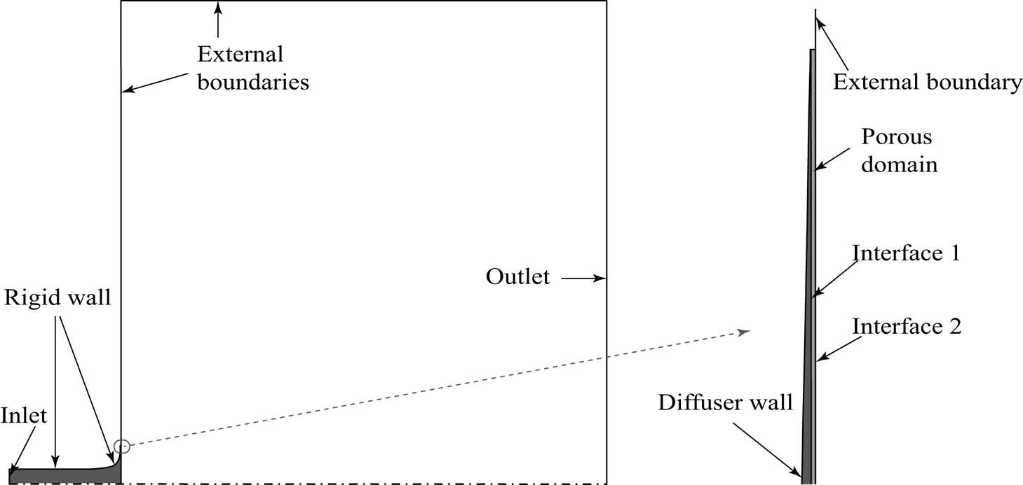
As the jet is laminar, we conducted steady-state laminar calculations to obtain velocity profiles at different distances from the orifice. The Navier–Stokes equations were solved by the control volume method implemented in the Ansys CFX solver. Due to the axisymmetry of the forming device and the flow, the computational region was chosen to be the  $5^{\circ }$ sector, with symmetry conditions at the sector's side planes (figure 2). The tube and the diffuser (deep grey in figure 2) and the ambient area (white in figure 2) are incompressible fluid domains. The porous domain (light grey in figure 2) models the metal grids at the diffuser outlet. To describe the momentum loss at the grids, permeability and resistance loss coefficients of the porous medium were specified according to experimentally measured pressure drops at the grids (Zayko et al. Reference Zayko, Teplovodskii, Chicherina, Vedeneev and Reshmin2018). The outlet section and horizontal external boundary were located at distances
 $5D$ and
 $5.5D$ from the porous domain and the axis, respectively. We have also checked a longer domain in streamwise direction (
 $10D$) to make sure that the velocity distribution for
 $x/D\le 3$ is converged.
Computational region consisting of the tube and diffuser (deep grey domain), the porous domain (light grey domain) and the ambient fluid region (white domain).

A normal velocity of  $5.9\,\textrm {m}\,\textrm {s}^{-1}$ was specified at the inlet (which corresponds to velocity
 $1.5\,\textrm {m}\,\textrm {s}^{-1}$ at the jet axis), no-slip condition at the diffuser wall, and a pressure of
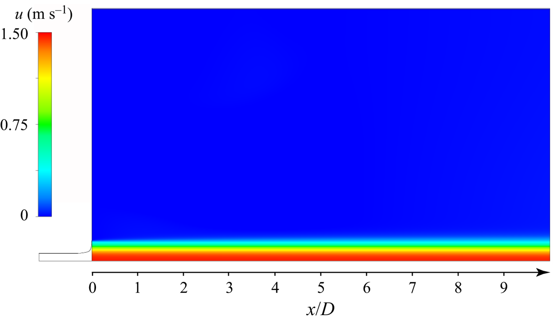
 $10^{5}$ Pa at the external boundaries and outlet; additionally, a zero gradient of the flow direction was specified at the external boundaries. Details of the computational mesh and convergence study can be found in Zayko et al. (Reference Zayko, Teplovodskii, Chicherina, Vedeneev and Reshmin2018). Figure 3 shows the calculated laminar jet flow, which turns out to be just slightly developing at the distance
 $x/D\le 10$.
Distribution of axial velocity in the developing jet (streamwise domain length is  $10D$).

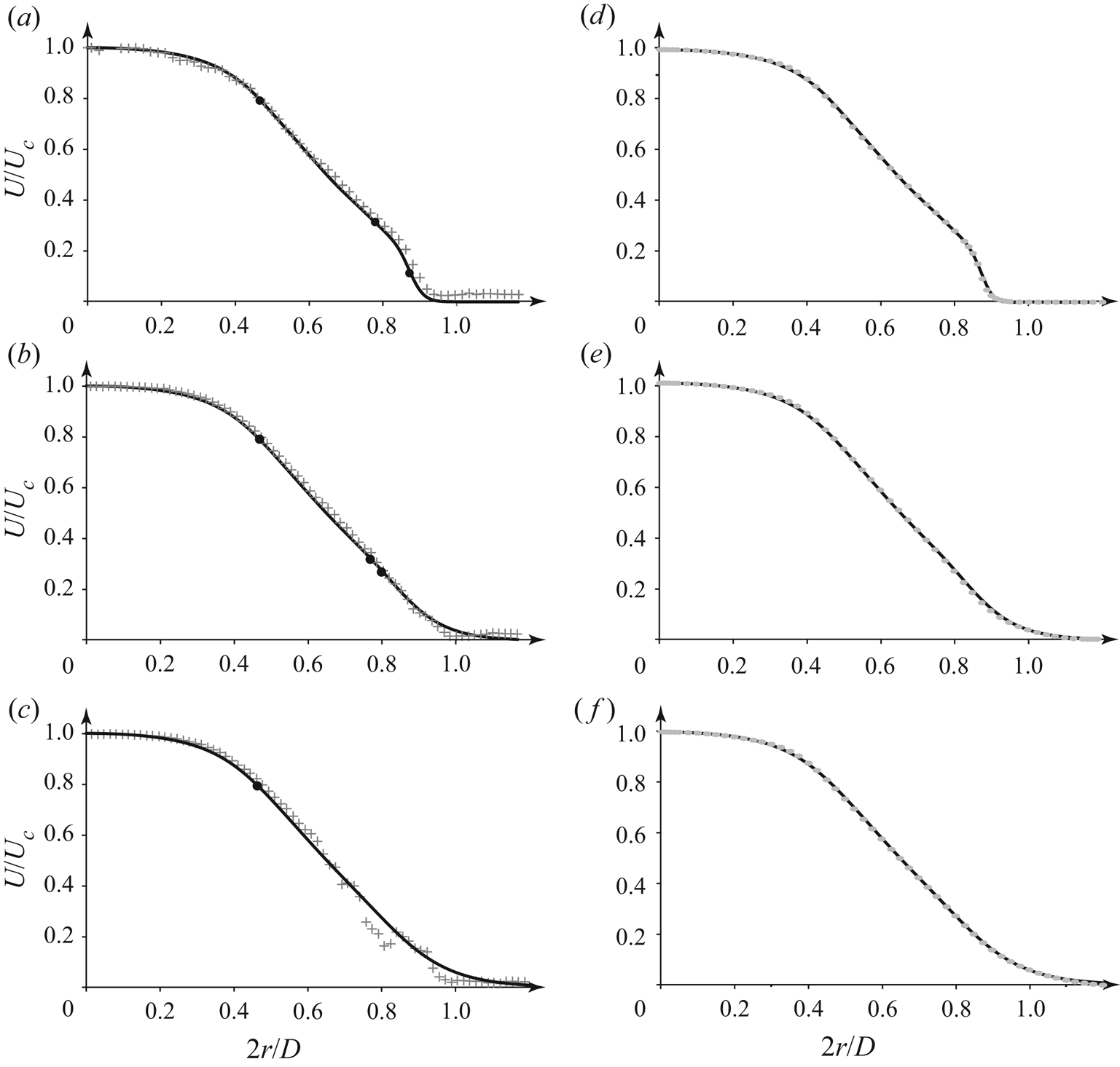
The comparison of numerical and experimental profiles is shown in figure 4(a–c). It is seen that the correlation is good at distances  $x/D\le 1.5$ (figure 4a,b); however, farther downstream at
 $x/D=3$, some discrepancy appears at the outer jet region (figure 4c) due to an apparent irregularity in the experimental velocity profile. We explain this irregularity by growing velocity fluctuations, possibly nonlinear, which, however, do not break up the laminarity of the flow, as was confirmed by visualization (see § 3.2 below). Nevertheless, the deviation between the experiment and the calculation is not large even at
 $x/D=3$ (the largest distance that will be analysed in this study) so that we consider the calculated profiles acceptable.
Comparison of experimental (crosses) and numerical (lines) velocity profiles (a–c). Comparison of numerical (lines) and analytical (markers) velocity profiles (d–f). Distance  $x/D = 0.01$ (a,d),
 $1.5$ (b,e) and
 $3$ (c,f) from the orifice; the circles denote generalized inflection points for azimuthal wavenumber
 $n=0$.

An important characteristic of the velocity profile in the context of linear stability analysis is generalized inflection points, i.e. points at which
 \begin{equation} \frac{\textrm{d}}{\textrm{d}r}\left( \frac{rU'}{n^2 + \alpha^2r^2} \right) = 0, \end{equation}
where the prime denotes the derivative with respect to  $r$;
 $\alpha \in \mathbb {C}$ and
 $n\in \mathbb {Z}$ are axial and azimuthal wavenumbers, respectively. Near the orifice, there are three generalized inflection points: two of them are located near the jet boundary, and the third is closer to the jet axis (figure 4a). The two generalized inflection points near the jet boundary get closer to each other when moving downstream (figure 4b), and they merge at a distance
 $x/D \approx 1.8$. Consequently, only one generalized inflection point remains in the profiles at distances larger than
 $1.8D$ (figure 4c). Note that
 $U_{c}$ does not change significantly with increasing distance from the orifice: for instance, the difference between
 $U_{c}$ at
 $x/D = 0.5$ and
 $x/D = 1.75$ is approximately
 $1\,\%$.
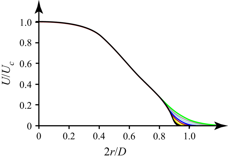
In the theoretical analysis, it is convenient to approximate the calculated base velocity (defined on a finite-volume grid) by an analytical function, because it readily provides the first and second derivatives, avoiding errors of differentiation of the grid-defined function. The results of the approximation at different distances from the orifice are shown in figure 4(d–f), and an excellent correlation is clear. The set of resulting base profiles is summarized in figure 5. It is seen that the evolution of the velocity profiles downstream consists of a slight viscous spreading near the jet boundary.
Analytical axial velocity profiles at distances from the orifice of  $x/D=0.01$,
 $0.04$ (black),
 $0.1$ (yellow),
 $0.25$ (red),
 $0.5$ (deep blue),
 $1$ (light blue),
 $2$ (grey) and
 $3$ (green).

2.3. Formulation of the stability problem
Because of sufficiently large Reynolds number, the instability analysis was based on inviscid linear stability theory. To obtain a dimensionless problem formulation, the velocities are non-dimensionalized by  $U_{c}$, and the distances by
 $D/2$. The Euler equations linearized around the steady-laminar unidirectional jet with a given velocity profile yield the Rayleigh equation for a radial velocity perturbation,
 \begin{align} (U(r) - c)\frac{\textrm{d}}{\textrm{d}r}\left( \frac{r}{n^{2}+\alpha^{2}r^{2}} \frac{\textrm{d}(rG(r))}{\textrm{d}r} \right) - ( U(r) - c )G(r) - rG(r)\frac{\textrm{d}}{\textrm{d}r}\left( \frac{rU^{'}(r)}{n^{2}+\alpha^{2}r^{2}} \right) = 0, \end{align}
where  $G(r)$ is the amplitude of the radial velocity fluctuation
 $u_{r}=iG(r)\exp (\textrm {i}(\alpha x + n\phi - \omega t))$,
 $\omega \in \mathbb {R}$ is the frequency and
 $c = \omega / \alpha$ is the phase speed. A similar equation for a plane-parallel flow was first obtained by Rayleigh (Reference Rayleigh1892), and its form (2.2) for the axisymmetric flow was derived by Batchelor & Gill (Reference Batchelor and Gill1962). The dimensionless frequency
 $\omega$ is related to the physical dimensional frequency
 $\varOmega$ as
 \begin{equation} \omega = \frac{2{\rm \pi} \varOmega}{U_{c}} \frac{D}{2}. \end{equation}
The dimensionless wavenumber  $\alpha$ defines the dimensional growth rate
 $\delta$ and wavelength
 $\lambda$ through the relations
 \begin{equation} \delta ={-}\mathrm{Im}\, \alpha\left(\frac{D}{2}\right)^{{-}1} \quad \mathrm{and} \quad \lambda = \frac{2{\rm \pi}}{\mathrm{Re}\, \alpha} \frac{D}{2}, \end{equation}
respectively.
The function  $G(r)$ should satisfy two boundary conditions. The first condition at
 $r=0$ is the following (see Batchelor & Gill (Reference Batchelor and Gill1962) for details):
 \begin{equation} \left. \begin{array}{ll@{}} G(0) = 0 & \mathrm{for} \ n=0, \\ G'(0) = 0 & \mathrm{for} \ n=1, \\ G(r) \sim r^{n-1}, \; r \to 0 & \mathrm{for} \ n>1. \end{array} \right\} \end{equation}
The condition at  $r=1$ is the radiation condition transferred from infinity,
 \begin{equation} \frac{G'(r)}{G(r)} = \frac{\textrm{K}''_n (\alpha r)}{\textrm{K}'_n(\alpha r)} \quad \mathrm{for} \ r=1, \end{equation}
where  $\textrm {K}_n$ is the modified Bessel function of the second kind.
The boundary-value problem (2.2), (2.5), (2.6) defines an eigenvalue problem to find  $\alpha (\omega, n) \in \mathbb {C}$ for each
 $\omega \in \mathbb {R}$,
 $n \in \mathbb {Z}$. Condition (2.5) selects one of two linearly independent solutions of the Rayleigh equation. Integrating this solution by the Runge–Kutta method from
 $r=0$ to
 $r=1$, we obtain the function
 $g(\alpha, n, \omega ) = G'(1)\textrm {K}'_n (\alpha ) - G(1)\textrm {K}''_n(\alpha )$. To satisfy condition (2.6), the root
 $\alpha (\omega, n)$ of the equation
 $g(\alpha, n, \omega ) = 0$ is found by the secant method.
For the stability analysis, we used velocity profiles at different distances from the orifice (figure 5). At a given distance, a weak dependence of the velocity on the axial coordinate was neglected when integrating (2.2), thus providing the parametric dependence  $\alpha (\omega, n, x)$ on
 $x$ through the base velocity profile slowly varying with
 $x$. This dependence on
 $x$ necessarily requires a small non-zero radial velocity component of the base flow, which was also neglected. Such a local approach is typical for base flows that are slowly varying in space, to which belongs the laminar jet at large Reynolds numbers. To restore the global spatial growth of the perturbation from the local linear stability analysis, local amplifications
 $\exp (-\mathrm {Im} \alpha (\omega, n, x) \Delta x)$ in every small axial segment
 $\Delta x$ can be multiplied to give the global amplification
 $\exp (-\int \mathrm {Im} \alpha (\omega, n, x)\,{\textrm {d}\kern0.7pt x})$. From this expression, the so-called
 $N$-factor can be extracted for a fixed azimuthal wavenumber
 $n=n_0$ as
 \begin{equation} N(x)=\max_{\omega}\int_{x_0}^x (-\mathrm{Im} \alpha(\omega, n_0, x)) \,{\textrm{d}x}, \end{equation}
which characterizes the global perturbation growth at a given  $x$ as
 $\textrm {e}^{N(x)}$.
2.4. Results of the linear stability analysis
First, consider the results for an axisymmetric perturbation with  $n=0$. The aim of the study is to compare the predictions of the linear theory with experiments, and an axisymmetric perturbation is the most convenient one to experimentally introduce into the jet.
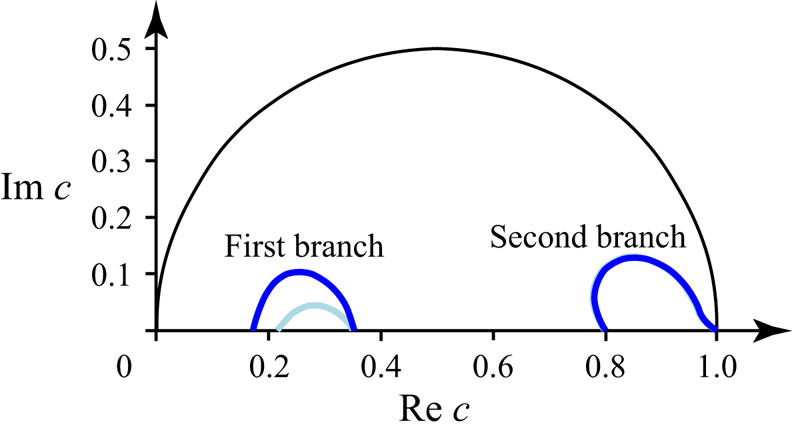
We found two branches of growing perturbations at  $n=0$. The first branch is generated by two generalized inflection points near the jet boundary, because the curve
 $c(\omega ) = \omega /\alpha (\omega )$,
 $\omega \in \mathbb {R}$, connects two neutral phase speeds equal to the velocities at the corresponding inflection points (figure 6). The second branch is generated by the generalized inflection point that is the closest to the jet axis: the corresponding
 $c(\omega )$ curve connects the phase speed equal to the velocity at this point with
 $c=1$ (figure 6). The modes of the first branch disappear at distances
 $x > 1.8D$ due to the disappearance of two outer generalized inflection points.
Branches of growing perturbations for velocity profiles at  $x/D=0.5$ (deep blue) and
 $x/D=1$ (light blue) in the complex half-plane,
 $c$. The curves for the second branch coincide.

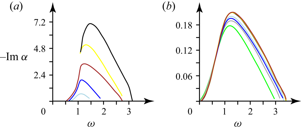
The spatial growth rates  $-\mathrm {Im} \alpha$ of the first branch of growing perturbations are greater than those of the second branch (figure 7). The frequency range of growing perturbations is
 $\omega = 0$–3.3 for both branches, except for the profiles that are extremely close to the orifice (see figure 7). The corresponding range of Strouhal numbers
 ${St} = \varOmega D/U_{c}$ is
 ${St} = 0$–1.06. The frequencies of the most growing perturbations are similar for both branches and lie in the range 1–1.76 (
 ${St} = 0.33$–0.57).
The theoretical dimensionless spatial growth rate  $-\mathrm {Im} \alpha$ versus the dimensionless excitation frequency
 $\omega$ at different distances from the orifice
 $x/D \ge 0.04$ (the colour coding corresponds to that in figure 5) for the first (a) and second (b) branches of growing perturbations.

In the case of the second branch, the range of the frequencies of the most growing perturbations, as well as the value of the growth rate, does not significantly differ for the profiles at different distances from the orifice (figure 7b). For the first branch, the perturbations grow faster, and the growth rates significantly depend on the distance from the orifice, but the frequencies corresponding to the maximum growth do not leave the range 1–1.76.
It is worth noting that in classical jet flows with one inflection point, their instability mode corresponds to the second mode of the present jet, which is clearly seen when the two outer inflection points merge and disappear, after which the first mode is decaying so that only the second mode keeps growing.
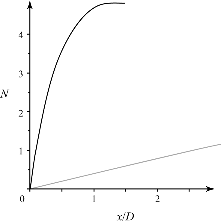
Although the first mode is growing in a limited range of  $x/D$ (up to the collapse of the two outer generalized inflection points), its growth in the initial jet region is stronger than that of the second mode, as can be estimated by the
 $N$-factor (2.7) shown in figure 8. Hence, if both modes are excited with comparable and sufficiently large amplitudes, the transition to turbulence will be triggered by the first mode. However, if the initial amplitudes are small enough, and the first mode starts decaying before the manifestation of nonlinear effects, then the transition will be triggered farther downstream by the second mode.
The  $N$-factors calculated for the first (black) and second (grey) modes.

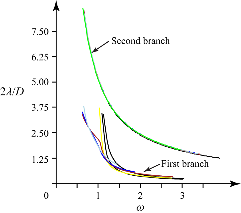
Figure 9 shows that the wavelengths of the first branch are shorter than those of the second branch, which provides a clear way to experimentally distinguish the observed perturbation modes.
The theoretical dimensionless wavelengths  $2\lambda /D$ versus the dimensionless excitation frequency
 $\omega$ (the colour coding corresponds to that in figure 5).

The calculations show that for  $n>0$, there are at most two branches of growing perturbations. For the second branch, growing perturbations exist only for
 $n=0$,
 $1$; for
 $n\ge 2$ these modes are decaying. The perturbations of the first branch have the largest maximal growth rates at
 $n=0$ for the profiles at distances
 $x/D = 0.01$,
 $0.04$,
 $0.1$,
 $0.25$,
 $0.5$, and at
 $n=1$ for
 $x/D = 1$,
 $1.5$. These maxima decrease with increasing
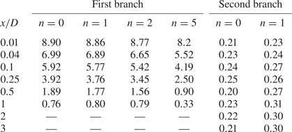
 $n$ (table 1). We have observed similar behaviour in the temporal stability analysis of the velocity profiles near the orifice at different flow regimes (Zayko et al. Reference Zayko, Teplovodskii, Chicherina, Vedeneev and Reshmin2018).
Maximum dimensionless growth rates  $-\mathrm {Im} \alpha$ for different azimuthal wave numbers
 $n$ at different distances from the orifice.

3. Experimental study of perturbation growth in a submerged jet
In this section, we describe an experimental study of controlled perturbations in a submerged jet. Two series of experiments were conducted: first, we investigated perturbations of the first branch (generated by inflection points near the jet boundary); second, perturbations of the second branch were considered. Below, we use dimensional physical frequencies  $\varOmega$ (Hz) and wavelengths
 $\lambda$ (m) to compare the experimental results with the theoretical predictions.
3.1. Experimental apparatus for the generation of controlled perturbations
Axisymmetric perturbations are the fastest growing perturbations of the considered jet and the most convenient to introduce them into the flow. The theoretically predicted physical frequencies  $\varOmega$ of the most growing perturbations are too low (
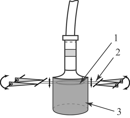
 $\approx 0 - 13$ Hz) for using acoustic excitation so that we decided to introduce the perturbations mechanically. Two thin metal strings were pulled on two drivers at a distance
 $x = 19$ mm (
 $\approx 0.16D$,
 $D=0.12$ m) from the orifice, and a ring made of a wire was fixed on the strings coaxially with the jet (figure 10). The string thickness is
 $0.2$ mm (
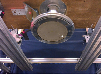
 $\approx 0.0017D$), and the strings do not significantly affect the jet both at rest and during oscillations along the jet axis. The oscillations are governed by the drivers, and they have specified amplitudes and frequencies. In each series of experiments, one of the two rings was used. The first ring had a diameter of
 $102.4$ mm (
 $0.85D$), and the second ring had a diameter of
 $56.9$ mm (
 $0.47D$) (figures 11 and 12). We chose these specific diameters to locate the first (large) ring between the two outer generalized inflection points, and the second (small) ring approximately under the internal generalized inflection point. The large and small rings had to amplify the disturbances of the first and second branches of growing perturbations, respectively. The thicknesses of the large and small rings’ wires are
 $0.8$ mm and
 $0.4$ mm (
 $\approx 0.0066D$ and
 $0.0033D$), respectively. At the considered velocity regime, the Reynolds numbers of the flows around their cylindrical cross-sections are
 $42.4$ and
 $35.5$, and both are below the critical value of
 $47$ (Roshko Reference Roshko1954) so that von Kármán vortex streets are not formed downstream the rings.
Sketch of ring (1) on the strings (2) in the jet (3). The ring is located coaxially with the jet. The strings are oscillated by the driver in the axial direction.

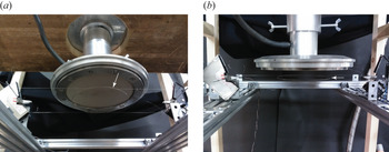
The large ring (indicated by the arrow) that introduces controlled disturbances of the first branch of growing perturbations.

The small ring (indicated by the arrow) that introduces controlled disturbances of the second branch of growing perturbations.

3.2. Visualization
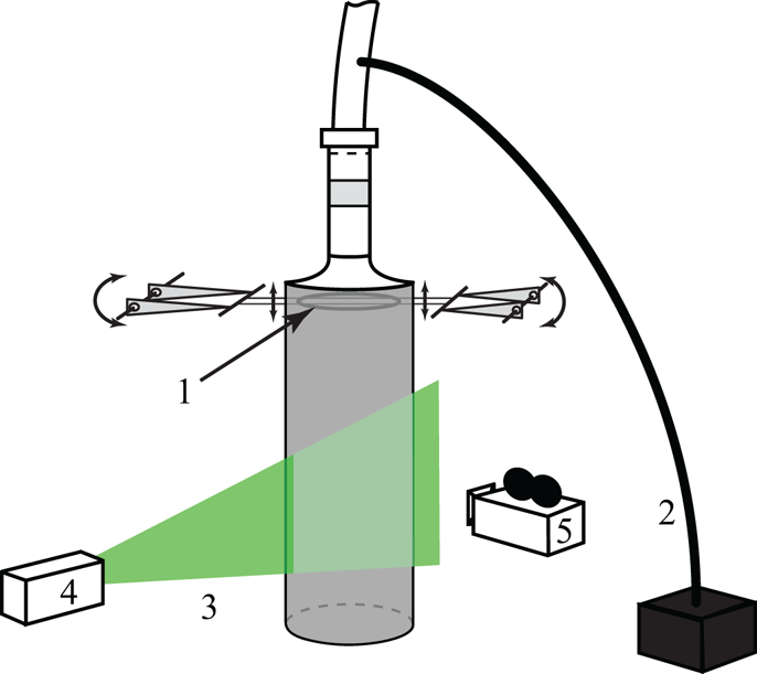
We put small reflective glycerin particles into the jet to visualize the flow. A plane section, passing through the jet axis, is lighted by a laser sheet, which is generated by a Beamtech Vlite-Hi-100 laser. The jet is filmed by a Canon EOS 600D camera (figure 13).
Oscillating ring (1), tube for putting the reflective glycerine particles into the flow (2), laser light sheet (3), laser (4) and video camera (5).

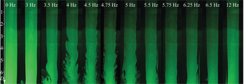
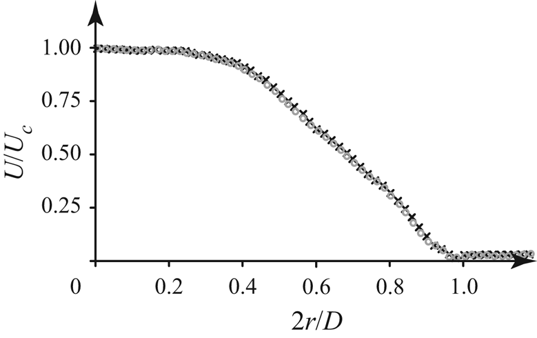
We performed visualization experiments with the first ring. First, we checked that the resting ring does not violate the laminar character of the jet (see the first photograph in figure 14) and does not significantly change the velocity profile (figure 15). The first series of experiments was conducted at different oscillation frequencies with a constant ring displacement amplitude, and the subsequent series were conducted at a constant amplitude of the oscillations’ velocities. First, at a frequency  $\varOmega =4.75$ Hz (
 ${St} = 0.38$), the amplitude of the ring oscillations was chosen to be
 $0.9$ mm. At this amplitude, the influence of the oscillations on the jet is noticeable, but it is not so large that the jet breaks down close to the orifice. Then, in the first visualization series, the displacement amplitude was approximately equal to this value for various oscillation frequencies. This displacement amplitude at
 $4.75$ Hz corresponds to the amplitude of an oscillation velocity of
 $0.027\,\textrm {m}\,\textrm {s}^{-1}$. In the subsequent series of visualization experiments, we kept this value at
 $0.027 \pm 0.003\,\textrm {m}\,\textrm {s}^{-1}$ for different frequencies of the ring oscillations.
Photographs of the jet under the oscillations of the first (large) ring with different frequencies at a constant amplitude of the velocity of the ring's oscillations. The axial distance is measured from the ring's location.

Velocity profiles at a distance  $x/D = 0.54$ without the large ring (black crosses), and with the large ring resting (grey circles).

The filming of the jet was conducted at frequencies of the ring oscillations of  $0 - 12$ Hz with a step of
 $0.25$ Hz – figure 14 shows several samples.
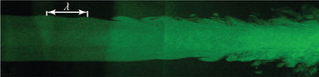
In the region of linear growth (before the start of the formation of Kelvin–Helmholtz billows), we measured the lengths of sinusoidal waves over the jet boundary using movie snapshots. Specifically, we measured the distance between two successive humps in a computer image, as shown in figure 16. This value was then scaled to millimetres with a calibration picture of a ruler located at the same distance from the camera as the laser sheet. This process has two sources of inaccuracy. First, the resolution of the computer image was 184 pixels per 100 mm; hence, the inaccuracy caused by a one-pixel error yields a physical error of less than 0.5 mm. Second, the human eye leads to inaccuracy in the selection of the highest points on the humps. We estimated that this inaccuracy does not exceed  ${\pm }3$ mm at each hump; given that there are two humps, we obtain a total inaccuracy of the measured wavelength of not more than
 ${\pm }6$ mm. Measuring the distance between two humps that are remote from each other makes the inaccuracy even lower than this value. The obtained wavelengths were compared with the theoretically calculated values.
Wavelength of the disturbance at the jet boundary under the first ring's oscillations with a frequency of  $4.5$ Hz.

For the second branch, we failed to obtain corresponding wavelengths from the visualization during the small ring's oscillations: at the same amplitude as for the large ring, there was no visually noticeable perturbation of the jet boundary; i.e. the second mode was localized inside the jet.
3.3. Measurements of velocity fluctuations and correlation analysis
To find the wavelengths of the second branch of growing perturbations, we used the correlation between the velocity fluctuations and the location of the oscillating ring. The same method was employed to double-check the wavelengths of the first branch (obtained from the visualization). The velocity fluctuations were also used directly for the analysis of their spatial distribution and growth rate.
A DISA 56C01 CTA thermoanemometer was used for the velocity measurements. The signal was transferred to an analogue-to-digital converter connected to a personal computer. The velocity was measured by small-sized Dantec Dynamics 55P11 probes. The probe has a wire sensor mounted on two straight needle-shaped prongs. The wire is  $1.25$ mm long and
 $5\,\mathrm {\mu } \mathrm {m}$ thick. The anemometer probe was mounted on the probe support and then placed into the flow with the wire perpendicular, and the prongs parallel, to the flow. The probes were calibrated in a standard way. The traversing apparatus moves the probe along the radial position and along the jet axis so that we measured the velocity versus the radial coordinate at different distances from the orifice.
As the thermoanemometer measures velocity with a high sampling rate (7.5 kHz), and the measurement period at each spatial point lasted 10 s, its random error is negligible. A systematic error comes from the calibration process; for our calibration procedure, we estimated the absolute error to be less than  $0.015\,\textrm {m}\,\textrm {s}^{-1}$ (i.e. the relative error at a mean velocity of
 ${\sim }1.5\,\textrm {m}\,\textrm {s}^{-1}$ is less than 1 %). The error of velocity fluctuations is determined by the inaccuracy of the slope of the calibration curve. For our range of calibration velocities, we estimated this error to be less than 3 %. Note that as this error is systematic, the inaccuracy of the relative velocity fluctuations at different spatial locations analysed below in this study, is far less than 3 %.
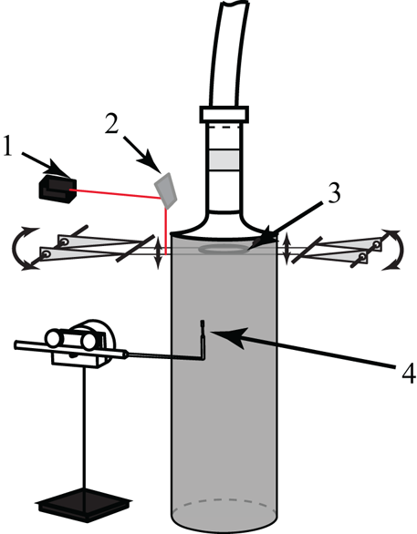
To measure the oscillating ring's displacement, we used a rangefinder (a Riftek RF603 laser triangulation sensor), shown in figure 17, with an error of measurements provided by the manufacturer of less than  ${\pm }0.25$ mm. Although this error is quite large compared with a typical ring amplitude, we always bandpass filter the data around the oscillation frequency, which removes random high-frequency noise. A comparison of the amplitude obtained by this method with direct ring amplitude measurements by a contact probe gives an amplitude error of
 ${\sim }0.04$ mm, which is acceptable for our purposes.
Rangefinder (1) and mirror (2), small oscillating ring (3) and thermoanemometer probe (4). Laser beam of the rangefinder is shown in red.

The signals of the rangefinder and the thermoanemometer were recorded synchronously, and both were bandpass filtered in a range of  ${\pm }0.5$ Hz around the ring oscillation frequency.
The correlation  $\mathrm {corr} (r,x)$ between the discrete rangefinder signal
 $s_{i}^{r}$,
 $i=0,\ldots,N-1$, and the thermoanemometer signal
 $s_{i}^{th}$,
 $i=0,\ldots,N-1$, at a given spatial point
 $(r,x)$ was calculated as
 \begin{equation} \mathrm{corr}(r,x)= \frac{ \sum _{0}^{N-1} s_i^{th} s_{i}^{r}} { \sqrt{ \sum _{0}^{N-1} (s_{i}^{th})^{2} \sum_{0}^{N-1} (s_{i}^{r})^{2}} }, \end{equation}
where  $N$ is the number of measurements during the period of 10 s. The calculation of the correlation is in fact equivalent to the phase-averaging of the anemometer signal. Indeed, for the ring oscillation
 $q = a\sin (\omega t)$ and the expected anemometer signal
 $u'=f(r) \sin (\alpha x -\omega t +\phi (r))$, we obtain, in continuous representation,
 \begin{align} \mathrm{corr}(r,x) &= \frac{ \displaystyle {\int_{0}^{T} qu' \,\textrm{d}t } }{ \displaystyle{ \sqrt{ \int_{0}^{T} u^{'2} \,\textrm{d}t \int_{0}^{T} q^{2} \,\textrm{d}t } } } \nonumber\\ &=\frac{ \displaystyle {\int_{0}^{T} \sin (\omega t) \sin (\alpha x -\omega t +\phi(r)) \,\textrm{d}t } }{ \displaystyle{ \sqrt{ \int_{0}^{T} \sin^2(\omega t) \,\textrm{d}t \int_{0}^{T} \sin^2(\alpha x -\omega t +\phi(r)) \,\textrm{d}t } } } \to - \cos (\alpha x + \phi(r)), \end{align}
as the ratio of the averaging time  $T$ to the oscillation period tends to infinity. Hence, the correlation as a function of
 $x$ for a given
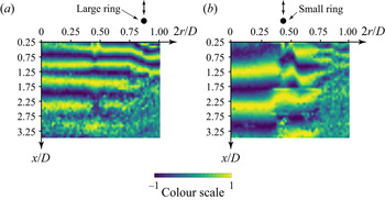
 $r$ should be a wave-like function convenient for the extraction of the wavelength. A direct phase-averaging of the anemometer signal gives the same information; however, processing the experimental data with both methods showed that the correlation analysis provides a less noisy picture, which is why we used it in the analysis below. Examples of the correlation maps in the
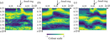
 $(r,x)$ plane are shown in figures 18 and 19, in which clear wavy structures can be seen.
Correlation maps for the signal of the rangefinder and the thermoanemometer under the action of the first (a) and the second (b) ring. The frequency of the rings' oscillations is  $6.6$ Hz.

Correlation maps for the signal of the rangefinder and the thermoanemometer under frequencies of the second ring's oscillations of (a)  $5$, (b)
 $6$ and (c)
 $7$ Hz.

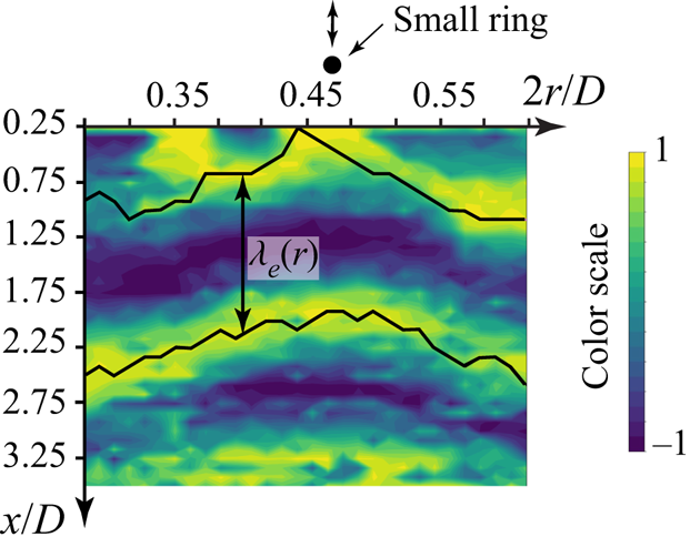
We determined the wavelengths from the image analysis of the correlation maps. Specifically, we identified two curves going in the radial direction over two successive maximums of the correlation (figure 20). Then, for each  $r$, the distance
 $\lambda _{e}(r)$ between these maximums was calculated and then radially averaged. For the first mode, for which a clear uniform wave is visible (figure 18a), the root mean square of the radial averaging is sufficiently low (
 ${<}13$ mm), but for the second mode the situation is worse. As the modes of the second branch grow much slower than those of the first branch, the excitation of the second branch is accompanied by the excitation of the first branch near the jet boundary. When moving downstream, the waves of the first branch trigger transition that occupies an increasingly large portion of the jet (figure 18b). To get rid of the first mode, we performed radial averaging in a short radial segment (figure 19). The root mean square of the calculated wavelength averaged over the frequencies analysed is
 $21$ mm, which can be regarded as the accuracy of the wavelength measurements of the second mode.
Method of wavelengths measurement: two curves going along successive maximums of the correlation, and the wavelength  $\lambda _{e}(r)$, which then was radially averaged.

4. Experimental results and comparison with theoretical predictions
4.1. Length of the laminar region
As the direct visualization shows (figure 14), the oscillations of the first ring significantly shorten the laminar region of the jet for frequencies  $\varOmega = 4 - 5.5$ Hz (
 $\omega =1 - 1.38$) that correspond to the theoretical frequency range of the fastest growing perturbations of the first branch (figure 7a). In contrast, for frequencies lower than
 $4$ Hz and greater than
 $5.5$ Hz, the effect of the ring oscillations decays with decreasing and increasing frequency, respectively. For instance, at frequencies of
 $3.5$,
 $5.75$ and
 $6.25$ Hz (figure 14), we see little impact on the jet: there are sinusoidal waves on the jet boundary, but they do not develop into Kelvin–Helmholtz billows and do not destroy the flow before the axial position at which the velocity fluctuations increase without the excitation; namely, before
 $x/D= 5$ (Zayko et al. Reference Zayko, Teplovodskii, Chicherina, Vedeneev and Reshmin2018). Note that the unperturbed jet looks laminar even at a distance of
 $6D$ from the orifice, but the velocity fluctuations are no longer small in this area. For the other frequencies shown in figure 14, there is no effect of the excitation at all.
This observation obviously suggests that faster modal growth causes earlier turbulization, which means a qualitative correlation between the theoretical and experimental growth rates. The quantitative measurements of the perturbation growth rates will be considered below.
4.2. Perturbation wavelengths
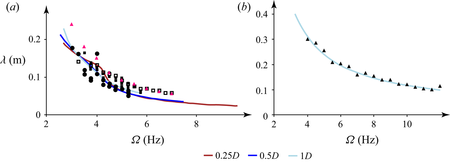
Wavelengths of the first-mode perturbations, which were obtained from the correlation maps and from the visualization, are in good agreement with each other and with the theoretically predicted wavelengths, as seen in figure 21. Note that this figure shows theoretical curves for the velocity profiles at distances  $x/D=0.25$,
 $0.5$ and
 $1$ for the first branch and at
 $x/D=0.25$,
 $0.5$,
 $1$,
 $2$ and
 $3$ for the second branch; theoretical curves for
 $x/D\le 0.1$ are not shown, because these positions are closer to the orifice than the ring (
 $\approx 0.16D$).
Comparison of the theoretical (curves; the colours correspond to the colour coding in figure 5) and experimental (markers) wavelengths of the first branch's (a) and second branch's (b) disturbances. The circles correspond to the visualization experiment with constant ring displacement amplitudes; the filled and empty squares correspond to the two series of visualization experiments with constant amplitudes of the oscillations’ velocity. The pink and black triangles are extracted from the correlation maps obtained in the experiments with the large and the small ring, respectively.

For the second branch, the theoretical wavelengths (as well as the growth rates, § 4.4) are almost independent of the distance from the orifice so that the theoretical curves calculated for all considered distances coincide with each other (see also figure 9). An excellent correlation is seen in figure 21 between the experimental points and the theoretical results for the second mode.
4.3. Radial distribution of velocity fluctuations
For  $n=0$, the amplitude
 $F$ of the axial velocity fluctuation
 $u_{x}(x,r,t)=F(r) \exp (\textrm {i}(\alpha x - \omega t))$ is expressed from the continuity equation through the radial fluctuation as (Batchelor & Gill Reference Batchelor and Gill1962)
 \begin{equation} F ={-} \frac{1}{\alpha} \left( G' + \frac{G}{r} \right). \end{equation}
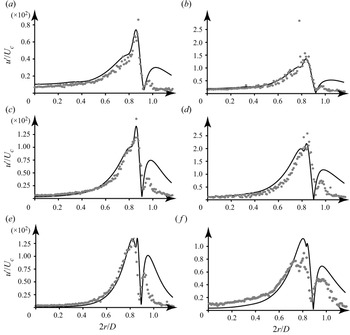
For the first branch, the experimental radial distributions of the velocity fluctuations (bandpass filtered near the value of the ring oscillation frequency) at distances  $x/D=0.5$ and
 $1$ correspond to the theoretical radial distributions of
 $|F|$, obtained in calculations with the profiles at the same distances (figure 22). The difference between the theoretical and the experimental results near the jet boundary (
 $2r/D \approx 1$) is caused by the difference between the actual velocity distribution and the unidirectional profiles used in the calculations. Indeed, as the axial velocity becomes small near the jet boundary, it becomes comparable to the radial component caused by the viscous spreading of the jet. In other words, the flow near and outside the jet boundary is two-dimensional, which is not taken into account by the theory employed. Another source of the difference is the low accuracy of thermoanemometer measurements of small velocity values. Nevertheless, inside the jet, where the flow is truly unidirectional, the correlation between the theory and the experiments is excellent.
Radial distributions of the theoretical axial amplitude  $|F|$ of the first branch's growing waves (curves) and of the velocity fluctuations
 $u'/U_{c}$ obtained in the experiments with the large ring (points). Calculations with mean profiles and similar measurements for
 $x/D = 0.5$ (a,c,e) and
 $1$ (b,d,f). Frequencies of
 $4$ (a,b),
 $5$ (c,d),
 $6.6$ (e) and
 $5.7$ (f) Hz.

For the second branch, the theoretical and experimental radial distributions of the velocity fluctuations do not agree. The reason is that the waves of the second branch are much less intense than those of the first branch due to the much lower growth rates. When the second mode is excited, the waves of the first mode are inevitably generated as well and overlap the second mode in most of the jet. This is also seen in the correlation map for the full radial range (figure 18b): upon excitation of the second mode, there is a significant change in the wavelength along the radius, whereas upon excitation of the first mode, the correlation map is rather uniform (see figure 18a).
4.4. Growth rates
For a fixed frequency, we obtain the global perturbation growth along the jet axis by the integration of local growth rates, as explained in § 2.3:
 \begin{equation} u'(x)/U_{c} = A_{0} \exp \left( \displaystyle{\int _{0}^{x} \delta(\xi)\,\textrm{d}\xi} \right) . \end{equation}
Here  $u'$ is the velocity fluctuation and
 $A_{0}$ is an arbitrary initial amplitude. We calculated the perturbation growth with
 $x$ using (4.2) for a frequency of
 $5$ Hz for the first branch and for frequencies of
 $4$,
 $5$,
 $6$,
 $8$,
 $10$ and
 $12$ Hz for the second branch.
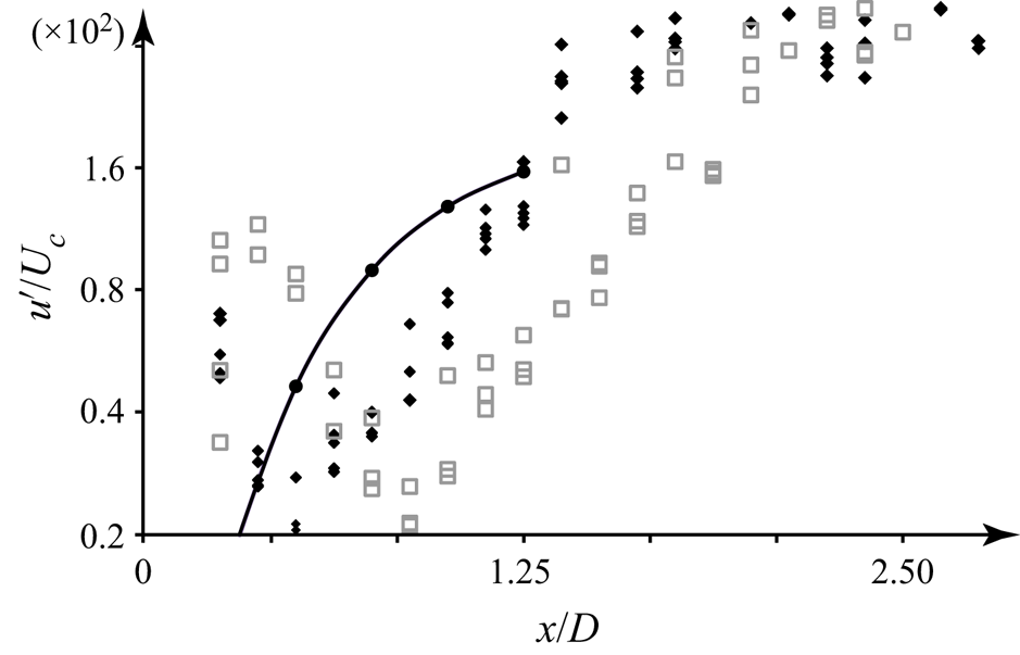
In figures 23 and 24, the theoretical growth is compared with the maximal velocity fluctuations (filtered around the ring oscillation frequency) measured in the experiments at different distances from the orifice. We observe that near the ring (within a distance  $x/D \approx$ 1), the experimental velocity fluctuation decays, because the introduced perturbation does not correspond in its spatial distribution to the growing eigenmode. After the decay of all the other spatial components, the eigenmode remains the only growing fluctuation component so that the total fluctuation starts to grow. This signifies the distance interval within which the growth rate should match the theoretical prediction. Farther downstream, after a region with a good correlation between the linear theory and the experiments, the region of linear growth of the eigenmode transforms into a region of nonlinear development that cannot be described in terms of linear stability analysis.
Theoretical growth of the first-branch mode of frequency  $5$ Hz (black circles with a solid line) and the maximal velocity fluctuations
 $u'/U_{c}$ versus
 $x/D$ in two series of experiments with the large ring (black and grey markers).

Theoretical growth of the second-branch modes (black circles with solid lines) and the maximal experimental velocity fluctuations  $u'/U_{c}$ versus
 $x/D$. Frequencies
 $4$ (a),
 $5$ (b),
 $6$ (c),
 $8$ (d),
 $10$ (e) and
 $12$ (f) Hz.

Note that constant  $A_0$ was tuned individually in each plot of figures 23 and 24 to get the eyeball correlation with the experiment in the region of linear growth. Its actual value is determined by the receptivity of the growing mode to the introduced perturbation, which is outside the scope of this study. Moreover, a change in
 $A_0$ only shifts the theoretical curve up or down but does not change the slope that drives the growth rate.
For the first branch, the experimental growth rate at a frequency of  $5$ Hz (calculated as the slope of the linear region of
 $\ln (u'/U_{c})$ as a function of
 $x$) is larger than for the second branch, which is in agreement with the theoretical predictions (figure 23). Although the experimental points of the first mode for the two series of experiments are shifted along the axis, their slopes in the linear portion are consistent with the average slope of the theoretical curve.
For the second branch (figure 24), an excellent correlation between the theory and the experiments in a certain range of axial positions is also clear. The inclination of the linear region of the function  $\ln (u'/U_{c})$ decreases with an increase in the frequency of the disturbance from
 $5$ to
 $12$ Hz (figure 24), which is also in agreement with the theoretical results.
5. Conclusions
In this paper, we have experimentally studied the development of small controlled axisymmetric perturbations in a laminar jet at  $Re = 5400$. The jet has two axisymmetric modes of instability, which were studied separately. We analysed the first mode, which is localized near a jet boundary, by flow visualization in a laser sheet and thermoanemometer measurements. The internal inflection point generates the second mode, which was studied by correlation analysis between thermoanemometer measurements and the vibrating ring. The results are compared with eigenmode calculations of the Rayleigh equation with the parallel-flow assumption. We have shown that the wavelengths and growth rates of both modes, as well as the perturbation velocity profiles of the first mode, are in excellent agreement with theoretical analysis. Unlike previous studies, we considered only the truly laminar portion of the jet, and the perturbations in our experiment are truly small and have a significant region of exponential evolution downstream; in this sense, our study is the first fair validation of inviscid stability theory for a jet flow. A good correlation between experimental and theoretical data somewhat closes the question on the role of nonlinear mechanisms in the initial evolution of jet perturbations; at least at quiet conditions, strong inviscid instability develops purely linearly.
Our results prove that linear inviscid stability theory with a unidirectional-flow approximation is a robust tool for the analysis and optimization of high-Reynolds-number laminar jet flows in ‘quiet’ ambient conditions, even when taking into account slow jet evolution due to viscous spreading. We believe that further analysis of perturbation growth under other conditions, including receptivity analysis and non-modal transition, will result in the development of new methods for jet transition control, which are currently quite mature for wall-bounded flows but do not have their analogues for open flows. Also, as there is growing evidence that linear mechanisms play a crucial role in sustaining large-scale structures in fully turbulent jets, a firm basis for linear stability theory will clearly be useful for their analysis.
We expect that the growth of perturbations according to inviscid linear stability theory, as demonstrated in this study in a laminar jet, can also occur in other open flows, such as wakes and free shear layers, for which the instability mechanism, namely inviscid instability generated by an inflection point of the velocity profile, is similar to that of jets.
Funding
This work is supported by the Russian Science Foundation under grant 20-19-00404.
Declaration of interests
The authors report no conflict of interest.