1 Introduction
In recent years, many researchers have been interested in the dusty plasma because it is different from the typical two-component electron–ion plasma and has many applications (Fortov & Morfill Reference Fortov and Morfill2009). In a dusty plasma, nano-micron-sized dust particles are immersed in an ionized gas composed of electrons and ions, and collide with electrons and ions, becoming charged, a process which we can observe in many environments, including low temperature laboratory plasmas used for tools and processing, space plasmas (e.g. noctilucent clouds, comet tails, planetary rings) (Goertz Reference Goertz1989; Mendis & Rosenberg Reference Mendis and Rosenberg1994) and plasma crystals (Dresselhaus, Kip & Kittel Reference Dresselhaus, Kip and Kittel1955) or Coulomb lattices (Melzer, Trottenberg & Piel Reference Melzer, Trottenberg and Piel1994) of charged dust grains in plasmas. The presence of highly negatively charged dust particles in the plasma can alter the collective behaviour of the plasma and stimulate new modes and new nonlinear phenomena, for example dust-ion-acoustic waves (Shukla & Silin Reference Shukla and Silin1992), dust-acoustic (DA) waves (Rao, Shukla & Yu Reference Rao, Shukla and Yu1990), dust lattice waves (MelandsØ Reference MelandsØ1996), dust Coulomb waves (Rao Reference Rao1999), dust voids (Samsonov & Goree Reference Samsonov and Goree1999), etc.
Interaction between solitary waves is a hot topic in the field of nonlinear physics (Korteweg & de Vries Reference Korteweg and de Vries1895; Zabusky & Kruskal Reference Zabusky and Kruskal1965; Heidemann et al. Reference Heidemann, Zhdanov, Sutterlin, Thomas and Morfill2009; Mamun & Shukla Reference Mamun and Shukla2009). In a one-dimensional system, there are two different interaction processes. One is the overtaking collision, which can be investigated by the inverse scattering transform method (Gardner et al. Reference Gardner, Greener, Kruskal and Miura1967), and the other is the head-on collision (Su & Mirie Reference Su and Mirie1980), where the angle between the two soliton propagation directions is  $\unicode[STIX]{x03C0}$. For the head-on collision between two solitary waves, one of interesting questions regards the phase shift after collision, which has been extensively studied by using the Poincaré–Lighthill–Kuo (PLK) method (Jeffery & Kawahawa Reference Jeffery and Kawahawa1982; Huang & Velarde Reference Huang and Velarde1996; Xue Reference Xue2004; Han et al. Reference Han, Yang, Tian and Duan2008; Verheest, Hellberg & Hereman Reference Verheest, Hellberg and Hereman2012; Zhang et al. Reference Zhang, Yang, Xu, Yang, Qi and Duan2014).
As is well known, charged dust particles are usually exposed to electrostatic forces from adjacent dust particles. Because of the high charge and low temperature on dust particles, they can easily enter the strong coupling state, which was theoretically predicted by Ikezi (Reference Ikezi1986) several decades ago. The larger the charge of the dust particles, the higher the potential energy between the particles and the surrounding particles. The ratio of potential energy to kinetic energy is usually used to reflect the coupling parameter  $\unicode[STIX]{x1D6E4}$, which measures the relative importance of these electrostatic forces to the kinetic energy of the dust particles (Ghosh et al. Reference Ghosh, Gupta, Chakrabarti and Chaudhuri2011; Cousens et al. Reference Cousens, Yaroshenko, Sultana, Hellberg, Verheest and Kourakis2014). In a strongly coupled dusty plasma (
 $\unicode[STIX]{x1D6E4}\gg 1$), experimental results (Thomas & Morfill Reference Thomas and Morfill1996) show the existence of liquid or solid-like behaviour of the dusty plasma medium. It is found that the crystal–liquid phase transition occurs when the coupling parameter is greater than its critical value, i.e.
 $\unicode[STIX]{x1D6E4}>\unicode[STIX]{x1D6E4}_{c}$. In a strongly coupled dusty plasma, the nonlinear coherent structures are extensively investigated theoretically (Mishra, Kaw & Sen Reference Mishra, Kaw and Sen2000; Xie & Yu Reference Xie and Yu2000; Mamun, Ashrafi & Shukla Reference Mamun, Ashrafi and Shukla2010; Veeresha et al. Reference Veeresha, Tiwari, Sen, Kaw and Das2010; El-Labany et al. Reference El-Labany, El-Taibany, El-Shamy, El-Depsy and Zedan2012; EL-Shamy & Al-Asbali Reference EL-Shamy and Al-Asbali2014; Borah, Bhattacharjee & Das Reference Borah, Bhattacharjee and Das2016; Shahmansouri & Mamun Reference Shahmansouri and Mamun2015), experimentally (Thomas & Morfill Reference Thomas and Morfill1996; Nosenko, Goree & Piel Reference Nosenko, Goree and Piel2006; Sheridan, Nosenko & Goree Reference Sheridan, Nosenko and Goree2008; Sharma, Boruah & Bailung Reference Sharma, Boruah and Bailung2014) and numerically (Cousens et al. Reference Cousens, Yaroshenko, Sultana, Hellberg, Verheest and Kourakis2014; Tiwari et al. Reference Tiwari, Das, Sen and Kaw2015; Kumar, Tiwari & Das Reference Kumar, Tiwari and Das2017). Mishra et al. (Reference Mishra, Kaw and Sen2000), and Nosenko et al. (Reference Nosenko, Goree and Piel2006) studied the stability and propagation of shear waves in a strongly coupled dusty plasma. The effects of the polarization force and effective electron temperature on shock waves is studied by Mamun et al. (Reference Mamun, Ashrafi and Shukla2010). The increasing acoustic shock speed due to strong coupling (EL-Shamy & Al-Asbali Reference EL-Shamy and Al-Asbali2014) and the influence of the dust kinematic viscosity on the shock wave trajectory after collision in a strongly coupled dusty plasma (Cousens et al. Reference Cousens, Yaroshenko, Sultana, Hellberg, Verheest and Kourakis2014) have also been investigated. Many researchers (Xie & Yu Reference Xie and Yu2000; Veeresha et al. Reference Veeresha, Tiwari, Sen, Kaw and Das2010; El-Labany et al. Reference El-Labany, El-Taibany, El-Shamy, El-Depsy and Zedan2012) have studied DA waves in a strongly coupled complex plasma. Other authors (Sheridan et al. Reference Sheridan, Nosenko and Goree2008; Sharma et al. Reference Sharma, Boruah and Bailung2014; Tiwari et al. Reference Tiwari, Das, Sen and Kaw2015) have investigated the phase shift for the collisions between solitons and the characteristics of a solitary wave in a strongly coupled complex plasma. The interaction of flowing particles (Shahmansouri & Mamun Reference Shahmansouri and Mamun2015) and the electrostatic forces (Borah et al. Reference Borah, Bhattacharjee and Das2016) of the dust particles can affect the isolated structure in a strongly coupled dusty plasma.
Although many authors (Jaiswal, Bandyopadhyay & Sen Reference Jaiswal, Bandyopadhyay and Sen2014; Sharma et al. Reference Sharma, Boruah and Bailung2014) have studied the head-on collision between two solitary waves of a strongly coupled dusty plasma theoretically and experimentally, the application scope of the PLK to solving the head-on collision is still lacking. The present paper tries to answer this question by using the particle-in-cell (PIC) simulation method. The effects of the coupling parameters on both the head-on collision and the waveform are also studied in the present paper.
2 Theoretical model and PIC method
Dust dynamics is of great importance and can be used to study low frequency phenomena ( $\unicode[STIX]{x1D714}\ll k\unicode[STIX]{x1D710}_{\text{the}},k\unicode[STIX]{x1D710}_{\text{thi}}$, where
 $k$,
 $\unicode[STIX]{x1D714}$,
 $\unicode[STIX]{x1D710}_{\text{the}}$ and
 $\unicode[STIX]{x1D710}_{\text{thi}}$ are the wavenumber, the mode frequency, the electronic thermal velocity and the ionic thermal velocity, respectively) in dusty plasmas. We assume that both ions and electrons are inertial so that they satisfy the Boltzmann distribution as follows:
 $$\begin{eqnarray}\displaystyle & \displaystyle n_{e}=n_{e0}\exp \left(\frac{e\unicode[STIX]{x1D719}}{T_{e}}\right), & \displaystyle\end{eqnarray}$$
 $$\begin{eqnarray}\displaystyle & \displaystyle n_{i}=n_{i0}\exp \left(\frac{e\unicode[STIX]{x1D719}}{T_{i}}\right), & \displaystyle\end{eqnarray}$$
where  $n_{e0}$ and
 $n_{i0}$ are the unperturbed number densities of electrons and ions,
 $T_{e}$ and
 $T_{i}$ are the electron and ion temperatures,
 $\unicode[STIX]{x1D719}$ is the static electric potential,
 $e$ is the charge per unit electron.
The dusty plasm we consider in the present paper is an unmagnetized collisionless three-component system, namely electrons, ions and dust particles. We assume that dust particles are strongly coupled due to their high charge and low temperature and the dust dynamics is essentially adiabatic ( $\unicode[STIX]{x1D714}\gg k\unicode[STIX]{x1D710}_{\text{thd}}$, where
 $\unicode[STIX]{x1D710}_{\text{thd}}$ is the dust thermal velocity). We describe the dynamics of strongly coupled dust particles by using the generalized hydrodynamic model, introducing a viscoelastic effect and compressibility. The change of dispersion due to the strong coupling effect is mainly caused by compressibility, so we ignore the dissipation caused by viscosity and dust collisions. The neglect of dissipative effects is a valid approximation in the modes with
 $\unicode[STIX]{x1D714}\unicode[STIX]{x1D70F}_{m}\gg 1$, the so-called kinetic modes, where
 $\unicode[STIX]{x1D70F}_{m}$ is the relaxation (memory) time. Therefore, the dynamics of the dust fluid in such a strongly coupled dusty plasma is governed as follows (Jaiswal et al. Reference Jaiswal, Bandyopadhyay and Sen2014):
 $$\begin{eqnarray}\displaystyle & \displaystyle \frac{\unicode[STIX]{x2202}n_{d}}{\unicode[STIX]{x2202}t}+\frac{\unicode[STIX]{x2202}(n_{d}u_{d})}{\unicode[STIX]{x2202}x}=0, & \displaystyle\end{eqnarray}$$
 $$\begin{eqnarray}\displaystyle & \displaystyle \frac{\unicode[STIX]{x2202}u_{d}}{\unicode[STIX]{x2202}t}+u_{d}\frac{\unicode[STIX]{x2202}n_{d}}{\unicode[STIX]{x2202}x}=\frac{\unicode[STIX]{x2202}\unicode[STIX]{x1D719}}{\unicode[STIX]{x2202}x}-\frac{\unicode[STIX]{x1D6FE}^{\prime }}{n_{d}}\frac{\unicode[STIX]{x2202}n_{d}}{\unicode[STIX]{x2202}x}, & \displaystyle\end{eqnarray}$$
 $$\begin{eqnarray}\displaystyle & \displaystyle \frac{\unicode[STIX]{x2202}^{2}\unicode[STIX]{x1D719}}{\unicode[STIX]{x2202}x^{2}}=n_{d}+\unicode[STIX]{x1D708}\text{e}^{\unicode[STIX]{x1D6FD}s\unicode[STIX]{x1D719}}-\unicode[STIX]{x1D707}\text{e}^{-s\unicode[STIX]{x1D719}}, & \displaystyle\end{eqnarray}$$
where  $\unicode[STIX]{x1D708}$ and
 $\unicode[STIX]{x1D707}$ are the ion and electron number densities expressed as
 $\unicode[STIX]{x1D707}=n_{i0}/(n_{i0}-n_{e0})$ and
 $\unicode[STIX]{x1D708}=n_{e0}/(n_{i0}-n_{e0})$. Here,
 $\unicode[STIX]{x1D6FD}=T_{i}/T_{e}$ is the ratio of the ion and electron temperatures,
 $s=1/(\unicode[STIX]{x1D707}+\unicode[STIX]{x1D708}\unicode[STIX]{x1D6FD})$. Moreover, the following dimensionless variables are adopted:
 $x\rightarrow x/\unicode[STIX]{x1D706}_{d}$,
 $u_{d}\rightarrow u_{d}/C_{d}$,
 $t\rightarrow t/\unicode[STIX]{x1D714}_{pd}^{-1}$,
 $\unicode[STIX]{x1D719}\rightarrow \unicode[STIX]{x1D719}e/T_{\text{eff}}$ and
 $n_{d}\rightarrow n_{d}/n_{d0}$, where
 $\unicode[STIX]{x1D706}_{d}=(\text{Teff}/4\unicode[STIX]{x03C0}Z_{d}n_{d0}e^{2})^{1/2}$,
 $C_{d}=(Z_{d}T_{\text{eff}}/m_{d})^{1/2}$,
 $\unicode[STIX]{x1D714}_{pd}=(4\unicode[STIX]{x03C0}n_{d0}Z_{d}^{2}e^{2}/m_{d})^{1/2}$ and
 $T_{\text{eff}}=T_{i}T_{e}/(\unicode[STIX]{x1D707}T_{e}+\unicode[STIX]{x1D708}T_{i})$ are the Debye length, sound speed, frequency and effective temperature of the dusty plasma, respectively;
 $Z_{d}$ is the charge number residing on the dust grain measured in units of electron charge
 $e$;
 $n_{d}$,
 $u_{d}$ and
 $m_{d}$ are the number density, velocity and the mass of the dust grains,
 $n_{d0}$ is the unperturbed number density of dust grains,
 $\unicode[STIX]{x1D6FE}^{\prime }=\unicode[STIX]{x1D6FE}T_{d}/Z_{d}T_{i}$, where
 $\unicode[STIX]{x1D6FE}$ is the compressibility and
 $T_{d}$ denotes the dust temperature. We neglect any charge fluctuation of dust fluid in our model. The compressibility is defined as follows (Kaw & Sen Reference Kaw and Sen1998):
 $$\begin{eqnarray}\unicode[STIX]{x1D6FE}=\frac{1}{T_{d}}\left(\frac{\unicode[STIX]{x2202}P}{\unicode[STIX]{x2202}n}\right)_{T_{d}}=1+\frac{u(\unicode[STIX]{x1D6E4})}{3}+\frac{\unicode[STIX]{x1D6E4}}{9}\frac{\unicode[STIX]{x2202}u(\unicode[STIX]{x1D6E4})}{\unicode[STIX]{x2202}\unicode[STIX]{x1D6E4}},\end{eqnarray}$$
where  $u(\unicode[STIX]{x1D6E4})$ is the free energy of the system, given by Slattery, Doolen & DeWitt (Reference Slattery, Doolen and DeWitt1980, Reference Slattery, Doolen and DeWitt1982)
 $$\begin{eqnarray}u(\unicode[STIX]{x1D6E4})=-0.89\unicode[STIX]{x1D6E4}+0.95\unicode[STIX]{x1D6E4}^{-1/4}+0.19\unicode[STIX]{x1D6E4}^{-1/4}-0.81.\end{eqnarray}$$
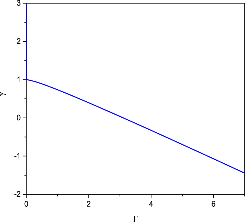
Figure 1 shows the dependence of  $\unicode[STIX]{x1D6FE}$ on the parameter
 $\unicode[STIX]{x1D6E4}$. Notice that
 $\unicode[STIX]{x1D6FE}$ decreases as
 $\unicode[STIX]{x1D6E4}$ increases. In a weakly coupled state (
 $\unicode[STIX]{x1D6E4}<1$),
 $\unicode[STIX]{x1D6FE}$ is positive, but it becomes negative as
 $\unicode[STIX]{x1D6E4}$ increases, which corresponds to the liquid state.
The dependence of  $\unicode[STIX]{x1D6FE}$ on the parameter
 $\unicode[STIX]{x1D6E4}$.

Now, we consider the head-on collision between two oppositely propagating Korteweg–de Vries (KdV) solitary waves 1 and 2. Initially, they are far apart and they propagate towards each other. After some time, they interact and have a head-on collision. In order to study this process, we adopt the PLK method in the limit of the long wavelength and small amplitude wave approximation. We introduce the following stretched coordinates:
 $$\begin{eqnarray}\displaystyle & \displaystyle \unicode[STIX]{x1D709}=\unicode[STIX]{x1D700}(kx-\unicode[STIX]{x1D706}t)+\unicode[STIX]{x1D700}^{2}P_{0}(\unicode[STIX]{x1D702},\unicode[STIX]{x1D70F})+\unicode[STIX]{x1D700}^{3}P_{1}(\unicode[STIX]{x1D702},\unicode[STIX]{x1D70F})+\cdots , & \displaystyle\end{eqnarray}$$
 $$\begin{eqnarray}\displaystyle & \displaystyle \unicode[STIX]{x1D702}=\unicode[STIX]{x1D700}(kx+\unicode[STIX]{x1D706}t)+\unicode[STIX]{x1D700}^{2}Q_{0}(\unicode[STIX]{x1D709},\unicode[STIX]{x1D70F})+\unicode[STIX]{x1D700}^{3}Q_{1}(\unicode[STIX]{x1D709},\unicode[STIX]{x1D70F})+\cdots , & \displaystyle\end{eqnarray}$$
 $$\begin{eqnarray}\displaystyle & \displaystyle \unicode[STIX]{x1D70F}=\unicode[STIX]{x1D700}^{3}t, & \displaystyle\end{eqnarray}$$
where  $\unicode[STIX]{x1D709}$ and
 $\unicode[STIX]{x1D702}$ represent the coordinates of the trajectories of the two solitary waves traveling to the right and the left, respectively,
 $\unicode[STIX]{x1D706}$ is the speed of a linear DA solitary wave. The associated variables are expanded around the equilibrium values in powers of
 $\unicode[STIX]{x1D700}$ as follows:
 $$\begin{eqnarray}\displaystyle & \displaystyle n_{d}=1+\unicode[STIX]{x1D700}^{2}n_{1}+\unicode[STIX]{x1D700}^{4}n_{2}+\cdots & \displaystyle\end{eqnarray}$$
 $$\begin{eqnarray}\displaystyle & \displaystyle u_{d}=\unicode[STIX]{x1D700}^{2}u_{1}+\unicode[STIX]{x1D700}^{4}u_{2}+\cdots & \displaystyle\end{eqnarray}$$
 $$\begin{eqnarray}\displaystyle & \displaystyle \unicode[STIX]{x1D719}=\unicode[STIX]{x1D700}^{2}\unicode[STIX]{x1D719}_{1}+\unicode[STIX]{x1D700}^{4}\unicode[STIX]{x1D719}_{2}+\cdots . & \displaystyle\end{eqnarray}$$
Substituting (2.11)–(2.13) into (2.3)–(2.5) and following the previous technique (Xue Reference Xue2004; Jaiswal et al. Reference Jaiswal, Bandyopadhyay and Sen2014; Zhang et al. Reference Zhang, Yang, Xu, Yang, Qi and Duan2014), we obtain, at the lowest order:  $\unicode[STIX]{x1D719}_{1}(\unicode[STIX]{x1D709},\unicode[STIX]{x1D702},\unicode[STIX]{x1D70F})=\unicode[STIX]{x1D6F7}_{1}(\unicode[STIX]{x1D709},\unicode[STIX]{x1D70F})+\unicode[STIX]{x1D6F7}_{2}(\unicode[STIX]{x1D702},\unicode[STIX]{x1D70F})$,
 $n_{1}(\unicode[STIX]{x1D709},\unicode[STIX]{x1D702},\unicode[STIX]{x1D70F})=1-[\unicode[STIX]{x1D6F7}_{1}(\unicode[STIX]{x1D709},\unicode[STIX]{x1D70F})+\unicode[STIX]{x1D6F7}_{2}(\unicode[STIX]{x1D702},\unicode[STIX]{x1D70F})]$,
 $u_{1}(\unicode[STIX]{x1D709},\unicode[STIX]{x1D702},\unicode[STIX]{x1D70F})=-\unicode[STIX]{x1D706}[\unicode[STIX]{x1D6F7}_{1}(\unicode[STIX]{x1D709},\unicode[STIX]{x1D70F})-\unicode[STIX]{x1D6F7}_{2}(\unicode[STIX]{x1D702},\unicode[STIX]{x1D70F})]$ and
 $\unicode[STIX]{x1D706}=\sqrt{1+\unicode[STIX]{x1D6FE}^{\prime }}$.
For the next lowest-order terms, we obtain the KdV equations
 $$\begin{eqnarray}\displaystyle & \displaystyle \frac{\unicode[STIX]{x2202}\unicode[STIX]{x1D6F7}_{1}}{\unicode[STIX]{x2202}\unicode[STIX]{x1D70F}}+a\unicode[STIX]{x1D6F7}_{1}\frac{\unicode[STIX]{x2202}\unicode[STIX]{x1D6F7}_{1}}{\unicode[STIX]{x2202}\unicode[STIX]{x1D709}}+b\frac{\unicode[STIX]{x2202}^{3}\unicode[STIX]{x1D6F7}_{1}}{\unicode[STIX]{x2202}\unicode[STIX]{x1D709}^{3}}=0, & \displaystyle\end{eqnarray}$$
 $$\begin{eqnarray}\displaystyle & \displaystyle \frac{\unicode[STIX]{x2202}\unicode[STIX]{x1D6F7}_{2}}{\unicode[STIX]{x2202}\unicode[STIX]{x1D70F}}-a\unicode[STIX]{x1D6F7}_{2}\frac{\unicode[STIX]{x2202}\unicode[STIX]{x1D6F7}_{2}}{\unicode[STIX]{x2202}\unicode[STIX]{x1D702}}-b\frac{\unicode[STIX]{x2202}^{3}\unicode[STIX]{x1D6F7}_{2}}{\unicode[STIX]{x2202}\unicode[STIX]{x1D702}^{3}}=0, & \displaystyle\end{eqnarray}$$
where  $a=-(1/2\unicode[STIX]{x1D706})[3+s^{2}(\unicode[STIX]{x1D6FD}^{2}\unicode[STIX]{x1D708}-\unicode[STIX]{x1D707})+2\unicode[STIX]{x1D6FE}^{\prime }]$, and
 $b=1/2\unicode[STIX]{x1D706}$.
The solitary wave solutions of (2.14) and (2.15) are
 $$\begin{eqnarray}\displaystyle & \displaystyle \unicode[STIX]{x1D6F7}_{1}=\frac{3u_{0}}{a}\text{Sech}^{2}\left[\frac{\unicode[STIX]{x1D709}-u_{0}\unicode[STIX]{x1D70F}+\unicode[STIX]{x1D6FF}_{A}}{2\sqrt{{\displaystyle \frac{b}{u_{0}}}}}\right], & \displaystyle\end{eqnarray}$$
 $$\begin{eqnarray}\displaystyle & \displaystyle \unicode[STIX]{x1D6F7}_{2}=\frac{3u_{0}}{a}\text{Sech}^{2}\left[\frac{\unicode[STIX]{x1D702}+u_{0}\unicode[STIX]{x1D70F}+\unicode[STIX]{x1D6FF}_{B}}{2\sqrt{{\displaystyle \frac{b}{u_{0}}}}}\right], & \displaystyle\end{eqnarray}$$
where  $u_{0}$ is a constant,
 $\unicode[STIX]{x1D6FF}_{A}$ and
 $\unicode[STIX]{x1D6FF}_{B}$ are the initial phases of the two solitary waves.
The phase shifts of solitary wave  $1$ and solitary wave
 $2$ are
 $$\begin{eqnarray}\displaystyle & \displaystyle \unicode[STIX]{x0394}x_{A}=-\frac{3\unicode[STIX]{x1D700}}{a(1+\unicode[STIX]{x1D6FE}^{\prime })}\sqrt{bu_{0}}[-1-2\unicode[STIX]{x1D6FE}^{\prime }+s^{2}(\unicode[STIX]{x1D6FD}^{2}\unicode[STIX]{x1D708}-\unicode[STIX]{x1D707})] & \displaystyle\end{eqnarray}$$
 $$\begin{eqnarray}\displaystyle & \displaystyle \unicode[STIX]{x0394}x_{B}=\frac{3\unicode[STIX]{x1D700}}{a(1+\unicode[STIX]{x1D6FE}^{\prime })}\sqrt{bu_{0}}[-1-2\unicode[STIX]{x1D6FE}^{\prime }+s^{2}(\unicode[STIX]{x1D6FD}^{2}\unicode[STIX]{x1D708}-\unicode[STIX]{x1D707})]. & \displaystyle\end{eqnarray}$$
Although the head-on collision of two solitary waves has been studied (Xue Reference Xue2004; Zhang et al. Reference Zhang, Yang, Xu, Yang, Qi and Duan2014), the present study will use the PIC simulation method to study this process in a strongly coupled dusty plasma. The comparisons between the analytical results and the numerical ones are given. Then, the application scope of the PLK method is given for the head-on collision between two solitary waves for a strongly coupled dusty plasma. In the process of simulation, the dust particles are represented as so-called super-particles (SPs), while electrons and ions are modelled as a Boltzmann distributed background. The motion of the SPs replaces the actual charged plasma particles, while each SP has a weight factor,  $S$, specifying the number of real particles contained. In PIC simulation, the simulation area is divided into multiple grid cells. At each time step, we weigh the position and velocity of the SPs on the grid to obtain the charge density. Once the charge density is obtained, Poisson’s equation is used to solve the potential of each grid, and the electric field (
 $E$) is further derived. Then, each SP motion is driven by the electric field, and the new position and velocity are obtained by the motion equation. The equation of motion of the system is Newton’s equation
 $$\begin{eqnarray}m_{d}\frac{\text{d}u}{\text{d}t}=-Eq-\frac{\unicode[STIX]{x1D6FE}^{\prime }}{n_{d}}\frac{\unicode[STIX]{x2202}n_{d}}{\unicode[STIX]{x2202}x}.\end{eqnarray}$$
In the PIC simulation, the initial conditions are given as follows:  $\unicode[STIX]{x1D719}=\unicode[STIX]{x1D6F7}_{1}^{\prime }+\unicode[STIX]{x1D6F7}_{2}^{\prime }$,
 $n_{d}=1-(\unicode[STIX]{x1D6F7}_{1}^{\prime }+\unicode[STIX]{x1D6F7}_{2}^{\prime })$ and
 $u_{d}=-\unicode[STIX]{x1D706}(\unicode[STIX]{x1D6F7}_{1}^{\prime }-\unicode[STIX]{x1D6F7}_{2}^{\prime })$, where
 $\unicode[STIX]{x1D6F7}_{1}^{\prime }=(3u_{0}\unicode[STIX]{x1D700}^{2}/a)\text{Sech}^{2}[\unicode[STIX]{x1D700}((x-(1+u_{0}\unicode[STIX]{x1D700}^{2})t+\unicode[STIX]{x1D6FF}_{A}])/(2\sqrt{b/u_{0}}))$ and
 $\unicode[STIX]{x1D6F7}_{2}^{\prime }=(3u_{0}\unicode[STIX]{x1D700}^{2}/a)\text{Sech}^{2}[\unicode[STIX]{x1D700}((x+(1+u_{0}\unicode[STIX]{x1D700}^{2})t+\unicode[STIX]{x1D6FF}_{B})/(2\sqrt{b/u_{0}}))]$. Fixed boundary conditions are chosen. The parameters in the simulation are as follows: grid size
 $\text{d}x=0.05$, number of grid cell
 $N_{x}=30\,000$, time step
 $\text{d}t=0.002$, total length of
 $x$-axis
 $L_{x}=\text{d}xN_{x}$,
 $S=50$,
 $\unicode[STIX]{x1D707}=1.1$,
 $\unicode[STIX]{x1D708}=0.1$,
 $\unicode[STIX]{x1D6FD}=0.1$ and
 $u_{0}=1$.
3 Results and discussion
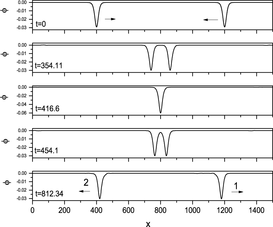
Figure 2 shows the process of a head-on collision between two solitary waves with the same amplitude, where  $\unicode[STIX]{x1D700}=0.1$,
 $\unicode[STIX]{x1D6FE}=-10$. It shows that the waveform and the propagation speed of two solitary waves remain unchanged after the head-on collision, meaning that the propagation of the soliton is relatively stable. It is also found that the maximum amplitude during the collision is approximately the sum of the two initial amplitudes.
The time evolution of two colliding solitary waves in coming from opposite directions, where  $\unicode[STIX]{x1D700}=0.1$,
 $\unicode[STIX]{x1D6FE}=-10$.

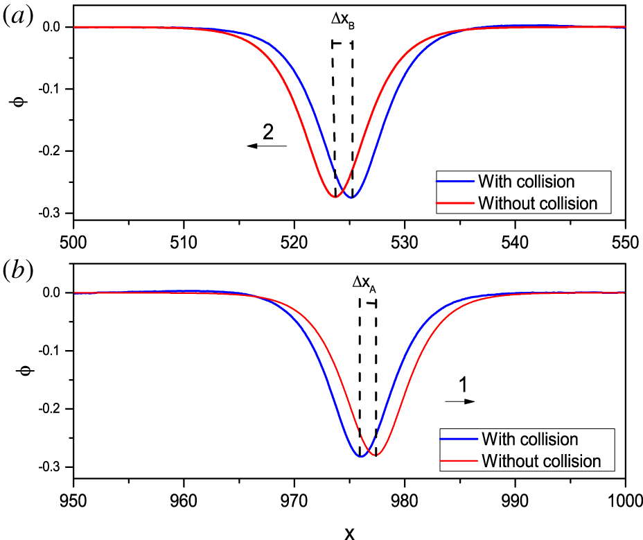
The definition of the phase shift caused by the head-on collision between two solitary waves, (a) profile of solitary wave 2, (b) profile of solitary wave 1. The red line represents the waveform without a collision, while the blue line represents the waveform after the head-on collision at the same time, where  $\unicode[STIX]{x1D700}=0.3$,
 $\unicode[STIX]{x1D6FE}=-10$.

Figure 3 shows the phase shift of solitary waves caused by the collision of two solitary waves, where  $\unicode[STIX]{x1D700}=0.3$,
 $\unicode[STIX]{x1D6FE}=-10$. Figure 3(a) is the comparisons of the waveform of the solitary wave 2 between that after head-on collision and that without collision. Figure 3(b) is for the solitary wave 1. The red line is that without collision at
 $t=833.2$, while the blue line is that with collision at
 $t=833.2$. A phase shift for both solitary waves is obviously observed in figure 3, as reported in Jaiswal et al. (Reference Jaiswal, Bandyopadhyay and Sen2014). The negative phase shift means that the velocity of each soliton decreases during the head-on collision.
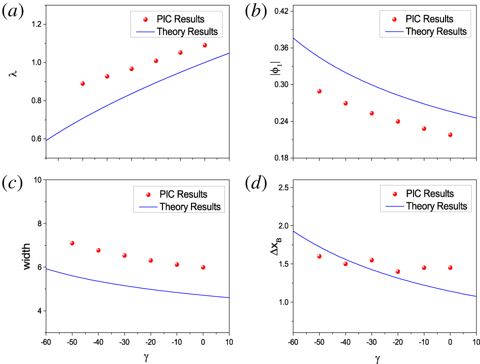
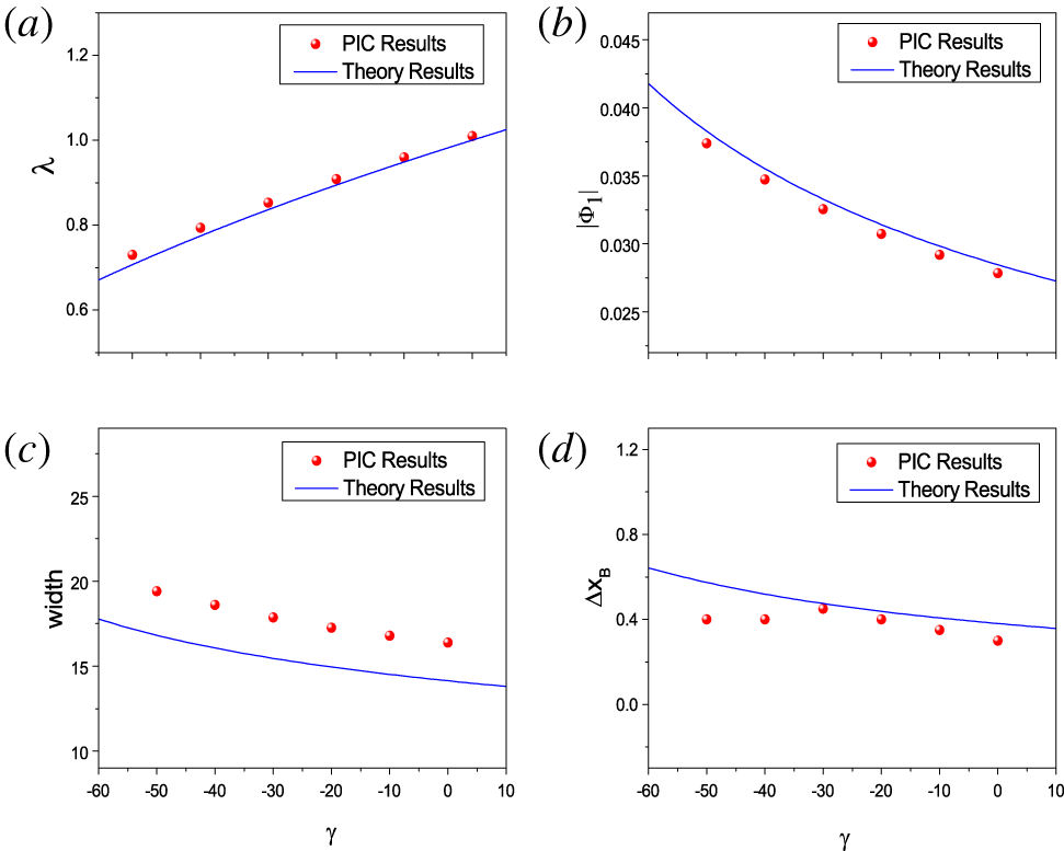
The dependence of the speed, the amplitude and the width of solitary wave 1 on the parameter  $\unicode[STIX]{x1D6FE}$, shown in (a), (b) and (c), respectively. The dependence of the phase shift of solitary wave 2 of the head-on collision between two solitary waves on
 $\unicode[STIX]{x1D6FE}$ in (d). The solid blue line represents the analytical results, while the red dots represent the numerical ones, where
 $\unicode[STIX]{x1D700}=0.3$.

In order to understand the effect of the coupling parameter  $\unicode[STIX]{x1D6E4}$, figure 4(a) shows the dependence of the wave speed on
 $\unicode[STIX]{x1D6FE}$. Comparisons between the numerical results and the analytical ones are given. Notice that the propagation speed increases as the compressibility (
 $\unicode[STIX]{x1D6FE}$) increases. It seems that differences between the numerical results and the analytical ones decreases as the coupling parameter increases. Figure 4(b) shows the dependence of the wave amplitude on
 $\unicode[STIX]{x1D6FE}$. Comparisons between the numerical results and the analytical ones are also shown. It indicates that the wave amplitude decreases as the compressibility increases. Figure 4(c) shows the dependence of the wave width on
 $\unicode[STIX]{x1D6FE}$. Both the numerical results and the analytical ones are given. It seems that the wave width decreases as the compressibility increases. We are interested in how the coupling strength between dusty grains affects the phase shift of solitary waves after a head-on collision. For this purpose, figure 4(d) shows the phase shift of solitary wave 2 as a function of
 $\unicode[STIX]{x1D6FE}$. Both the numerical results and the analytical ones are shown in figure 4(d). It is observed that the phase shift decreases as the compressibility increases. In other words, as compressibility decreases, the coupling strength increases.
The dependence of the speed, the amplitude and the width of solitary wave 2 on the parameter  $\unicode[STIX]{x1D6FE}$, shown in (a), (b) and (c), respectively. The dependence of the phase shift of solitary wave 2 of the head-on collision between two solitary waves on
 $\unicode[STIX]{x1D6FE}$ in (d). The solid blue line represents the analytical results, while the red dots represent the numerical ones, where
 $\unicode[STIX]{x1D700}=0.1$.

Similar to figure 4, the dependences of the speed, amplitude, width and phase shift on  $\unicode[STIX]{x1D6FE}$ after a collision between two waves are shown in figure 5, where
 $\unicode[STIX]{x1D700}=0.1$. Compared with figure 4, notice that the differences between the analytical results and the numerical ones when
 $\unicode[STIX]{x1D700}=0.1$ are less than when
 $\unicode[STIX]{x1D700}=0.3$. It seems that the lower
 $\unicode[STIX]{x1D700}$, the smaller the difference between the analytical results and the numerical ones.
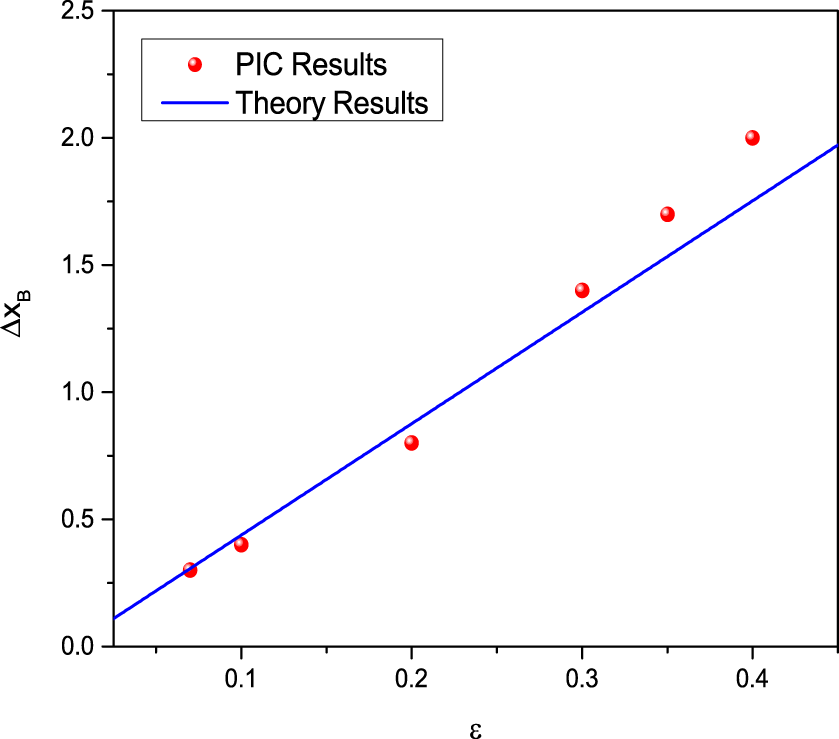
The dependence of the phase shift of solitary wave 2 after the head-on collision between solitary wave 1 and 2 on  $\unicode[STIX]{x1D700}$. The solid blue line represents the analytical results, while the red dots represent the numerical ones, where
 $\unicode[STIX]{x1D6FE}=-20$.

Figure 6 shows the dependence of the phase shift of solitary wave 2 on the parameter  $\unicode[STIX]{x1D700}$, where
 $0<\unicode[STIX]{x1D700}\leqslant 0.4$. Notice that the smaller
 $\unicode[STIX]{x1D700}$, the smaller the differences between the numerical results and the analytical ones. We infer that the analytical results are only valid for small amplitude waves.
It is found that the dust pressure has an effect on the head-on collision between two solitary waves. It seems that the propagation velocity of the solitary wave increases, while its amplitude and the width decrease as the dust pressure increases. It also indicates that there are phase shifts after the head-on collision between two solitary waves. Furthermore, the phase shifts of two solitary waves after head-on collision decrease as the dust pressure increases because the coupling strength between dust particles decreases as the dust pressure increases. Therefore, we note, in other words, that the propagation velocity of the solitary wave decreases, while its amplitude and the width increase as the coupling strength among the dust particles increases. The phase shifts of two solitary waves after head-on collision increase as the coupling strength between dust particles increases. In other words, compared with the weakly coupled dusty plasma, the wave velocity of the strongly coupled dusty plasma is smaller, but the wave amplitude and wave width of the strongly coupled dusty plasma are larger. The phase shifts of the solitary waves of a strongly coupled dusty plasma after head-on collision are larger than those of the weakly coupled dusty plasma.
4 Conclusion
The phase shift of a head-on collision between two dust-acoustic solitary waves in an unmagnetized, collisionless and strongly coupled dusty plasma has been studied analytically and numerically. The application scope of the analytical solution of the phase shift of the head-on collision is given in the present paper by comparing the analytical results and the numerical ones. Notice that the analytical results are valid if both amplitudes of the two solitary waves are small enough. We also find that the coupling parameters play an important role in both head-on collision and the waveform, such as the wave speed, wave amplitude and wave width. It is found that the wave amplitude and the wave width increase, while the wave propagation speed decreases if the coupling parameter increases. Moreover, the phase shift after head-on collision also increases when the coupling parameter increases.
Acknowledgements
This work was supported by the National Natural Science Foundation of China (grants no. 11965019 and 11847142).