1 Introduction
The physical properties of dense and dilute suspensions of biological as well as artificial ‘microswimmers’ have attracted significant attention over the last few decades (Marchetti et al. Reference Marchetti, Joanny, Ramaswamy, Liverpool, Prost, Rao and Simha2013). Many of the experimental (Wu & Libchaber Reference Wu and Libchaber2000; Leptos et al. Reference Leptos, Guasto, Gollub, Pesci and Goldstein2009; Valeriani et al. Reference Valeriani, Li, Novosel, Arlt and Marenduzzo2011; Jepson et al. Reference Jepson, Martinez, Schwarz-Linek, Morozov and Poon2013; Mino et al. Reference Mino, Dunstan, Rousselet, Clement and Soto2013; Jeanneret et al. Reference Jeanneret, Pushkin, Kantsler and Polin2016) and theoretical (Underhill, Hernandez-Ortiz & Graham Reference Underhill, Hernandez-Ortiz and Graham2008; Dunkel et al. Reference Dunkel, Putz, Zaid and Yeomans2010; Ishikawa, Locsei & Pedley Reference Ishikawa, Locsei and Pedley2010; Thiffeault & Childress Reference Thiffeault and Childress2010; Lin, Thiffeault & Childress Reference Lin, Thiffeault and Childress2011; Pushkin, Shum & Yeomans Reference Pushkin, Shum and Yeomans2013; Pushkin & Yeomans Reference Pushkin and Yeomans2013; Morozov & Marenduzzo Reference Morozov and Marenduzzo2014; Krishnamurthy & Subramanian Reference Krishnamurthy and Subramanian2015; Thiffeault Reference Thiffeault2015) studies on biological microswimmer suspensions have focused on the enhanced diffusion of passive (i.e. non-swimming) tracer particles immersed in bacterial or algal suspensions. This strongly enhanced tracer diffusion, and especially its linear dependence on microswimmer density, has been rationalized in terms of the tracers being advected by a superposition of the hydrodynamic far fields of the swimming micro-organisms (Pushkin et al. Reference Pushkin, Shum and Yeomans2013; Pushkin & Yeomans Reference Pushkin and Yeomans2013). Micro-organisms are self-propelled rather than externally forced (provided one neglects the effects of gravity), and therefore the leading-order flow-field singularity of such an organism is that of a hydrodynamic dipole (stresslet) (Drescher et al. Reference Drescher, Goldstein, Michel, Polin and Tuval2010, Reference Drescher, Dunkel, Cisneros, Ganguly and Goldstein2011). In the simplest picture, mainly relevant to swimming bacteria such as Escherichia coli, the stresslet can be seen as being composed by one propulsive force acting on the fluid, and an equal and opposite force at the other end, coming from the drag imposed by the fluid on the swimmer. Depending on the details of the propulsion mechanism, the stresslet can have either symmetry: rear-actuated organisms such as E. coli and Salmonella bacteria are usually referred to as ‘pushers’ (extensile), while front-actuated microswimmers such as the alga Chlamydomonas are referred to as ‘pullers’ (contractile).
When numerically simulating bulk suspensions and fluids, it is usually necessary to use periodic boundary conditions (PBCs) in order to emulate an infinite system. While obviating the need of solid confinement, the introduction of PBCs instead imposes an artificial periodicity on the system. This periodicity is especially important due to the slow
 $r^{-2}$
decay of the stresslet flow field, analogous to that of the electrostatic potential outside an electric dipole. For electrostatic systems, the artificial periodicity introduced by the use of PBCs has been shown to lead to spurious shifts of the thermodynamic and structural properties of both Coulombic (Hünenberger & McCammon Reference Hünenberger and McCammon1999) and dipolar (Stenhammar, Karlström & Linse Reference Stenhammar, Karlström and Linse2011) fluids. The slow decay of the stresslet flow field furthermore requires elaborate methods in order to analyse the resulting periodic sums, inspired by the original Ewald summation technique for charged systems (Ewald Reference Ewald1921; Wells & Chaffee Reference Wells and Chaffee2015). In this contribution, we will therefore analyse the effect of PBCs on the advection of tracer particles caused by the flow field of microswimmers.
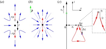
The relevant geometric parameters. Sketch of the flow field around (a) a force-free extended pusher swimmer, the so-called ‘di-stokeslet’, and (b) the corresponding pusher point stresslet. The black dot indicates the centre of the particle; the two open circles mark the positions where the force
 $F\hat{\boldsymbol{p}}$
and counter-force
 $-F\hat{\boldsymbol{p}}$
are applied to the fluid (red arrows);
 $l$
denotes the dipole length; the green arrow shows the orientation
 $\hat{\boldsymbol{p}}$
of both swimmers; and the blue arrows give an impression of the streamlines around the swimmer. For the stresslet, the streamlines originate and terminate in the origin and are straight. The transition from outward to inward flow happens at a fixed angle (
 $\arccos (1/\sqrt{3})$
), as indicated by the blue dotted lines. (c) Two-dimensional representation of the bulk geometry. The trajectory of the swimmer (green circle) is along the
 $z$
-axis from
 $-\infty$
to
 $\infty$
, which the swimmer traverses with speed
 $v_{s}$
. The tracer (blue circle) is advected along the red trajectory – here we have assumed a puller-type swimmer. The initial position of the tracer (black circle) is given by
 $x_{i}\hat{\boldsymbol{x}}$
. The tracer displacement due to advection by the swimmer flow field is measured using
 $\unicode[STIX]{x0394}x$
and
 $\unicode[STIX]{x0394}z$
, which are measured with respect to
 $x_{i}$
and
 $z_{i}$
. The final tracer position, as assumed once the swimmer has completed its trajectory, is given by
 $x_{f}$
and
 $z_{f}$
(see the inset).

We start by considering the effect of swimmer–tracer separation and the difference between the extended ‘di-stokeslet’ and point stresslet descriptions of a microswimmer (see figure 1 a,b) in an infinite (non-periodic) system. Here, we confirm that, for small swimmer–tracer separations, the tracers exhibit non-closed trajectories, leading to deviations from the standard concave triangular trajectories followed by tracers advected in dipolar flow fields (Pushkin et al. Reference Pushkin, Shum and Yeomans2013; Pushkin & Yeomans Reference Pushkin and Yeomans2013). Furthermore, in this regime, we find that the difference between the stresslet and di-stokeslet descriptions becomes appreciable. Next, we extend the Ewald-summation method for stokeslets put forward by Beenakker (Reference Beenakker1986) and detailed in Pozrikidis (Reference Pozrikidis1996) to properly include the effect of PBCs. We show that these significantly impact the trajectories of the tracers, even for small swimmer–tracer separation and relatively large boxes. Finally, we investigate the limit of large simulation boxes and find that unpractically large sizes – from the perspective of simulations – are needed for convergence to the bulk system. Our work therefore raises questions concerning the suitability of common fluid-dynamic solvers to study the bulk behaviour of microswimmers.
2 Theory
The velocity field at a point
 $\boldsymbol{r}$
due to an extended stresslet (‘di-stokeslet’, see figure 1
a) in bulk is given by
 $$\begin{eqnarray}\boldsymbol{u}(\boldsymbol{r})=\frac{F}{8\unicode[STIX]{x03C0}\unicode[STIX]{x1D707}}\left[\unicode[STIX]{x1D64E}\left(\boldsymbol{r}-\frac{l}{2}\hat{\boldsymbol{p}}\right)-\unicode[STIX]{x1D64E}\left(\boldsymbol{r}+\frac{l}{2}\hat{\boldsymbol{p}}\right)\right]\hat{\boldsymbol{p}},\end{eqnarray}$$
where
 $\unicode[STIX]{x1D707}$
is the dynamic viscosity,
 $F$
the force magnitude,
 $l$
the point separation,
 $\hat{\boldsymbol{p}}$
the unit vector indicating the swimmer’s orientation and
 $$\begin{eqnarray}\unicode[STIX]{x1D64E}(\boldsymbol{r})=\frac{1}{r}\left(\unicode[STIX]{x1D644}+\hat{\boldsymbol{r}}\otimes \hat{\boldsymbol{r}}\right)\end{eqnarray}$$
the bulk stokeslet, with
 $\unicode[STIX]{x1D644}$
the identity matrix,
 $r\equiv |\boldsymbol{r}|$
,
 $\hat{\boldsymbol{r}}\equiv \boldsymbol{r}/r$
, and
 $\otimes$
the dyadic product. The corresponding expression for the (point) stresslet is obtained by taking the limit
 $l\rightarrow 0$
(see figure 1
b), yielding a directional derivative and the expression
 $$\begin{eqnarray}\boldsymbol{u}(\boldsymbol{r})=-\frac{\unicode[STIX]{x1D705}}{8\unicode[STIX]{x03C0}\unicode[STIX]{x1D707}}\left[\left(\hat{\boldsymbol{p}}\boldsymbol{\cdot }\unicode[STIX]{x1D735}\right)\unicode[STIX]{x1D64E}(\boldsymbol{r})\right]\hat{\boldsymbol{p}}=\frac{\unicode[STIX]{x1D705}}{8\unicode[STIX]{x03C0}\unicode[STIX]{x1D707}r^{2}}(3(\hat{\boldsymbol{p}}\boldsymbol{\cdot }\hat{\boldsymbol{r}})^{2}-1)\hat{\boldsymbol{r}},\end{eqnarray}$$
with
 $\unicode[STIX]{x1D735}$
the gradient with respect to
 $\boldsymbol{r}$
. In our construction, positive values of the stresslet strength
 $\unicode[STIX]{x1D705}=Fl$
correspond to pusher swimmers and negative values to puller swimmers.
In a system with PBCs, the velocity experienced at
 $\boldsymbol{r}_{\mathbf{0}}$
in the central box due to the array of point forces
 $F\hat{\boldsymbol{p}}$
is formally given by
 $$\begin{eqnarray}\boldsymbol{u}(\boldsymbol{r}_{\mathbf{0}})=\frac{F}{8\unicode[STIX]{x03C0}\unicode[STIX]{x1D707}}\left(\mathop{\sum }_{\boldsymbol{n}}\unicode[STIX]{x1D64E}(\boldsymbol{r}_{\boldsymbol{n}})\right)\hat{\boldsymbol{p}},\end{eqnarray}$$
where
 $\boldsymbol{r}_{\boldsymbol{n}}=\boldsymbol{r}_{\mathbf{0}}-\boldsymbol{X}_{\boldsymbol{n}}$
and
 $\boldsymbol{X}_{\boldsymbol{n}}=n_{0}\boldsymbol{a}+n_{1}\boldsymbol{b}+n_{2}\boldsymbol{c}$
, with
 $\boldsymbol{n}\in \mathbb{Z}^{3}$
and
 $\boldsymbol{a}$
,
 $\boldsymbol{b}$
and
 $\boldsymbol{c}$
the sides of the box. However, the slow
 $1/r$
decay of
 $\unicode[STIX]{x1D64E}$
leads to the sum in (2.4) being conditionally convergent, just as when summing up electrostatic charge and dipole potentials. Thus, the flow field will depend on the order in which the terms are summed. From a physical perspective, however, one usually selects a summation over spherical (or, in the case of a non-cubic box, spheroidal) shells. Furthermore, from a computational viewpoint, the slow convergence of (2.4) makes it necessary to employ more elaborate methods, inspired by the Ewald summation used in electrostatics, to transform the sum into a more rapidly (and absolutely) convergent one.
Here, we will use the formalism put forward by Beenakker (Reference Beenakker1986) and Pozrikidis (Reference Pozrikidis1996), who suggested splitting the stokeslet according to
 $$\begin{eqnarray}\unicode[STIX]{x1D64E}(\boldsymbol{r})=\unicode[STIX]{x1D723}(\boldsymbol{r})+\unicode[STIX]{x1D733}(\boldsymbol{r}),\end{eqnarray}$$
with
 $$\begin{eqnarray}\displaystyle \displaystyle & \unicode[STIX]{x1D723}(\boldsymbol{r})=8\unicode[STIX]{x03C0}\left(\unicode[STIX]{x1D644}\unicode[STIX]{x1D6FB}^{2}-\unicode[STIX]{x1D735}\otimes \unicode[STIX]{x1D735}\right)B(r)\,\text{erfc}(\unicode[STIX]{x1D709}r), & \displaystyle\end{eqnarray}$$
 $$\begin{eqnarray}\displaystyle \displaystyle & \unicode[STIX]{x1D733}(\boldsymbol{r})=8\unicode[STIX]{x03C0}\left(\unicode[STIX]{x1D644}\unicode[STIX]{x1D6FB}^{2}-\unicode[STIX]{x1D735}\otimes \unicode[STIX]{x1D735}\right)B(r)\,\text{erf}(\unicode[STIX]{x1D709}r), & \displaystyle\end{eqnarray}$$
where
 $\unicode[STIX]{x1D6FB}^{2}$
is the Laplacian,
 $B(r)=r/(8\unicode[STIX]{x03C0})$
the fundamental solution of the biharmonic equation,
 $\text{erf}(z)$
the error function,
 $\text{erfc}(z)=1-\text{erf}(z)$
its complement, and
 $\unicode[STIX]{x1D709}\geqslant 0$
is a splitting parameter. Now
 $\unicode[STIX]{x1D723}$
yields a rapidly convergent sum in real space (dominant for
 $\unicode[STIX]{x1D709}\ll 1$
), whereas the long-range part
 $\unicode[STIX]{x1D733}$
(dominant for
 $\unicode[STIX]{x1D709}\gg 1$
) will be handled in Fourier space, where it will also become absolutely convergent. As shown by Pozrikidis (Reference Pozrikidis1996), this splitting yields
 $$\begin{eqnarray}\displaystyle & \displaystyle \unicode[STIX]{x1D723}(\boldsymbol{r})=\frac{1}{r}\left(C(\unicode[STIX]{x1D709}r)\unicode[STIX]{x1D644}+D(\unicode[STIX]{x1D709}r)\hat{\boldsymbol{r}}\otimes \hat{\boldsymbol{r}}\right), & \displaystyle\end{eqnarray}$$
 $$\begin{eqnarray}\displaystyle & \displaystyle C(z)=\text{erfc}(z)+\frac{2z}{\sqrt{\unicode[STIX]{x03C0}}}\left(2z^{2}-3\right)\text{e}^{-z^{2}}, & \displaystyle\end{eqnarray}$$
 $$\begin{eqnarray}\displaystyle & \displaystyle D(z)=\text{erfc}(z)+\frac{2z}{\sqrt{\unicode[STIX]{x03C0}}}\left(1-2z^{2}\right)\text{e}^{-z^{2}} & \displaystyle\end{eqnarray}$$
and
 $$\begin{eqnarray}\check{\unicode[STIX]{x1D733}}(\boldsymbol{k})=\frac{8\unicode[STIX]{x03C0}}{k^{2}}\left(\unicode[STIX]{x1D644}-\hat{\boldsymbol{k}}\otimes \hat{\boldsymbol{k}}\right)\left(1+\frac{\unicode[STIX]{x1D714}^{2}}{4}+\frac{\unicode[STIX]{x1D714}^{4}}{8}\right)\text{e}^{-\unicode[STIX]{x1D714}^{2}/4}\text{e}^{-\text{i}\boldsymbol{k}\boldsymbol{\cdot }\boldsymbol{r}_{\mathbf{0}}},\end{eqnarray}$$
where
 $\check{\unicode[STIX]{x1D733}}$
is the Fourier transform of
 $\unicode[STIX]{x1D733}$
(the ‘check’ symbol is used throughout to denote the transform),
 $\boldsymbol{k}$
is the reciprocal-space wavevector,
 $k\equiv |\boldsymbol{k}|$
,
 $\hat{\boldsymbol{k}}\equiv \boldsymbol{k}/k$
, and
 $\unicode[STIX]{x1D714}\equiv k/\unicode[STIX]{x1D709}$
. The sum in (2.4) is now given by the two absolutely convergent sums,
 $$\begin{eqnarray}\unicode[STIX]{x1D64E}_{PBC}(\boldsymbol{r})\equiv \mathop{\sum }_{\boldsymbol{n}}\unicode[STIX]{x1D64E}(\boldsymbol{r}_{\boldsymbol{n}})=\mathop{\sum }_{\boldsymbol{n}}\unicode[STIX]{x1D723}(\boldsymbol{r}_{\boldsymbol{n}})+\frac{1}{V}\mathop{\sum }_{\boldsymbol{m}\neq \mathbf{0}}\check{\unicode[STIX]{x1D733}}(\boldsymbol{k}_{\boldsymbol{m}}),\end{eqnarray}$$
where
 $V\equiv \boldsymbol{c}\boldsymbol{\cdot }(\boldsymbol{a}\times \boldsymbol{b})$
is the system volume,
 $\boldsymbol{k}_{\boldsymbol{m}}\equiv 2\unicode[STIX]{x03C0}m_{0}(\boldsymbol{b}\times \boldsymbol{c})/V+2\unicode[STIX]{x03C0}m_{1}(\boldsymbol{c}\times \boldsymbol{a})/V+2\unicode[STIX]{x03C0}m_{2}(\boldsymbol{a}\times \boldsymbol{b})/V$
with
 $\boldsymbol{m}\in \mathbb{Z}^{3}$
, and it is assumed that the left-hand side sum is carried out over spherical shells. Note also that the
 $\boldsymbol{k}=\mathbf{0}$
term should be excluded from the right-hand side to eliminate the net force, as discussed in Pozrikidis (Reference Pozrikidis1996).
The velocity field due to a periodic array of stresslets can now be obtained using a similar directional derivative as
 $$\begin{eqnarray}\boldsymbol{u}_{PBC}(\boldsymbol{r})=-\frac{\unicode[STIX]{x1D705}}{8\unicode[STIX]{x03C0}\unicode[STIX]{x1D707}}[(\,\hat{\boldsymbol{p}}\boldsymbol{\cdot }\unicode[STIX]{x1D735})\unicode[STIX]{x1D64E}_{PBC}(\boldsymbol{r})]\,\hat{\boldsymbol{p}}.\end{eqnarray}$$
The real-space part yields
 $$\begin{eqnarray}\left(\hat{\boldsymbol{p}}\boldsymbol{\cdot }\unicode[STIX]{x1D735}\right)\unicode[STIX]{x1D723}(\boldsymbol{r})\hat{\boldsymbol{p}}=\frac{1}{r^{2}}[D(\unicode[STIX]{x1D709}r)\hat{\boldsymbol{r}}-E(\unicode[STIX]{x1D709}r)(\hat{\boldsymbol{r}}\boldsymbol{\cdot }\hat{\boldsymbol{p}})^{2}\hat{\boldsymbol{r}}-F(\unicode[STIX]{x1D709}r)(\hat{\boldsymbol{r}}\boldsymbol{\cdot }\hat{\boldsymbol{p}})\hat{\boldsymbol{p}}],\end{eqnarray}$$
where
 $C(z)$
and
 $D(z)$
are given by (2.9) and (2.10), and we have defined the new auxiliary functions
 $$\begin{eqnarray}\displaystyle & \displaystyle E(z)\equiv 3D(z)-zD^{\prime }(z)=3\,\text{erfc}(z)+\frac{2z}{\sqrt{\unicode[STIX]{x03C0}}}\left(3+2z^{2}-4z^{4}\right)\text{e}^{-z^{2}}, & \displaystyle\end{eqnarray}$$
 $$\begin{eqnarray}\displaystyle & \displaystyle F(z)\equiv C(z)-zC^{\prime }(z)-D(z)=\frac{2z}{\sqrt{\unicode[STIX]{x03C0}}}\left(4z^{4}-8z^{2}\right)\text{e}^{-z^{2}}. & \displaystyle\end{eqnarray}$$
The Fourier-space part is similarly obtained from (2.11) and reads
 $$\begin{eqnarray}(\hat{\boldsymbol{p}}\boldsymbol{\cdot }\unicode[STIX]{x1D735})\check{\unicode[STIX]{x1D733}}(\boldsymbol{k})\hat{\boldsymbol{p}}=-\text{i}(\hat{\boldsymbol{p}}\boldsymbol{\cdot }\hat{\boldsymbol{k}})k\check{\unicode[STIX]{x1D733}}(\boldsymbol{k})\hat{\boldsymbol{p}}.\end{eqnarray}$$
Thus, we may write for the velocity field due to a periodic array of stresslets with dipole strength
 $\unicode[STIX]{x1D705}$
and direction
 $\hat{\boldsymbol{p}}$
,
 $$\begin{eqnarray}\boldsymbol{u}_{PBC}(\boldsymbol{r})=\mathop{\sum }_{\boldsymbol{n}}\boldsymbol{u}_{R}(\boldsymbol{r}_{\boldsymbol{n}})+\frac{1}{V}\mathop{\sum }_{\boldsymbol{m}\neq \mathbf{0}}\boldsymbol{u}_{F}(\boldsymbol{k}_{\boldsymbol{m}}),\end{eqnarray}$$
with
 $$\begin{eqnarray}\boldsymbol{u}_{R}(\boldsymbol{r})\equiv \frac{\unicode[STIX]{x1D705}}{8\unicode[STIX]{x03C0}\unicode[STIX]{x1D707}r^{2}}[E(\unicode[STIX]{x1D709}r)(\hat{\boldsymbol{r}}\boldsymbol{\cdot }\hat{\boldsymbol{p}})^{2}\hat{\boldsymbol{r}}+F(\unicode[STIX]{x1D709}r)(\hat{\boldsymbol{r}}\boldsymbol{\cdot }\hat{\boldsymbol{p}})\hat{\boldsymbol{p}}-D(\unicode[STIX]{x1D709}r)\hat{\boldsymbol{r}}]\end{eqnarray}$$
and
 $$\begin{eqnarray}\boldsymbol{u}_{F}(\boldsymbol{k})\equiv \frac{\text{i}\unicode[STIX]{x1D705}}{\unicode[STIX]{x1D707}k}(\hat{\boldsymbol{p}}\boldsymbol{\cdot }\hat{\boldsymbol{k}})(\unicode[STIX]{x1D644}-\hat{\boldsymbol{k}}\otimes \hat{\boldsymbol{k}})\left(1+\frac{\unicode[STIX]{x1D714}^{2}}{4}+\frac{\unicode[STIX]{x1D714}^{4}}{8}\right)\text{e}^{-\unicode[STIX]{x1D714}^{2}/4}\text{e}^{-\text{i}\boldsymbol{k}\boldsymbol{\cdot }\boldsymbol{r}_{\mathbf{0}}}\hat{\boldsymbol{p}},\end{eqnarray}$$
with
 $D$
,
 $E$
and
 $F$
as defined before. We finally note that these expressions are different from those derived in af Klinteberg & Tornberg (Reference af Klinteberg and Tornberg2014), as those results correspond to a periodic array of singularities that exclude the source term (the second term inside the bracket of (2.3)).
3 Comparison between di-stokeslet and stresslet descriptions
Before assessing the effect of periodic boundaries on tracer trajectories, we will investigate the difference between the extended di-stokeslet and point stresslet descriptions in the near field of an infinite (non-periodic) system. To this end, we follow the strategy of Pushkin et al. (Reference Pushkin, Shum and Yeomans2013) and perform a numerical calculation of the effect of a swimmer passing by a tracer particle, with the swimmer moving from
 $-\infty$
to
 $+\infty$
along the
 $z$
-axis with constant velocity
 $v_{s}$
(see figure 1
c). Over the course of its trajectory, the swimmer interacts with a tracer initially positioned at
 $\boldsymbol{r}_{i}=(x_{i},0,0)$
. Note that, by symmetry, the tracer motion may be restricted to the
 $xz$
-plane. The tracer trajectory is parametrized by
 $\unicode[STIX]{x0394}x=x(t)-x_{i}$
and
 $\unicode[STIX]{x0394}z=z(t)-z_{i}=z(t)$
, and is simply given by the advection it experiences due to the swimmer flow field. These assumptions result in the differential equations
 $$\begin{eqnarray}\displaystyle & \displaystyle \dot{\boldsymbol{r}}_{t}(t)=\boldsymbol{u}(\boldsymbol{r}_{t}(t)-\boldsymbol{r}_{s}(t)), & \displaystyle\end{eqnarray}$$
 $$\begin{eqnarray}\displaystyle & \displaystyle \dot{\boldsymbol{r}}_{s}(t)=v_{s}\hat{\boldsymbol{z}}, & \displaystyle\end{eqnarray}$$
where
 $\boldsymbol{r}_{t}$
and
 $\boldsymbol{r}_{s}$
denote the tracer and swimmer positions, respectively. The fluid velocity
 $\boldsymbol{u}(\boldsymbol{r})$
in bulk is given either by the stresslet expression of (2.3), or its di-stokeslet equivalent, equation (2.1). In the numerics, the swimmer trajectories start at
 $z=-5.0\times 10^{4}$
and end at
 $z=5.0\times 10^{4}$
, using a varying time-step size to ensure an accurate integration when the separation between the swimmer and tracer is small. We further assume
 $\unicode[STIX]{x1D707}=1.0$
in our dimension-free units, and the swim speed is kept constant at
 $v_{s}=1.0\times 10^{-3}$
. We set
 $|\unicode[STIX]{x1D705}|=1.0$
in the stresslet model and
 $l=F=1.0$
in the di-stokeslet model unless otherwise specified. Finally, we denote the final position of the tracer by
 $\boldsymbol{r}_{f}=(x_{f},0,z_{f})$
.
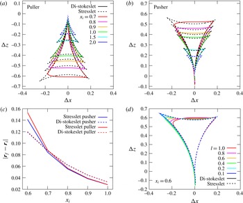
Figure 2(a,b) shows the difference between the di-stokeslet and stresslet descriptions on the advection of tracer particles. For
 $x_{i}>l$
the deviation between the trajectories is minimal. However, for smaller values of the initial separation, there is a clear ‘rounding’ of the di-stokeslet result with respect to that of the stresslet, which is a manifestation of the finite separation between the two force points. Clearly, the effect of the swimmer on the tracer becomes more pronounced as their separation is reduced. Below a certain value of the separation (
 $x_{i}\lesssim 0.5$
for our parameters), the tracer will start interacting with the ‘naked’ singularity at the centre of the swimmer – or the front singularity in the di-stokeslet approximation – leading to numerical divergences in the tracer trajectories. These clearly require regularization, and could be prevented using additional swimmer–tracer interactions accounting for near-field lubrication effects and non-hydrodynamic interaction potentials; this is not considered here.
Near-field trajectories of tracers advected by (a) pusher and (b) puller swimmers in an infinite (bulk) system. The results for the di-stokeslet (
 $l=1$
) are given by the solid curves and for the stresslet by the dashed curves. (c) The net tracer displacement by a stresslet swimmer. The difference between the initial and final positions of the tracer
 $|\boldsymbol{r}_{f}-\boldsymbol{r}_{i}|$
after the swimmer has completed its trajectory is given as a function of the initial tracer position
 $x_{i}$
. The results for pushers are shown in blue and for pullers in red. For both swimmer types the sign of the displacement is the same: negative for the
 $z$
coordinate and positive for the
 $x$
coordinate. (d) Comparison between the tracer trajectories caused by a pusher di-stokeslet (solid curves) and stresslet (dashed curves) in bulk as a function of the di-stokeslet length
 $l$
(keeping
 $\unicode[STIX]{x1D705}=1.0$
constant) for
 $x_{i}=0.6$
.

It is also clear from figure 2(a,b) that the trajectory due to the stresslet swimmer becomes increasingly asymmetric with decreasing
 $x_{i}$
. This can be explained by the tracer being increasingly subjected to the near-field flow of the swimmer. In both the near and far fields, the Darwin drift (Darwin Reference Darwin1953; Pushkin et al.
Reference Pushkin, Shum and Yeomans2013) leads to the tracer trajectories not being closed, yielding finite values of
 $\unicode[STIX]{x0394}x$
and
 $\unicode[STIX]{x0394}z$
after the swimmer has moved along its full trajectory. The effect is illustrated in figure 2(c), where the difference
 $|\boldsymbol{r}_{f}-\boldsymbol{r}_{i}|$
between the initial and final positions of the tracer is given as a function of
 $x_{i}$
. As has been pointed out by Pushkin et al. (Reference Pushkin, Shum and Yeomans2013), this difference will approach zero in the limit where the tracer advection is negligible compared to the swimmer movement, i.e.
 $|\dot{\boldsymbol{r}}_{t}|/|\dot{\boldsymbol{r}}_{s}|\rightarrow 0$
, which corresponds to the limit
 $x_{i}\rightarrow \infty$
. However, for the short swimmer–tracer separations studied in figure 2, this displacement is significantly different from zero. Furthermore, we note that the difference in the net displacement between the stresslet and di-stokeslet descriptions is surprisingly small, even though the overall near-field trajectories of these two objects differ significantly.
Finally, we demonstrate that the di-stokeslet results reduce to those of the point stresslet in the limit
 $l\rightarrow 0$
, as expected. Figure 2(d) shows this effect for
 $x_{i}=0.6$
and various values of
 $l$
in the case of a pusher swimmer. For this small swimmer–tracer separation, a value of
 $l\approx 0.1$
gives reasonable convergence to the stresslet result.
4 The effect of periodicity on tracer trajectories
We now assess the effect of PBCs on the interaction between swimmers and tracers. The geometry in which we perform the calculation is sketched in figure 3(a). Our simulation box is cubic with edge length
 $L$
, centred on the origin. The general numerical procedure is thus the same as that described in § 3, apart from that the swimmer now moves from
 $-L/2$
to
 $L/2$
along the
 $z$
-axis. When integrating (3.1) and (3.2), the fluid flow velocity
 $\boldsymbol{u}(\boldsymbol{r})$
is now given by the PBC stresslet expression of (2.18). We furthermore used the value
 $\unicode[STIX]{x1D709}=\unicode[STIX]{x03C0}^{1/2}/L$
suggested by Beenakker (Reference Beenakker1986) for cubic boxes, and (cubic) real- and Fourier-space cutoffs of
 $|n_{max}|$
,
 $|m_{max}|\leqslant 10$
, which gave convergence to within the numerical rounding error with respect to a cutoff of 9.
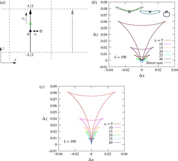
The effect of PBCs on the advection of tracers by microswimmers. (a) Two-dimensional representation of a cubic simulation box with PBCs (dashed black lines). The swimmer (green circle) moves at speed
 $v_{s}$
along the
 $z$
-axis from
 $-L/2$
to
 $L/2$
, with
 $L$
the edge length of the box. The initial position
 $x_{i}\hat{\boldsymbol{x}}$
of the tracer is given by the black circle. One of the periodic duplicates of the system is shown using desaturated colours on the right-hand side. (b) Tracer trajectories in a cubic system with PBCs of edge length
 $L=100$
, for which the initial tracer-swimmer separation
 $x_{i}$
is varied. The three insets show the result for
 $x_{i}=20$
,
 $25$
and
 $40$
(from left to right) magnified by a factor of 2.5 and shifted with respect to the origin for clarity; the shifted origin is indicated using the
 $\times$
symbol. Solid lines show data obtained using the stresslet Ewald expressions, while dashed lines show the corresponding (partially converged) results from a direct summation in spherical shells. (c) Data corresponding to (b), but using the bulk stresslet expression.

Figure 3(b) shows tracer trajectories induced by a periodic array of pusher swimmers with identical properties to those discussed in § 3, for several values of
 $x_{i}$
in a box of length
 $L=100$
. We start by noticing that our Ewald expressions are in accordance with results of an explicit summation of stresslets in spherical shells (dashed lines in figure 3
b). It should be noted, however, that these sums are extremely slowly convergent, and that even for 40 layers of images (corresponding to
 ${\approx}$
85 min of CPU time), the curves are not fully converged to the Ewald results, where the latter require only
 ${\approx}$
10 s of CPU time.
Furthermore, it is clear that, even for relatively small swimmer–tracer separations (
 $x_{i}=5$
), the observed trajectories are significantly perturbed by the use of PBCs. For large separations (
 $x_{i}\geqslant 20$
), the trajectories are qualitatively wrong compared to the bulk results (figure 3
c). Moreover, the PBC results underestimate the maximum value of
 $\unicode[STIX]{x0394}z$
by approximately 25 %, even for the shortest swimmer–tracer separations considered. While the overall PBC trajectories are still approximately closed (i.e.
 $|\boldsymbol{r}_{f}-\boldsymbol{r}_{i}|\approx 0$
, when
 $r_{s}=L/2$
), the observed discrepancy would have a large effect on tracer displacements for tumbling swimmers, where tracer trajectories are not closed.
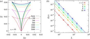
Finite-size scaling for the swimmer–tracer advection and convergence of the flow field. (a) The convergence towards the bulk tracer trajectory (dashed black curve) for a cubic system with PBCs (solid curves) for various values of the box length
 $L$
. The initial separation is kept constant at
 $x_{i}=10$
. (b) The near-field difference
 $E$
(symbols) between the bulk and PBCs flow field as a function of the box length for several distances from the swimmer
 $r$
(see (4.1) for the definition of the error); the dashed lines serve as a guide to the eye for the power-law decay in the error.

As a different manifestation of this effect, we consider the convergence towards the bulk behaviour when increasing the box size while keeping
 $x_{i}$
constant at a value of 10 (figure 4
a). We note that, to obtain a reasonable correspondence with the bulk curve (
 ${\approx}10\,\%$
error), a box length of
 $L=1000$
is needed, corresponding to
 $L/x_{i}=100$
. This is a rather surprising and potentially worrying result, as this is far beyond the system sizes accessible in typical computer simulations. It is furthermore a much more long-ranged effect than what is observed in corresponding simulations of electric dipoles under PBCs, where the periodicity artifacts usually become negligible at length scales
 ${\leqslant}L/2$
(Stenhammar et al.
Reference Stenhammar, Karlström and Linse2011).
To put this result in perspective, we should note that the near-field flow field around the swimmer converges more rapidly, as shown in figure 4(b), which shows the convergence of the fluid flow in PBCs onto that of the bulk stresslet. We computed the relative error
 $E$
in this flow-field reproduction as follows. A stresslet with our standard parameters was placed in the centre of a cubic box with PBCs (or equivalently in bulk). We denote the stresslet-induced flow field in the cubic system with PBCs by
 $\boldsymbol{u}_{L}$
and the bulk flow field by
 $\boldsymbol{u}_{\infty }$
; both are dependent on distance from the swimmer
 $r$
and the polar angle
 $\unicode[STIX]{x1D719}$
. The flow field is cylindrically symmetric and we can therefore ignore the azimuthal angle
 $\unicode[STIX]{x1D703}$
. The error
 $E$
is then given by
 $$\begin{eqnarray}E(r)=\frac{\displaystyle \int _{0}^{\unicode[STIX]{x03C0}}|\boldsymbol{u}_{L}(r,\unicode[STIX]{x1D719})-\boldsymbol{u}_{\infty }(r,\unicode[STIX]{x1D719})|\sin (\unicode[STIX]{x1D719})\,\text{d}\unicode[STIX]{x1D719}}{\displaystyle \int _{0}^{\unicode[STIX]{x03C0}}|\boldsymbol{u}_{\infty }(r,\unicode[STIX]{x1D719})|\sin (\unicode[STIX]{x1D719})\,\text{d}\unicode[STIX]{x1D719}}.\end{eqnarray}$$
This definition has the advantage of being a relative error, weighted with the expected bulk local speed. Convergence to
 $E=0.1$
(
 ${\approx}10\,\%$
error) is reached for all considered distances with
 $L>100$
. The difference between the flow field in the system with PBCs and the bulk flow field decays as
 $L^{-3}$
. That is, the finite-size error scales with the system volume and, as expected, it increases with distance.
By comparison, our tracer trajectories are particularly sensitive to periodicity, since the swimmer traverses the length of the box, thereby always exposing the tracer to the strongly perturbed far field. However, if the physics of the system is partially governed by long-ranged interactions, as is the case for this specific example, then such slow convergence must be accounted for.
5 Conclusions
The results shown here strongly highlight the effect of using periodic boundary conditions (PBCs) in hydrodynamic simulations – such as Stokesian dynamics (Evans et al. Reference Evans, Ishikawa, Yamaguchi and Lauga2011), dissipative particle dynamics (Lugli, Brini & Zerbetto Reference Lugli, Brini and Zerbetto2012) and lattice Boltzmann simulations (Nash, Adhikari & Cates Reference Nash, Adhikari and Cates2008; de Graaf et al. Reference de Graaf, Menke, Mathijssen, Fabritius, Holm and Shendruk2016) – of microswimmers. Specifically, they show that, even on relatively small length scales, the effect of using PBCs rather than a bulk solvent can be dramatic. Tracer advection for these swimmer–tracer separations is expected to contribute strongly to measurable properties such as the mean-square tracer displacement, which one should therefore expect to be significantly underestimated by the use of PBCs. Furthermore, the boundary effects highlighted here will also affect the interaction between swimmers, thus having an impact on the modelling of collective behaviours in biofluids (Krishnamurthy & Subramanian Reference Krishnamurthy and Subramanian2015). On the other hand, our results show that the difference between using extended or point stresslet dipoles is small for other than very short swimmer–tracer separations. In experiments, higher-order singularities, thermal noise, lubrication effects, time-dependent motion (in the case of mechanical swimming) and non-hydrodynamic interactions are, however, likely to dominate at such small separations. In a broader context, this work highlights the importance of boundary and finite-size effects when studying systems with long-range fluid flows.
Acknowledgements
Helpful discussions with M. Cates, L. af Klinteberg, A. Morozov and C. Nardini are kindly acknowledged. J.d.G. thanks the ‘Deutsche Forschungsgemeinschaft’ (DFG) for funding through the SPP 1726 ‘Microswimmers: from single particle motion to collective behavior’ and gratefully acknowledges funding by a Marie Skłodowska-Curie Intra European Fellowship (G.A. no. 654916) within Horizon 2020. J.S. is financed by a Project Grant from the Swedish Research Council (2015-05449).