



1. Introduction
Compared with Galton–Watson processes, many new phenomena arise when considering the branching processes in varying environments (BPVEs hereafter). For example, for the single-type case, Lindvall [Reference Lindvall11] showed that the population size
 $Z_n$
converges almost surely to a random variable
 $Z_\infty$
, which may take a positive value with positive probability, that is, in the words of Kersting [Reference Kersting9], the process may ‘fall asleep’ at some positive state. Fujimagari [Reference Fujimagari6] showed that the tail probability of the extinction time may behave asymptotically like
 $(\log n)^{-1}$
or
 $n^{-\beta}(\beta<1).$
Later, MacPhee and Schuh [Reference MacPhee and Schuh14] discovered that a BPVE may diverge at different exponential rates. Over the past decades, single-type BPVEs have been extensively studied. The criteria for almost sure extinction, asymptotics of the survival probability, distribution of the population size, Yaglom-type limit theorems and many others are known in full generality. For details, we refer the reader to Bhattacharya and Perlman [Reference Bhattacharya and Perlman1], Jagers [Reference Jagers7], Kersting [Reference Kersting9], Chapter 1 of Kersting and Vatutin [Reference Kersting and Vatutin10], and references therein.
There are only a few results about the multitype BPVE and the situation is less satisfying. Jones [Reference Jones8] gave some second moment conditions under which the population size of a multitype BPVE, normalized by its mean, converges almost surely or in
 $L^2$
to a random limit. Further studies on
 $L^p$
and almost sure convergence and the continuity of the limit distribution can be found in Biggins, Cohn, and Nerman [Reference Biggins, Cohn and Nerman2] and Cohn and Wang [Reference Cohn and Wang3]. Recently, under very general assumptions (arbitrary number of types and general offspring distributions), criteria were provided in Dolgopyat et al. [Reference Dolgopyat, Hebbar, Koralov and Perlman4] for almost sure extinction and convergence of the population size (conditioned on survival and normalized by its mean) to an exponential random variable. We notice also that Dolgopyat et al. [Reference Dolgopyat, Hebbar, Koralov and Perlman4] also gave the asymptotics of the survival probabilities. Their proof relies on a generalization of the Perron–Frobenius theorem suitable for studying the products of non-homogeneous non-negative matrices. Let
 $\nu$
be the extinction time and let
 $M_k$
be the mean matrix of offspring distribution of individuals of the
 $(k-1)$
th generation. They showed that
 \begin{align} \dfrac{1}{C}\biggl(\sum_{k=1}^n\lambda_1^{-1}\cdots\lambda_{n}^{-1}\biggr)^{-1}<\mathbb{P}(\nu>n)<C\biggl(\sum_{k=1}^n\lambda_1^{-1}\cdots\lambda_{n}^{-1}\biggr)^{-1}, \end{align}
where
 $0<C<\infty$
is a certain constant, and for
 $k\ge1$
,
 $\lambda_k$
is a number associated with the generalized Perron–Frobenius theorem and depends on the mean matrices
 $M_n$
,
 $n\ge k$
, of the branching process; see [Reference Dolgopyat, Hebbar, Koralov and Perlman4, Proposition 2.1 and Lemma 2.2]. Inspired by (1.1), we may also consider the following questions.
-
(i) The number
 $\lambda_k$
depends on the mean matrices
$M_n$
,
$n\ge k$
, so it is hard to compute explicitly. Therefore, instead of
$\lambda_k$
, we intend to use
$\varrho(M_k)$
, the spectral radius of
$M_k$
, which is directly computable.
-
(ii) Give conditions to ensure a precise asymptotic equivalence of
$\mathbb{P}(\nu>n)$
, i.e. show that for some constant
\begin{equation*} \mathbb{P}(\nu>n)\sim c\biggl(\sum_{k=1}^{n+1} \varrho(M_1)^{-1}\cdots \varrho(M_{k-1})^{-1}\biggr)^{-1} \quad \text{as $ n\rightarrow\infty$,} \end{equation*}
$0<c<\infty.$
-
(iii) Consider further the asymptotics of
$\mathbb{P}(\nu=n).$
We emphasize that even if one knows the asymptotics of
$\mathbb{P}(\nu>n)$
, it is not an easy task to deal with the asymptotics of
$\mathbb{P}(\nu=n).$


Currently, for a multitype BPVE with general offspring distribution, we have no idea how to solve the above questions. In this paper we consider two-type linear-fractional BPVEs with asymptotically constant mean matrices. For the linear-fractional setting, the distribution of the extinction time can be written in terms of the sum of the product
 $\prod_{k=1}^n M_k$
of the mean matrices. But
 $\prod_{k=1}^n M_k$
is hard to estimate. So we construct some new matrix
 $A_k$
which may depend on
 $M_k$
and
 $M_{k+1}.$
The product
 $\prod_{k=1}^nA_k$
is related to the approximants of some continued fractions. Thus, by some delicate analysis of the continued fractions and the product
 $\prod_{k=1}^n A_k$
, we can express the asymptotics of extinction time distribution in terms of the products of the spectral radii of
 $M_k$
, which can be computed explicitly.
We also construct examples for which the mass of the extinction time distribution at n decays with various speeds, for example
 ${c}/{(n^{1/2}\log n)^2}$
,
 ${c}/{n^\beta}$
,
 $\beta>1$
. This observation complements that of Fujimagari [Reference Fujimagari6], who studied the single-type counterpart.
Outline of the paper. In Section 2 we introduce the model and conditions, state the main result and give the main body of its proof. Then, in Section 3, we construct a two-type linear-fractional BPVE whose extinction time exhibits asymptotics very different from those of the homogeneous Galton–Watson process. Sections 4 and 5 are devoted to proving the results required for proving the main theorem.
2. Model and main results
Suppose that
 $M_k$
,
 $k\ge1$
, is a sequence of non-negative
 $2 \times 2$
matrices and
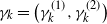 $\gamma_k=\bigl(\gamma_k^{(1)},\gamma_k^{(2)}\bigr)$
,
 $k\ge 1$
, is a sequence of non-negative two-dimensional row vectors. To avoid the degenerate case, we require that, for all
 $ k\ge1$
, all elements of
 $M_kM_{k+1}$
are strictly positive and
 $\gamma_k\ne \mathbf{0}.$
For
 $\mathbf{s}=(s_1,s_2)^t\in [0,1]^2$
and
 $k\ge1$
, let
 \begin{equation*} \mathbf{f}_{k}(\mathbf{s})=\bigl(f_{k}^{(1)}(\mathbf{s}),f_{k}^{(2)}(\mathbf{s})\bigr)^{t}=\mathbf1-\dfrac{M_{k}(\mathbf1-\mathbf{s})}{1+\gamma_{k}(\mathbf1-\mathbf{s})},\end{equation*}
which is known as the probability generating function of a linear-fractional distribution. Here and in what follows,
 $\mathbf{v}^t$
denotes the transpose of a vector
 $\mathbf{v}$
and
 $\mathbf{1}=(\mathbf{e}_1+\mathbf{e}_2)^t=(1,1)^t$
, with
 $\mathbf{e}_1=(1,0),\mathbf{e}_2=(0,1).$
Suppose that
 $Z_n=(Z_{n,1},Z_{n,2})$
,
 $n\ge0$
, is a stochastic process such that
 \begin{equation*} \mathbb{E} \left(\mathbf{s}^{Z_n}\mid Z_0,\ldots,Z_{n-1}\right)= [\mathbf{f}_{n}(\mathbf{s})]^{Z_{n-1}},\quad n\ge1,\end{equation*}
where
 $[\mathbf{f}_{n}(s)]^{Z_{n-1}} \,{:\!=}\, \left[f_n^{(1)}(\mathbf{s})\right]^{Z_{n,1}}\left[f_n^{(2)}(\mathbf{s})\right]^{Z_{n,2}}.$
We call the process
 $Z_n$
,
 $n\ge0$
, a two-type linear-fractional branching process in a varying environment. Matrices
 $M_k$
,
 $k\ge1$
, are usually referred to as the mean matrices of the branching process. Let
 \begin{equation*}\nu=\min\{n \colon Z_{n}=\mathbf{0}\}\end{equation*}
denote the extinction time of
 $\{Z_n\}$
with which we are concerned.
Throughout, we assume
 $b_k,d_k>0$
,
 $a_k,\theta_k\ge0$
,
 $a_k+\theta_k>0$
,
 $k\ge1$
, and for all
 $k\ge1$
we put
 \begin{align} M_k \,{:\!=}\, \begin{pmatrix} a_k &\,\, b_k\\ d_k &\,\, \theta_k \end{pmatrix}\!,\quad \gamma_k \,{:\!=}\, \mathbf{e}_1M_k.\end{align}
We introduce the following conditions on the numbers
 $a_k,b_k,d_k,\theta_k,k\ge1.$
-
(B1) Suppose that
$b,d>0$
,
$ a,\theta\ge0$
are some numbers such that
$a+\theta>0$
,
$ a_k\rightarrow a$
,
$b_k\rightarrow b $
,
$d_k\rightarrow d$
,
$\theta_k\rightarrow\theta$
as
$k\rightarrow\infty$
, and assume further that (2.2)
\begin{align} \sum_{k=2}^\infty|a_k-a_{k-1}|+| b_k- b_{k-1}|+| d_k- d_{k-1}|+|\theta_{k}-\theta_{k-1}|<\infty.\end{align}


Now suppose that condition (B1) holds, and for
 $k\ge1$
set
 \begin{align} A_k \,{:\!=}\, \begin{pmatrix} \tilde a_k &\,\, \tilde b_k \\ \\[-7pt] \,\tilde{\!d}_k &\,\, 0 \\ \end{pmatrix}\quad \text{with }\tilde a_k=a_k+\dfrac{b_k\theta_{k+1}}{ b_{k+1}}, \ \tilde b_k= b_k,\ \tilde d_k=d_k-\dfrac{a_k\theta_k}{b_k}.\end{align}
Letting
 \begin{equation*}\Lambda_k= \begin{pmatrix} 1 &\,\, 0 \\ \\[-7pt] \theta_k/b_k &\,\, 1 \\ \end{pmatrix}\!,\quad k\ge1, \end{equation*}
then for
 $n\ge k\ge1$
we have
 \begin{align} A_k=\Lambda_k^{-1}M_k\Lambda_{k+1}\quad\text{and}\quad \mathbf{e}_1\prod_{i=k}^n M_i\mathbf{1}=\mathbf{e}_1 \prod_{i=k}^n A_i(1,1-\theta_{n+1}/b_{n+1})^t.\end{align}
Remark 2.1. Note that the distribution of
 $\nu$
is determined in terms of
 $M_k$
; see (4.1) and (4.2) below. However, the elements of
 $\prod_{i=k}^n M_i$
are hard to compute and evaluate, whereas those of
 $\prod_{i=k}^n A_i$
are workable because they have some correspondence with continued fractions due to the special structure of the matrices
 $A_i$
,
 $i\ge1.$
Therefore, instead of
 $M_k$
, we will work with
 $A_k$
below.
We need in addition the following conditions, which are mutually exclusive.
-
(B2) a There exists
$k_0>0$
such that and the limit
\begin{equation*}\dfrac{\tilde a_k}{\tilde b_k}=\dfrac{\tilde a_{k+1}}{\tilde b_{k+1}}, \quad \dfrac{\,\tilde{\!d}_k}{\tilde b_k}\ne\dfrac{\,\tilde{\!d}_{k+1}}{\tilde b_{k+1}}\quad \text{for all $ k\ge k_0$} \end{equation*}
exists.
\begin{equation*}\lim_{k\rightarrow\infty}\dfrac{\,\tilde{\!d}_{k+2}/\tilde b_{k+2}-\,\tilde{\!d}_{k+1}/\tilde b_{k+1}}{\,\tilde{\!d}_{k+1}/\tilde b_{k+1}-\,\tilde{\!d}_{k}/\tilde b_{k}}\end{equation*}
-
(B2) b There exists
$k_0>0$
such that and the limit
\begin{equation*} \dfrac{\tilde a_k}{\tilde b_k}\ne\dfrac{\tilde a_{k+1}}{\tilde b_{k+1}}, \quad \dfrac{\,\tilde{\!d}_k}{\tilde b_k}=\dfrac{\,\tilde{\!d}_{k+1}}{\tilde b_{k+1}}\quad \text{for all $ k\ge k_0$} \end{equation*}
exists.
\begin{equation*}\lim_{k\rightarrow\infty}\dfrac{\tilde a_{k+2}/\tilde b_{k+2}-\tilde a_{k+1}/\tilde b_{k+1}}{\tilde a_{k+1}/\tilde b_{k+1}-\tilde a_{k}/\tilde b_{k}}\end{equation*}
-
(B2) c There exists
$k_0>0$
such that and
\begin{equation*} \dfrac{\tilde a_k}{\tilde b_k}\ne\dfrac{\tilde a_{k+1}}{\tilde b_{k+1}}, \quad \dfrac{\,\tilde{\!d}_k}{\tilde b_k}\ne\dfrac{\,\tilde{\!d}_{k+1}}{\tilde b_{k+1}}\quad \text{for all $k\ge k_0$} \end{equation*}
exists as a finite or infinite number. In addition, if
\begin{equation*}\tau \,{:\!=}\, \lim_{k\rightarrow\infty}\dfrac{\,\tilde{\!d}_{k+1}/\tilde b_{k+1}-\,\tilde{\!d}_{k}/\tilde b_k}{\tilde a_{k+1}/\tilde b_{k+1}-\tilde a_{k}/\tilde b_k}\ne \dfrac{-(a+\theta)\pm \sqrt{(a+\theta)^2+4(bd-a\theta)}}{2b} \end{equation*}
$\tau$
is finite, assume further that exists. Otherwise, if
\begin{equation*}\lim_{k\rightarrow\infty}\dfrac{\tilde a_{k+2}/\tilde b_{k+2}-\tilde a_{k+1}/\tilde b_{k+1}}{\tilde a_{k+1}/\tilde b_{k+1}-\tilde a_{k}/\tilde b_{k}}\end{equation*}
$\tau$
is infinite, assume further that exists.
\begin{equation*} \lim_{k\rightarrow\infty}\dfrac{\,\tilde{\!d}_{k+2}/\tilde b_{k+2}-\,\tilde{\!d}_{k+1}/\tilde b_{k+1}}{\,\tilde{\!d}_{k+1}/\tilde b_{k+1}-\,\tilde{\!d}_{k}/\tilde b_{k}} \end{equation*}


Remark 2.2. (i) We remark that (2.2) of condition (B1) is the requirement of [Reference Sun and Wang16, Theorem 1], which we use to prove Theorem 2.1 below. (ii) Conditions (B2)
 $_a$
, (B2)
 $_b$
, and (B2)
 $_c$
look a bit complicated. The lemma below gives an example for which (B1) and one of (B2)
 $_a$
, (B2)
 $_b$
, and (B2)
 $_c$
hold. Further examples can also be found in Section 3.
Lemma 2.1. Suppose that b,
 $d>0$
and a,
 $\theta\ge0$
are numbers which are not all equal, satisfying
 $a+\theta>0$
,
 \begin{equation*} \tau \,{:\!=}\, \dfrac{b(b+d-a-\theta)+2(a\theta-bd)}{b(2b-a-\theta)}\ne \dfrac{-(a+\theta)\pm\sqrt{(a+\theta)^2+4(bd-a\theta)}}{2b} , \end{equation*}
and
 $(b-a)(b-\theta)\ge0.$
Let
 $r_n$
,
 $n\ge 1$
, be strictly positive numbers such that
 $\lim_{n\rightarrow\infty}r_n=0$
and
 $\lim_{n\rightarrow\infty}{r_n-r_{n+1}}/{r_n^{2}}=c$
for some number
 $0<c<\infty.$
Set
 $a_k=a+r_k$
,
 $b_k=b+r_k$
,
 $d_k=d+r_k$
, and
 $\theta_k=\theta+r_k$
,
 $k\ge1.$
Then
 $a_k,b_k,d_k,\theta_k,k\ge1$
satisfy condition (B1)and one of conditions (B2)
 $_{ a}$
, (B2)
 $_{ b}$
, and (B2)
 $_{ c}.$
The proof of Lemma 2.1 is postponed to the Appendix. Note that under condition (B1) we have
 \begin{equation} \lim_{k\rightarrow\infty}M_k=M \,{:\!=}\, \begin{pmatrix} a &\,\, b \\ \\[-7pt] d &\,\, \theta \end{pmatrix}\!,\quad \lim_{k\rightarrow\infty} A_k=A \,{:\!=}\, \begin{pmatrix} a+\theta &\,\, b \\ \\[-7pt] d-a\theta/b &\,\, 0 \end{pmatrix}\!,\end{equation}
whose eigenvalues are
 \begin{align*} \varrho(M)&=\varrho(A)=\dfrac{a+\theta+\sqrt{(a+\theta)^2+4(bd- a\theta)}}{2},\\[3pt] \varrho_1(M)&=\varrho_1(A)=\dfrac{a+\theta-\sqrt{(a+\theta)^2+4(bd-a\theta)}}{2}.\end{align*}
Clearly we have
 $|\varrho_1(A)|<\varrho(A).$
In the literature, the top eigenvalue
 $\varrho(A)$
is usually referred to as the spectral radius of A. In what follows, we always let
 $\varrho(A)$
denote the spectral radius of a matrix A.
In the rest of the paper,
 $f(n)\sim g(n)$
means
 $\lim_{n\rightarrow\infty}f(n)/g(n)=1$
,
 $f(n)={\mathrm{o}}(g(n))$
means
 $\lim_{n\rightarrow\infty}f(n)/g(n)=0$
, and unless otherwise specified,
 $0<c<\infty$
is some constant, which may change from line to line. We always assume that the empty product is the identity and the empty sum equals
 $0.$
Now we are ready to state the main result.
Theorem 2.1. Suppose that condition (B1)and one of conditions (B2)
 $_{ a}$
, (B2)
 $_{ b}$
, and (B2)
 $_{ c}$
hold. Assume further that
 $|\varrho_1(M)|<1$
and
 $\,\tilde{\!d}_k\ge\varepsilon$
,
 $k\ge1$
, for some
 $\varepsilon>0.$
Then
 \begin{align} &\mathbb{P}(\nu>n \mid Z_0=\mathbf{e}_1)\sim \dfrac{c}{\sum_{k=1}^{n+1} \varrho(M_1)^{-1}\cdots \varrho(M_{k-1})^{-1}}\quad as\,\,\, n\rightarrow\infty. \end{align}
If we assume
 $\theta\ne b+1$
in addition, then as
 $n\rightarrow\infty$
,
 \begin{align} &\mathbb{P}(\nu=n \mid Z_0=\mathbf{e}_1)\sim\dfrac{c\varrho(M_1)^{-1}\cdots \varrho(M_n)^{-1}}{\big(\sum_{k=1}^{n+1} \varrho(M_1)^{-1}\cdots \varrho(M_{k-1})^{-1}\big)^2}. \end{align}
Otherwise, if we suppose
 $\theta= b+1$
further, then as
 $n\rightarrow\infty$
,
 \begin{align} &\mathbb{P}(\nu=n \mid Z_0=\mathbf{e}_1)={\textrm{o}} \Bigg(\dfrac{\varrho(M_1)^{-1}\cdots \varrho(M_n)^{-1}}{\big(\sum_{k=1}^{n+1} \varrho(M_1)^{-1}\cdots \varrho(M_{k-1})^{-1}\big)^2}\Bigg). \end{align}
Remark 2.3. (a) The right-hand sides of (2.6) and (2.7) are computable and easy to estimate. In Section 3, we give an example for which the conditions of Theorem 2.1 hold and
 $\mathbb{P}(\nu=$
 $n \mid Z_0=\mathbf{e}_1)$
decays with various speeds, for example
 ${c}/{(n^{1/2}\log n)^2}$
,
 ${c}/{n^\beta}$
,
 $\beta>1$
as
 $n\rightarrow\infty$
, which are very different from those of homogeneous Galton–Watson processes. (b) The condition
 $\,\tilde{\!d}_k=d_k-a_k\theta_k/b_k\ge \varepsilon$
,
 $ k\ge1 $
, for some
 $\varepsilon>0$
(implying
 $bd>a\theta$
) is a technical one, which ensures that
 $A_k$
,
 $k\ge1$
, are non-negative matrices. In a subsequent work [Reference Wang17], we show that it suffices to assume
 $bd\ne a\theta.$
If
 $bd=a\theta$
, that is, the matrix M is of rank one, our method does not work.
Proof. For convenience of the reader, we give here the main body of the proof of Theorem 2.1. But the proofs of the four lemmas below, especially those of Lemmas 2.3 and 2.4, are the main challenges of this paper and will be postponed to Sections 4 and 5 below.
To begin with, write
 $\tilde p_n\equiv \mathbb{P}(\nu=n \mid Z_0=\mathbf{e}_1)$
and
 $ \tilde\eta_n\equiv \mathbb{P}(\nu>n \mid Z_0=\mathbf{e}_1).$
The lemma below explicitly gives the formulae of
 $\tilde p_n$
and
 $\tilde \eta_n.$
Lemma 2.2. For
 $n\ge1$
, we have
 \begin{align} \tilde\eta_n&=\dfrac{\mathbf{e}_1\prod_{k=1}^{n}A_k(1,\lambda_{n+1})^t}{\sum_{k=1}^{n+1}\mathbf{e}_1\prod_{i=k}^{n}A_i(1,\lambda_{n+1})^t},\end{align}
 \begin{align} \tilde p_n&=\dfrac{1}{\sum_{k=1}^{n+1}\mathbf{e}_1\prod_{i=k}^{n}A_i(1,\lambda_{n+1})^t}\dfrac{\mathbf{e}_1\prod_{k=1}^{n-1}A_{k}\mathbf{e}_1^t}{\sum_{k=1}^{n}\mathbf{e}_1\prod_{i=k}^{n-1}A_i(1,\lambda_{n})^t}G_{n-1}, \end{align}
where
 $\lambda_n \,{:\!=}\, 1-{\theta_n}/{b_n}$
and
 \begin{align} G_{n-1}& \equiv \dfrac{\mathbf{e}_1\prod_{k=1}^{n-1}A_k(1,\lambda_{n})^t\sum_{k=1}^{n+1}\mathbf{e}_1\prod_{i=k}^{n}A_i(1,\lambda_{n+1})^t}{\mathbf{e}_1\prod_{k=1}^{n-1}A_{k}\mathbf{e}_1^t}\notag\\[3pt] &\quad\, -\dfrac{\mathbf{e}_1\prod_{k=1}^{n}A_{k}(1,\lambda_{n+1})^t\sum_{k=1}^{n}\mathbf{e}_1\prod_{i=k}^{n-1}A_i(1,\lambda_{n})^t}{\mathbf{e}_1\prod_{k=1}^{n-1}A_{k}\mathbf{e}_1^t}. \end{align}
 $G_n$
defined in (2.11) looks very complicated. Its convergence in the next lemma plays a key role.
Lemma 2.3. Suppose that condition (B1)holds,
 $|\varrho_1(A)|<1$
and
 $\,\tilde{\!d}_k\ge\varepsilon$
,
 $ k\ge1$
, for some
 $\varepsilon>0.$
Then
 \begin{equation*} \lim_{n\rightarrow\infty}G_n=G\end{equation*}
exists. Moreover, we have
 $0<G<\infty$
if
 $\theta\ne b+1$
and
 $G=0$
if
 $\theta=b+1.$
For
 $n\ge1$
, let
 \begin{equation*} S_n \,{:\!=}\, \dfrac{\sum_{k=1}^{n+1}\varrho(A_1)^{-1}\cdots\varrho(A_{k-1})^{-1}}{\varrho(A_1)^{-1}\cdots\varrho(A_n)^{-1}}. \end{equation*}
Lemma 2.4. Under the conditions of Theorem 2.1, we have
 \begin{align} \mathbf{e}_1\prod_{i=1}^{n}A_n\mathbf{e}_1^t\sim c\varrho(A_1)\cdots\varrho(A_{n})\quad {as\,\, n\rightarrow\infty,} \end{align}
and for some numbers
 $0<\phi_1$
,
 $\phi_2<\infty$
,
 \begin{align} \lim_{n\rightarrow\infty}&\dfrac{\sum_{k=1}^{n+1}\mathbf{e}_1\prod_{i=k}^{n}A_i(1,\lambda_{n+1})^t}{S_n}=\phi_1 \quad {and}\quad \lim_{n\rightarrow\infty}\dfrac{S_{n-1}}{S_n}=\phi_2. \end{align}
We only give here the proof of (2.7), since (2.6) and (2.8) can be proved similarly. Now suppose that
 $\theta\ne b+1.$
Noticing that from (2.5) we get
 $\lim_{n\rightarrow\infty} \varrho(A_n)=\varrho(A)>0$
, it thus follows immediately from the above three lemmas that
 \begin{align} &\tilde p_n\sim\dfrac{c\varrho(A_1)^{-1}\cdots \varrho(A_n)^{-1}}{\big(\sum_{k=1}^{n+1} \varrho(A_1)^{-1}\cdots \varrho(A_{k-1})^{-1}\big)^2}. \end{align}
The lemma below allows us to go from the matrices
 $A_k$
back to
 $M_k$
,
 $k\ge1.$
Lemma 2.5. Suppose that condition (B1)is satisfied and
 $\,\tilde{\!d}_k\ge \varepsilon$
,
 $k\ge1$
, for some
 $\varepsilon>0.$
Then, as
 $n\rightarrow\infty$
,
 \begin{equation*}\dfrac{\varrho(A_1)^{-1}\cdots \varrho(A_n)^{-1}}{\big(\sum_{k=1}^{n+1} \varrho(A_1)^{-1}\cdots \varrho(A_{k-1})^{-1}\big)^2}\sim \dfrac{c\varrho(M_1)^{-1}\cdots \varrho(M_n)^{-1}}{\big(\sum_{k=1}^{n+1} \varrho(M_1)^{-1}\cdots \varrho(M_{k-1})^{-1}\big)^2}.\end{equation*}
As a result, taking (2.14) and Lemma 2.5 together, we get (2.7).
Lemma 2.4 is a consequence of Proposition 2.1 below, which may be of independent interest in the theory of products of positive matrices. Let
 \begin{equation*} B_k= \begin{pmatrix} a_k &\,\, b_k \\ \\[-7pt] d_k &\,\, 0 \\ \end{pmatrix}\!,\quad k\ge1. \end{equation*}
Proposition 2.1. Suppose that
 $a_k,b_k,d_k,\theta_k$
,
 $k\ge1$
satisfy condition (B1)and one of conditions (B2)
 $_a$
, (B2)
 $_b$
, and (B2)
 $_c$
, with
 $\theta_k\equiv 0$
,
 $k\ge1$
, and the number
 $a>0.$
Then, for all
 $ i,j\in \{1,2\}$
, we have
 \begin{align} \mathbf{e}_iB_1\cdots B_n\mathbf{e}_j^t\sim c\varrho(B_1)\cdots\varrho(B_n)\quad {as\,\, n\rightarrow\infty.} \end{align}
Furthermore, writing
 \begin{equation*}\tilde S_n \,{:\!=}\, \dfrac{\sum_{k=1}^{n+1}\varrho(B_1)^{-1}\cdots\varrho(B_{k-1})^{-1}}{\varrho(B_1)^{-1}\cdots\varrho(B_n)^{-1}},\quad Y_n \,{:\!=}\, \dfrac{\sum_{k=1}^{n+1}\mathbf{e}_1B_k\cdots B_n\mathbf{e}_1^t}{\tilde S_n},\quad n\ge0,\end{equation*}
then for some number
 $\psi>0$
we have
 \begin{align} \lim_{n\rightarrow\infty}Y_n=\psi. \end{align}
Remark 2.4. (i) The limit number
 $\psi$
can be deduced from (5.44) and (5.45) below. (ii) Even though we have (2.15) in hand, it is still hard to evaluate
 $\sum_{k=1}^{n+1}\mathbf{e}_1B_k\cdots B_n\mathbf{e}_1^t$
since every summand there depends on n. But by (2.16),
 $\sum_{k=1}^{n+1}\mathbf{e}_1B_k\cdots B_n\mathbf{e}_1^t $
is asymptotically the same as
 $\tilde S_n$
, which is computable.
3. Examples
For
 $n\ge1$
, let
 $q_{n,1}\ge0$
,
 $q_{n,2}>0$
,
 $p_n>0$
be numbers such that
 $q_{n,1}+q_{n,2}+p_n=1.$
Suppose that
 $Z_n$
,
 $n\ge0$
, is a two-type branching process with
 $Z_0=\mathbf{e}_1$
and offspring distributions
 \begin{align} \mathbb{P}(Z_{n}=(i,j)\mid Z_{n-1}=\mathbf{e}_{1})&=\dfrac{(i+j)!}{i!j!}q_{n,1}^{i}q_{n,2}^{j}p_{n},\end{align}
 \begin{align} \nonumber\\[-36pt] \mathbb{P}(Z_{n}=(1+i,j)\mid Z_{n-1}=\mathbf{e}_{2})&=\dfrac{(i+j)!}{i!j!}q_{n,1}^{i}q_{n,2}^{j}p_{n},\end{align}
where
 $i\ge0$
,
 $j\ge 0$
,
 $n\ge1.$
Some computation yields that the mean matrix
 \begin{equation*}M_n \,{:\!=}\, \begin{pmatrix} a_n &\,\, b_n \\ \\[-7pt] 1+a_n &\,\, b_n \end{pmatrix}\quad\text{with } a_n \,{:\!=}\, \dfrac{q_{n,1}}{p_{n}},\ b_n \,{:\!=}\, \dfrac{q_{n,2}}{p_{n}},\quad n\ge1.\end{equation*}
Also, it follows from (3.1) and (3.2) that
 \begin{equation*}F_{n}(\mathbf{s}) \,{:\!=}\, \mathbb{E}\left(s_{1}^{Z_{n,1}}s_{2}^{Z_{n,2}}\mid Z_0=\mathbf{e}_1\right)=1-\dfrac{\mathbf{e}_{1}\prod_{j=1}^{n}M_{j}(\mathbf{1}-\mathbf{s})}{1+\sum_{k=1}^{n}\mathbf{e}_{1}\prod_{i=k}^{n}M_{i}(\mathbf1-\mathbf{s})} ,\end{equation*}
which leads to
 \begin{align} \eta_n &\,{:\!=}\, \mathbb{P}(\nu=n \mid Z_0=\mathbf{e}_1)=F_n(\mathbf{0})-F_{n-1}(\mathbf{0})\notag\\[3pt] &=\dfrac{\mathbf{e}_{1}\prod_{j=1}^{n-1} M_{j}\mathbf1}{\sum_{k=1}^{n}\mathbf{e}_{1}\prod_{i=k}^{n-1}M_{i}\mathbf1}-\dfrac{\mathbf{e}_{1}\prod_{j=1}^{n}M_{j}\mathbf{1}}{\sum_{k=1}^{n+1}\mathbf{e}_{1}\prod_{i=k}^{n}M_{i}\mathbf1}.\end{align}
First we see what happens to the homogeneous case, that is,
 \begin{align} q_{n,1}\equiv q_1,\ q_{n,2}\equiv q_2,\ p_n\equiv p \quad \text{so that } M_n\equiv M \,{:\!=}\, \begin{pmatrix} q_1/p &\,\, q_2/p \\ \\[-7pt] 1+q_1/p &\,\, q_2/p \end{pmatrix}\!,\quad n\ge1,\notag\end{align}
where we assume
 $p>0$
,
 $q_1\ge0$
,
 $q_2>0$
, and
 $p+q_1+q_2=1$
, which ensure that
 $Z_n$
,
 $n\ge0$
, is truly a two-type branching process. Clearly the spectral radius of M is
 \begin{equation*}\varrho(M)=\dfrac{q_1+q_2+\sqrt{(q_1+q_2)^2+4pq_2}}{2p}.\end{equation*}
By some easy computation, from (3.3), we get that as
 $n\rightarrow\infty$
,
 \begin{equation*} \eta_n=\dfrac{\mathbf{e}_1M^{n-1}\mathbf{1}}{\sum_{k=0}^{n-1}\mathbf{e}_1M^k\mathbf{1}}-\dfrac{\mathbf{e}_1M^n\mathbf{1}}{\sum_{k=0}^n\mathbf{e}_1M^k\mathbf{1}} \sim \begin{cases} c\varrho(M)^n &\text{if $\varrho(M)<1$,} \\[3pt] c\varrho(M)^{-n} &\text{if $\varrho(M)>1$,} \\[3pt] n^{-2} &\text{if $\varrho(M)=1$.} \end{cases}\end{equation*}
We thus come to the conclusion that for a homogeneous Galton–Watson process,
 $\mathbb{P}(\nu=n \mid$
 $Z_0=\mathbf{e}_1)$
decays either exponentially (supercritical and subcritical cases) or polynomially (critical case).
Next we consider BPVEs by adding some perturbations on a critical homogeneous Galton–Watson process, which may exhibit very different asymptotics. For
 $K= 1,2,\ldots $
and
 $B\in \mathbb R$
, set
 \begin{align*} &\Lambda(1,i,B)=\dfrac{B}{i},\\ &\Lambda(2,i,B)=\dfrac{1}{i}+\dfrac{B}{i\log i}, \ldots,\\ &\Lambda(K,i,B)=\dfrac{1}{i}+\dfrac{1}{i\log i}+\cdots +\dfrac{1}{i\log i\cdots\log_{K-2}i}+\dfrac{B}{i\log i\cdots\log_{K-1}i}, \end{align*}
where
 $\log_0 i=i$
, and for
 $k\ge1$
,
 $\log_{k}i=\log \log_{k-1} i.$
Now fix K and B, set
 \begin{equation*} i_0 \,{:\!=}\, \min \{i\,{:}\log_{K-1}i>0, {|\Lambda(K,i,B)|}< 1 \}, \end{equation*}
and let
 \begin{equation*} r_i \,{:\!=}\, \begin{cases} \dfrac{\Lambda(K,i,B)}{3} & i\ge i_0, \\ r_{i_0} & i< i_0, \end{cases} \end{equation*}
which serve as perturbations. To avoid tedious computation, we assume
 $q_{n,1}\equiv 0$
, for all
 $ n\ge1$
, and write
 $q_{n,2}$
simply as
 $q_n$
for
 $n\ge1$
so that (3.1) and (3.2) reduce to
 \begin{align} &\mathbb{P}(Z_{n}=(0,j)\mid Z_{n-1}=\mathbf{e}_{1})=q_{n}^{j}p_{n},\end{align}
 \begin{align}&\mathbb{P}(Z_{n}=(1,j)\mid Z_{n-1}=\mathbf{e}_{2})=q_{n}^{j}p_{n},\quad j\ge0,\ n\ge1.\end{align}
Theorem 3.1. Suppose that
 $Z_n$
,
 $n\ge0$
, is a two-type branching process whose offspring distribution satisfies (3.4)and (3.5). Fix
 $K=1,2,3,\ldots $
and
 $B\in \mathbb R.$
-
(i) If
$p_i=\frac{2}{3}+r_i$
,
$q_i=\frac{1}{3}-r_i$
,
$i\ge 1$
, then, as
$n\rightarrow\infty$
,
\begin{equation*} \mathbb{P}(\nu=n\mid Z_0=\mathbf{e}_1)\sim \begin{cases} \dfrac{c }{n\log n\cdots \log_{K-2}n\log_{K-1} n(\log_K n)^2} & {if\ B=1,} \\ \\[-7pt] \dfrac{c}{n\log n\cdots \log_{K-2}n(\log_{K-1} n)^B} & {if\ B>1,} \\\\[-7pt] \dfrac{c}{n\log n\cdots \log_{K-2}n(\log_{K-1} n)^{2-B}} & {if\ B<1.} \end{cases}\end{equation*}
-
(ii) If
$ p_i=\frac{2}{3}-r_i$
,
$q_i=\frac{1}{3}+r_i$
,
$i\ge 1$
, then, as
$n\rightarrow\infty$
,
\begin{equation*} \mathbb{P}(\nu=n\mid Z_0=\mathbf{e}_1)\sim \begin{cases}\dfrac{c}{n^{B+2}} &{if\ K=1,B>-1,}\\ \\[-7pt] \dfrac{c}{n(\log n)^2} & {if\ K=1, B=-1,}\\ \\[-7pt] cn^B & {if\ K=1,B<-1,}\\ \\[-7pt] \dfrac{c}{n^3\log n \ldots \log_{K-2}n (\log_{K-1} n)^B} &{if\ K>1.}\end{cases}\end{equation*}


Remark 3.1. As seen above, for a two-type homogeneous Galton–Watson branching process,
 $\mathbb{P}(\nu=n\mid Z_0=\mathbf{e}_1)$
decays either exponentially or polynomially with speed
 $n^{-2}$
. But for two-type BPVEs,
 $\mathbb{P}(\nu=n\mid Z_0=\mathbf{e}_1)$
may decay with many different speeds such as
 ${c}/{(n^{1/2}\log n)^2}$
,
 $cn^{-B}$
,
 $B>1$
as
 $n\rightarrow\infty.$
Proof. Write
 $b_k=q_k/p_k$
,
 $k\ge1.$
Then
 \begin{equation*} M_k= \begin{pmatrix} 0 &\,\, b_k \\ \\[-7pt] 1 &\,\, b_k \\ \end{pmatrix} \rightarrow M= \begin{pmatrix} 0 &\,\, 1/2 \\ \\[-7pt] 1 &\,\, 1/2 \\ \end{pmatrix}\quad\text{as $k\rightarrow\infty.$} \end{equation*}
Comparing
 $M_k$
with the one in (2.1), we find that
 $a_k\equiv0$
,
 $\theta_k=b_k$
,
 $d_k\equiv 1$
,
 $k\ge1$
, and
 $\varrho(M)=1$
,
 $\varrho_1(M)=-\frac12.$
By definition, we know that
 $\tilde a_k=b_k$
,
 $\tilde b_k=b_k$
,
 $\,\tilde{\!d}_k=d_k\equiv 1.$
Thus
 \begin{equation*} A_k= \begin{pmatrix} b_k &\,\, b_k \\ \\[-7pt] 1 &\,\, 0 \\ \end{pmatrix}\!, \end{equation*}
and it is easily seen that
 $\varrho(A_k)\equiv\varrho(M_k)$
,
 $k\ge1.$
Moreover, we have the following lemma.
Lemma 3.1.
-
(i) We have
and thus
\begin{equation*} \lim\limits_{n\rightarrow\infty}\dfrac{r_n-r_{n+1}}{n^2}=1/3 \end{equation*}
whenever
\begin{equation*} \sum_{k=1}^\infty|b_{k+1}-b_k|<\infty, \end{equation*}
$p_i=2/3\pm r_i$
,
$i\ge 1.$
-
(ii) We have
and
\begin{equation*} \dfrac{1}{b_k}\neq\dfrac{1}{b_{k+1}}\quad{for\, all\, k\ge i_0} \end{equation*}
for any
\begin{equation*} \dfrac{b_{k+1}-b_k}{b_{k+2}-b_{k+1}}\rightarrow1\quad{as\, n\rightarrow\infty} \end{equation*}
$p_i=2/3+r_i$
or
$p_i=2/3-r_i$
,
$i\ge 1.$


For the proof of the lemma we refer the reader to [Reference Sun and Wang16, Lemma 7]. It follows immediately from Lemma 3.1 that conditions (B1) and (B2)
 $_{a}$
are fulfilled. Therefore all conditions of Theorem 2.1 are satisfied. Consequently, applying Theorem 2.1, we conclude that
 \begin{align} \mathbb{P}(\nu=n|Z_0=\mathbf{e}_1)\sim \dfrac{c\varrho(M_1)^{-1}\cdots \varrho(M_n)^{-1}}{\big(\sum_{k=1}^{n+1} \varrho(M_1)^{-1}\cdots \varrho(M_{k-1})^{-1}\big)^2}\quad \text{as $ n\rightarrow\infty$.} \end{align}
Note that
 \begin{equation*}\varrho(M_k)=\Bigl(b_k+\sqrt{b_k^2+4b_k}\Bigr)/2.\end{equation*}
If
 $p_i=\frac{2}{3}\pm r_i$
,
 $i\ge 1$
, then by Taylor expansion of
 $\varrho(M_k)$
at 0 we get
 \begin{equation*}\varrho(M_k)=1\mp 3r_k+{\mathrm{O}} (r_k^2)\quad \text{as $k\rightarrow\infty$.}\end{equation*}
Applying [Reference Sun and Wang16, Proposition 2], we get
 \begin{align} \varrho(M_1)\cdots\varrho(M_n)\sim c \left(n\log n\cdots \log_{K-2}n\left(\log_{K-1} n\right)^B\right)^{\mp 1}.\end{align}
With (3.6) and (3.7) in hand, the proof of Theorem 3.1 is almost identical to that of [Reference Sun and Wang15, Theorem 1]. We do not repeat it here.
4. Proofs of the auxiliary lemmas
The main task of this section is to finish the proofs of the auxiliary lemmas that are required when proving Theorem 2.1. The proof of Lemma 2.4 is based on Proposition 2.1, whose proof is very long and will be postponed to Section 5.
4.1. Proof of Lemma 2.2
Proof. For
 $n\ge 0$
and
 $\mathbf{s}=(s_1,s_2)^t\in [0,1]^2$
, let
 \begin{equation*}F_n^{(i)}(\mathbf{s})\equiv \mathbb{E}\left(\mathbf{s}^{Z_n}\mid Z_0=\mathbf{e}_i\right) \,{:\!=}\, \mathbb{E}\bigl( s_1^{Z_{n,1}}s_2^{Z_{n,2}}\mid Z_0=\mathbf{e}_i\bigr),\quad i=1,2\end{equation*}
and set
 \begin{equation*} \mathbf{F}_n(\mathbf{s})=\left(F_n^{(1)}(\mathbf{s}),\, F_n^{(2)}(\mathbf{s})\right)^t.\end{equation*}
It follows by induction (see [Reference Dyakonova5, Lemma 1]) that for
 $n\ge0$
,
 \begin{equation*} \mathbf{F}_{n}(\mathbf{s})=\mathbf{f}_{1}(\mathbf{f}_{2}(\cdots\mathbf{f}_{n}(\mathbf{s})\cdots)) =\mathbf1-\dfrac{\prod_{k=1}^{n}M_{k}(\mathbf{1}-\mathbf{s})}{1+\sum_{k=1}^{n}\gamma_k\prod_{i=k+1}^{n}M_{i}(\mathbf1-\mathbf{s})},\end{equation*}
which leads to
 \begin{equation*} \mathbf{F}_{n}(\mathbf{0})=\mathbf{1}- \dfrac{\prod_{k=1}^{n}M_{k}\mathbf{1}}{1+\sum_{k=1}^{n}\gamma_k\prod_{i=k+1}^{n}M_{i}\mathbf1}.\end{equation*}
Note that for
 $n\ge1$
and
 $i=1,2$
,
 \begin{align} \mathbb{P}(\nu>n\mid Z_0=\mathbf{e}_i)&=1-F_n^{(i)}(\mathbf{0})=\dfrac{\mathbf{e}_i\prod_{k=1}^{n}M_{k}\mathbf{1}}{\sum_{k=1}^{n+1}\gamma_k\prod_{i=k+1}^{n}M_{i}\mathbf1},\end{align}
and consequently
 \begin{align} \mathbb{P}(&\nu=n\mid Z_0=\mathbf{e}_i)=\dfrac{\mathbf{e}_i\prod_{k=1}^{n-1}M_{k}\mathbf{1}}{\sum_{k=1}^{n}\gamma_k\prod_{i=k+1}^{n-1}M_{i}\mathbf1}-\dfrac{\mathbf{e}_i\prod_{k=1}^{n}M_{k}\mathbf{1}}{\sum_{k=1}^{n+1}\gamma_k\prod_{i=k+1}^{n}M_{i}\mathbf1}.\end{align}
With matrices
 $A_i$
,
 $i\ge1$
being those defined in (2.3), using (2.1) and (2.4), we have from (4.1) and (4.2) that (2.9) and (2.10) hold. Thus Lemma 2.2 is proved.
4.2. Proof of Lemma 2.3
Proof. Due to the complicated formula of
 $G_n$
, the proof will be a long journey. So we divide the proof into several steps. Keep in mind that
 $\lambda_n \,{:\!=}\, 1-\theta_n/b_n\rightarrow 1-\theta/b$
as
 $n\rightarrow\infty.$
Step 1: We show that
 $\lim_{n\rightarrow\infty}G_n=G$
for some number
 $0\le G<\infty.$
For this purpose, set
 \begin{equation*} f_n\equiv \dfrac{\mathbf{e}_1\prod_{k=1}^{n}A_{k}\mathbf{e}_2^t}{\mathbf{e}_1\prod_{k=1}^{n}A_{k}\mathbf{e}_1^t} \quad\text{and}\quad H_n\equiv\sum_{k=1}^{n}\mathbf{e}_1\prod_{i=k}^{n}A_{i}(f_n\mathbf{e}_1^t-\mathbf{e}_2^t),\quad n\ge1.\end{equation*}
Then, by some subtle computation, we get
 \begin{align} G_{n-1}& =1 +(\tilde b_n\lambda_n\lambda_{n+1} +\tilde a_n\lambda_{n}-\,\tilde{\!d}_n)H_{n-1} +(\tilde b_n\lambda_n\lambda_{n+1} +\tilde a_n\lambda_{n}-\,\tilde{\!d}_n+\lambda_{n})f_{n-1}.\end{align}
The next lemma, whose proof is postponed to the end of this subsection, confirms the convergence of
 $f_n$
and
 $H_n$
as
 $n\rightarrow\infty.$
Lemma 4.1. We have
 \begin{align} H_n=\sum_{k=1}^{n-1}(\!-\!1)^{n-k}f_k\,\tilde{\!d}_{k+1}f_{k+1}\cdots \,\tilde{\!d}_nf_n,\quad n\ge1.\notag \end{align}
Furthermore, if condition (B1)holds,
 $|\varrho_1(A)|<1$
and
 $\,\tilde{\!d}_k\ge \varepsilon$
,
 $ k \ge1$
, for some
 $\varepsilon>0$
, then
 \begin{equation*}\lim_{n\rightarrow\infty}f_n=-\dfrac{b\varrho_1(A)}{bd- a\theta}\quad{and}\quad \lim_{n\rightarrow\infty}H_n=-\dfrac{b}{bd- a\theta}\dfrac{\varrho_1(A)^2}{1-\varrho_1(A)}.\end{equation*}
Applying Lemma 4.1, from (4.3) we get
 \begin{equation*} \lim_{n\rightarrow\infty}G_n=G \,{:\!=}\, \dfrac{(b-\theta)\varrho_1(A)^2-(b-\theta)(a+b+1)\varrho_1(A)+bd-a\theta }{(bd-a\theta)(1-\varrho_1(A))}. \end{equation*}
Step 2: Show that
 $0<G<\infty$
if
 $\theta\ne b+1$
and
 $G=0$
if
 $\theta=b+1.$
To begin with, we prove that G is non-negative. Indeed, in view of (2.10), since
 \begin{equation*}\sum_{k=1}^{n}\mathbf{e}_1\prod_{i=k}^{n-1}A_i(1,\lambda_{n})^t=\sum_{k=1}^{n}\mathbf{e}_1\prod_{i=k}^{n-1}M_{i}\mathbf1>0\end{equation*}
and
 \begin{equation*}\mathbf{e}_1\prod_{k=1}^{n-1}A_{k}\mathbf{e}_1^t=\mathbf{e}_1\prod_{k=1}^{n-1}M_{k}\mathbf (1,\theta_{k+1}/b_{k+1})^t>0,\end{equation*}
we must have
 $G_n\ge 0$
for all
 $ n\ge0$
, and hence
 $G=\lim_{n\rightarrow\infty}G_n\ge 0.$
Note that by assumption, we have
 $\,\tilde{\!d}_k\ge\varepsilon$
,
 $ k\ge1$
, for some
 $\varepsilon>0$
, so we must have
 $bd> a\theta$
and hence
 $\varrho_1(M)<0.$
If
 $b\ge \theta$
, it is easily seen that
 $G>0.$
Thus we now assume
 $b<\theta.$
Let
 \begin{equation*}g(x)=(b-\theta)x^2-(b-\theta)(a+b+1)x+bd- a\theta.\end{equation*}
Then
 $g(x)=0$
has two roots:
 \begin{equation*}\dfrac{1}{2}\biggl(a+b+1\pm\sqrt{(a+b+1)^2+4\dfrac{bd- a\theta}{\theta-b}}\biggr).\end{equation*}
Since
 $\varrho_1(M)<0$
, then
 $G=0$
if and only if
 \begin{equation*}\varrho_1(A)=\dfrac{1}{2}\biggl(a+b+1-\sqrt{(a+b+1)^2+4\dfrac{bd- a\theta}{\theta-b}}\biggr),\end{equation*}
or equivalently
 \begin{align} a+\theta+\sqrt{(a+ b+1)^2+4\dfrac{bd-a\theta}{\theta-b}} =(a+b+1)+\sqrt{(a+\theta)^2+4(bd-a\theta)}.\end{align}
By some subtle computation, we see that (4.4) happens if and only if
 \begin{align*} &(bd-a\theta)(b+1-\theta) \\&\quad\times \biggl\{2(a^2+b^2+2ab+b-\theta)+(a+b+1)\sqrt{(a+\theta)^2+4(b d-a\theta)} \\ &\quad\quad\quad\quad + (a+\theta)\sqrt{(a+ b+1)^2+4\dfrac{bd-a\theta}{\theta-b}} \biggr\}\\ & \quad \,{=\!:}\, (bd-a\theta)(b+1-\theta)\Theta(a,b,d,\theta)=0.\end{align*}
Clearly we have
 $\Theta(a,b,d,\theta)>0.$
Since
 $bd>a\theta$
, we come to the conclusion that
 $G=0$
if and only if
 $\theta = b+1.$
Consequently, if Lemma 4.1 is true, taking the above two steps together, we conclude that Lemma 2.3 holds.
To end this subsection, we prove Lemma 4.1.
Proof of Lemma 4.1. To begin with, we prove the first part. Note that
 \begin{align} f_n=\dfrac{\mathbf{e}_1A_1\cdots A_{n}\mathbf{e}_2^t}{\mathbf{e}_1A_{1}\cdots A_n\mathbf{e}_1^t}=\dfrac{\tilde b_n\mathbf{e}_1A_1\cdots A_{n-1}\mathbf{e}_1^t}{\mathbf{e}_1A_{1}\cdots A_{n-1}(\tilde a_n\mathbf{e}_1^t+\,\tilde{\!d}_n\mathbf{e}_2^t)}=\dfrac{\tilde b_n}{\tilde a_n+\,\tilde{\!d}_nf_{n-1}},\end{align}
which leads to
 \begin{align} \,\tilde{\!d}_nf_nf_{n-1}=\tilde b_n-\tilde a_nf_{n},\quad n\ge2.\notag\end{align}
Consequently, for
 $n\ge2$
,
 \begin{align} H_n&=\sum_{k=1}^{n}\mathbf{e}_1\prod_{i=k}^{n}A_{i}(f_n\mathbf{e}_1^t-\mathbf{e}_2^t)\notag\\ &=\tilde a_nf_n-\tilde b_n+\sum_{k=1}^{n-1}\mathbf{e}_1\prod_{i=k}^{n-1}A_{i}((\tilde a_nf_n-\tilde b_n)\mathbf{e}_1^t+\,\tilde{\!d}_nf_n\mathbf{e}_2^t)\notag\\ &=- \,\tilde{\!d}_nf_nf_{n-1} -\,\tilde{\!d}_nf_n\sum_{k=1}^{n-1}\mathbf{e}_1\prod_{i=k}^{n-1}A_{i}(f_{n-1}\mathbf{e}_1^t-\mathbf{e}_2^t)\notag\\ &=- \,\tilde{\!d}_nf_nf_{n-1} -\,\tilde{\!d}_nf_n H_{n-1}.\end{align}
Since
 $H_1=0$
, iterating (4.6), we get
 \begin{equation*}H_n=\sum_{k=1}^{n-1}(\!-\!1)^{n-k}f_k\,\tilde{\!d}_{k+1}f_{k+1}\cdots \,\tilde{\!d}_nf_n,\quad n\ge1.\end{equation*}
Next we prove the second part. Suppose that condition (B1) holds,
 $|\varrho_1(M)|<1$
and
 $\,\tilde{\!d}_k\ge \varepsilon$
,
 $ k\ge1$
, for some
 $\varepsilon>0.$
Then it is easily seen that
 $bd> a\theta.$
Iterating (4.5), we get
 \begin{equation*} f_n=\dfrac{\tilde b_n\,\tilde{\!d}_n^{-1}}{\tilde a_n\,\tilde{\!d}_n^{-1}} + \dfrac{\tilde b_{n-1}\,\tilde{\!d}_{n-1}^{-1}}{ \tilde a_{n-1}\,\tilde{\!d}_{n-1}^{-1}} +\cdots+ \dfrac{\tilde b_1\,\tilde{\!d}_1^{-1}}{\tilde a_1\,\tilde{\!d}_1^{-1}},\quad n\ge1.\end{equation*}
Thus, by the theory of convergence of limit periodic continued fractions (see [Reference Lorentzen and Waadeland13, Theorem 4.13, page 188]), the limit
 $f \,{:\!=}\, \lim_{n\rightarrow\infty}f_n$
exists. But since
 $ f_n>0$
for all
 $ n\ge1$
, we must have
 $f\ge 0.$
Letting
 $n\rightarrow\infty$
in (4.5), we get
 \begin{equation*}f={b}/{(a+\theta +(d-a\theta/b)f)},\end{equation*}
whose positive solution is
 \begin{equation*}f= \dfrac{b\bigl(\sqrt{(a+\theta)^2+4(b d- a\theta)}-a-\theta\bigr)}{2(bd- a\theta)}=-\dfrac{b\varrho_1(A)}{bd-a\theta}.\end{equation*}
Consequently, we have
 \begin{equation*}\lim_{n\rightarrow\infty}\,\tilde{\!d}_nf_n=-\varrho_1(A)\in(0,1).\end{equation*}
For any
 $\epsilon\in (0,1+\varrho_1(A))$
, there exists a number
 $k_1>0$
such that
 $- \varrho_1(A)-\epsilon< \,\tilde{\!d}_kf_k<-\varrho_1(A)+\epsilon$
and
 $f-\epsilon<f_k<f+\epsilon$
for all
 $ k\ge k_1$
. Write
 \begin{align} H_n&=\sum_{k=1}^{n-1}(\!-\!1)^{n-k}f_k\,\tilde{\!d}_{k+1}f_{k+1}\cdots \,\tilde{\!d}_nf_n\notag\\[2pt] & =\sum_{k=1}^{k_1-1}(\!-\!1)^{n-k}f_k\,\tilde{\!d}_{k+1}f_{k+1}\cdots \,\tilde{\!d}_nf_n+\sum_{k=k_1}^{n-1}(\!-\!1)^{n-k}f_k\,\tilde{\!d}_{k+1}f_{k+1}\cdots \,\tilde{\!d}_nf_n\notag\\[2pt] & \,{=\!:}\, H_n(1)+H_n(2).\end{align}
Since
 $\lim_{n\rightarrow\infty}f_n=f$
, then
 $f_n\le C$
,
 $n\ge1$
, for some number
 $C>0.$
Thus we have
 \begin{align} |H_n(1)|\le C\sum_{k=1}^{k_1-1}(\!-\varrho_1(A))^{n-k_1+1}=C(k_1-1)(\!-\varrho_1(A))^{n-k_1+1}\rightarrow0\quad\text{{as $n\rightarrow\infty.$}}\end{align}
On the other hand,
 \begin{align} &\varlimsup_{n\rightarrow\infty}H_n(2)\le (f+\epsilon) \dfrac{(\!-\varrho_1(A)+\epsilon)^2}{1-(\!-\varrho_1(A)+\epsilon)^2}-(f-\epsilon)\dfrac{(\!-\varrho_1(A)-\epsilon)}{1-(\!-\varrho_1(A)-\epsilon)^2},\notag\\[4pt] &\varliminf_{n\rightarrow\infty}H_n(2)\ge (f-\epsilon) \dfrac{(\!-\varrho_1(A)-\epsilon)^2}{1-(\!-\varrho_1(A)-\epsilon)^2}-(f+\epsilon)\dfrac{(\!-\varrho_1(A)+\epsilon)}{1-(\!-\varrho_1(A)+\epsilon)^2}\notag\end{align}
from which we obtain, by letting
 $\epsilon\rightarrow 0$
,
 \begin{align} \lim_{n\rightarrow\infty}H_n(2)= f\biggl( \dfrac{\varrho_1(A)^2}{1-\varrho_1(A)^2}+\dfrac{\varrho_1(A)}{1-\varrho_1(A)^2}\biggr)=\dfrac{f\varrho_1(A)}{1-\varrho_1(A)}. \end{align}
Taking limits on both sides of (4.7), we get from (4.8) and (4.9) that
 \begin{equation*}\lim_{n\rightarrow\infty}H_n=\dfrac{f\varrho_1(A)}{1-\varrho_1(A)}=-\dfrac{b}{bd-a\theta }\dfrac{\varrho_1(A)^2}{1-\varrho_1(A)}.\end{equation*}
The lemma is proved.
4.3. Proof of Lemma 2.4
Proof. To begin with, we prove the following lemma, which will be used time and again.
Lemma 4.2. Suppose that
 $\sigma_n$
,
 $n\ge1$
, is a sequence of positive numbers and
 $\lim_{n\rightarrow\infty}\sigma_n=\sigma>0.$
Then we have
 \begin{align} \lim_{n\rightarrow\infty}\dfrac{\sigma_1\cdots\sigma_{n+1}}{\sum_{k=1}^{n+1}\sigma_1\cdots\sigma_{k-1}}=\begin{cases} 0 & \text{if $\sigma\le1$,} \\ \sigma-1 & \text{if $\sigma>1$.} \end{cases} \end{align}
Proof. Suppose first that
 $\sigma\le 1.$
Clearly, if
 $\sigma<1$
, then
 $\lim_{n\rightarrow\infty}\sigma_1\cdots \sigma_n=0$
and (4.10) holds trivially. Now we assume
 $\sigma=1.$
Fix
 $N>0.$
For
 $n>N$
, we have
 \begin{align*} &\dfrac{\sum_{k=1}^{n+1}\sigma_1\cdots\sigma_{k-1}}{\sigma_1\cdots\sigma_{n+1}}=\sum_{k=1}^{n+1}\sigma_k^{-1}\cdots\sigma_{n+1}^{-1} \ge \sigma_{n+1}^{-1}\biggl( 1+\dfrac{1}{\sigma_n}+\dfrac{1}{\sigma_n\sigma_{n-1}}+\dots+\dfrac{1}{\sigma_n\cdots\sigma_{n-N+1}}\biggr). \end{align*}
Letting
 $n\rightarrow\infty$
, we have
 \begin{equation*} \varliminf_{n\rightarrow\infty}\dfrac{\sum_{k=1}^{n+1}\sigma_1\cdots\sigma_{k-1}}{\sigma_1\cdots\sigma_{n+1}}\ge (N+1)\sigma^{-1}. \end{equation*}
Since N is arbitrary, we have
 \begin{equation*} \lim_{n\rightarrow\infty}\dfrac{\sum_{k=1}^n\sigma_1\cdots\sigma_k}{\sigma_1\cdots\sigma_{n+1}}=\infty, \end{equation*}
which implies (4.10).
Suppose next that
 $\sigma> 1.$
Since
 $\lim_{n\rightarrow\infty}\sigma_n=\sigma>0$
, for
 $0<\epsilon<(1-\sigma^{-1})\wedge \sigma^{-1}$
, there exists
 $ k_2>0$
such that
 $\sigma^{-1}-\epsilon\le \sigma_k^{-1}\le \sigma^{-1}+\epsilon$
for all
 $ k>k_2.$
With this number
 $k_2$
, we get
 \begin{align} \dfrac{\sum_{k=1}^{n+1}\sigma_1\cdots\sigma_{k-1}}{\sigma_1\cdots\sigma_{n+1}}=\sum_{k=1}^{k_2}\sigma_k^{-1}\cdots \sigma_{n+1}^{-1}+\sum_{k=k_2+1}^{n+1}\sigma_k^{-1}\cdots\sigma_{n+1}^{-1}. \end{align}
Clearly we have
 \begin{equation*} 0\le \sum_{k=1}^{k_2}\sigma_k^{-1}\cdots \sigma_{n+1}^{-1} \le \sum_{k=1}^{k_2}\sigma_k^{-1}\cdots \sigma_{k_2}^{-1} (\sigma^{-1}+\epsilon)^{n-k_2+1}\rightarrow 0\quad \text{as $n\rightarrow\infty$} \end{equation*}
and
 \begin{align*} \dfrac{\sigma^{-1}-\epsilon}{1-(\sigma^{-1}-\epsilon)}&\le\varliminf_{n\rightarrow\infty}\sum_{k=k_2+1}^{n+1}\sigma_k^{-1}\cdots\sigma_{n+1}^{-1}\\[3pt] &\le\varlimsup_{n\rightarrow\infty}\sum_{k=k_2+1}^{n+1}\sigma_k^{-1}\cdots\sigma_{n+1}^{-1}\\[3pt] &\le \dfrac{\sigma^{-1}+\epsilon}{1-(\sigma^{-1}+\epsilon)}. \end{align*}
Letting
 $\epsilon\rightarrow0$
, we get
 \begin{equation*} \lim_{n\rightarrow\infty}\sum_{k=k_2+1}^{n+1}\sigma_k^{-1}\cdots\sigma_{n+1}^{-1}=(\sigma-1)^{-1}, \end{equation*}
which together with (4.11) implies (4.10).
Now suppose that condition (B1) holds. We show that
 \begin{align} \lim_{n\rightarrow\infty}\dfrac{S_{n-1}}{S_n}=\begin{cases} \varrho(A)^{-1} & \text{if $\varrho(A)\ge1$,} \\ 1 & \text{if $\varrho(A)<1$.} \end{cases} \end{align}
Indeed, by some easy computation, we obtain
 \begin{align} \dfrac{S_{n-1}}{S_n}&=\varrho(A_n)^{-1}\dfrac{1}{1+\frac{\varrho(A_1)^{-1}\cdots\varrho(A_{n})^{-1}}{\sum_{k=1}^{n}\varrho(A_1)^{-1}\cdots\varrho(A_{k-1})^{-1}}}. \end{align}
Note that
 $\varrho(A_n)>0$
for all
 $ n\ge1$
, and under condition (B1),
 $\lim_{n\rightarrow\infty}\varrho(A_n)=\varrho(A).$
Thus we can apply Lemma 4.2 to the sequence
 $\varrho(A_n)^{-1}$
,
 $n\ge1$
, to get
 \begin{equation*} \lim_{n\rightarrow\infty}\dfrac{\varrho(A_1)^{-1}\cdots\varrho(A_{n})^{-1}}{\sum_{k=1}^{n}\varrho(A_1)^{-1}\cdots\varrho(A_{k-1})^{-1}}=\begin{cases} 0 & \text{if $\varrho(A)\ge1$,} \\[3pt] \varrho(A)^{-1}-1 & \text{if $\varrho(A)<1$.} \end{cases} \end{equation*}
Then, taking limits on both sides of (4.13), we get (4.12). The second limit in (2.13) is proved.
Note that under the assumptions of Theorem 2.1, we have
 $\tilde a_k\rightarrow a+\theta>0$
,
 $\tilde b_k\rightarrow b>0$
,
 $\,\tilde{\!d}_k\rightarrow d-a\theta/b>0$
as
 $k\rightarrow\infty.$
Moreover, it is easy to check that
 \begin{equation*}\sum_{k=2}^\infty |\tilde a_{k}-\tilde a_{k-1}|+|\tilde b_{k}-\tilde b_{k-1}|+|\,\tilde{\!d}_{k}-\,\tilde{\!d}_{k-1}|<\infty.\end{equation*}
By assumption,
 $\tilde a_k,\tilde b_k,\,\tilde{\!d}_k$
,
 $k\ge1$
, satisfies one of conditions (B2)
 $_{a}$
, (B2)
 $_{b}$
, and (B2)
 $_{c}.$
Therefore all conditions of Proposition 2.1 are also fulfilled for
 $\tilde a_k,\tilde b_k, \,\tilde{\!d}_k$
,
 $k\ge1.$
Let
 \begin{equation*} \tilde Y_n \,{:\!=}\, \dfrac{\sum_{k=1}^{n+1}\mathbf{e}_1A_k\cdots A_n\mathbf{e}_1^t}{S_n},\quad n\ge0. \end{equation*}
Then, applying Proposition 2.1 to the matrices
 $A_k$
,
 $k\ge1$
, we get from (2.15) and (2.16) that, with some number
 $0<\tilde \psi<\infty$
,
 \begin{align} &\lim_{n\rightarrow\infty}\tilde Y_n=\tilde\psi\quad\text{and}\quad\mathbf{e}_1\prod_{i=1}^{n}A_n\mathbf{e}_1^t\sim c\varrho(A_1)\cdots\varrho(A_{n})\quad \text{as $n\rightarrow\infty$.} \end{align}
Therefore (2.12) of Lemma 2.4 is proved.
Finally we prove the first limit in (2.13). Notice that
 \begin{align} \sum_{k=1}^{n+1} \mathbf{e}_1\prod_{i=k}^{n}A_i(1,\lambda_{n+1})^t& =\sum_{k=1}^{n+1}\mathbf{e}_1\prod_{i=k}^{n}A_i\mathbf{e}_1^t+\lambda_{n+1}\sum_{k=1}^{n+1}\mathbf{e}_1\prod_{i=k}^{n}A_i\mathbf{e}_2^t\notag\\ &=\sum_{k=1}^{n+1}\mathbf{e}_1\prod_{i=k}^{n}A_i\mathbf{e}_1^t+\lambda_{n+1}b_n\sum_{k=1}^{n}\mathbf{e}_1\prod_{i=k}^{n-1}A_i\mathbf{e}_1^t\notag. \end{align}
Thus we have
 \begin{align} \dfrac{\sum_{k=1}^{n+1}\mathbf{e}_1\prod_{i=k}^{n}A_i(1,\lambda_{n+1})^t}{S_n}=\tilde Y_n+\lambda_{n+1}b_n\tilde Y_{n-1}\dfrac{S_{n-1}}{S_n}. \end{align}
Taking limits on both sides of (4.15) and using (4.14) and (4.12), we obtain
 \begin{equation} \lim_{n\rightarrow\infty}\dfrac{\sum_{k=1}^{n+1}\mathbf{e}_1\prod_{i=k}^{n}A_i(1,\lambda_{n+1})^t}{S_n} =\tilde\psi\left(1+(b-\theta)\left(1_{\{\varrho(A)<1\}}+\varrho(A)^{-1}1_{\{\varrho(A)\ge1\}}\right)\right). \end{equation}
What is left for us to show is the strict positivity of the limit in (4.16). Since
 $\tilde\psi>0$
, it suffices to show
 \begin{align} \tau \,{:\!=}\, 1+(b-\theta)\left(1_{\{\varrho(A)<1\}}+\varrho(A)^{-1}1_{\{\varrho(A)\ge1\}}\right)>0. \end{align}
Clearly, if
 $b\ge \theta$
, we have
 $\tau>0.$
Thus we suppose next that
 $b<\theta.$
If we can show that
 \begin{equation*} b<\theta \quad\text{implies}\quad \theta-b<\varrho(A),\end{equation*}
then
 $\tau>0.$
Indeed, if
 $b<\theta$
, then
 $\theta-b<\varrho(A)$
if and only if
 \begin{align} \theta-2b-a<\sqrt{(a+\theta)^2+4(b d-\theta a)}.\end{align}
If
 $b<\theta\le a+2b$
, then clearly (4.18) is true. If
 $\theta>a+2b$
, then (4.18) holds if and only if
 $(\theta-2b-a)^2<(a+\theta)^2+4(b d-\theta a)$
or equivalently
 $b-\theta+a<d$
, which holds trivially since
 $b-\theta+a<0.$
Therefore (4.17) is proved and so is Lemma 2.4.
4.4. Proof of Lemma 2.5
Proof. Suppose condition (B1) holds and
 $\,\tilde{\!d}_k\ge \varepsilon$
,
 $ k\ge1$
, for some
 $\varepsilon>0.$
Then we have
 $\sum_{k=2}^\infty|b_k-b_{k-1}|+|\theta_k-\theta_{k-1}|<\infty$
and
 $b_kd_k-a_k\theta_k>0$
for all
 $ k\ge1.$
To begin with, we show that
 \begin{align}\varrho(M_1)\cdots \varrho(M_k)\sim c\varrho(A_1)\cdots \varrho(A_k)\quad \text{as $k\rightarrow\infty$.}\end{align}
To this end, notice that for
 $k\ge1$
,
 \begin{align*} \varrho(M_k)&=\dfrac{1}{2}\Bigl(a_k+\theta_{k}+\sqrt{(a_k+\theta_{k})^2+4(b_kd_k-a_k\theta_k)}\Bigr),\\[3pt] \varrho(A_k) &=\dfrac{1}{2}\Bigl(a_k+\theta_k+b_k\Delta_k+\sqrt{(a_k+\theta_k+b_k\Delta_k)^2+4(b_kd_k-a_k\theta_k)}\Bigr),\notag \end{align*}
where
 \begin{equation*} \Delta_k \,{=\!:}\, \dfrac{\theta_{k+1}}{b_{k+1}}-\dfrac{\theta_k}{b_k}. \end{equation*}
Thus we have
 \begin{equation*} \lim_{k\rightarrow\infty}\dfrac{\varrho(M_k)}{\varrho(A_k)}=1. \end{equation*}
Also, by some careful computation, taking condition (B1) into account, we get
 \begin{equation*} \sum_{k=1}^\infty\varrho(M_k)^{-1}|\varrho(A_k)-\varrho(M_k)|\le c\sum_{k=2}^\infty|b_k-b_{k-1}|+|\theta_k-\theta_{k-1}|<\infty. \end{equation*}
Consequently
 \begin{equation*} \sum_{k=1}^\infty\log\biggl(1+\frac{\varrho(A_k)-\varrho(M_k)}{\varrho(M_k)}\biggr) \end{equation*}
is convergent. So we get (4.19).
Next we show
 \begin{align} \sum_{k=1}^{n+1}\prod_{i=1}^{k-1} \varrho(A_i)^{-1}\sim c\sum_{k=1}^{n+1} \prod_{i=1}^{k-1} \varrho(M_i)^{-1} \quad \text{as $n\rightarrow\infty$.} \end{align}
Indeed, by (4.19),
 \begin{equation*} \sum_{k=1}^{n+1}\prod_{i=1}^{k-1} \varrho(A_i)^{-1} \quad\text{and}\quad \sum_{k=1}^{n+1} \prod_{i=1}^{k-1} \varrho(M_i)^{-1} \end{equation*}
converge or diverge simultaneously. If they are convergent, then (4.20) holds trivially. Otherwise, if they are divergent, then
 \begin{equation*}\lim_{n\rightarrow\infty}\dfrac{\sum_{k=1}^{n+1} \prod_{i=1}^{k-1} \varrho(M_i)^{-1}}{\sum_{k=1}^{n+1}\prod_{i=1}^{k-1} \varrho(A_i)^{-1}}=\lim_{n\rightarrow\infty}\dfrac{\varrho(M_1)^{-1}\cdots\varrho(M_{n})^{-1}}{\varrho(A_1)^{-1}\cdots\varrho(A_{n})^{-1}}=c , \end{equation*}
which implies (4.20).
As a result, we get Lemma 2.5 by taking (4.19) and (4.20) together.
5. Products of positive matrices and the tails of continued fractions
The main purpose of this section is to prove Proposition 2.1. The proof relies heavily on various properties of the continued fractions and their tails. Keep in mind also that under condition (B1) we have
 \begin{align*}B_k &\,{:\!=}\, \begin{pmatrix} a_k &\,\, b_k \\ \\[-7pt] d_k &\,\, 0 \\ \end{pmatrix}\rightarrow\begin{pmatrix} a&\,\, b \\ \\[-7pt] d &\,\, 0 \\ \end{pmatrix} \,{=\!:}\, B \quad \text{as $k\rightarrow\infty$,}\\[3pt] \varrho(B_k)&=\dfrac{\sqrt{a_k^2+4b_kd_k}+a_k}{2}\rightarrow \dfrac{\sqrt{a^2+4bd}+a}{2} \,{=\!:}\, \varrho\equiv\varrho(B)\quad \text{as $k\rightarrow\infty$.} \end{align*}
5.1. Matrix products, continued fractions and their approximants
5.1.1. Notation for continued fractions
To begin with, we introduce some notation for continued fractions. Let
 $\beta_k,\alpha_k>0$
,
 $k\ge 1$
, be positive numbers. For
 $1\le k\le n$
, we let
 \begin{equation}\xi_{k,n}\equiv\dfrac{\beta_k}{\alpha_k} + \dfrac{\beta_{k+1}}{ \alpha_{k+1}} +\cdots+ \dfrac{\beta_n}{\alpha_n} \,{:\!=}\, \dfrac{\beta_k}{\alpha_k+\frac{\beta_{k+1}}{\alpha_{k+1}+_{\ddots_{\textstyle +\frac{\textstyle\beta_{n}}{\textstyle\alpha_{n} } }}}}\end{equation}
denote the
 $(n-k+1)$
th approximant of the continued fraction
 \begin{align} &\xi_k \,{:\!=}\, \dfrac{\beta_{k}}{\alpha_{k}} + \dfrac{\beta_{k+1}}{\alpha_{k+1 }} + \dfrac{\beta_{k+2}}{\alpha_{k+2}} +\cdots.\end{align}
If
 $\lim_{n\rightarrow\infty}\xi_{k,n}$
exists, then we say that the continued fraction
 $\xi_k$
is convergent and its value is defined as
 $\lim_{n\rightarrow\infty}\xi_{k,n}.$
If there exists
 $C>0$
such that, for all
 $k\ge1,$
 \begin{align} C^{-1}\le {\beta_k}/{\alpha_k}\le C, \end{align}
then by the Seidel–Stern theorem (see [Reference Lorentzen and Waadeland13, Theorem 3.14]), for any
 $k\ge1$
,
 $\xi_k$
is convergent. In the literature,
 $\xi_k$
,
 $k\ge1$
, in (5.2) are usually called the tails of the continued fraction
 \begin{equation*}{ \xi_1 \,{:\!=}\, \frac{\beta_{1}}{\alpha_{1}} + \frac{\beta_{2}}{\alpha_{2 }} +\cdots,} \end{equation*}
and
 \begin{equation*}{ h_k \,{:\!=}\, \frac{\beta_k}{\alpha_{k-1}} + \frac{\beta_{k-1}}{ \alpha_{k-2}} +\cdots+ \frac{\beta_2}{\alpha_1},\quad k \ge2} \end{equation*}
are referred to as the critical tails of
 $\xi_1.$
5.1.2. Products of matrices expressed in terms of the approximants of continued fractions
Now, for
 $1\le k\le n$
, set
 \begin{align} y_{k,n} \,{:\!=}\, \mathbf{e}_1 B_k\cdots B_{n}\mathbf{e}_1^t \quad\text{and}\quad\xi_{k,n} \,{:\!=}\, \dfrac{y_{k+1,n}}{y_{k,n}}, \end{align}
noting that the empty product is the identity, and thus
 $y_{n+1,n}=1.$
Therefore
 \begin{align}\xi_{k,n}^{-1}\cdots \xi_{n,n}^{-1}&=y_{k,n}=\mathbf{e}_1 B_k\cdots B_{n}\mathbf{e}_1^t,\end{align}
 \begin{align}\sum_{k=1}^{n+1} \mathbf{e}_1B_k\cdots B_n\mathbf{e}_1^t&=\sum_{k=1}^{n+1} \xi_{k,n}^{-1}\cdots \xi_{n,n}^{-1}=\dfrac{\sum_{k=1}^{n+1} \xi_{1,n}\cdots \xi_{k-1,n}}{\xi_{1,n}\cdots \xi_{n,n}}. \end{align}
Lemma 5.1. For
 $1\le k\le n$
,
 $\xi_{k,n}$
defined in (5.4)coincides with the one in (5.1)with
 $\beta_k=b_k^{-1}d_{k+1}^{-1}$
and
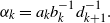 $\alpha_k=a_kb_k^{-1}d_{k+1}^{-1}.$
Proof. Clearly
 \begin{equation*} \xi_{n,n}=\frac{1}{y_{n,n}}=\frac{1}{a_n}=\frac{b_n^{-1}d_{n+1}^{-1}}{a_nb_n^{-1}d_{n+1}^{-1}}. \end{equation*}
For
 $1\le k< n$
, note that
 \begin{align} \xi_{k,n}&=\dfrac{y_{k+1,n}}{y_{k,n}} \notag \\ &=\dfrac{\mathbf{e}_1 B_{k+1}\cdots B_{n}\mathbf{e}_1^t}{\mathbf{e}_1 B_k\cdots B_{n}\mathbf{e}_1^t}\notag \\ &=\dfrac{\mathbf{e}_1 B_{k+1}\cdots B_{n}\mathbf{e}_1^t}{(a_k\mathbf{e}_1+b_k\mathbf{e}_2) B_{k+1}\cdots B_{n}\mathbf{e}_1^t}\notag\\ &=\dfrac{1}{a_k+b_k\frac{\mathbf{e}_2 B_{k+1}\cdots B_{n}\mathbf{e}_1^t}{\mathbf{e}_1 B_{k+1}\cdots B_{n}\mathbf{e}_1^t}}\notag \\ &=\dfrac{1}{a_k+b_kd_{k+1}\frac{\mathbf{e}_1 B_{k+2}\cdots B_{n}\mathbf{e}_1^t}{\mathbf{e}_1 B_{k+1}\cdots B_{n}\mathbf{e}_1^t}}\notag\\ &=\dfrac{b_k^{-1}d_{k+1}^{-1}}{a_kb_k^{-1}d_{k+1}^{-1}+\xi_{k+1,n}}. \end{align}
Thus the lemma can be proved by iterating (5.7).
With (5.5) and (5.6) in hand, Lemma 5.2 below, whose proof will be postponed to the end of this subsection, is crucial to the proof of Proposition 2.1.
Lemma 5.2. Let
 $\xi_k$
,
 $k\ge1$
,
 $\xi_{k,n}$
,
 $1\le k\le n$
, be as defined in (5.1)and (5.2)with
 $\beta_k=b_k^{-1}d_{k+1}^{-1}$
and
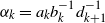 $\alpha_k=a_kb_k^{-1}d_{k+1}^{-1}$
,
 $k\ge1.$
Suppose condition (B1)and one of conditions (B2)
 $_a$
, (B2)
 $_b$
, and (B2)
 $_c$
hold. Then, as
 $n\rightarrow\infty$
, we have
 \begin{align} &\xi_{1,n}\cdots \xi_{n,n}\sim c\varrho(B_1)^{-1}\cdots\varrho(B_n)^{-1}, \end{align}
 \begin{align} &\xi_{1,n}\cdots \xi_{n,n}\sim c\xi_{1}\cdots \xi_{n}, \end{align}
 \begin{align} &\sum_{k=1}^{n+1}\xi_{1,n}\cdots\xi_{k-1,n}\sim c\sum_{k=1}^{n+1}\xi_{1}\cdots \xi_{k-1}. \end{align}
5.1.3. Estimations for the products of approximants of continued fractions by those of the tails
The proof of Lemma 5.2 depends heavily on the following lemma, which studies various properties of the continued fractions and their approximants.
Lemma 5.3. Let
 $\xi_{k,n}$
and
 $\xi_k$
be as defined in (5.1)and (5.2). Suppose that
 $\alpha_k,\beta_k>0$
for all
 $ k\ge1$
, and (5.3)is satisfied. Then we have
 \begin{align} &\xi_{k,n}\rightarrow\xi_k\in(0,\infty)\quad \text{as $ n\rightarrow\infty$,}\end{align}
 \begin{align} & \xi_{k,n}\begin{cases} <\xi_k& \text{if $ n-k+1 $ is even,} \\ \\[-7pt] >\xi_k&\text{if $ n-k+1$ is odd,} \end{cases}\quad 1\le k\le n,\end{align}
 \begin{align} &\xi_{k,n}\xi_{k+1,n} \begin{cases} >\xi_k\xi_{k+1}& \text{if $ n-k+1$ is even,} \\ \\[-7pt] <\xi_k\xi_{k+1}&\text{if $ n-k+1$ is odd,} \end{cases} \quad 1\le k\le n-1, \end{align}
 \begin{align} &\xi_k\cdots\xi_n\le \xi_{k,n}\cdots\xi_{n,n} \le \xi_k\cdots\xi_{n-1}\beta_n/\alpha_n,\quad n\ge k\ge1. \end{align}
Furthermore, if we assume in addition
 $\alpha_k\rightarrow \alpha>0$
,
 $\beta_k\rightarrow\beta>0.$
Then
 \begin{align} &\lim_{k\rightarrow\infty}\xi_k=\xi \,{:\!=}\, \dfrac{\sqrt{\alpha^2+4\beta}-\alpha}{2}>0,\end{align}
 \begin{align} & \xi\le1\Rightarrow\sum_{k=1}^{n}\xi_{1,n}\cdots\xi_{k,n}\sim \sum_{k=1}^{n}\xi_1\cdots\xi_{k}. \end{align}
Proof. Applying the Seidel–Stern theorem (see [Reference Lorentzen and Waadeland13, Theorem 3.14]) we get (5.11), and with (5.11) in hand, (5.12) is a direct consequence of [Reference Lorentzen and Waadeland13, Theorem 3.12]. Next, note that by (5.1) and (5.2) we have
 \begin{equation*} \xi_{k,n}\xi_{k+1,n}=\beta_k-\alpha_k\xi_{k,n} \quad\text{and}\quad \xi_k\xi_{k+1}=\beta_k-\alpha_k\xi_k\end{equation*}
respectively. Consequently
 \begin{equation*} \xi_{k,n}\xi_{k+1,n}- \xi_k\xi_{k+1}=\alpha_k(\xi_k-\xi_{k,n}),\end{equation*}
which together with (5.12) implies (5.13).
Next, we proceed to prove (5.14). We prove only the case when k is odd and n is even, since the other cases can be proved similarly. Noticing that
 $\xi_{n,n}={\beta_n}/{\alpha_n}$
, it then follows from (5.12) and (5.13) that
 \begin{align*} \xi_{k,n}\cdots\xi_{n,n}&=\xi_{k,n} \underline{\xi_{k+1,n}\xi_{k+2,n}}\cdots \underline{\xi_{n-2,n}\xi_{n-1,n}}\xi_{n,n}\le \xi_k\underline{\xi_{k+1}\xi_{k+2}}\cdots\underline{\xi_{n-2}\xi_{n-1}}\dfrac{\beta_n}{\alpha_n},\\[3pt] \xi_{k,n}\cdots\xi_{n,n}&=\underline{\xi_{k,n}\xi_{k+1,n}}\cdots \underline{\xi_{n-1,n}\xi_{n,n}}\ge \underline{\xi_k\xi_{k+1}}\cdots\underline{\xi_{n-1}\xi_{n}},\end{align*}
which imply (5.14).
The convergence of
 $\xi_k\rightarrow\xi>0$
in (5.15) follows from the convergence of the tails of the limit periodic continued fraction; see e.g. [Reference Lorentzen12, (4.2) on page 81].
Finally, we assume
 $\xi\le1$
to show (5.16). We claim that there exists
 $ N_0>0$
such that
 \begin{align} n-k+1\text{ is even } &\Rightarrow \dfrac{\xi_{k,n}-\xi_k}{\xi_{k+1}-\xi_{k+1,n}}< r\quad\text{for all $ n>k>N_0$,} \end{align}
 \begin{align} n-k+1\text{ is odd } &\Rightarrow \dfrac{\xi_{k,n}-\xi_k}{\xi_{k+2,n}-\xi_{k+2}}<r^2\quad\text{for all $n>k>N_0$,}\end{align}
where
 $0<r<1$
is a proper number.
In fact, since
 $\xi_k\rightarrow\xi\le1$
and
 $\alpha_k\rightarrow\alpha>0$
, then
 \begin{equation*} \frac{\xi_{k}}{\alpha_k+\xi_{k+1}}\rightarrow\frac{\xi}{\alpha+\xi}<1 \quad\text{as $k\rightarrow\infty.$} \end{equation*}
As a result, for a certain number
 $0<r<1$
, there exists
 $ N_0>0$
such that
 \begin{equation*} \frac{\xi_{k}}{\alpha_k+\xi_{k+1}}<r\quad \text{for all } k\ge N_0. \end{equation*}
On the other hand, it follows from (5.1) and (5.2) that
 \begin{equation*} \dfrac{\xi_{k,n}-\xi_k}{\xi_{k+1}-\xi_{k+1,n}}=\dfrac{\xi_{k,n}}{\alpha_k+\xi_{k+1}}=\dfrac{\xi_{k}}{\alpha_k+\xi_{k+1,n}}. \end{equation*}
If
 $n-k+1$
is even, then by (5.12) we have
 $\xi_{k+1,n}>\xi_{k+1}.$
Thus
 \begin{equation*} \dfrac{\xi_{k,n}-\xi_k}{\xi_{k+1}-\xi_{k+1,n}}=\dfrac{\xi_{k}}{\alpha_k+\xi_{k+1,n}}<\dfrac{\xi_{k}}{\alpha_k+\xi_{k+1}}<r\quad \text{for all $ n>k>N_0$.} \end{equation*}
If
 $n-k+1$
is odd, then by (5.13) we have
 $\xi_{k,n}\xi_{k+1,n}<\xi_k\xi_{k+1}.$
Therefore
 \begin{align*} \dfrac{\xi_{k,n}-\xi_k}{\xi_{k+2,n}-\xi_{k+2}} &=\dfrac{\xi_{k,n}}{\alpha_k+\xi_{k+1}}\dfrac{\xi_{k+1,n}}{\alpha_{k+1}+\xi_{k+2}} <\dfrac{\xi_{k}}{\alpha_k+\xi_{k+1}}\dfrac{\xi_{k+1}}{\alpha_{k+1}+\xi_{k+2}}<r^2\quad \text{for all $n\ge k>N_0$.} \end{align*}
We thus finish proving the claim.
Now we begin to prove (5.16). Again, we deal only with the case when n is an even number, since the other one follows similarly. Assume that n is an even number. Applying (5.12), (5.13) and checking carefully, we get
 \begin{align} \sum_{k=1}^{n}\xi_{1,n}\cdots\xi_{k,n}&=\xi_{1,n}+\xi_{1,n}\underline{\xi_{2,n}\xi_{3,n}}+ \cdots +\xi_{1,n} \underline{\xi_{2,n}\xi_{3,n}}\cdots \underline{\xi_{n-2,n}\xi_{n-1,n}}\notag\\&\quad\, +\xi_{1,n}\xi_{2,n}+\xi_{1,n}\underline{\xi_{2,n}\xi_{3,n}}\xi_{4,n}+ \cdots +\xi_{1,n} \underline{\xi_{2,n}\xi_{3,n}}\cdots \underline{\xi_{n-2,n}\xi_{n-1,n}}\xi_{n,n}\notag\\& \le \sum_{k=1}^{n}\xi_1\cdots\xi_{k}+\sum_{k=1}^{n/2}\prod_{i=1}^{2k-1}\xi_i(\xi_{2k,n}-\xi_{2k}).\end{align}
Since
 $n-2k+1$
is odd, we have
 $\xi_{2k,n}-\xi_{2k}>0$
and thus the second summation on the right-hand side of the above inequality is positive. Next we show that
 \begin{align} \lim_{n\rightarrow\infty}\dfrac{\sum_{k=1}^{n/2}\prod_{i=1}^{2k-1}\xi_i(\xi_{2k,n}-\xi_{2k})}{\sum_{k=1}^{n}\xi_1\cdots\xi_{k}}=0.\end{align}
To this end, fix
 $\varepsilon>0$
and let
 $N_1>0$
be an even number such that
 $r^{N_1}<\varepsilon.$
For convenience, we may assume
 $N_0$
in (5.17) and (5.18) is odd. Then
 \begin{align} \sum_{k=1}^{n/2}\prod_{k=1}^{2k-1}\xi_i(\xi_{2k,n}-\xi_{2k})&=\sum_{k=1}^{{(N_0-1)}/{2}} +\sum_{k={(N_0-1)}/{2}+1}^{{(n-N_1)}/{2}}+\sum_{k={(n-N_1)}/{2}+1}^{{n}/{2}}\prod_{i=1}^{2k-1}\xi_i(\xi_{2k,n}-\xi_{2k})\notag\\[3pt] & \,{=\!:}\, \mathrm{(I) +(II)+(III).}\end{align}
Since
 $\lim_{n\rightarrow\infty}\xi_{k,n}=\xi_k$
by (5.11), then the first term (I) on the right-hand side of (5.21) vanishes as
 $n\rightarrow\infty.$
Using the fact that
 $\lim_{k\rightarrow\infty}\xi_k \le 1$
and applying Lemma 4.2, for each
 $(n-N_1)\le i\le n/2$
, we have
 \begin{equation*}\frac{\xi_1\cdots\xi_{n-i}}{\sum_{k=1}^{n}\xi_1\cdots\xi_{k}}\rightarrow 0\quad\text{as $n\rightarrow\infty.$}\end{equation*}
Note also that
 $|\xi_{k,n}-\xi_{k}|<2\beta_k/\alpha_k<C$
for some universal constant
 $C>0.$
Therefore
 \begin{equation*}\lim_{n\rightarrow\infty}\mathrm{(III)}/\sum_{k=1}^{n}\xi_1\cdots\xi_{k}=0.\end{equation*}
Now we consider the term (II) on the right-hand side of (5.21). It follows from (5.18) that
 $\xi_{2k,n}-\xi_{2k}<r^{n-2k}(\xi_{n,n}-\xi_n)\le Cr^{n-2k}$
for some constant
 $C>0$
independent of n and k. Then we have
 \begin{align*}\dfrac{\mathrm{(II)}}{\sum_{k=1}^{n}\xi_1\cdots\xi_{k}}&= \sum_{k=(N_0-1)/2+1}^{(n-N_1)/2}\prod_{i=1}^{2k-1}\xi_i(\xi_{2k,n}-\xi_{2k})\Big/ \sum_{k=1}^{n}\xi_1\cdots\xi_{k}\\ &\le \sum_{k=(N_0-1)/2+1}^{(n-N_1)/2} Cr^{n-2k} <\sum_{k=N_1/2}^{\infty} Cr^{2k}\\ &=Cr^{N_1}/(1-r^2)<C\varepsilon/(1-r^2).\end{align*}
Since
 $\varepsilon$
is arbitrary, we get
 \begin{equation*}\lim_{n\rightarrow\infty}\frac{\mathrm{(II)}}{\sum_{k=1}^{n}\xi_1\cdots\xi_{k}}=0.\end{equation*}
Therefore we come to the conclusion that (5.20) is true. As a consequence, dividing by
 $\sum_{k=1}^{n}\xi_1\cdots\xi_{k}$
on both sides of (5.19) and taking the upper limit, we conclude that
 \begin{align} \varlimsup_{n\rightarrow\infty}\dfrac{\sum_{k=1}^{n}\xi_{1,n}\cdots\xi_{k,n}}{\sum_{k=1}^{n}\xi_1\cdots\xi_{k}}=1.\end{align}
For a lower limit, from (5.12), (5.13), and (5.17) we get
 \begin{align*} \sum_{k=1}^{n} \xi_{1,n}\cdots\xi_{k,n} & =\sum_{k=1}^{n/2}\underline{\xi_{1,n}\xi_{2,n}}\cdots \underline{\xi_{2k-3,n}\xi_{2k-2,n}}(\xi_{2k-1,n}-\xi_{2k-1})\\[3pt] &\quad\, +\sum_{k=1}^{n/2}\underline{\xi_{1,n}\xi_{2,n}}\cdots \underline{\xi_{2k-3,n}\xi_{2k-2,n}}\xi_{2k-1}+\sum_{k=1}^{n/2}\underline{\xi_{1,n}\xi_{2,n}}\cdots \underline{\xi_{2k-1,n}\xi_{2k,n}}\\[3pt] & \ge \sum_{k=1}^n \xi_1\xi_2\cdots\xi_k+\bigg(\sum_{k=1}^{N_0/2}+\sum_{k=N_0/2+1}^{n/2}\underline{\xi_{1}\xi_{2}}\cdots \underline{\xi_{2k-3}\xi_{2k-2}}(\xi_{2k,n}-\xi_{2k})\bigg). \end{align*}
Using (5.18), similarly to (5.20), we have
 \begin{equation*} \lim_{n\rightarrow\infty}\dfrac{\sum_{k=1}^{N_0/2}+\sum_{k=N_0/2+1}^{n/2}{\xi_{1}\xi_{2}}\cdots {\xi_{2k-3}\xi_{2k-2}}(\xi_{2k,n}-\xi_{2k})}{\sum_{k=1}^n \xi_1\xi_2\cdots\xi_k}=0. \end{equation*}
As a consequence,
 \begin{align} \varliminf_{n\rightarrow\infty}\dfrac{\sum_{k=1}^{n}\xi_{1,n}\cdots\xi_{k,n}}{\sum_{k=1}^{n}\xi_1\cdots\xi_{k}}=1.\end{align}
Taking (5.22) and (5.23) together, we get (5.16). The lemma is proved.
5.1.4. Fluctuations of the tails and critical tails of continued fractions
For
 $k\ge1$
, let
 \begin{align*} f_k&=\dfrac{ b_k d_k^{-1}}{ a_kd_k^{-1}} + \dfrac{ b_{k-1} d_{k-1}^{-1}}{ a_{k-1}d_{k-1}^{-1}} +\cdots+ \dfrac{ b_1 d_1^{-1}}{ a_1 d_1^{-1}},\\[3pt] \xi_k&=\dfrac{ b_k^{-1} d_{k+1}^{-1}}{ a_k b_k^{-1} d_{k+1}^{-1}} + \dfrac{ b_{k+1}^{-1} d_{k+2}^{-1}}{ a_{k+1}b_{k+1}^{-1}d_{k+2}^{-1}} +\cdots. \end{align*}
Further, set
 \begin{align*} \varepsilon^f_k&=f_k-b_{k+1}\varrho(B_{k+1})^{-1},\ \varepsilon^\xi_k=\xi_k-\varrho(B_{k})^{-1},\quad k\ge1,\\[3pt] \delta_k^f&=b_kd_k^{-1}-b_{k+1}\varrho(B_{k+1})^{-1}\left(a_kd_k^{-1}+b_{k}\varrho\left(B_{k}\right)^{-1}\right),\quad k\ge2,\\[3pt] \delta_k^\xi&=b_k^{-1}d_{k+1}^{-1}-\varrho(B_k)^{-1}\left(a_kb_k^{-1}d_{k+1}^{-1}+\varrho\left(B_{k+1}\right)^{-1}\right),\quad k\ge1.\end{align*}
Suppose that condition (B1) holds. Then, by the theory of convergence of limit periodic continued fractions (see [Reference Lorentzen12, (4.2) on page 81] and [Reference Lorentzen and Waadeland13, Theorem 4.13, page 188]), we have
 \begin{align} f_k\rightarrow b\varrho^{-1},\ \xi_k\rightarrow\varrho^{-1} \quad \text{and hence}\quad \varepsilon_k^f \rightarrow0,\ \varepsilon_k^\xi \rightarrow0 \quad\text{as $k\rightarrow\infty$.}\end{align}
Lemma 5.4 below studies the fluctuations of
 $\varepsilon_k^f$
and
 $\varepsilon_k^\xi$
,
 $k\ge1.$
Lemma 5.4. Suppose that condition (B1)and one of conditions (B2)
 $_{a}$
, (B2)
 $_{ b}$
, and (B2)
 $_{c}$
hold. Then there exists some number q with
 $|q|\le1$
such that
 \begin{align} &\lim_{k\rightarrow\infty}{\delta_{k+1}^f}/{\delta_k^f}=\lim_{k\rightarrow\infty}{\delta_{k+1}^\xi}/{\delta_k^\xi}=q,\end{align}
 \begin{align} &\lim_{k\rightarrow\infty}\dfrac{\varepsilon_{k+1}^\xi}{\varepsilon_{k}^\xi}=q,\quad \lim_{k\rightarrow\infty}\dfrac{\varepsilon_{k+1}^f}{\varepsilon_{k}^f}=q\quad\text{or}\quad -\dfrac{bd}{a\varrho+bd}.\end{align}
Proof. If (5.25) holds, then (5.26) is a direct consequence of [Reference Sun and Wang16, Lemma 4] and [Reference Lorentzen12, Theorem 6.1]. Therefore it is sufficient to prove (5.25).
Suppose condition (B1) holds. Then, by (5.24),
 $\lim_{k\rightarrow\infty} \delta_k^\xi=\lim_{k\rightarrow\infty} \delta_k^f=0.$
Thus, if the limits in (5.25) exist, we must have
 $|q|\le1.$
It remains to show that the limits in (5.25) exist and are equal. To this end, notice that by some direct computation we get
 \begin{equation*} \delta_k^f=\dfrac{b_kd_k^{-1}\Delta_k^f}{\frac{a_{k+1}}{b_{k+1}}+\sqrt{\bigl(\frac{a_{k+1}}{b_{k+1}}\bigr)^2+4\frac{d_{k+1}}{b_{k+1}}}}\quad\text{and}\quad \delta_k^\xi=\dfrac{b_k^{-1}d_{k+1}^{-1}\Delta_k^\xi}{\frac{a_{k}}{b_{k}}+\sqrt{\bigl(\frac{a_{k}}{b_{k}}\bigr)^2+4\frac{d_{k}}{b_{k}}}},\end{equation*}
where
 \begin{equation*}\Delta_k^f=\dfrac{a_{k+1}}{b_{k+1}}-\dfrac{a_{k}}{b_{k}}+\dfrac{\bigl(\frac{a_{k+1}}{b_{k+1}}-\frac{a_{k}}{b_{k}}\bigr)\bigl(\frac{a_{k+1}}{b_{k+1}}+\frac{a_{k}}{b_{k}}\bigr)+4\bigl(\frac{d_{k+1}}{b_{k+1}}-\frac{d_{k}}{b_{k}}\bigr)}{\sqrt{\bigl(\frac{a_{k+1}}{b_{k+1}}\bigr)^2+4\frac{d_{k+1}}{b_{k+1}}}+\sqrt{\bigl(\frac{a_{k}}{b_{k}}\bigr)^2+4\frac{d_{k}}{b_{k}}}}\end{equation*}
and
 \begin{equation*}\Delta_k^\xi=\dfrac{a_{k+1}}{b_{k+1}}-\dfrac{a_{k}}{b_{k}}-\dfrac{\bigl(\frac{a_{k+1}}{b_{k+1}}-\frac{a_{k}}{b_{k}}\bigr)\bigl(\frac{a_{k+1}}{b_{k+1}}+\frac{a_{k}}{b_{k}}\bigr)+4\bigl(\frac{d_{k+1}}{b_{k+1}}-\frac{d_{k}}{b_{k}}\bigr)}{\sqrt{\bigl(\frac{a_{k+1}}{b_{k+1}}\bigr)^2+4\frac{d_{k+1}}{b_{k+1}}}+\sqrt{\bigl(\frac{a_{k}}{b_{k}}\bigr)^2+4\frac{d_{k}}{b_{k}}}}.\end{equation*}
Therefore, by condition (B1), we have
 \begin{equation*}\lim_{k\rightarrow\infty}{\delta_{k+1}^f}/{\delta_k^f}=\lim_{k\rightarrow\infty}{\Delta_{k+1}^f}/{\Delta_k^f},\quad \lim_{k\rightarrow\infty}{\delta_{k+1}^\xi}/{\delta_k^\xi}=\lim_{k\rightarrow\infty}{\Delta_{k+1}^\xi}/{\Delta_k^\xi}. \end{equation*}
Suppose now that condition (B2)
 $_{a}$
holds. Then the limits
 \begin{equation*}\lim_{k\rightarrow\infty}{\delta_{k+1}^f}/{\delta_k^f}=\lim_{k\rightarrow\infty}{\delta_{k+1}^\xi}/{\delta_k^\xi}=\lim_{k\rightarrow\infty}\dfrac{d_{k+2}/b_{k+2}-d_{k+1}/b_{k+1}}{d_{k+1}/b_{k+1}-d_{k}/b_{k}}\end{equation*}
exist. Next, suppose that condition (B2)
 $_{b}$
holds. Then the limits
 \begin{equation*}\lim_{k\rightarrow\infty}{\delta_{k+1}^f}/{\delta_k^f}=\lim_{k\rightarrow\infty}{\delta_{k+1}^\xi}/{\delta_k^\xi}=\lim_{k\rightarrow\infty}\dfrac{a_{k+2}/b_{k+2}-a_{k+1}/b_{k+1}}{a_{k+1}/b_{k+1}-a_{k}/b_{k}}\end{equation*}
exist. Finally, suppose condition (B2)
 $_{ c}$
holds. If
 \begin{equation*}\tau \,{:\!=}\, \lim_{k\rightarrow\infty}\dfrac{d_{k+1}/b_{k+1}-d_{k}/b_k}{a_{k+1}/b_{k+1}-a_{k}/b_k}\ne \dfrac{-a\pm \sqrt{a^2+4bd}}{2b} \end{equation*}
is finite, then
 \begin{align*} &\lim_{k\rightarrow\infty}\dfrac{\Delta_k^f}{\frac{a_{k+1}}{b_{k+1}}-\frac{a_{k}}{b_{k}}} =1-\dfrac{a/b+2\tau}{\sqrt{(a/b)^2+4d/b}}\ne 0,\\ &\lim_{k\rightarrow\infty}\dfrac{\Delta_k^\xi}{\frac{a_{k+1}}{b_{k+1}}-\frac{a_{k}}{b_{k}}} =1+\dfrac{a/b+2\tau}{\sqrt{(a/b)^2+4d/b}}\ne 0\end{align*}
and consequently the limits
 \begin{equation*} \lim_{k\rightarrow\infty}{\delta_{k+1}^f}/{\delta_k^f}=\lim_{k\rightarrow\infty}{\delta_{k+1}^\xi}/{\delta_k^\xi}=\lim_{k\rightarrow\infty}\dfrac{a_{k+2}/b_{k+2}-a_{k+1}/b_{k+1}}{a_{k+1}/b_{k+1}-a_{k}/b_{k}} \end{equation*}
exist. Otherwise, if
 $\tau$
is infinite, then
 \begin{equation*}\lim_{k\rightarrow\infty}\frac{a_{k+1}/b_{k+1}-a_{k}/b_k}{d_{k+1}/b_{k+1}-d_{k}/b_k}=0\end{equation*}
and hence
 \begin{equation*}\lim_{k\rightarrow\infty}{\delta_{k+1}^f}/{\delta_k^f}=\lim_{k\rightarrow\infty}{\delta_{k+1}^\xi}/{\delta_k^\xi}=\lim_{k\rightarrow\infty}\dfrac{d_{k+2}/b_{k+2}-d_{k+1}/b_{k+1}}{d_{k+1}/b_{k+1}-d_{k}/b_{k}}\end{equation*}
exist. The lemma is proved.
We are now ready to prove Lemma 5.2.
5.1.5. Proof of Lemma 5.2
Proof. Suppose now that condition (B1) and one of conditions (B2)
 $_a$
, (B2)
 $_b$
, and (B2)
 $_c$
hold. Then Lemma 5.4 allows us to apply [Reference Sun and Wang16, Theorem 1] to
 $B_k^t$
,
 $k\ge1$
, to yield that for
 $i,j\in\{1,2\}$
and
 $m\ge 1$
, there exists a number
 $0<c(m)<\infty$
such that
 \begin{align} \mathbf{e}_iB_m\cdots B_n\mathbf{e}_j^t =\mathbf{e}_jB_n^t\cdots B_m^t\mathbf{e}_i^t\sim c(m)\varrho(B_m)\cdots \varrho(B_n) \quad \text{as $n\rightarrow\infty$.}\end{align}
Here we remark that when considering
 $B_k^t$
,
 $k\ge1$
, conditions (B2)
 $_a$
, (B2)
 $_b$
, and (B2)
 $_c$
in this paper are slightly different from their counterparts in [Reference Sun and Wang16]. But the key role which (B2)
 $_a$
, (B2)
 $_b$
, and (B2)
 $_c$
in [Reference Sun and Wang16] play is to show that
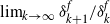 $\lim_{k\rightarrow\infty}{\delta_{k+1}^f}/{\delta_k^f}$
exists. Lemma 5.4 showed that
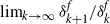 $\lim_{k\rightarrow\infty}{\delta_{k+1}^f}/{\delta_k^f}$
does exist under one of conditions (B2)
 $_a$
, (B2)
 $_b$
, and (B2)
 $_c$
of this paper. So we can apply [Reference Sun and Wang16, Theorem 1] to
 $B_k^t$
,
 $k\ge1$
, to get (5.27).
By Lemma 5.1, for
 $1\le k\le n$
,
 $\xi_{k,n}$
in (5.1) coincides with the one in (5.4), if
 $\beta_k=b_k^{-1}d_{k+1}^{-1}$
and
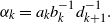 $\alpha_k=a_kb_k^{-1}d_{k+1}^{-1}.$
Therefore, from (5.5) and (5.27) we get
 \begin{align} \xi_{1,n}\cdots \xi_{n,n}=\dfrac{1}{\mathbf{e}_1B_1\cdots B_n\mathbf{e}_1^t}\sim c\varrho(B_1)^{-1}\cdots \varrho(B_n)^{-1} \quad \text{as $n\rightarrow\infty$,}\end{align}
which finishes the proof of (5.8).
In order to prove (5.9), noticing that
 $\lim_{k\rightarrow\infty}\beta_k=b^{-1}d^{-1}$
and
 $\lim_{k\rightarrow\infty}\alpha_k=ab^{-1}d^{-1}$
, thus (5.3) is fulfilled. Therefore, by Lemma 5.3, we have for
 $k\ge1$
,
 \begin{equation*} \xi_{k,n}\rightarrow\xi_k\in(0,\infty)\quad \text{as $ n\rightarrow\infty$,} \end{equation*}
and for
 $n\ge1$
,
 \begin{align} &1\le \dfrac{\xi_{1,n}\cdots\xi_{n,n}}{\xi_1\cdots\xi_n} \le \dfrac{\beta_n}{\xi_n\alpha_n}. \end{align}
To prove (5.9), in view of (5.8), it suffices to show that
 \begin{align} \xi_1\cdots\xi_n\sim c\varrho(B_1)^{-1}\cdots \varrho(B_n)^{-1}\quad \text{as $n\rightarrow\infty$.}\end{align}
To this end, write
 \begin{equation*}x_n=\frac{\xi_1\cdots\xi_n}{\varrho(B_1)^{-1}\cdots\varrho(B_n)^{-1}},\quad n\ge1,\end{equation*}
noting that by (5.28) and (5.29), there exist
 $0< c_3\le c_4<\infty$
such that
 \begin{equation} c_3\le x_k\le c_4\quad\text{for all $ k\ge1$.}\end{equation}
Notice that, by Lemma 5.4,
 \begin{align} \lim_{k\rightarrow\infty}\dfrac{\xi_{k+1}-\varrho(B_{k+1})^{-1}}{\xi_{k}-\varrho(B_{k})^{-1}}=q\end{align}
for some number q with
 $|q|\le1.$
First we suppose
 $|q|<1.$
Then it follows from (5.32) that
 $\sum_{k=1}^{\infty}\left|\xi_k-\varrho\left(B_k\right)^{-1}\right|<\infty.$
Since
 $\lim_{n\rightarrow\infty}\varrho(B_n)=\varrho$
, taking (5.31) into account, we have
 \begin{align} \sum_{n=1}^\infty|x_{n+1}-x_{n}|&=\sum_{n=1}^{\infty}\varrho(B_{n+1})x_n\left|\xi_{n+1}-\varrho\left(B_{n+1}\right)^{-1}\right|\notag\\ &\le c\sum_{n=1}^{\infty}\left|\xi_{n+1}-\varrho\left(B_{n+1}\right)^{-1}\right|<\infty.\end{align}
Therefore, by (5.31) and (5.33), we have
 $\lim_{k\rightarrow\infty}x_k=c$
for some
 $c>0.$
Second, we suppose
 $q=1.$
Then there exists a number
 $k_3>0$
such that
 \begin{align} \text{ either }\xi_k-\varrho(B_k)^{-1} \ge 0\quad\text{for all $ k\ge k_3$} \quad \text{or}\quad \xi_k-\varrho(B_k)^{-1} \le 0 \quad\text{for all $ k\ge k_3$.}\end{align}
But for
 $k\ge1$
we have
 \begin{equation*}\frac{x_{k+1}}{x_k}=\frac{\xi_{k+1}}{\varrho(B_{k+1})^{-1}},\end{equation*}
so that by (5.34), we must have either
 $x_{k+1}\le x_k$
for all
 $ k\ge k_3$
or
 $x_{k+1}\ge x_k$
for all
 $ k\ge k_3.$
That is,
 $x_k$
,
 $k\ge k_3$
, is monotone in k. This fact together with (5.31) implies
 $\lim_{k\rightarrow\infty}x_k=c$
for some number
 $c>0.$
Finally we suppose
 $q=-1.$
Then there exists a number
 $k_4>0$
such that
 \begin{equation*} \dfrac{\xi_{k+1}-\varrho(B_{k+1})^{-1}}{\xi_{k}-\varrho(B_{k})^{-1}}<0\quad \text{for all $ k\ge k_4$.} \end{equation*}
Thus
 $\xi_{k}-\varrho(B_{k})^{-1}$
,
 $k\ge k_4$
, converges to 0 in an alternate manner as
 $k\rightarrow\infty.$
Therefore
 \begin{equation*} \lim_{k\rightarrow\infty}x_k=\lim_{k\rightarrow\infty}\biggl(x_1+\sum_{i=2}^{k}(x_k-x_{k-1})\biggr)=c\quad\text{for some }c>0. \end{equation*}
We have shown that in any case
 $\lim_{k\rightarrow\infty}x_k=c$
for some
 $c>0.$
Consequently (5.30) is proved and so is (5.9).
Finally we give the proof of (5.10). If
 $\varrho\ge1$
, then by (5.24),
 $\xi=\varrho^{-1}\le1.$
Thus, applying Lemma 5.3, from (5.16), we get (5.10).
Therefore we now assume
 $\varrho<1.$
Since
 $\lim_{k\rightarrow\infty}\xi_k=\varrho^{-1}$
by (5.24), applying Lemma 4.2 to
 $\xi_k$
,
 $k\ge1$
, we get
 \begin{align} \lim_{n\rightarrow\infty}\dfrac{\xi_1\cdots\xi_{n+1}}{\sum_{k=1}^{n+1}\xi_1\cdots\xi_{k-1}} =\begin{cases} 0 & \text{if $\varrho\ge 1$,} \\ \\[-7pt] \varrho^{-1}-1 & \text{if $\varrho< 1$.} \end{cases} \end{align}
It follows from (5.6), (5.9), and (5.35) that
 \begin{equation*} \sum_{k=1}^{n+1} \mathbf{e}_1B_k\cdots B_n\mathbf{e}_1^t=\dfrac{\sum_{k=1}^{n+1} \xi_{1,n}\cdots \xi_{k-1,n}}{\xi_{1,n}\cdots \xi_{n,n}}\sim c\dfrac{\sum_{k=1}^{n+1}\xi_{1,n}\cdots\xi_{k-1,n}}{\sum_{k=1}^{n+1}\xi_1\cdots\xi_{k-1}}\quad\text{as $n\rightarrow\infty.$} \end{equation*}
Thus, to prove (5.10), it is sufficient to show that
 \begin{align} \lim_{n\rightarrow\infty}\sum_{k=1}^{n+1} \mathbf{e}_1B_k\cdots B_n\mathbf{e}_1^t=c \end{align}
for some number
 $c>0.$
Notice that by (5.5) and (5.14), we have for
 $n\ge m\ge1$
 \begin{align} c_5\xi_m^{-1}\cdots \xi_n^{-1} <\mathbf{e}_1B_m\cdots B_n\mathbf{e}_1^t <c_6\xi_m^{-1}\cdots \xi_n^{-1} ,\end{align}
where
 $0<c_5<c_6<\infty$
are some numbers independent of n and m. Since
 $\xi_k^{-1}\rightarrow\varrho<1$
as
 $k\rightarrow\infty$
, fixing
 $0\le \varepsilon_0 <(1-\varrho)\wedge\varrho$
, there exists a number
 $n_0>0$
such that
 \begin{align} \varrho-\varepsilon_0<\xi_k^{-1}<\varrho+\varepsilon_0\quad\text{for all $k\ge n_0$.}\end{align}
Now fix
 $\varepsilon>0$
and let
 $n_1$
be a number large enough so that
 $(\varrho+\varepsilon_0)^{n_1}<\varepsilon.$
For
 $n\ge1$
, use the notation
 $y_{k,n}=\mathbf{e}_1B_k\cdots B_n\mathbf{e}_1^t$
and write
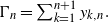 $\Gamma_n=\sum_{k=1}^{n+1} y_{k,n}.$
We have
 \begin{align} |\Gamma_{n+1}-\Gamma_n| & =\biggl|y_{1,n+1}+\sum_{k=1}^{n}(y_{k+1,n+1}-y_{k,n})\biggr|\notag\\[3pt] &\le y_{1,n}+\biggl|\sum_{k=1}^{n_0-1}(y_{k+1,n+1}-y_{k,n})\biggr|+\biggl|\sum_{k=n_0}^{n-n_1}(y_{k+1,n+1}-y_{k,n})\biggr| \notag\\[3pt] &\quad\, +\biggl|\sum_{k=n-n_1+1}^{n}(y_{k+1,n+1}-y_{k,n})\biggr|\notag\\[3pt] & \,{=\!:}\, \mathrm{(I)+(II)+(III)+(IV)}.\end{align}
Since
 $\varrho<1$
, for each
 $k\ge1$
, by (5.27) we have
 $\lim_{n\rightarrow\infty}y_{k,n}=0.$
Also, for any
 $m\ge 1$
, the fact that
 $\lim_{n\rightarrow\infty}B_n=B$
implies that
 $y_{n-m,n}-y_{n-m+1,n+1}\rightarrow 0$
as
 $n\rightarrow\infty.$
Thus (I), (II), and (IV) on the right-hand side of (5.39) vanish as
 $n\rightarrow\infty.$
We claim that (III) on the right-hand side of (5.39) also vanishes. Indeed, from (5.37) we obtain
 $y_{k,n}\le c_6\xi_k^{-1}\cdots \xi_n^{-1}$
for all
 $n\ge k\ge1.$
Therefore, taking (5.38) into account,
 \begin{align*} \mathrm{(III)}&\le \sum_{k=n_0}^{n-n_1}(|y_{k+1,n+1}|+|y_{k,n}|) \\ &\le 2 c_6 \sum_{k=n_0}^{n-n_1}(\varrho+\varepsilon_0)^{n-k+1}\\ &\le 2c_6\sum_{k=n_1+1}^{\infty}(\varrho+\varepsilon_0)^k\\ &=2c_6\dfrac{(\varrho+\varepsilon_0)^{n_1+1}}{1-(\varrho+\varepsilon_0)}\\ &\le \dfrac{2c_6\varepsilon}{1-(\varrho+\varepsilon_0)}.\end{align*}
Thus we can conclude that
 \begin{align} \lim_{n\rightarrow\infty}(\Gamma_{n+1}-\Gamma_n)=0.\end{align}
But by (5.37), we have
 \begin{align} c_7<\Gamma_{n}<c_8\quad \text{for all $ n\ge 1$,}\end{align}
where
 $0<c_7<c_8<\infty$
are some constants independent of n. Therefore, taking (5.40) and (5.41) together, we get
 \begin{align} \lim_{n\rightarrow\infty}\dfrac{\Gamma_{n+1}}{\Gamma_n}=1.\end{align}
For
 $n\ge1$
, set
 \begin{equation*} f_n\equiv \dfrac{\mathbf{e}_1\prod_{k=1}^{n}B_{k}\mathbf{e}_2^t}{\mathbf{e}_1\prod_{k=1}^{n} B_{k}\mathbf{e}_1^t} \quad\text{and}\quad H_n\equiv\sum_{k=1}^{n}\mathbf{e}_1\prod_{i=k}^{n} B_{i}(f_n\mathbf{e}_1^t-\mathbf{e}_2^t). \end{equation*}
Since
 $\varrho<1$
, we can apply Lemma 4.1 (with
 $\theta=0$
) to get
 \begin{align} \lim_{n\rightarrow\infty}f_n=-\dfrac{\varrho_1(B)}{d} \quad\text{and}\quad \lim_{n\rightarrow\infty}H_n=-\dfrac{1}{d }\dfrac{\varrho_1(B)^2}{1-\varrho_1(B)}. \end{align}
Noticing that
 \begin{align} H_n&=(\Gamma_n-1)f_n-\sum_{k=1}^n\mathbf{e}_1 B_k\cdots B_{n}\mathbf{e}_2^t \notag\\ &=(\Gamma_n-1)f_n-b_n\biggl(\sum_{k=1}^{n}\mathbf{e}_1 B_k\cdots B_{n-1}\mathbf{e}_1^t\biggr)\notag \\ &=\Gamma_nf_n-b_n\Gamma_{n-1}-f_n, \notag \end{align}
it thus follows from (5.42) and (5.43) that
 \begin{equation*} \lim_{n\rightarrow\infty}\Gamma_n=\lim_{n\rightarrow\infty} \dfrac{H_n+f_n}{f_n-b_n\Gamma_{n-1}/\Gamma_n}=\dfrac{\varrho_1(B)}{(\varrho_1(B)+bd)(1-\varrho_1(B))}>0,\end{equation*}
where to show the positivity of the limit we use the fact
 $\varrho<1.$
Consequently (5.36) is proved. Thus (5.10) is true and we complete the proof of Lemma 5.2.
5.2. Proof of Proposition 2.1
Proof. We are now ready to complete the proof of Proposition 2.1. Suppose condition (B1) and one of conditions (B2)
 $_a$
, (B2)
 $_b$
, and (B2)
 $_c$
hold. Then (2.15) is a direct consequence of (5.27) above. Furthermore, it follows from (5.6) that
 \begin{align*} Y_n&=\dfrac{\varrho(B_1)^{-1}\cdots\varrho(B_n)^{-1}}{\xi_{1,n}\cdots\xi_{n,n}}\dfrac{\sum_{k=1}^{n+1}\xi_{1,n}\cdots \xi_{k-1,n}}{\sum_{k=1}^{n+1}\xi_{1}\cdots \xi_{k-1}} \dfrac{\sum_{k=1}^{n+1}\xi_{1}\cdots \xi_{k-1}}{\sum_{k=1}^{n+1}\varrho(B_1)^{-1}\cdots\varrho(B_{k-1})^{-1}}\\ & \,{=\!:}\, T_1(n)\times T_2(n)\times T_3(n). \end{align*}
Notice that by (5.8), (5.9), and (5.10), for
 $i=1,2,3$
, we have
 \begin{align}\lim_{n\rightarrow\infty}T_i(n)=T_i\end{align}
for some number
 $T_i\in (0,\infty).$
Therefore
 $\lim_{n\rightarrow\infty}Y_n=T_1T_2T_3.$
Consequently, with
 \begin{align} \psi \,{:\!=}\, T_1T_2T_3\in(0,\infty),\end{align}
Appendix A. Proof of Lemma 2.1
Proof. Since
 \begin{equation*} \lim_{n\rightarrow\infty}\frac{r_n-r_{n+1}}{r_n^2}=c \end{equation*}
for some number
 $0<c<\infty$
, we must have
 $\lim_{n\rightarrow\infty}{r_{n+1}}/{r_n}=1$
and there exists a number
 $N_0$
such that for all
 $ n\ge N_0$
,
 $r_{n+1}<r_n.$
Consequently condition (B1) holds. Next we show that one of conditions (B2)
 $_{ a}$
, (B2)
 $_{ b}$
, and (B2)
 $_{ c}$
holds.
Case 1: Assume that
 $a=b=\theta\ne d.$
Recall that by assumption
 $b>0.$
Thus, for all
 $k\ge1$
,
 \begin{equation*}\frac{\tilde a_k}{\tilde b_k}=\frac{a_k}{b_k}+\frac{\theta_{k+1}}{b_{k+1}}=\frac{a+r_k}{b+r_k}+\frac{\theta+r_{k+1}}{b+r_{k+1}}\equiv 2.\end{equation*}
That is, for all
 $ k\ge1$
,
 \begin{equation*}\frac{\tilde a_k}{\tilde b_k}=\frac{\tilde a_{k+1}}{\tilde b_{k+1}}.\end{equation*}
Moreover, notice that
 \begin{align} \dfrac{\,\tilde{\!d}_k}{\tilde b_k}&=\dfrac{d_kb_k-a_k\theta_k}{b_k^2}=\dfrac{(d+r_k)(b+r_k)-(a+r_k)(\theta+r_k)}{(b+r_k)^2}\notag\\ &=\dfrac{bd-a\theta+(b+d-a-\theta)r_k}{(b+r_k)^2},\quad k\ge1.\end{align}
Writing
 \begin{equation*}g(x) \,{:\!=}\, \dfrac{bd-a\theta+(b+d-a-\theta)x}{(b+x)^2},\quad x\ge 0,\end{equation*}
we have
 \begin{align} g'(x)=\dfrac{b(b+d-a-\theta)+2(a\theta-bd)-(b+d-a-\theta)x}{(b+x)^3}.\end{align}
Since
 $a=b=\theta\ne d$
, we get
 $g'(0)={b(b-d)}/{b^3}\ne 0.$
Thus, for some
 $k_0>0$
,
 ${\,\tilde{\!d}_k}/{\tilde b_k}$
,
 $k\ge k_0$
, is monotone in k. That is,
 $\,\tilde{\!d}_{k}/\tilde b_{k}\ne\,\tilde{\!d}_{k+1}/\tilde b_{k+1}$
,
 $k\ge k_0.$
On the other hand, for any numbers
 $\alpha,\beta\in \mathbb R$
with
 $\beta=0$
, we have
 \begin{align} \dfrac{\alpha+x}{\beta+x}=\dfrac{\alpha}{\beta}+\dfrac{\beta-\alpha}{\beta^2}x-\dfrac{\beta-\alpha}{\beta^3}x^2+{\mathrm{o}}(x^2) \quad\text{as $x\rightarrow0.$}\end{align}
Thus we get
 \begin{equation*} \,\tilde{\!d}_k/\tilde b_k=\dfrac{d+r_k}{b+r_k}-1=\dfrac{d}{b}-1 +\dfrac{b-d}{b^2}r_k-\dfrac{b-d}{b^3}r_k^2+{\textrm{o}}(r_k^2).\end{equation*}
As a result, using the fact
 $r_{n}\sim r_{n+1}$
and
 $r_n-r_{n+1}\sim cr_n^2$
as
 $n\rightarrow\infty$
, we get
 \begin{equation*}\lim_{k\rightarrow\infty}\dfrac{\,\tilde{\!d}_{k+2}/\tilde b_{k+2}-\,\tilde{\!d}_{k+1}/\tilde b_{k+1}}{\,\tilde{\!d}_{k+1}/\tilde b_{k+1}-\,\tilde{\!d}_{k}/\tilde b_{k}}=1.\end{equation*}
We thus come to the conclusion that condition (B2)
 $_{ a}$
is satisfied.
Case 2: Suppose that a, b and
 $\theta$
are not all equal. In this case, since
 $(b-a)(b-\theta)\ge0$
, then for some number
 $k_0>0$
,
 \begin{equation*}\tilde a_k/\tilde b_k=\dfrac{a+r_k}{b+r_k}+\dfrac{\theta+r_{k+1}}{b+r_{k+1}},\quad k\ge k_0\end{equation*}
is monotone in k. That is,
 $\tilde a_k/\tilde b_k\ne \tilde a_{k+1}/\tilde b_{k+1}$
,
 $k\ge k_0.$
In the first place, if
 $b+d-a-\theta=0$
and
 $a\theta-bd=0$
, then it follows from (A.1) that
 $\,\tilde{\!d}_k/\tilde b_k=\,\tilde{\!d}_{k+1}/\tilde b_{k+1}=0$
for all
 $ k\ge1.$
Using (A.3), we get
 \begin{align} \dfrac{\tilde a_{k+2}}{\tilde b_{k+2}}- \dfrac{\tilde a_{k+1}}{\tilde b_{k+1}}=\dfrac{b-a}{b^2}(r_{k+2}-r_{k+1})+\dfrac{b-\theta}{b^2}(r_{k+3}-r_{k+2})+{\textrm{o}}(r_{k}^2).\end{align}
Since
 $a,b,\theta$
are not all equal and
 $(b-a)(b-\theta)\ge0$
, we have
 $(b-a)/b^2+(b-\theta)/b^2\ne0.$
Consequently we get
 \begin{equation*}\lim_{k\rightarrow\infty}\frac{\tilde a_{k+2}/\tilde b_{k+2}-\tilde a_{k+1}/\tilde b_{k+1}}{\tilde a_{k+1}/\tilde b_{k+1}-\tilde a_{k}/\tilde b_{k+1}}=1.\end{equation*}
Therefore condition (B2)
 $_{ b}$
holds.
In the second place, suppose that
 $b+d-a-\theta$
and
 $a\theta-bd$
are not 0 simultaneously. Then, from (A.1) and (A.2), we have that
 $\,\tilde{\!d}_k/\tilde b_k$
,
 $k\ge k_0$
is monotone in k for some number
 $k_0>0$
, i.e.
 $\,\tilde{\!d}_k/\tilde b_k\ne \,\tilde{\!d}_{k+1}/\tilde b_{k+1}$
,
 $k\ge k_0.$
But it follows from (A.1) and (A.3) that
 \begin{equation*} \dfrac{\,\tilde{\!d}_{k+1}}{\tilde b_{k+1}}-\dfrac{\,\tilde{\!d}_{k}}{\tilde b_k}=\biggl(\dfrac{b-d}{b^2}-\dfrac{a(b-\theta)+\theta(b-a)}{b^3}\biggr)(r_{k+1}-r_k)+{\textrm{o}}(r_k^2).\end{equation*}
Since
 $(b-\theta)(b-a)\ge0$
and
 $a,b,\theta$
are not all equal, taking (A.4) into account, we get
 \begin{align*}&\lim_{k\rightarrow\infty}\dfrac{\tilde a_{k+2}/\tilde b_{k+2}-\tilde a_{k+1}/\tilde b_{k+1}}{\tilde a_{k+1}/\tilde b_{k+1}-\tilde a_{k}/\tilde b_{k+1}}=1,\\[3pt] &\lim_{k\rightarrow\infty}\dfrac{\,\tilde{\!d}_{k+1}/\tilde b_{k+1}-\,\tilde{\!d}_{k}/\tilde b_k}{\tilde a_{k+1}/\tilde b_{k+1}-\tilde a_{k}/\tilde b_k}=\dfrac{b(b+d-a-\theta)+2(a\theta-bd)}{b(b-a)+b(b-\theta)} \,{=\!:}\, \tau ,\end{align*}
which is finite, and by assumption
 \begin{equation*}\tau \ne \frac{-(a+\theta) \pm \sqrt{(a+\theta)^2+4(bd-a\theta)}}{2b}.\end{equation*}
Thus we conclude that condition (B2)
 $_{c}$
holds. Lemma 2.1 is proved.
Remark A.1. Note that Lemma 2.1 excludes the case
 $a=b=\theta=d$
, which is trivial. Indeed, in this case,
 \begin{equation*} M_k=(a+r_k) \begin{pmatrix} 1&\,\, 1 \\ \\[-7pt] 1 &\,\, 1 \\ \end{pmatrix} \end{equation*}
and thus
 \begin{equation*} M_1\cdots M_n=(a+r_1)\cdots (a+r_n) \begin{pmatrix} 2^{n-1}&\,\, 2^{n-1} \\ \\[-7pt] 2^{n-1} &\,\, 2^{n-1}\\ \end{pmatrix}\!,\quad n\ge1.\end{equation*}
Acknowledgements
The authors would like to thank Professor W. M. Hong for introducing to us the basics of BPVEs, and Professor V. Vatutin for some discussions on the distribution of the extinction time when writing the paper. Finally, the authors are in debt to two referees who read the paper carefully and gave very good suggestions which helped to improve the paper to a large extent.
Funding information
This project is partially supported by the National Natural Science Foundation of China (grant 12071003; 11501008).
Competing interests
There were no competing interests to declare which arose during the preparation or publication process of this article.


