2 Derivation of the asymptotic reduced model

2.1 Linearized equations for the interaction

The Euler equations governing the dynamics of a compressible homentropic fluid are

(2.1a ) $$\begin{eqnarray}\displaystyle & \displaystyle \frac{\unicode[STIX]{x2202}\boldsymbol{v}}{\unicode[STIX]{x2202}t}+\boldsymbol{v}\boldsymbol{\cdot }\unicode[STIX]{x1D735}\boldsymbol{v}+\frac{1}{\unicode[STIX]{x1D70C}}\unicode[STIX]{x1D735}p=0, & \displaystyle\end{eqnarray}$$

(2.1b ) $$\begin{eqnarray}\displaystyle & \displaystyle \frac{\unicode[STIX]{x2202}\unicode[STIX]{x1D70C}}{\unicode[STIX]{x2202}t}+\unicode[STIX]{x1D735}\boldsymbol{\cdot }(\unicode[STIX]{x1D70C}\boldsymbol{v})=0, & \displaystyle\end{eqnarray}$$

(2.1c ) $$\begin{eqnarray}\displaystyle & \displaystyle \frac{p}{\unicode[STIX]{x1D70C}^{\unicode[STIX]{x1D6FE}}}=\text{const.}, & \displaystyle\end{eqnarray}$$

where $(\boldsymbol{v},p,\unicode[STIX]{x1D70C})$ denote velocity, pressure and density, respectively, and $\unicode[STIX]{x1D6FE}$ is the ratio of specific heats. We consider a weak acoustic wave field, $(\boldsymbol{v}^{\prime },p^{\prime },\unicode[STIX]{x1D70C}^{\prime })$ propagating through a steady incompressible vortical flow $(\overline{\boldsymbol{v}}(\boldsymbol{x}),\overline{p}(\boldsymbol{x}),\overline{\unicode[STIX]{x1D70C}})$ that satisfies the incompressible Euler equations:

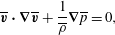(2.2a ) $$\begin{eqnarray}\displaystyle & \displaystyle \overline{\boldsymbol{v}}\boldsymbol{\cdot }\unicode[STIX]{x1D735}\overline{\boldsymbol{v}}+\frac{1}{\overline{\unicode[STIX]{x1D70C}}}\unicode[STIX]{x1D735}\overline{p}=0, & \displaystyle\end{eqnarray}$$

(2.2b ) $$\begin{eqnarray}\displaystyle & \displaystyle \unicode[STIX]{x1D735}\boldsymbol{\cdot }\overline{\boldsymbol{v}}=0, & \displaystyle\end{eqnarray}$$

where $\overline{\unicode[STIX]{x1D70C}}$ is constant. (We note that demanding the vortical flow to be ‘steady’ is slightly over-restrictive. Strictly speaking we can let the vortical flow evolve on a slow time scale as long as $L/U$ is asymptotically greater than $\unicode[STIX]{x1D714}^{-1}$ so that the wave field satisfies the ‘high-frequency’ requirement.) Using the vortex–wave splitting $\boldsymbol{v}=\overline{\boldsymbol{v}}+a\boldsymbol{v}^{\prime },~p=\overline{p}+ap^{\prime },~\unicode[STIX]{x1D70C}=\overline{\unicode[STIX]{x1D70C}}+a\unicode[STIX]{x1D70C}^{\prime }$ in (2.1), where $a\ll 1$ is the wave amplitude, and ignoring the nonlinear wave interaction terms of $O(a^{2})$ , we get

(2.3a ) $$\begin{eqnarray}\displaystyle & \displaystyle \frac{\unicode[STIX]{x2202}\boldsymbol{v}^{\prime }}{\unicode[STIX]{x2202}t}+\boldsymbol{v}^{\prime }\boldsymbol{\cdot }\unicode[STIX]{x1D735}\overline{\boldsymbol{v}}+\overline{\boldsymbol{v}}\boldsymbol{\cdot }\unicode[STIX]{x1D735}\boldsymbol{v}^{\prime }+\frac{1}{\overline{\unicode[STIX]{x1D70C}}}\unicode[STIX]{x1D735}p^{\prime }-\frac{\unicode[STIX]{x1D70C}^{\prime }}{\overline{\unicode[STIX]{x1D70C}}^{2}}\unicode[STIX]{x1D735}\overline{p}=0, & \displaystyle\end{eqnarray}$$

(2.3b ) $$\begin{eqnarray}\displaystyle & \displaystyle \frac{\unicode[STIX]{x2202}\unicode[STIX]{x1D70C}^{\prime }}{\unicode[STIX]{x2202}t}+\unicode[STIX]{x1D735}\boldsymbol{\cdot }(\overline{\unicode[STIX]{x1D70C}}\boldsymbol{v}^{\prime }+\unicode[STIX]{x1D70C}^{\prime }\overline{\boldsymbol{v}})=0. & \displaystyle\end{eqnarray}$$

We scale the above equations as

(2.4) $$\begin{eqnarray}\left.\begin{array}{@{}c@{}}\displaystyle t\rightarrow (L/c_{\infty })t,\quad x\rightarrow Lx,\quad \boldsymbol{v}^{\prime }\rightarrow c_{\infty }\boldsymbol{v}^{\prime },\quad p^{\prime }\rightarrow (\unicode[STIX]{x1D70C}_{\infty }c_{\infty }^{2})p^{\prime },~\unicode[STIX]{x1D70C}^{\prime }\rightarrow \unicode[STIX]{x1D70C}_{\infty }\unicode[STIX]{x1D70C}^{\prime },\\ \displaystyle \overline{\boldsymbol{v}}\rightarrow U\overline{\boldsymbol{v}},\quad \overline{p}\rightarrow \unicode[STIX]{x1D70C}_{\infty }U^{2}\overline{p},\quad \overline{\unicode[STIX]{x1D70C}}\rightarrow \unicode[STIX]{x1D70C}_{\infty }\overline{\unicode[STIX]{x1D70C}},\end{array}\right\}\end{eqnarray}$$

where $p_{\infty }$ , $\unicode[STIX]{x1D70C}_{\infty }$ and $c_{\infty }$ refer to the pressure, density and speed of sound at a state of rest. Observe that we do not distinguish between wave and vortical length scales, using $L$ as an estimate for both. Therefore $(L/c_{\infty })^{-1}$ is an estimate for the frequency of the wave field. The scaled non-dimensional equations are

(2.5a ) $$\begin{eqnarray}\displaystyle & \displaystyle \frac{\unicode[STIX]{x2202}\boldsymbol{v}^{\prime }}{\unicode[STIX]{x2202}t}+\frac{1}{\overline{\unicode[STIX]{x1D70C}}}\unicode[STIX]{x1D735}p^{\prime }+\unicode[STIX]{x1D716}(\boldsymbol{v}^{\prime }\boldsymbol{\cdot }\unicode[STIX]{x1D735}\overline{\boldsymbol{v}}+\overline{\boldsymbol{v}}\boldsymbol{\cdot }\unicode[STIX]{x1D735}\boldsymbol{v}^{\prime })-\unicode[STIX]{x1D716}^{2}\left(\frac{\unicode[STIX]{x1D70C}^{\prime }}{\overline{\unicode[STIX]{x1D70C}}^{2}}\right)\unicode[STIX]{x1D735}\overline{p}=0, & \displaystyle\end{eqnarray}$$

(2.5b ) $$\begin{eqnarray}\displaystyle & \displaystyle \frac{\unicode[STIX]{x2202}\unicode[STIX]{x1D70C}^{\prime }}{\unicode[STIX]{x2202}t}+\unicode[STIX]{x1D735}\boldsymbol{\cdot }(\overline{\unicode[STIX]{x1D70C}}\boldsymbol{v}^{\prime })+\unicode[STIX]{x1D716}\unicode[STIX]{x1D735}\boldsymbol{\cdot }(\unicode[STIX]{x1D70C}^{\prime }\overline{\boldsymbol{v}})=0, & \displaystyle\end{eqnarray}$$

where $\unicode[STIX]{x1D716}=U/c_{\infty }$ is the Mach number. We further simplify the above equations by using

(2.6a,b ) $$\begin{eqnarray}\displaystyle \overline{p}/p_{\infty }\sim 1+O(\unicode[STIX]{x1D716}^{2}),\quad \overline{\unicode[STIX]{x1D70C}}/\unicode[STIX]{x1D70C}_{\infty }\sim 1+O(\unicode[STIX]{x1D716}^{2}), & & \displaystyle\end{eqnarray}$$

(2.6c ) $$\begin{eqnarray}\displaystyle \frac{p}{\overline{p}}=\left(\frac{\unicode[STIX]{x1D70C}}{\overline{\unicode[STIX]{x1D70C}}}\right)^{\unicode[STIX]{x1D6FE}}\quad \Rightarrow \quad p^{\prime }\approx \left(\frac{\unicode[STIX]{x1D6FE}\overline{p}}{\overline{\unicode[STIX]{x1D70C}}}\right)\unicode[STIX]{x1D70C}^{\prime }\approx \left(\frac{\unicode[STIX]{x1D6FE}p_{\infty }}{\unicode[STIX]{x1D70C}_{\infty }}\right)\unicode[STIX]{x1D70C}^{\prime }, & & \displaystyle\end{eqnarray}$$

where both (2.6a,b ) and (2.6c ) are written in dimensional form for clarity. The expressions in (2.6a,b ) indicate the well-known result that the pressure and density fields of an incompressible flow are $O(\unicode[STIX]{x1D716}^{2})$ perturbations to the values at rest – see for example § 2.6 of Lesieur (Reference Lesieur2008). To get (2.6c ), we manipulated the isentropic pressure–density relationship (see (2.1c )) and in the final step we used (2.6a,b ). It must be noted that these manipulations assume that density variations occur on relatively small scales, unaffected by external agencies. Consequently, these expressions do not extend straightforwardly to a Boussinesq fluid, for example, approximating large-scale flows in the atmosphere or the ocean, where changes in density are more pronounced in a certain direction due to external forcing, such as gravity (Ostashev & Wilson Reference Ostashev and Wilson2015).

After non-dimensionalizing (2.6a,b ) and (2.6c ) using (2.4), we use them in (2.5) and ignore the $O(\unicode[STIX]{x1D716}^{2})$ terms to get the minimal set of equations for acoustic waves propagating through an incompressible flow (hereafter we shall drop the ‘primes’):

(2.7a ) $$\begin{eqnarray}\displaystyle & \displaystyle \frac{\unicode[STIX]{x2202}\boldsymbol{v}}{\unicode[STIX]{x2202}t}+\unicode[STIX]{x1D735}p+\unicode[STIX]{x1D716}(\boldsymbol{v}\boldsymbol{\cdot }\unicode[STIX]{x1D735}\overline{\boldsymbol{v}}+\overline{\boldsymbol{v}}\boldsymbol{\cdot }\unicode[STIX]{x1D735}\boldsymbol{v})=0, & \displaystyle\end{eqnarray}$$

(2.7b ) $$\begin{eqnarray}\displaystyle & \displaystyle \frac{\unicode[STIX]{x2202}p}{\unicode[STIX]{x2202}t}+\unicode[STIX]{x1D735}\boldsymbol{\cdot }\boldsymbol{v}+\unicode[STIX]{x1D716}\unicode[STIX]{x1D735}\boldsymbol{\cdot }(p\overline{\boldsymbol{v}})=0. & \displaystyle\end{eqnarray}$$

Subtracting the divergence of (2.7a ) from the time derivative of (2.7b ), we get

(2.8) $$\begin{eqnarray}\displaystyle \left(\frac{\unicode[STIX]{x2202}^{2}}{\unicode[STIX]{x2202}t^{2}}-\unicode[STIX]{x1D6E5}\right)p+\unicode[STIX]{x1D716}\unicode[STIX]{x1D735}\boldsymbol{\cdot }\left(\frac{\unicode[STIX]{x2202}p}{\unicode[STIX]{x2202}t}\overline{\boldsymbol{v}}-\boldsymbol{v}\boldsymbol{\cdot }\unicode[STIX]{x1D735}\overline{\boldsymbol{v}}-\overline{\boldsymbol{v}}\boldsymbol{\cdot }\unicode[STIX]{x1D735}\boldsymbol{v}\right)=0. & & \displaystyle\end{eqnarray}$$

Using (2.7b ) in (2.8) to eliminate $\unicode[STIX]{x2202}p/\unicode[STIX]{x2202}t$ and ignoring the $O(\unicode[STIX]{x1D716}^{2})$ term that arises, we get

(2.9) $$\begin{eqnarray}\displaystyle \left(\frac{\unicode[STIX]{x2202}^{2}}{\unicode[STIX]{x2202}t^{2}}-\unicode[STIX]{x1D6E5}\right)p-2\unicode[STIX]{x1D716}\unicode[STIX]{x1D735}\boldsymbol{\cdot }(\overline{\boldsymbol{v}}\boldsymbol{\cdot }\unicode[STIX]{x1D735}\boldsymbol{v})+O(\unicode[STIX]{x1D716}^{2})=0. & & \displaystyle\end{eqnarray}$$

Note that the term $\unicode[STIX]{x1D735}\boldsymbol{\cdot }(\overline{\boldsymbol{v}}\boldsymbol{\cdot }\unicode[STIX]{x1D735}\boldsymbol{v})=\unicode[STIX]{x2202}^{2}(\overline{v}_{i}v_{j})/\unicode[STIX]{x2202}x_{i}\unicode[STIX]{x2202}x_{j}$ is the leading interaction term most frequently encountered in acoustic wave–vortical flow interaction investigations – see § 3.1 of Auregan et al. (Reference Auregan, Maurel, Pagneux and Pinton2002) or Kraichnan (Reference Kraichnan1953).

2.2 An amplitude equation

Setting $\unicode[STIX]{x1D716}=0$ in (2.9), we get the standard wave equation for acoustic wave propagation. To derive an equation for the slow evolution of this leading-order wave field, we introduce a slow time $T=\unicode[STIX]{x1D716}t$ and redefine the time derivative as $\unicode[STIX]{x2202}/\unicode[STIX]{x2202}t\rightarrow \unicode[STIX]{x2202}/\unicode[STIX]{x2202}t+\unicode[STIX]{x1D716}\unicode[STIX]{x2202}/\unicode[STIX]{x2202}T$ to obtain

(2.10) $$\begin{eqnarray}\displaystyle \left(\frac{\unicode[STIX]{x2202}^{2}}{\unicode[STIX]{x2202}t^{2}}-\unicode[STIX]{x1D6E5}\right)p+2\unicode[STIX]{x1D716}\left[\frac{\unicode[STIX]{x2202}^{2}p}{\unicode[STIX]{x2202}t\unicode[STIX]{x2202}T}-\unicode[STIX]{x1D735}\boldsymbol{\cdot }(\overline{\boldsymbol{v}}\boldsymbol{\cdot }\unicode[STIX]{x1D735}\boldsymbol{v})\right]+O(\unicode[STIX]{x1D716}^{2})=0. & & \displaystyle\end{eqnarray}$$

We now expand variables asymptotically as $(p,\boldsymbol{v})=(p_{0},\boldsymbol{v}_{0})+\unicode[STIX]{x1D716}(p_{1},\boldsymbol{v}_{1})+O(\unicode[STIX]{x1D716}^{2})$ . At leading order, we have

(2.11a ) $$\begin{eqnarray}\displaystyle & \displaystyle \frac{\unicode[STIX]{x2202}p_{0}}{\unicode[STIX]{x2202}t}+\unicode[STIX]{x1D735}\boldsymbol{\cdot }\boldsymbol{v}_{0}=0, & \displaystyle\end{eqnarray}$$

(2.11b ) $$\begin{eqnarray}\displaystyle & \displaystyle \frac{\unicode[STIX]{x2202}\boldsymbol{v}_{0}}{\unicode[STIX]{x2202}t}+\unicode[STIX]{x1D735}p_{0}=0, & \displaystyle\end{eqnarray}$$

(2.11c ) $$\begin{eqnarray}\displaystyle & \displaystyle \left(\frac{\unicode[STIX]{x2202}^{2}}{\unicode[STIX]{x2202}t^{2}}-\unicode[STIX]{x1D6E5}\right)p_{0}=0. & \displaystyle\end{eqnarray}$$

We write the solution of the above equations as a single-frequency wave field:

(2.12a ) $$\begin{eqnarray}\displaystyle & \displaystyle p_{0}=A_{0}\text{e}^{-\text{i}\unicode[STIX]{x1D714}t}+\text{c.c.}, & \displaystyle\end{eqnarray}$$

(2.12b ) $$\begin{eqnarray}\displaystyle & \displaystyle \boldsymbol{v}_{0}=-\frac{\text{i}}{\unicode[STIX]{x1D714}}\unicode[STIX]{x1D735}A_{0}\text{e}^{-\text{i}\unicode[STIX]{x1D714}t}+\text{c.c.}, & \displaystyle\end{eqnarray}$$

where $\text{c.c.}$ denotes complex conjugate. Using (2.12a ) in (2.11c ), we get the homogeneous Helmholtz equation for the leading-order wave field:

(2.13) $$\begin{eqnarray}\displaystyle -(\unicode[STIX]{x1D714}^{2}+\unicode[STIX]{x1D6E5})A_{0}=0. & & \displaystyle\end{eqnarray}$$

To capture the effect of the vortical flow on the leading-order wave field, we modify (2.11c ) as

(2.14) $$\begin{eqnarray}\displaystyle \left(\frac{\unicode[STIX]{x2202}^{2}}{\unicode[STIX]{x2202}t^{2}}-\unicode[STIX]{x1D6E5}\right)p_{0}=\unicode[STIX]{x1D716}\unicode[STIX]{x1D6F7}(\boldsymbol{x},T)\text{e}^{-\text{i}\unicode[STIX]{x1D714}t}+\text{c.c.}, & & \displaystyle\end{eqnarray}$$

allowing us to derive an evolution equation for the wave amplitude, with $\unicode[STIX]{x1D6F7}$ being an unknown that will be found at the next order of asymptotics. This technique of improving the leading-order dynamics by incorporating next-order correction terms is known as reconstitution (Roberts Reference Roberts1985) and was recently used by Thomas, Smith & Bühler (Reference Thomas, Smith and Bühler2017) to derive amplitude equations for near-inertial waves and by Thomas (Reference Thomas2016) to obtain higher-order corrections to the quasi-geostrophic equation. The reader may also refer to Ablowitz (Reference Ablowitz2011) for specific examples. The technique of reconstitution in the exact form we employ here was first used by Wagner & Young (Reference Wagner and Young2016) to derive an amplitude equation for the near-inertial second harmonic wave field (especially see their appendix A). Using (2.12a ) in (2.14), we get a refined form of (2.13):

(2.15) $$\begin{eqnarray}\displaystyle -(\unicode[STIX]{x1D714}^{2}+\unicode[STIX]{x1D6E5})A_{0}=\unicode[STIX]{x1D716}\unicode[STIX]{x1D6F7}. & & \displaystyle\end{eqnarray}$$

At $O(\unicode[STIX]{x1D716})$ of (2.10), we have

(2.16) $$\begin{eqnarray}\left(\frac{\unicode[STIX]{x2202}^{2}}{\unicode[STIX]{x2202}t^{2}}-\unicode[STIX]{x1D6E5}\right)p_{1}+\left\{\left(\unicode[STIX]{x1D6F7}-2\text{i}\unicode[STIX]{x1D714}\frac{\unicode[STIX]{x2202}A_{0}}{\unicode[STIX]{x2202}T}+2\frac{\text{i}}{\unicode[STIX]{x1D714}}\unicode[STIX]{x1D735}\boldsymbol{\cdot }\left[\overline{\boldsymbol{v}}\boldsymbol{\cdot }\unicode[STIX]{x1D735}(\unicode[STIX]{x1D735}A_{0})\right]\right)\text{e}^{-\text{i}\unicode[STIX]{x1D714}t}+\text{c.c.}\right\}=0.\end{eqnarray}$$

We set

(2.17a,b ) $$\begin{eqnarray}p_{1}=A_{1}\text{e}^{-\text{i}\unicode[STIX]{x1D714}t}+\text{c.c.}+\text{NRT},\quad \boldsymbol{v}_{1}=-\frac{\text{i}}{\unicode[STIX]{x1D714}}\unicode[STIX]{x1D735}A_{1}\text{e}^{-\text{i}\unicode[STIX]{x1D714}t}+\text{c.c.}+\text{NRT},\end{eqnarray}$$

where ‘NRT’ refers to non-resonant terms (whose frequency differs from $\unicode[STIX]{x1D714}$ ) that are required to complete the solution at $O(\unicode[STIX]{x1D716})$ . Substituting (2.17) into (2.16) and using a solvability condition of the form $\int _{-\infty }^{\infty }\text{e}^{\text{i}\unicode[STIX]{x1D714}t}$ (2.16)  $\text{d}t=0$ , which removes NRT, we get

(2.18) $$\begin{eqnarray}-(\unicode[STIX]{x1D714}^{2}+\unicode[STIX]{x1D6E5})A_{1}+\unicode[STIX]{x1D6F7}-2\text{i}\unicode[STIX]{x1D714}\frac{\unicode[STIX]{x2202}A_{0}}{\unicode[STIX]{x2202}T}+2\frac{\text{i}}{\unicode[STIX]{x1D714}}\unicode[STIX]{x1D735}\boldsymbol{\cdot }[\overline{\boldsymbol{v}}\boldsymbol{\cdot }\unicode[STIX]{x1D735}(\unicode[STIX]{x1D735}A_{0})]=0.\end{eqnarray}$$

We combine the two equations as (2.15) + $\unicode[STIX]{x1D716}$ (2.18), define $A=A_{0}+\unicode[STIX]{x1D716}A_{1}$ and ignore the $O(\unicode[STIX]{x1D716})$ terms that arise by approximating $A_{0}$ by $A$ in the last two terms in (2.18) to get a single amplitude equation:

(2.19) $$\begin{eqnarray}\frac{\unicode[STIX]{x2202}A}{\unicode[STIX]{x2202}T}-\frac{\text{i}}{2\unicode[STIX]{x1D716}\unicode[STIX]{x1D714}}(\unicode[STIX]{x1D714}^{2}+\unicode[STIX]{x1D6E5})A-\frac{1}{\unicode[STIX]{x1D714}^{2}}\unicode[STIX]{x1D735}\boldsymbol{\cdot }[\overline{\boldsymbol{v}}\boldsymbol{\cdot }\unicode[STIX]{x1D735}(\unicode[STIX]{x1D735}A)]=0.\end{eqnarray}$$

There are two noteworthy observations regarding the amplitude equation given in (2.19). First, observe that using reconstitution we combined the $O(1)$ and $O(\unicode[STIX]{x1D716})$ parts of the wave field to derive a single amplitude equation. This means that the $O(\unicode[STIX]{x1D716})$ terms, which capture the essence of the interaction, are allowed to modify the leading-order wave field by direct resonant interaction. This may be contrasted to a method such as Born approximation, where the leading-order field is fixed and separated from the $O(\unicode[STIX]{x1D716})$ scattered wave field (see for example § 3.2 of Auregan et al. (Reference Auregan, Maurel, Pagneux and Pinton2002)), as a consequence of which the $O(\unicode[STIX]{x1D716})$ field does not directly affect the $O(1)$ wave field.

Second, the presence of the term $(\unicode[STIX]{x1D714}^{2}+\unicode[STIX]{x1D6E5})A$ in the above amplitude equation implies that the model is capable of capturing near-resonant dynamics. Simply put, this means even if (2.19) is initialized with a single mode $A=A_{\boldsymbol{k}_{0}}\text{e}^{\text{i}(\boldsymbol{k}_{0}\boldsymbol{\cdot }\boldsymbol{x})}$ with $\unicode[STIX]{x1D714}=|\boldsymbol{k}_{0}|$ , the vortical flow can scatter wave energy to new modes $\boldsymbol{k}=\boldsymbol{k}_{0}+\unicode[STIX]{x1D6FF}\boldsymbol{k}$ so that at a later time the spectrum of $A$ can contain modes of the form $A_{\boldsymbol{k}}\text{e}^{\text{i}(\boldsymbol{k}\boldsymbol{\cdot }\boldsymbol{x})}$ with the difference $\unicode[STIX]{x1D714}-|\boldsymbol{k}|$ and the term $(\unicode[STIX]{x1D714}^{2}+\unicode[STIX]{x1D6E5})A$ both being non-zero, however small they may be. To see an important consequence of this, we consider the evolution of a single plane wave $A=A_{\boldsymbol{k}}\text{e}^{\text{i}(\boldsymbol{k}\boldsymbol{\cdot }\boldsymbol{x}-\unicode[STIX]{x1D6FA}T)}$ based on this reduced model, temporarily ignoring the interaction term (last term in (2.19)). This gives us the dispersion relation $\unicode[STIX]{x1D6FA}(k)=(k^{2}-\unicode[STIX]{x1D714}^{2})/(2\unicode[STIX]{x1D716}\unicode[STIX]{x1D714})$ , from which follow $\unicode[STIX]{x1D6FA}^{\prime }(k_{0})=k_{0}/(\unicode[STIX]{x1D716}\unicode[STIX]{x1D714})$ and $\unicode[STIX]{x1D6FA}^{\prime \prime }(k_{0})=1/(\unicode[STIX]{x1D716}\unicode[STIX]{x1D714})$ , where $k=|\boldsymbol{k}|$ and $\unicode[STIX]{x1D714}=k_{0}$ . Observe that although we get the correct expression for the group velocity, the model predicts acoustic waves to be dispersive, i.e. $\unicode[STIX]{x1D6FA}^{\prime \prime }(k_{0})\neq 0$ , contrary to their well-known behaviour. We therefore take an extra step to modify the dispersive characteristics of (2.19). Time differentiating (2.15) (using $A$ instead of $A_{0}$ ), we get $(\unicode[STIX]{x1D714}^{2}+\unicode[STIX]{x1D6E5})\unicode[STIX]{x2202}A/\unicode[STIX]{x2202}T=O(\unicode[STIX]{x1D716})$ . We add this term multiplied by an unknown variable $\unicode[STIX]{x1D6FC}$ to (2.19). The corresponding equation (ignoring the $O(\unicode[STIX]{x1D716})$ term) and the dispersion relation obtained by using a single plane wave as before are

(2.20a ) $$\begin{eqnarray}\displaystyle & \displaystyle [1+\unicode[STIX]{x1D6FC}(\unicode[STIX]{x1D714}^{2}+\unicode[STIX]{x1D6E5})]\frac{\unicode[STIX]{x2202}A}{\unicode[STIX]{x2202}T}-\frac{\text{i}}{2\unicode[STIX]{x1D716}\unicode[STIX]{x1D714}}(\unicode[STIX]{x1D714}^{2}+\unicode[STIX]{x1D6E5})A=0 & \displaystyle\end{eqnarray}$$

(2.20b ) $$\begin{eqnarray}\displaystyle & \displaystyle \Rightarrow \quad \unicode[STIX]{x1D6FA}(k)=\frac{1}{2\unicode[STIX]{x1D716}\unicode[STIX]{x1D714}}\frac{k^{2}-\unicode[STIX]{x1D714}^{2}}{1+\unicode[STIX]{x1D6FC}(\unicode[STIX]{x1D714}^{2}-k^{2})}. & \displaystyle\end{eqnarray}$$

We get a unique value for $\unicode[STIX]{x1D6FC}$ , i.e. $\unicode[STIX]{x1D6FC}=-1/(4\unicode[STIX]{x1D714}^{2})$ , by imposing $\unicode[STIX]{x1D6FA}^{\prime \prime }(k_{0})=0$ above. Using this we get a modified amplitude equation:

(2.21) $$\begin{eqnarray}(3\unicode[STIX]{x1D714}^{2}-\unicode[STIX]{x1D6E5})\frac{\unicode[STIX]{x2202}A}{\unicode[STIX]{x2202}T}-\frac{2\text{i}\unicode[STIX]{x1D714}}{\unicode[STIX]{x1D716}}(\unicode[STIX]{x1D714}^{2}+\unicode[STIX]{x1D6E5})A-4\unicode[STIX]{x1D735}\boldsymbol{\cdot }\left[(\overline{\boldsymbol{v}}\boldsymbol{\cdot }\unicode[STIX]{x1D735})\unicode[STIX]{x1D735}A\right]=0.\end{eqnarray}$$

Equation (2.21) is the main result of this paper. It is a reduced model that filters the oscillatory part of the wave field ( $\text{e}^{\pm \text{i}\unicode[STIX]{x1D714}t}$ ) and concentrates on the vortical induced changes in the wave field.

To develop some confidence in this reduced model we now examine two special cases. First we consider a single Fourier mode $A=A_{0}\text{e}^{\text{i}(\boldsymbol{k}_{0}\boldsymbol{\cdot }\boldsymbol{x})}$ , which corresponds to a plane pressure wave $p=A_{0}\text{e}^{\text{i}(\boldsymbol{k}_{0}\boldsymbol{\cdot }\boldsymbol{x}-\unicode[STIX]{x1D714}t)}+\text{c.c.}$ , with $\unicode[STIX]{x1D714}=|\boldsymbol{k}_{0}|$ , propagating through a spatially homogeneous flow, $\overline{\boldsymbol{v}}=\boldsymbol{U}$ , such that $\unicode[STIX]{x2202}_{x}\boldsymbol{U}=\unicode[STIX]{x2202}_{y}\boldsymbol{U}=0$ . Note that since this flow is homogeneous, the interaction with the plane wave does not generate any new wave modes, and therefore the amplitude equation (2.21) simplifies as

(2.22) $$\begin{eqnarray}\displaystyle \frac{\text{d}A_{0}}{\text{d}T}+\text{i}(\boldsymbol{k}_{0}\boldsymbol{\cdot }\boldsymbol{U})A_{0}=0, & & \displaystyle\end{eqnarray}$$

since $(\unicode[STIX]{x1D714}^{2}+\unicode[STIX]{x1D6E5})A=(\unicode[STIX]{x1D714}^{2}-\boldsymbol{k}_{0}^{2})A_{0}\text{e}^{\text{i}(\boldsymbol{k}_{0}\boldsymbol{\cdot }\boldsymbol{x})}=0$ . Integrating (2.22) in time, we get $p=A_{0}(0)\text{e}^{\text{i}(\boldsymbol{k}_{0}\boldsymbol{\cdot }\boldsymbol{x}-(\unicode[STIX]{x1D714}+\unicode[STIX]{x1D716}\boldsymbol{k}_{0}\boldsymbol{\cdot }\boldsymbol{U})t)}+\text{c.c.}$ Notice that the amplitude equation predicts that the homogeneous flow acts to shift the frequency of the wave on a slow time scale. This is a well-known result from ray tracing in the WKB regime (Landau & Lifshitz Reference Landau and Lifshitz1987).

As a second example, we consider a vortical flow consisting of a single Fourier mode, $\overline{\boldsymbol{v}}=\boldsymbol{V}\text{e}^{\text{i}(\boldsymbol{k}_{v}\boldsymbol{\cdot }\boldsymbol{x})}+\text{c.c.}$ , and constrain the wave field to two plane waves so that $A=A_{1}\text{e}^{\text{i}(\boldsymbol{k}_{w1}\boldsymbol{\cdot }\boldsymbol{x})}+A_{2}\text{e}^{\text{i}(\boldsymbol{k}_{w2}\boldsymbol{\cdot }\boldsymbol{x})}$ with $\boldsymbol{k}_{w2}=\boldsymbol{k}_{w1}+\boldsymbol{k}_{v}$ . Using these in (2.21), we get two ordinary differential equations for the amplitudes of the plane waves:

(2.23a ) $$\begin{eqnarray}\displaystyle & \displaystyle \frac{\text{d}A_{1}}{\text{d}T}+\frac{\text{i}}{\unicode[STIX]{x1D714}^{2}}(\boldsymbol{k}_{w1}\boldsymbol{\cdot }\boldsymbol{k}_{w2})(\boldsymbol{k}_{w2}\boldsymbol{\cdot }\boldsymbol{V}^{\ast })A_{2}=0, & \displaystyle\end{eqnarray}$$

(2.23b ) $$\begin{eqnarray}\displaystyle & \displaystyle \frac{\text{d}A_{2}}{\text{d}T}+\frac{\text{i}}{\unicode[STIX]{x1D714}^{2}}(\boldsymbol{k}_{w1}\boldsymbol{\cdot }\boldsymbol{k}_{w2})(\boldsymbol{k}_{w1}\boldsymbol{\cdot }\boldsymbol{V})A_{1}=0. & \displaystyle\end{eqnarray}$$

These equations, which are also obtained if we start from (2.7) to construct amplitude equations for two plane waves interacting with a single vortical mode, describe how the vortical mode acts as a passive agent catalysing interactions between the two wave modes. Solutions to these equations can be easily written down and an examination reveals that the vortical mode phase shifts the wave frequency on the slow time scale, $T\sim O(1)$ .

Of course, in general the vortical field is neither a homogeneous flow nor a single Fourier mode, but its spectrum is expected to be composed of a wide range of wavenumbers. If we begin with this ansatz in (2.7), we will find that a single plane wave will scatter its energy to several other waves whose wavenumbers lie on a circle in spectral space ( $|\boldsymbol{k}_{0}|=\unicode[STIX]{x1D714}$ ), yielding significantly more equations like (2.23). In general, such a large collection of coupled equations in spectral space is difficult to handle. One may go a step further by expressing all the terms resulting from the interactions as an integral to obtain an integro-differential equation; Faou, Germain & Hani (Reference Faou, Germain and Hani2016), for example, take advantage of such a strategy to investigate weakly nonlinear wave interactions in the Schrödinger equation. By using reconstitution and by retaining the term $(\unicode[STIX]{x1D714}^{2}+\unicode[STIX]{x1D6E5})A$ in (2.21), we are able to negotiate these difficulties and most importantly obtain an amplitude equation in physical space.

2.3 Conservation laws

By spatially integrating $A^{\ast }$ (2.21)  $+\,\text{c.c.}$ and $\text{i}(\unicode[STIX]{x2202}A^{\ast }/\unicode[STIX]{x2202}T)$ (2.21)  $+\,\text{c.c.}$ over the whole domain, assuming there is no contribution from the boundaries (corresponding to periodic or unbounded domains), we get the following two conservation laws respectively for the amplitude equation (2.21):

(2.24a ) $$\begin{eqnarray}\displaystyle & \displaystyle \frac{\text{d}}{\text{d}T}\left(\langle |A|^{2}\rangle +\frac{1}{3\unicode[STIX]{x1D714}^{2}}\langle |\unicode[STIX]{x1D735}A|^{2}\rangle \right)=0, & \displaystyle\end{eqnarray}$$

(2.24b ) $$\begin{eqnarray}\displaystyle & \displaystyle \frac{\text{d}}{\text{d}T}\left\{\left(\langle |A|^{2}\rangle -\frac{1}{\unicode[STIX]{x1D714}^{2}}\langle |\unicode[STIX]{x1D735}A|^{2}\rangle \right)+\frac{2\text{i}\unicode[STIX]{x1D716}}{\unicode[STIX]{x1D714}^{3}}\left\langle (\unicode[STIX]{x1D735}A^{\ast })\boldsymbol{\cdot }(\overline{\boldsymbol{v}}\boldsymbol{\cdot }\unicode[STIX]{x1D735})(\unicode[STIX]{x1D735}A)\right\rangle \right\}=0, & \displaystyle\end{eqnarray}$$

where $\langle ~\rangle$ stands for integration over the whole domain. From (2.12a ) and (2.12b ), it is clear that $\langle |A|^{2}\rangle$ and $\langle |\unicode[STIX]{x1D735}A|^{2}\rangle /\unicode[STIX]{x1D714}^{2}$ represent the potential and kinetic energies of the wave field, respectively. It is interesting to note that the original amplitude equation (2.19) satisfies the conservation law $\text{d}\langle |A|^{2}\rangle /\text{d}T=0$ instead of (2.24a ) while (2.24b ) remains the same. In classical wave–mean flow interaction theory $\langle |A|^{2}\rangle$ is identified as the wave action, whose conservation is a fundamental feature that arises in amplitude equations (see e.g. Craik Reference Craik1985; Bühler Reference Bühler2014). In the process of improving the linear dynamics of (2.19) to obtain (2.21), we ended up modifying action conservation to (2.24a ). However, as we shall see in § 3 (see for instance figure 10), improving the linear dynamics significantly upgrades the performance of the model. The second conservation law is a statement of how the difference between the potential and kinetic energies of the wave field changes due to the interaction. Notice that, in the absence of the vortical flow, the difference between the potential and kinetic energies is constant (this can be seen by setting $\unicode[STIX]{x1D716}=0$ in (2.24b )), implying that if the kinetic and potential energies were equal initially they would remain so. In other words equipartition of energy holds uniformly in time for undisturbed wave fields. However, as a consequence of the interaction, the difference between the kinetic and potential energies of the wave field changes at the expense of the vortical flow.

3 Numerical experiments

In this section we use a series of numerical experiments to test the accuracy of the amplitude equation. Although results obtained in § 2 apply in three dimensions, for convenience we constrain ourselves to two-dimensional experiments. In doubly periodic two-dimensional domains we compare the asymptotic model (2.21) with respect to the parent model (2.7) and we shall refer to these two models as AM and PM respectively for brevity. For all experiments described in this section we used $\unicode[STIX]{x1D716}=0.05$ , a choice motivated by experimental investigations that report the flow Mach number to be $O(10^{-2})$ or smaller (see e.g. Oljaca et al. Reference Oljaca, Gu, Glezer, Baffico and Lund1998; Manneville et al. Reference Manneville, Roux, Tanter, Maurel, Fink, Bottausci and Petitjeans2001; Berthet et al. Reference Berthet, Fauve and Labbe2003). First, we consider the interaction of acoustic waves with a Gaussian vortex, an exact solution of the inviscid incompressible vorticity equation (the inviscid limit of the Lamb–Oseen vortex; see Saffman Reference Saffman1992), whose vorticity, $\unicode[STIX]{x1D701}$ , is given by

(3.1) $$\begin{eqnarray}\unicode[STIX]{x1D701}=\frac{\unicode[STIX]{x1D6FC}\unicode[STIX]{x1D6E4}}{\unicode[STIX]{x03C0}}\text{e}^{-\unicode[STIX]{x1D6FC}r^{2}}\quad \Rightarrow \quad v_{\unicode[STIX]{x1D703}}=\frac{\unicode[STIX]{x1D6E4}}{2\unicode[STIX]{x03C0}r}(1-\text{e}^{-\unicode[STIX]{x1D6FC}r^{2}}),\end{eqnarray}$$

where $v_{\unicode[STIX]{x1D703}}$ is the azimuthal component of velocity and $r=\sqrt{[(x-x_{mid})^{2}+(y-y_{mid})^{2}]}$ , $(x_{mid},y_{mid})$ being the centre of the domain. The parameter $\unicode[STIX]{x1D6FC}$ decides the decay rate and therefore the size of the vortex, and the circulation $\unicode[STIX]{x1D6E4}$ in each experiment was chosen so that the maximum value of $v_{\unicode[STIX]{x1D703}}$ in the domain was unity, to be consistent with the non-dimensional PM, equation (2.7). We first consider the interaction of a wave packet with a coherent vortex. In the absence of the vortex, corresponding to the wave packet $p=\text{e}^{-(1/10)[(x-x_{0})^{2}+(y-y_{mid})^{2}]}\text{e}^{\text{i}(kx-\unicode[STIX]{x1D714}t)}+\text{c.c.}$ , the amplitude was chosen to be (based on (2.12a ))

(3.2) $$\begin{eqnarray}A=\text{e}^{-(1/10)[(x-x_{0})^{2}+(y-y_{mid})^{2}]}\text{e}^{\text{i}kx},\end{eqnarray}$$

where $x_{0}$ was chosen so that the wave packet initially was located away from the vortex core. To obtain a compact wave envelope encapsulating several wave phases, we chose $k=8$ . This gives us a coherent structure for the wave field and our interest is in examining how this coherent wave field is affected by the vortical flow. (A diligent reader might protest at this point – in experiments where a localized wave field interacts with a compact vortex, should we not use wave-absorbing boundaries in contrast to periodic ones? In principle, it is ideal to use wave-absorbing boundaries so that the localized leading-order wave field remains unaffected by any part of the wave field that propagates beyond the computational domain due to reflection or scattering by the vortex, mimicking the set-up of an unbounded domain. However, on repeating the experiments described here with the domain length quadrupled (i.e. 16 times increase in area), we did not find any notable difference in the wave fields’ behaviour. We therefore persisted with periodic domains, which helped us take advantage of spectrally accurate simulations.) A typical initial condition is shown in figure 1(a). Using (3.2) in (2.12b ) (with the subscript ‘0’ dropped), we get the velocity field corresponding to the wave packet. Setting $t=0$ in the expressions for velocity and pressure, we get the initial conditions required to integrate PM, while (3.2) serves as the initial condition for AM. We numerically integrated the AM and PM using a pseudospectral code with RK4 time stepping. The spatio-temporal resolution was chosen by ensuring that the conserved quantities in (2.24a ) and (2.24b ) did not change by more than $5\,\%$ during the integration. Hyperdiffusion was used to ensure that the grid-scale Reynolds number was $O(1)$ , dissipating unresolved scales at the resolution employed. A spatial resolution of $512^{2}$ was used for the simulations and the resolution was doubled to check numerical convergence. In all comparisons that follow, $p_{AM}$ and $p_{PM}$ refer to the pressure distributions obtained from the AM and PM respectively, and the results are expressed in terms of $t$ , implying that we used $T=\unicode[STIX]{x1D716}t$ to relate slow time in AM to single time in PM. While $p_{PM}$ is obtained directly from PM, $A$ from AM was used in (2.12a ) to get $p_{AM}$ . We varied $\unicode[STIX]{x1D6FC}$ in (3.1) to test the effect of vortices of different sizes on a wave packet, and the results corresponding to $\unicode[STIX]{x1D6FC}=0.005,~0.1$ and $5$ are shown in figures 2, 3 and 4 respectively for a domain $[0,16\unicode[STIX]{x03C0}]^{2}$ . For $\unicode[STIX]{x1D6FC}=0.005$ the wave packet is propagating through a large-scale vortex whose changes are felt over many wavelengths, reminiscent of the ray tracing regime where WKB holds. Concomitant with the direction of $v_{\unicode[STIX]{x1D703}}$ , all the phase lines gradually tilt anticlockwise, more or less by the same amount as seen in figure 2 (note the tilt in phase lines at $t=20$ and $40$ in comparison with $t=1$ ). This (approximately) uniform tilting of the phase lines can be attributed to the fact that the changes in the vortical field are weak on scales of the order of the wavelength and therefore all phase lines experience more or less the same background flow. The wave packet therefore retains its coherent structure in spite of getting refracted as it propagates through the vortex. On decreasing the size of vortex by setting $\unicode[STIX]{x1D6FC}=0.1$ , we make the wave packet comparable in size with the vortex. Now changes in the vortex field occur at the scale of the wavelength. As a result, different phase lines are affected by varying amounts depending on their location, and this results in loss of the coherent structure of the wave packet, as can be seen from figure 3. Observe that, as the wave packet leaves the vortex, there is loss of initial symmetry with increased wave activity on one side in comparison with the other, the gradients increasing in the direction of $v_{\unicode[STIX]{x1D703}}$ . Finally, for the case of a vortex much smaller than the size of the wave packet, shown in figure 4 with $\unicode[STIX]{x1D6FC}$ chosen to be 5, the size of the vortex itself is now comparable to the wavelength, resulting in highly variable deflection of phase lines at various locations in the wave packet. This results in significantly more scattering of the wave packet and the wave field leaves the vortex with two weakly connected parts, as can be seen in figure 4 at $t=16$ . The scattering process is more obvious from figure 5, which shows the spectrum of the wave field at the final time, where $\hat{p}^{\boldsymbol{k}}$ denotes the Fourier coefficient of $\text{e}^{\text{i}\boldsymbol{k}\boldsymbol{\cdot }\boldsymbol{x}}$ obtained from the Fourier expansion of $p$ . Note that although all wave energy was initially accumulated at $\boldsymbol{k}=(8,0)$ and $\boldsymbol{k}=(-8,0)$ (due to c.c.; see (2.12a )), scattering by the vortical field redistributes this energy to other wavenumbers, these new wavenumbers being approximately located on and around the circle $|\boldsymbol{k}|=8$ in spectral space corresponding to the frequency condition $\unicode[STIX]{x1D714}=|\boldsymbol{k}|$ , as can be seen from figure 5.

Figure 1.

(a) Wave packet at $t=0$ with a vortex ( $\unicode[STIX]{x1D6FC}=5$ ). The subsequent evolution of this wave packet is shown in figure 4. The three black contours of the vortex are locations where vorticity is $75\,\%$ , $30\,\%$ and $10\,\%$ of the maximum value at the centre, also shown in figures 2–7 (except figure 5) to give an indication of the size of the vortex in various cases. (b) Turbulent vorticity field obtained by integrating the two-dimensional vorticity equation with random initial data.

Figure 2.

Plots of (a)  $p_{AM}$ and (b)  $p_{PM}$ at $t=1$ (left of the vortex core), 20 (at the vortex core) and 40 (right of the vortex core) for $\unicode[STIX]{x1D6FC}=0.005$ .

Figure 3.

Plots of (a)  $p_{AM}$ and (b)  $p_{PM}$ at $t=6$ , 15 and 25 from left to right for $\unicode[STIX]{x1D6FC}=0.1$ . Note that the third column shows a larger part of the domain than the previous two columns in order to accommodate the wave packet and part of the vortex in the same frame.

Figure 4.

Plots of (a)  $p_{AM}$ and (b)  $p_{PM}$ at $t=8$ , 12 and 16 from left to right for $\unicode[STIX]{x1D6FC}=5$ .

Figure 5.

Plots of (a) $|\hat{p}_{AM}^{\boldsymbol{k}}|$ and (b) $|\hat{p}_{PM}^{\boldsymbol{k}}|$ at $t=16$ .

To quantify the error between AM and PM for various cases, we define the normalized root-mean-square (r.m.s.) error as

(3.3) $$\begin{eqnarray}e_{rms}=\frac{\sqrt{\langle (p_{AM}-p_{PM})^{2}\rangle }}{\sqrt{\langle (p_{PM})^{2}\rangle }},\end{eqnarray}$$

and this is shown in figure 10 for these three cases, indicated by the continuous red, blue and black curves respectively. Although the time of integration was different for each experiment, we rescaled time in figure 10 to accommodate all error plots on a single axis, which of course does not affect the error values themselves. From figure 10 we find that the errors are $O(\unicode[STIX]{x1D716})$ , and as can be inferred from figures 2 to 5, the AM and PM are seen to agree well. Interestingly the agreement between AM and PM is seen to improve as the wavelength and vortical scale become comparable. In other words, the scattering regime, where the scales of the wave and vortical fields are more or less comparable, is seen to be better captured by the AM than the $\unicode[STIX]{x1D706}/L\ll 1$ regime, where the errors are relatively higher. This can also be seen in figure 2 – on closer examination it is clear that at $t=40$ the reduced model predicts the wave packet to be slightly more distorted than in the parent model. Of course, it must be noted that higher errors in the $\unicode[STIX]{x1D706}/L\ll 1$ regime could be a result of longer integration time (final time was $t=40$ for the first case with $\unicode[STIX]{x1D6FC}=0.005$ compared to $t=16$ for the last case with $\unicode[STIX]{x1D6FC}=5$ ). In general, asymptotic models with fixed $\unicode[STIX]{x1D716}$ are expected to diverge from their parent models with increasing time, the agreement improving as $\unicode[STIX]{x1D716}$ is made smaller and smaller. Nevertheless, we note that the important take-away message from this set of experiments is that, for a wave packet interacting with vortices of varying size, the reduced model performs best in the regime where the vortical length scale is comparable with the wavelength, this regime being the primary target of the present work.

For all the experiments reported, we compared the amplitude equations with and without improved linear dispersive characteristics, i.e. equations (2.19) and (2.21), with the parent model. Overall we consistently found that improving the linear dispersive part of the reduced model led to better agreement with the parent model. An example of this is shown in figure 6 for the case with $\unicode[STIX]{x1D6FC}=5$ . Figure 6(a) shows the pointwise error between AM and PM at $t=16$ while figure 6(b) shows the difference between the solution obtained by integrating (2.19) and PM. Note that the pointwise error magnitudes are less for the model with improved linear dynamics (2.21) by a factor of more than three as compared to the original model (2.19). A further comparison is shown in figure 10, where the discontinuous black curve shows the r.m.s. error between PM and (2.19), which should be compared with the continuous black curve corresponding to (2.21). The r.m.s. error is seen to be much higher for (2.19) as compared with (2.21). These comparisons demonstrate the benefits of improving the linear dispersive characteristics of the original model (2.19) to obtain our preferred model (2.21).

Figure 6.

Pointwise errors: (a) $p_{AM}-p_{PM}$ and (b)  $p_{(2.19)}-p_{PM}$ .

Figure 7.

Plots of (a) $p_{AM}$ and (b) $p_{PM}$ at $t=50$ , 100 and 200 from left to right for $\unicode[STIX]{x1D6FC}=0.1$ .

Next, we conducted a series of experiments with a plane wave $p=\text{e}^{\text{i}(kx-\unicode[STIX]{x1D714}t)}+\text{c.c.}$ corresponding to the amplitude $A=\text{e}^{\text{i}kx}$ , propagating through vortices of different sizes. In general we found that the AM and PM agreed quite well, and a particular example where $k=1$ and $\unicode[STIX]{x1D6FC}=0.1$ in (3.1) is shown in figure 7. Notice how the phase lines get tilted, breaking the translational symmetry of the wave field in the $y$ direction, eventually resulting in increased wave activity in the upper half of the domain. The magenta curve in figure 10 quantifies the difference between the two models. Except for very specific differences in the dynamics depending on the size of the vortex, we found that a plane wave interacting with isolated vortices is captured very well by the AM. We therefore skip further details here and focus on a more extreme case – a plane wave interacting with a turbulent flow. The vorticity field for this experiment consisted of a turbulent distribution of vortices of varying sizes, shown in figure 1(b), obtained by integrating the two-dimensional vorticity equation in a doubly periodic domain $[0,64\unicode[STIX]{x03C0}]^{2}$ with random initial data. As before, the velocity field obtained by inverting this vorticity field was normalized to have unit maximum value before using it to integrate AM and PM. We propagated a plane wave with $k=1$ through this flow. The choice of relatively longer integration time (final time was $t=400$ ) in a larger spatial domain ensured that the wave field interacted with the turbulent flow for a significant amount of time. Figure 8 shows the comparison between AM and PM for this case. As time progresses, the plane wave gets shredded into smaller scales, a behaviour that is well captured by the reduced model. The error between AM and PM is indicated by the green curve in figure 10. It is important to note that, even though the initial condition was a plane wave consisting of a single wavenumber, scattering by the vortical field generates a wide range of new wavenumbers, corresponding to the small-scale formation in the wave field observed in physical space. This is obvious from figure 9, which shows the spectrum of the wave field at the final time, similar to figure 5. The scattering process results in transfer of energy to other wavenumbers from the initial $\boldsymbol{k}=(1,0)$ and $\boldsymbol{k}=(-1,0)$ (corresponding to the plane wave). However, this spectral scattering is more or less compatible with the frequency requirement $\unicode[STIX]{x1D714}=|\boldsymbol{k}|$ , which implies that the new wavenumbers lie on and close to the circle $|\boldsymbol{k}|=1$ in spectral space. This condition being satisfied during the scattering process is the primary reason for the noteworthy agreement between the AM and PM.

Figure 8.

Plots of (a) $p_{AM}$ and (b) $p_{PM}$ at $t=50$ and 400.

Figure 9.

Plots of (a) $|\hat{p}_{AM}^{\boldsymbol{k}}|$ and (b) $|\hat{p}_{PM}^{\boldsymbol{k}}|$ at $t=400$ .

Figure 10.

The root-mean-square (r.m.s.) error with time axis scaled to accommodate all the cases considered in a single plot. The continuous red, blue, black, magenta and green curves correspond to cases considered in figures 2, 3, 4, 7 and 8, respectively. The broken black curve plots the r.m.s. error between the parent model and (2.19), whose linear dynamics were not modified, for the case corresponding to that shown in figure 6(b).

4 Summary

The main objective of this work was to derive and test a reduced model capable of capturing the essential features of acoustic waves propagating through an incompressible flow in the parameter regime where the wave and vortical flow shared comparable spatial scales. Using multi-time-scale asymptotics, taking advantage of a time-scale separation between wave and vortical flow but with no a priori assumption regarding the spatial scales, we were able to derive an amplitude equation for the effect of a vortical field on acoustic waves. On comparing this model with the linearized compressible Euler equations for a wave packet propagating through vortices of varying sizes, we found that the reduced model performed very well when the wavelength and vortical flow scale were comparable. Similar results were found on letting a single plane wave propagate through a compact vortex. However, the most extreme test for the new model was the case where a plane wave was propagated through a turbulent vortical flow. We found that the scattering of the wave field and the subsequent small-scale formation of the wave field were very well captured by the amplitude equation. These experiments have increased our confidence in the new amplitude equation, which can be used for practical applications, specifically when there is no spatial-scale separation between the wave and vortical fields, invalidating the usage of geometric acoustics or Born approximations.