1 Introduction
Everyday life experience shows that thin films or bubbles made of pure liquids, such as oil or pure water, are usually short lived, while aqueous solutions containing surface active molecules can give rise to much more stable films. Yet, even in the absence of surfactant, gas entrapment in highly viscous liquids can lead to the formation of bubble layers, for example at the surface of molten glass in furnaces (Kappel, Conradt & Scholze Reference Kappel, Conradt and Scholze1987) or in lava flows (Proussevitch, Sahagian & Kutolin Reference Proussevitch, Sahagian and Kutolin1993). The stability of such structures has been studied by Debrégeas, de Gennes & Brochard-Wyart (Reference Debrégeas, de Gennes and Brochard-Wyart1998) and then by Kočárková, Rouyer & Pigeonneau (Reference Kočárková, Rouyer and Pigeonneau2013) through drainage measurements on individual viscous bubbles floating at the surface of a liquid pool. A different film geometry, in which a vertical free film is pulled out of a soapy solution, has been widely investigated in both experiments (Mysels, Frankel & Shinoda Reference Mysels, Frankel and Shinoda1959; van Nierop, Scheid & Stone Reference van Nierop, Scheid and Stone2008; van Nierop, Keupp & Stone Reference van Nierop, Keupp and Stone2009; Saulnier et al. Reference Saulnier, Restagno, Delacotte, Langevin and Rio2011) and stationary models (Mysels et al. Reference Mysels, Frankel and Shinoda1959; Seiwert, Dollet & Cantat Reference Seiwert, Dollet and Cantat2014; Champougny et al. Reference Champougny, Scheid, Restagno, Vermant and Rio2015). However, the pulling of viscous surfactant-free films, in which the flow is intrinsically non-stationary, has attracted much less attention so far.
A fundamental difference between pulling a soap film and a pure liquid film out of a bath lies in the nature of the induced flow. In the absence of surfactants, the film liquid/air interfaces are stress free, leading to an extensional flow with a uniform velocity in the direction transverse to the film (Howell Reference Howell1996). Extensional film flow corresponds mathematically to a distinguished limit, as described by Breward (Reference Breward1999), in which extensional viscous stresses balance all other forces along the film such as inertia, surface tension, gravity and van der Waals forces. The addition of surfactant molecules usually gives rise to a non-zero tangential stress at the interfaces, for example due to surface tension gradients induced by surfactant concentration gradients, and the flow profile has a parabolic shape (Mysels et al. Reference Mysels, Frankel and Shinoda1959). Scheid, van Nierop & Stone (Reference Scheid, van Nierop and Stone2012) have shown that sufficient shear stress can also be obtained by imposing a sharp temperature gradient near the liquid bath such that a stationary film of pure liquid can still be formed. In the present paper, however, we only consider films with stress-free interfaces such that the flow is unsteady and of extensional nature.
Lubrication models are extensively used in literature to describe free-film time evolution, which can be split into a stretching phase and a break-up phase, the latter occurring on a much shorter time scale that the former. For instance, Erneux & Davis (Reference Erneux and Davis1993) and Vaynblat, Lister & Witelski (Reference Vaynblat, Lister and Witelski2001) describe the mechanism of free-film rupture for unbounded films and both highlight the importance of nonlinear contributions to the acceleration of the rupture phenomenon. Similarly, Tabakova (Reference Tabakova2010) have analysed the stability of free films attached to lateral plates by a given contact angle, the value of which determines whether static solutions are unstable or not under asymmetrical perturbations. However, all these works assume a uniform base state, i.e. an initial film of constant thickness and zero velocity, which is then perturbed. Hence, they do not capture the influence of the pulling dynamics on film rupture. To the best of the authors’ knowledge, the pull-up of a two-dimensional film above a liquid bath has only been reported by Heller (Reference Heller2008). Using time-dependent simulations of the two-dimensional Stokes equations with a moving mesh, Heller (Reference Heller2008) was able to simulate the stretching of a viscous liquid film over a wide range of pulling velocities, showing that the length of the film increases with the pulling velocity.
In a different geometry, the pulling and break-up of axisymmetric liquid bridges have recently attracted much attention, starting with the work of Marmottant & Villermaux (Reference Marmottant and Villermaux2004) who studied the stretching of liquid ligaments at small and large extension rates, and investigated the fragmentation scenario in the last case. For a liquid bridge between a bath and a perfectly wetting horizontal disk above, Benilov & Oron (Reference Benilov and Oron2010) reported that the maximum height of the liquid bridge in the static limit is twice the capillary length, denoted
 $\ell _{c}=\sqrt{\unicode[STIX]{x1D6FE}/\unicode[STIX]{x1D70C}g}$
, where
 $\unicode[STIX]{x1D6FE}$
is the surface tension,
 $\unicode[STIX]{x1D70C}$
is the liquid density and
 $g$
is the gravitational acceleration. This maximum height was furthermore shown by Benilov & Oron (Reference Benilov and Oron2010) to decrease with increasing contact angle on the disk. Later, Benilov & Cummins (Reference Benilov and Cummins2013) showed that the stability of their liquid-column solutions strongly depends on the dynamics of the contact line, and in more general terms on the nature of the boundary condition at the disk. For a liquid bridge between two parallel horizontal disks, Chen, Tang & Amirfazli (Reference Chen, Tang and Amirfazli2015) have explored the influence of surface wettability on the transition from a quasi-static (capillary dominated) to a dynamic stretching (dominated by viscous and inertial forces). On the same system, experiments and simulations have been performed to understand the influence of the stretching velocity (Zhuang & Ju Reference Zhuang and Ju2015) or acceleration (Weickgenannt, Roisman & Tropea Reference Weickgenannt, Roisman and Tropea2015) on the time of liquid bridge break-up.
In this work, we present a non-stationary lubrication model describing the thin liquid film that is formed when pulling a horizontal fibre from pure liquid bath, starting with an initially static meniscus. The lubrication model is presented in § 2 and validated in § 3 using the two-dimensional simulations of Heller (Reference Heller2008). Results including inertia and van der Waals interactions are next shown in § 4. An experimental study is presented in § 5, whose results are shown and compared with simulations in § 6. Conclusions are given in § 7.
2 Lubrication model for vertical film pulling
2.1 Problem settings
We seek to describe the thin liquid film that is created when a perfectly wetting horizontal fibre is vertically pulled out of a liquid bath at a constant velocity
 $U$
(in the frame of the laboratory). The liquid under consideration is incompressible and Newtonian, of dynamic viscosity
 $\unicode[STIX]{x1D702}$
, density
 $\unicode[STIX]{x1D70C}$
and surface tension
 $\unicode[STIX]{x1D6FE}$
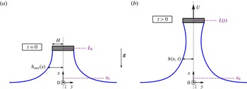
. As pictured in figure 1, the fibre is parallel to the
 $z$
-axis and invariant by translation along this axis. It is supposed to have a rectangular cross-section, of width
 $2H$
, such that the liquid film is pinned at
 $y=\pm H$
. The film is assumed to be symmetric with respect to the vertical
 $x$
-axis, so that only the half-film thickness
 $h(x,t)$
will be considered in the following.
Sketches of the liquid film under consideration, showing the notation and in particular the locations
 $x_{0}$
and
 $L(t)$
where the boundary conditions are imposed. The initial configuration is presented in (a), where a static meniscus connects the fibre, at the initial position
 $L_{0}$
, to the liquid bath located at
 $x=0$
. The configuration in (b) represents the liquid film at a later time, during pulling at a constant velocity
 $U$
.

It is also assumed that the film is uniform in the lateral direction, i.e. perpendicular to the
 $xy$
-plane, such that edge effects are ruled out. During film pulling, the vertical and horizontal velocity fields, respectively denoted
 $u(x,y,t)$
and
 $v(x,y,t)$
and the pressure field
 $P(x,y,t)$
obey the following governing equations and boundary conditions:
-
(i) Navier–Stokes (momentum) equations
(2.1a ) $$\begin{eqnarray}\displaystyle & \displaystyle \unicode[STIX]{x1D70C}(\unicode[STIX]{x2202}_{t}u+u\unicode[STIX]{x2202}_{x}u+v\unicode[STIX]{x2202}_{y}u)=-\unicode[STIX]{x2202}_{x}P+\unicode[STIX]{x1D702}(\unicode[STIX]{x2202}_{xx}u+\unicode[STIX]{x2202}_{yy}u)-\unicode[STIX]{x1D70C}g, & \displaystyle\end{eqnarray}$$
(2.1b )
$$\begin{eqnarray}\displaystyle & \displaystyle \unicode[STIX]{x1D70C}(\unicode[STIX]{x2202}_{t}v+u\unicode[STIX]{x2202}_{x}v+v\unicode[STIX]{x2202}_{y}v)=-\unicode[STIX]{x2202}_{y}P+\unicode[STIX]{x1D702}(\unicode[STIX]{x2202}_{xx}v+\unicode[STIX]{x2202}_{yy}v), & \displaystyle\end{eqnarray}$$
-
(ii) continuity equation
(2.2)
$$\begin{eqnarray}\unicode[STIX]{x2202}_{x}u+\unicode[STIX]{x2202}_{y}v=0,\end{eqnarray}$$
-
(iii) symmetry conditions at
$y=0$
(2.3a )
$$\begin{eqnarray}\displaystyle & \displaystyle v=0, & \displaystyle\end{eqnarray}$$
(2.3b )
$$\begin{eqnarray}\displaystyle & \displaystyle \unicode[STIX]{x2202}_{y}u=0, & \displaystyle\end{eqnarray}$$
-
(iv) kinematic condition at
$y=h(x,t)$
(2.4)
$$\begin{eqnarray}v=\unicode[STIX]{x2202}_{t}h+u\unicode[STIX]{x2202}_{x}h,\end{eqnarray}$$
-
(v) tangential and normal stress balances at
$y=h(x,t)$
in which the continuity equation (2.2) has been used, and where(2.5a )
$$\begin{eqnarray}\displaystyle & \displaystyle \frac{\unicode[STIX]{x1D702}}{1+(\unicode[STIX]{x2202}_{x}h)^{2}}[(1-(\unicode[STIX]{x2202}_{x}h)^{2})(\unicode[STIX]{x2202}_{y}u+\unicode[STIX]{x2202}_{x}v)-4\unicode[STIX]{x2202}_{x}h\unicode[STIX]{x2202}_{x}u]=0, & \displaystyle\end{eqnarray}$$
(2.5b )
$$\begin{eqnarray}\displaystyle & \displaystyle P_{0}-P-\frac{2\unicode[STIX]{x1D702}}{1+(\unicode[STIX]{x2202}_{x}h)^{2}}[(1-(\unicode[STIX]{x2202}_{x}h)^{2})\unicode[STIX]{x2202}_{x}u+\unicode[STIX]{x2202}_{x}h(\unicode[STIX]{x2202}_{y}u+\unicode[STIX]{x2202}_{x}v)]=2\unicode[STIX]{x1D6FE}K, & \displaystyle\end{eqnarray}$$
$P_{0}$
is the atmospheric pressure and
$K$
is the mean curvature of the interface expressed as (2.6)
$$\begin{eqnarray}K(x,t)=\frac{1}{2}\frac{\unicode[STIX]{x2202}_{xx}h}{[1+(\unicode[STIX]{x2202}_{x}h)^{2}]^{3/2}}.\end{eqnarray}$$


The continuity equation (2.2) can then be integrated along the
 $y$
-coordinate, using the Leibniz integral rule and the boundary conditions (2.3a
) and (2.4), such that it yields the mass conservation equation,
 $$\begin{eqnarray}\unicode[STIX]{x2202}_{t}h+\unicode[STIX]{x2202}_{x}(\bar{u}h)=0,\end{eqnarray}$$
where
 $$\begin{eqnarray}\bar{u}(x,t)=\frac{1}{h}\int _{0}^{h}u\,\text{d}y\end{eqnarray}$$
is the average velocity in the film at a given height
 $x$
and time
 $t$
.
2.2 Lubrication approximation and velocity decomposition
We first pose that the characteristic lengths in the
 $x$
- and
 $y$
-directions are, respectively, the capillary length
 $\ell _{c}=\sqrt{\unicode[STIX]{x1D6FE}/\unicode[STIX]{x1D70C}g}$
and the fibre half-width
 $H$
, such that the aspect ratio
 $\unicode[STIX]{x1D700}$
is defined as
 $$\begin{eqnarray}\unicode[STIX]{x1D700}=\frac{H}{\ell _{c}}\ll 1.\end{eqnarray}$$
The smallness of
 $\unicode[STIX]{x1D700}$
corresponds to small space modulations of the dependent variables inherent to the lubrication approximation.
Next, it is well established (see e.g. Howell Reference Howell1996) that when no shear is applied at the interfaces, i.e. the right-hand side of (2.5a
) is zero, the flow at leading order is purely extensional (i.e. a plug flow) and that the vertical velocity is uniform and equal the average velocity
 $\bar{u}$
. Therefore, the vertical velocity field is split into a plug flow contribution
 $\bar{u}(x,t)$
and a shear contribution
 $u_{1}(x,y,t)$
as
 $$\begin{eqnarray}u(x,y,t)=\bar{u}(x,t)+u_{1}(x,y,t),\end{eqnarray}$$
where the dominant contribution
 $\bar{u}$
scales as
 $U$
, while the shear contribution
 $u_{1}(x,y,t)$
is assumed to be of order
 $\unicode[STIX]{x1D700}^{2}U$
. Conservation imposes that
 $$\begin{eqnarray}\int _{0}^{h}u_{1}\,\text{d}y=0.\end{eqnarray}$$
A similar velocity decomposition has been proposed by Schwartz & Roy (Reference Schwartz and Roy1999) aiming at modelling surfactant-stabilised liquid films. For this purpose, they rather imposed a no-slip condition
 $u_{1}(x,h(x,t),t)=0$
for the shear correction, such that the leading-order velocity contribution coincides with the interfacial velocity
 $u_{s}(x,t)$
, instead of
 $\bar{u}(x,t)$
in the present case. The justification of Schwartz and Roy’s approach relies in the fact that
 $u_{s}$
explicitly appears in the transport equation of surfactant at the interface, while such equation is absent in the case of pure liquids.
The continuity equation imposes the horizontal velocity
 $v$
to be of order
 $\unicode[STIX]{x1D700}U$
, the pressure
 $P$
is scaled by
 $\unicode[STIX]{x1D702}\,U/\ell _{c}$
and the time
 $t$
by
 $\ell _{c}/U$
. The system of equations (2.1)–(2.5), in which (2.9) and (2.10) are used, is then non-dimensionlised and truncated at
 $O(\unicode[STIX]{x1D700}^{2})$
. Making the resulting equations dimensional again yields the following approximated system:
-
(i) momentum equations
(2.12a )
$$\begin{eqnarray}\displaystyle & \displaystyle \unicode[STIX]{x1D702}\,\unicode[STIX]{x2202}_{yy}u_{1}=\unicode[STIX]{x2202}_{x}P+\unicode[STIX]{x1D70C}g+\unicode[STIX]{x1D70C}\,(\unicode[STIX]{x2202}_{t}\bar{u}+\bar{u}\unicode[STIX]{x2202}_{x}\bar{u})-\unicode[STIX]{x1D702}\,\unicode[STIX]{x2202}_{xx}\bar{u}, & \displaystyle\end{eqnarray}$$
(2.12b )
$$\begin{eqnarray}\displaystyle & \displaystyle \unicode[STIX]{x2202}_{y}P=0, & \displaystyle\end{eqnarray}$$
-
(ii) continuity equation
(2.13)
$$\begin{eqnarray}\unicode[STIX]{x2202}_{x}\bar{u}+\unicode[STIX]{x2202}_{y}v=0,\end{eqnarray}$$
-
(iii) symmetry conditions at
$y=0$
(2.14a )
$$\begin{eqnarray}\displaystyle & \displaystyle v=0, & \displaystyle\end{eqnarray}$$
(2.14b )
$$\begin{eqnarray}\displaystyle & \displaystyle \unicode[STIX]{x2202}_{y}u_{1}=0, & \displaystyle\end{eqnarray}$$
-
(iv) tangential and normal stress balances at
$y=h(x,t)$
(2.15a )
$$\begin{eqnarray}\displaystyle & \displaystyle \unicode[STIX]{x2202}_{y}u_{1}=4\unicode[STIX]{x2202}_{x}h\,\unicode[STIX]{x2202}_{x}\bar{u}-\unicode[STIX]{x2202}_{x}v, & \displaystyle\end{eqnarray}$$
(2.15b )
$$\begin{eqnarray}\displaystyle & \displaystyle P=P_{0}-2\unicode[STIX]{x1D702}\,\unicode[STIX]{x2202}_{x}\bar{u}-2\unicode[STIX]{x1D6FE}K. & \displaystyle\end{eqnarray}$$


The above system is closed by the unchanged conservation equation (2.7). Note that we did not truncate at
 $O(\unicode[STIX]{x1D700}^{2})$
the expression (2.6) for the mean curvature, despite the higher-order correction at the denominator, as done for liquid bridges by Vincent, Duchemin & Le Dizès (Reference Vincent, Duchemin and Le Dizès2014) for example. This keeps the model compatible with the solution of the static meniscus near the bath, where the slope is not small anymore, and allows describing the entire film shape, from the bath up to the fibre, without having to use a matching procedure between the film region and the static meniscus.
Integrating (2.12b ) leads to a constant pressure in the horizontal direction, whose expression is then given by (2.15b ). In order now to account for van der Waals interactions leading to film rupture, we use the concept of disjoining pressure introduced by Derjaguin & Kusakov (Reference Derjaguin and Kusakov1936). These authors stated that the pressure in a thin film is modified by the molecular interactions as compared with the surrounding bulk phase such that (2.15b ) is rewritten as follows
 $$\begin{eqnarray}P=P_{0}-2\unicode[STIX]{x1D702}\,\unicode[STIX]{x2202}_{x}\bar{u}-2\unicode[STIX]{x1D6FE}K-\unicode[STIX]{x1D6F1},\end{eqnarray}$$
where
 $\unicode[STIX]{x1D6F1}(x,t)$
is the disjoining pressure. Classical theory predicts that the attractive London–van der Waals interaction for a film of thickness
 $2h$
can be expressed as (Israelachvili Reference Israelachvili2011)
 $$\begin{eqnarray}\unicode[STIX]{x1D6F1}(x,t)=-\frac{A_{H}}{6\unicode[STIX]{x03C0}(2h)^{3}},\end{eqnarray}$$
where
 $A_{H}>0$
is the non-retarded Hamaker constant. Note that even though intermolecular forces are bulk contributions, they are equivalently introduced as surface forces in the frame of the lubrication approximation, as thoroughly discussed by Ivanov (Reference Ivanov1988).
Finally, using (2.13) and (2.14a ), the horizontal velocity can be expressed as
 $$\begin{eqnarray}v(x,y,t)=-\unicode[STIX]{x2202}_{x}\bar{u}\,y,\end{eqnarray}$$
and the shear component of the vertical velocity
 $u_{1}$
is obtained by integration of (2.12a
) using (2.11) and (2.14b
),
 $$\begin{eqnarray}u_{1}(x,y,t)=\frac{1}{2\unicode[STIX]{x1D702}}[\unicode[STIX]{x2202}_{x}P+\unicode[STIX]{x1D70C}g+\unicode[STIX]{x1D70C}\,(\unicode[STIX]{x2202}_{t}\bar{u}+\bar{u}\unicode[STIX]{x2202}_{x}\bar{u})-\unicode[STIX]{x1D702}\,\unicode[STIX]{x2202}_{xx}\bar{u}]\left(y^{2}-\frac{h^{2}}{3}\right).\end{eqnarray}$$
Substituting (2.18) and (2.19) into (2.15a ), while using (2.16) and (2.17), finally yields
 $$\begin{eqnarray}\unicode[STIX]{x1D70C}h(\unicode[STIX]{x2202}_{t}\bar{u}+\bar{u}\unicode[STIX]{x2202}_{x}\bar{u})-h\left(2\unicode[STIX]{x1D6FE}\unicode[STIX]{x2202}_{x}K-\unicode[STIX]{x1D70C}g+\frac{A_{H}}{16\unicode[STIX]{x03C0}}\frac{\unicode[STIX]{x2202}_{x}h}{h^{4}}\right)-4\unicode[STIX]{x1D702}\,\unicode[STIX]{x2202}_{x}(h\unicode[STIX]{x2202}_{x}\bar{u})=0.\end{eqnarray}$$
The dimensional system of equations to be solved consists of equations (2.6), (2.7) and (2.20), for the three unknowns,
 $K$
,
 $h$
and
 $\bar{u}$
.
2.3 Non-dimensionalised problem
Applying the following transformations,
 $$\begin{eqnarray}h\rightarrow Hh,\quad x\rightarrow \frac{H}{\unicode[STIX]{x1D700}}x,\quad \bar{u}\rightarrow U\bar{u},\quad t\rightarrow \frac{H}{\unicode[STIX]{x1D700}U}t\quad \text{and}\quad K\rightarrow \frac{\unicode[STIX]{x1D700}^{2}}{H}K,\end{eqnarray}$$
equations (2.7) and (2.20) become in dimensionless form
 $$\begin{eqnarray}\displaystyle & \displaystyle \unicode[STIX]{x2202}_{t}h+\unicode[STIX]{x2202}_{x}(\bar{u}h)=0, & \displaystyle\end{eqnarray}$$
 $$\begin{eqnarray}\displaystyle & \displaystyle We\,h(\unicode[STIX]{x2202}_{t}\bar{u}+\bar{u}\unicode[STIX]{x2202}_{x}\bar{u})-h\left(2\unicode[STIX]{x1D700}\unicode[STIX]{x2202}_{x}K-1+{\mathcal{A}}\,\frac{\unicode[STIX]{x2202}_{x}h}{h^{4}}\right)-4Ca\,\unicode[STIX]{x2202}_{x}(h\unicode[STIX]{x2202}_{x}\bar{u})=0, & \displaystyle\end{eqnarray}$$
 $$\begin{eqnarray}K(x,t)=\frac{\unicode[STIX]{x2202}_{xx}h}{2[1+(\unicode[STIX]{x1D700}\unicode[STIX]{x2202}_{x}h)^{2}]^{3/2}}.\end{eqnarray}$$
In addition to
 $\unicode[STIX]{x1D700}$
, the dimensionless numbers governing the above system of equations are the capillary number, the Weber number and the Hamaker number, respectively defined as
 $$\begin{eqnarray}Ca=\frac{\unicode[STIX]{x1D702}\,U}{\unicode[STIX]{x1D6FE}},\quad We=\frac{\unicode[STIX]{x1D70C}\,U^{2}\ell _{c}}{\unicode[STIX]{x1D6FE}}\quad \text{and}\quad {\mathcal{A}}=\frac{A_{H}\ell _{c}}{16\unicode[STIX]{x03C0}\unicode[STIX]{x1D6FE}H^{3}}.\end{eqnarray}$$
The first two terms in (2.22b ) account for inertia while the others account, respectively, for capillary pressure, gravity, intermolecular forces and extensional viscous stress.
The dimensional physico-chemical parameters we implement in the simulation are those of the V1000 silicone oil that will be used in the experiments presented in § 5, namely
 $\unicode[STIX]{x1D702}=1.00~\text{Pa}~\text{s}$
,
 $\unicode[STIX]{x1D70C}=970~\text{kg}~\text{m}^{-3}$
,
 $\unicode[STIX]{x1D6FE}=21.1~\text{mN}~\text{m}^{-1}$
and
 $A_{H}=4.4\times 10^{-20}~\text{J}$
, yielding a capillary length
 $\ell _{c}=1.49~\text{mm}$
. For a given liquid, the physical parameters that can be changed experimentally are the pulling velocity
 $U$
and the fibre half-width
 $H$
. In the simulation, these parameters will be explored in the ranges
 $0.001~\text{mm}~\text{s}^{-1}\leqslant U\leqslant 30~\text{mm}~\text{s}^{-1}$
and
 $0.1~\unicode[STIX]{x03BC}\text{m}\leqslant H\leqslant 1000~\unicode[STIX]{x03BC}\text{m}$
, respectively. Consequently, the dimensionless numbers defined in (2.24) will vary in the following ranges:
 $$\begin{eqnarray}\displaystyle & \displaystyle 5\times 10^{-5}\leqslant Ca\leqslant 1, & \displaystyle\end{eqnarray}$$
 $$\begin{eqnarray}\displaystyle & \displaystyle 7\times 10^{-11}\leqslant We\leqslant 0.06, & \displaystyle\end{eqnarray}$$
 $$\begin{eqnarray}\displaystyle & \displaystyle 8\times 10^{-14}\leqslant {\mathcal{A}}\leqslant 0.02, & \displaystyle\end{eqnarray}$$
 $$\begin{eqnarray}\displaystyle & \displaystyle 1\times 10^{-4}\leqslant \unicode[STIX]{x1D700}\leqslant 0.6. & \displaystyle\end{eqnarray}$$
 ${\mathcal{A}}$
can be expressed as a function of
 $\unicode[STIX]{x1D700}$
as
 $$\begin{eqnarray}{\mathcal{A}}=\frac{{\mathcal{A}}^{\prime }}{\unicode[STIX]{x1D700}^{3}}\quad \text{where}~{\mathcal{A}}^{\prime }=\frac{A_{H}}{16\unicode[STIX]{x03C0}\unicode[STIX]{x1D6FE}\ell _{c}^{2}}\end{eqnarray}$$
is called the dimensionless Hamaker constant and solely depends on the properties of the liquid. Similarly, the Weber number
 $We$
can be expressed as a function of the capillary number
 $Ca$
and of the liquid properties. Hence, for a given liquid, only
 $Ca$
and
 $\unicode[STIX]{x1D700}$
can be varied independently.
3 Model resolution and validation
3.1 Initial solutions and boundary conditions
We consider the initial configuration pictured in figure 1(a), where the fibre is located at a (dimensionless) position
 $L_{0}$
above the surface of the liquid bath such that it forms a static liquid bridge. Heller (Reference Heller2008) has shown that for
 $L_{0}\leqslant 2$
, a solution exists, whose shape results from a balance between the capillary pressure gradient
 $\unicode[STIX]{x1D6FE}\unicode[STIX]{x2202}_{x}K$
and the hydrostatic pressure gradient
 $\unicode[STIX]{x1D70C}g$
. Integrating the corresponding dimensionless balance
 $$\begin{eqnarray}\unicode[STIX]{x2202}_{x}K_{stat}=\frac{1}{2\unicode[STIX]{x1D700}},\end{eqnarray}$$
with the boundary conditions
 $K_{stat}(0)=0$
,
 $h_{stat}^{\prime }(0)=-\infty$
and
 $h_{stat}(L_{0})=1$
, yields an analytical expression for the shape of the static meniscus,
 $$\begin{eqnarray}h_{stat}(x)=1+\frac{1}{\unicode[STIX]{x1D700}}\left[\sqrt{4-L_{0}^{2}}-\sqrt{4-x^{2}}-\text{arctanh}\left(\frac{2}{\sqrt{4-L_{0}^{2}}}\right)+\text{arctanh}\left(\frac{2}{\sqrt{4-x^{2}}}\right)\right],\end{eqnarray}$$
which is valid in the range
 $0<L_{0}\leqslant 2$
.
The dimensionless initial solutions corresponding to the static meniscus are therefore
 $$\begin{eqnarray}\displaystyle & \displaystyle h(0,x)=h_{stat}(x), & \displaystyle\end{eqnarray}$$
 $$\begin{eqnarray}\displaystyle & \displaystyle K(0,x)=\frac{x}{2\unicode[STIX]{x1D700}}, & \displaystyle\end{eqnarray}$$
 $$\begin{eqnarray}\displaystyle & \displaystyle \bar{u}(0,x)=1/h_{stat}(x), & \displaystyle\end{eqnarray}$$
 $\bar{u}$
using the value resulting from (2.22a
) in stationary regime.
At first sight, the system of equations (2.22)–(2.23) should require five boundary conditions: two on the thickness
 $h$
, two on the vertical velocity
 $\bar{u}$
and one on the mean curvature
 $K$
. However, the order of differentiation on
 $\bar{u}$
can by reduced by one by defining
 $\unicode[STIX]{x1D706}=\unicode[STIX]{x2202}_{x}h$
as an intermediate variable. Using the mass conservation
 $h\unicode[STIX]{x2202}_{x}\bar{u}=-\unicode[STIX]{x2202}_{t}h-\bar{u}\unicode[STIX]{x1D706}$
in equation (2.22b
), only first-order spatial derivative for the variables
 $h$
,
 $\unicode[STIX]{x1D706}$
,
 $K$
and
 $\bar{u}$
are left in the system. The four necessary boundary conditions are then imposed as follows.
A position
 $x_{0}$
is fixed in the static meniscus, close to the surface of the liquid bath
 $x=0$
such that
 $0<x_{0}<L_{0}$
, as sketched in figure 1. The following dimensionless boundary conditions are set at that location:
 $$\begin{eqnarray}\displaystyle & \displaystyle \unicode[STIX]{x2202}_{x}h(t,x_{0})=h_{stat}^{\prime }(x_{0}), & \displaystyle\end{eqnarray}$$
 $$\begin{eqnarray}\displaystyle & \displaystyle K(t,x_{0})=\frac{x_{0}}{2\unicode[STIX]{x1D700}}, & \displaystyle\end{eqnarray}$$
 $x$
-coordinate. The remaining boundary conditions are imposed on the fibre, moving upwards at a constant velocity
 $U$
, and thus located at the dimensionless position
 $L(t)=L_{0}+t$
:
 $$\begin{eqnarray}\displaystyle & \displaystyle h(t,L(t))=1, & \displaystyle\end{eqnarray}$$
 $$\begin{eqnarray}\displaystyle & \displaystyle \bar{u}(t,L(t))=1. & \displaystyle\end{eqnarray}$$
 $x_{0}$
taken in the static meniscus and do not vary significantly with the initial position
 $L_{0}$
of the fibre, as long as
 $L_{0}\leqslant \sqrt{2}$
. These parameters will henceforth be set to
 $x_{0}=0.1$
and
 $L_{0}=\sqrt{2}$
, as justified in appendix A.
The system of partial differential equations (2.22)–(2.23), supplemented by the initial solutions (3.3) and boundary conditions (3.4)–(3.5), is solved using the direct solver MUMPS in COMSOL 5.2. Since the problem involves a moving boundary, the fibre which is lifted at a constant velocity to create the film, the domain geometry is changing with time. The mesh is thus deformed as computed using the arbitrary Lagrangian Eulerian (ALE) algorithm.
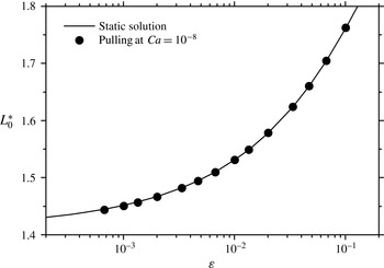
The dimensionless break-up height
 $L_{0}^{\ast }$
of a static film, deduced from (3.6), is plotted as a function of the aspect ratio
 $\unicode[STIX]{x1D700}=H/\ell _{c}$
(solid line). The points correspond to the break-up height computed from our model when pulling at a capillary number
 $Ca=10^{-8}$
, i.e. in a quasi-static regime. The corresponding Weber number is
 $We\approx 3\times 10^{-18}$
and the Hamaker constant is set to
 $A_{H}=4.4\times 10^{-20}~\text{J}$
.

3.2 Static limit
We first check that the static limit is recovered for very small values of
 $Ca$
in (2.22). Thanks to the analytical expression of the thickness profile (3.2) in the static case, it can be shown (Heller Reference Heller2008) that the point of minimal thickness in the static film is located at
 $x=\sqrt{2}$
for
 $\sqrt{2}<L_{0}\leqslant 2$
. The (dimensionless) maximum height
 $L_{0}^{\ast }$
of a static film is then given by
 $h_{stat}(\sqrt{2})=0$
, hence the implicit analytical expression for
 $L_{0}^{\ast }$
:
 $$\begin{eqnarray}\unicode[STIX]{x1D700}=\sqrt{2}-\sqrt{4-(L_{0}^{\ast })^{2}}-\text{arctanh}(\sqrt{2})+\text{arctanh}\left(\frac{2}{\sqrt{4-(L_{0}^{\ast })^{2}}}\right).\end{eqnarray}$$
In figure 2, we compare the maximum height
 $L_{0}^{\ast }$
of a static film given by (3.6) to the break-up height of a quasi-static film pulled at
 $Ca=10^{-8}$
using our model, for different fibre half-widths, i.e. different values of
 $\unicode[STIX]{x1D700}$
. The static limit is successfully recovered in our simulation.
3.3 Comparison with the two-dimensional case
We now compare the results of our lubrication model in the dynamic regime with those reported in Heller (Reference Heller2008), who computed the Stokes equations in a two-dimensional and deformable domain. Note that both inertia and van der Waals forces were neglected in Heller’s simulation, so we temporarily set
 $We=0$
and
 ${\mathcal{A}}=0$
in (2.22) for the sake of consistency.
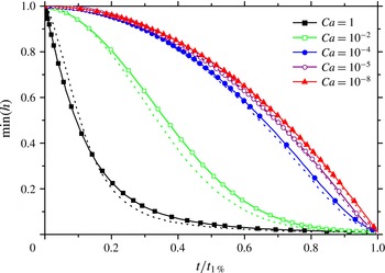
Figure 3 compares the drainage dynamics of films pulled at various velocities for a fixed aspect ratio
 $\unicode[STIX]{x1D700}=0.01$
, using our model (solid lines with symbols) and the two-dimensional simulation results of Heller (Reference Heller2008) (dotted lines). The minimum of the film thickness
 $\text{min}(h)$
is plotted as a function of time, normalised by the time
 $t_{1\,\%}$
when the minimal thickness reaches 0.01, namely 1 % of its initial value. This normalisation allows us to compare the drainage dynamics obtained for different values of the capillary number.
The minimum film thickness
 $\text{min}(h)$
is represented as a function of time
 $t$
, normalised by the time
 $t_{1\,\%}$
when
 $\text{min}(h)$
reaches 1 % of its initial value. For a given capillary number, the solid line with symbols is the drainage curve obtained from our lubrication approach, while the dotted line is the prediction of the two-dimensional simulations reported by Heller (Reference Heller2008). In both cases, the aspect ratio is fixed to
 $\unicode[STIX]{x1D700}=0.01$
and inertia and van der Waals forces are omitted (
 $We=0$
and
 $A_{H}=0$
).

The comparison presented in figure 3 shows that the lubrication approach is in good agreement with the corresponding two-dimensional simulations, especially at small capillary numbers
 $Ca\leqslant 10^{-4}$
. A small discrepancy (less than 10 %) is observed at capillary numbers
 $Ca\geqslant 10^{-2}$
, where the lubrication approximation predicts a slightly slower drainage than the two-dimensional simulations, but the overall shape of the drainage curve is preserved.
4 Results of the model
In this section, we present the numerical results obtained when solving the model described in § 2. In particular, we show that film rupture is a well-defined event, both in space and time. This allows us to introduce the critical thickness for rupture and the film lifetime (or equivalently the film break-up height), which we determine as functions of the aspect ratio
 $\unicode[STIX]{x1D700}$
, the capillary number
 $Ca$
and the dimensionless Hamaker constant
 ${\mathcal{A}}^{\prime }$
.
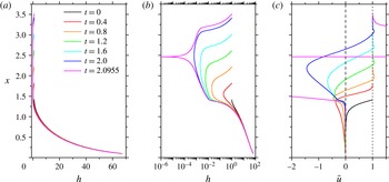
Dimensionless thickness profiles
 $h(x)$
in (a) linear and (b) log scales and (c) average velocity profiles
 $\bar{u}(x)$
at different times during film pulling. These profiles have been obtained by solving the model described in § 2 with a pulling velocity
 $U=1~\text{mm}~\text{s}^{-1}$
(
 $Ca=0.047$
), a fibre half-width
 $H=50~\unicode[STIX]{x03BC}\text{m}$
(
 $\unicode[STIX]{x1D700}=0.034$
) and a Hamaker constant
 $A_{H}=4.4\times 10^{-20}~\text{J}$
. The film rupture, defined as the time when the minimum dimensionless film thickness reaches
 $10^{-6}$
, occurs at
 $t=2.0955$
, corresponding in this case to approximately
 $3$
s. The vertical dotted line at
 $\bar{u}=1$
corresponds to a (dimensional) average velocity equal to the pulling velocity
 $U$
, while the dashed line represents
 $\bar{u}=0$
.

4.1 Thickness and velocity profiles
Typical film thickness profiles
 $h(x)$
are represented in figure 4 in (a) linear and (b) log scales, at different times during pulling. At
 $t=0$
, a static meniscus spans between the liquid bath at
 $x=0$
and the fibre, which is initially located at
 $L_{0}=\sqrt{2}$
and set into motion at a constant velocity
 $U$
(
 $U=1~\text{mm}~\text{s}^{-1}$
in figure 4). As the fibre goes up, the liquid film grows in height and thins, as shown in figure 4(a,b). Once the film has become sufficiently thin, the van der Waals term
 ${\mathcal{A}}\,\unicode[STIX]{x2202}_{x}h/h^{3}$
comes into play in (2.22b
), as we will see in a more quantitative way in § 4.3. This term ultimately triggers the film break-up, which is characterised by a very rapid and localised drop of the film thickness, as demonstrated by the magenta curve at
 $t=2.0955$
in figure 4(b).
Figure 4(c) displays the spatial variation of the average velocity
 $\bar{u}$
in the film at different times during film pulling, for the same parameters as in figure 4(a,b). The initial velocity profile (black curve) differs slightly from the initial condition (3.3c
) and is numerically converged towards at time
 $t=0$
to satisfy (2.22)–(2.23). For
 $t>0.4$
, the velocity in the static meniscus (
 $x\lesssim \sqrt{2}$
) goes back to zero and the initial velocity profile is forgotten. At all times
 $t>0$
, the average velocity
 $\bar{u}$
is negative in the lower part of the film and positive in its upper part. Consequently, there is a location in the film where
 $\bar{u}=0$
, which is close to the minimum in the thickness profile. The liquid is expelled from this minimum with a flow rate that seems to diverge at the point of rupture (magenta curve, at
 $t=2.0955$
). The flow in the vicinity of the point of minimal thickness is further studied in appendix B, where the streamlines are computed for various times during film pulling.
The minimum thickness
 $\text{min}(h)$
is plotted as a function of time in dimensionless units, for various values of the pulling velocity
 $U$
(solid lines) and a fixed fibre half-width
 $H=50~\unicode[STIX]{x03BC}\text{m}$
(
 $\unicode[STIX]{x1D700}=0.034$
) and Hamaker constant
 $A_{H}=4.4\times 10^{-20}~\text{J}$
. For
 $U\gtrsim 0.2~\text{mm}~\text{s}^{-1}$
(
 $Ca\gtrsim 0.01$
), a ‘slow’ drainage regime is first observed, followed by a sharp decrease in thickness, corresponding to film rupture. The transition from the drainage to the rupture regime happens when the film reaches a critical thickness, which can be defined as the intersection between a power-law fit of the end of the drainage regime (dashed line) and the rupture regime (dotted lines).

4.2 Film drainage and rupture
We now follow the film thickness at the point where it is minimal as a function of time. The thinning dynamics at this point is displayed in figure 5 (solid lines) for different values of the pulling velocity
 $U$
. For velocities above
 $0.1~\text{mm}~\text{s}^{-1}$
, the thinning dynamics exhibits two distinct parts: a drainage regime, where the thickness gently decreases with time, and a rupture regime, where the thickness drops abruptly.
In practice, the simulation is stopped when the minimal thickness
 $\text{min}(h)$
reaches
 $10^{-6}$
, which corresponds to a subangstrom film thickness for the example displayed in figure 4 (where
 $H=50~\unicode[STIX]{x03BC}\text{m}$
). The dimensionless film lifetime
 $\unicode[STIX]{x1D70F}$
is then defined as the time when
 $\text{min}(h)=10^{-6}$
and the corresponding dimensionless break-up height is given by
 $L^{\ast }=L_{0}+\unicode[STIX]{x1D70F}=\sqrt{2}+\unicode[STIX]{x1D70F}$
. Note that this definition does not depend on the cutoff value
 $10^{-6}$
as long as the rupture regime, where the slope is almost vertical, has been reached. Thus, the break-up height of the film is an observable, which will be studied in details in § 4.4. Note that the model also gives a prediction for the location of the puncture in the film, which we compare with experimental observations in appendix C.
The dimensionless (respectively dimensional) critical thickness for rupture
 $h^{\ast }$
(respectively
 $H\times h^{\ast }$
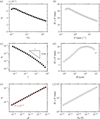
) is plotted as a function of the control parameters, one being varied at a time with the others fixed to the following values:
 $\unicode[STIX]{x1D700}=0.034$
(
 $H=50~\unicode[STIX]{x03BC}\text{m}$
),
 $Ca=0.47$
(
 $U=10~\text{mm}~\text{s}^{-1}$
) and
 ${\mathcal{A}}^{\prime }=A_{H}/16\unicode[STIX]{x03C0}\unicode[STIX]{x1D6FE}\ell _{c}^{2}=1.84\times 10^{-14}$
(
 $A_{H}=4.4\times 10^{-20}~\text{J}$
).

4.3 Critical thickness for rupture
The transition from the drainage regime to the rupture regime in figure 5 occurs around a critical film thickness, when the van der Waals forces come into play. We define this critical thickness for rupture, denoted
 $h^{\ast }$
, as the intersection between a power-law fit of the end of the drainage regime (dashed line in figure 5) and the rupture regime (dotted lines in figure 5). The variation of the critical thickness
 $h^{\ast }$
with the capillary number
 $Ca$
, the aspect ratio
 $\unicode[STIX]{x1D700}$
and the dimensionless Hamaker constant
 ${\mathcal{A}}^{\prime }=A_{H}/16\unicode[STIX]{x03C0}\unicode[STIX]{x1D6FE}\ell _{c}^{2}$
are respectively displayed in figure 6(a,c,e). The dimensional counterparts of these data sets are shown in figure 6(b,d,f), where the dimensional critical thickness
 $H\times h^{\ast }$
is plotted as a function of the pulling velocity
 $U$
, the fibre half-width
 $H$
and the Hamaker constant
 $A_{H}$
.
Figure 6(a,b) show that the critical thickness
 $h^{\ast }$
decreases with the pulling velocity for capillary numbers in the range
 $0.01\lesssim Ca\lesssim 1$
where the drainage and rupture regimes are clearly distinguished (see figure 5). For
 $Ca\lesssim 0.01$
, the critical thickness is no longer defined in our approach since the drainage and rupture regimes merge. The decrease of
 $h^{\ast }$
with
 $Ca$
shows that entrainment is a stabilising factor for the film, in the sense that the destabilising effect of van der Waals forces is delayed, i.e. comes into play for thinner films.
Figure 6(c) indicates that the critical thickness also decreases with the aspect ratio
 $\unicode[STIX]{x1D700}$
. This behaviour can be qualitatively understood from the fact that the scale of the van der Waals contribution in (2.22b
) is set by the Hamaker number
 ${\mathcal{A}}={\mathcal{A}}^{\prime }/\unicode[STIX]{x1D700}^{3}$
. For a given dimensionless Hamaker constant
 ${\mathcal{A}}^{\prime }$
, the larger the aspect ratio, the smaller the Hamaker number and so the smaller the thickness required for
 ${\mathcal{A}}\,\unicode[STIX]{x2202}_{x}h/h^{4}$
to be of leading order, hence the decrease of
 $h^{\ast }$
with
 $\unicode[STIX]{x1D700}$
. More quantitatively, the variation of the critical thickness compares favourably with the power law
 $h^{\ast }\propto \unicode[STIX]{x1D700}^{-0.96}$
for
 $\unicode[STIX]{x1D700}=10^{-2}{-}10^{-1}$
, as will be justified later. The critical thickness varies more slowly than
 $\unicode[STIX]{x1D700}^{-1}$
below
 $\unicode[STIX]{x1D700}\sim 10^{-1}$
, but faster than
 $\unicode[STIX]{x1D700}^{-1}$
for
 $\unicode[STIX]{x1D700}\gtrsim 10^{-1}$
, hence the non-monotonic behaviour of the dimensional critical thickness
 $H\times h^{\ast }$
as a function of the fibre half-width
 $H$
, as shown in figure 6(d). This change in behaviour for
 $\unicode[STIX]{x1D700}\gtrsim 10^{-1}$
is likely due to the
 $\unicode[STIX]{x1D700}^{2}$
term in the denominator of the mean curvature (2.23), which becomes non-negligible.
Finally, figure 6(e,f) display the variation of the critical thickness with the dimensionless Hamaker constant
 ${\mathcal{A}}^{\prime }=A_{H}/16\unicode[STIX]{x03C0}\unicode[STIX]{x1D6FE}\ell _{c}^{2}$
, which is a property of the liquid. The parameters
 $Ca$
and
 $\unicode[STIX]{x1D700}$
remain fixed, while the Hamaker constant
 $A_{H}$
is varied in the range
 $10^{-22}{-}10^{-18}~\text{J}$
, all the other properties of the liquid being set to the values given in § 2.3. The critical thickness
 $h^{\ast }$
increases with the dimensionless Hamaker constant as a power law (solid line in figure 6
e) with an exponent
 $\unicode[STIX]{x1D6FC}\approx 0.32$
.
Such a power-law behaviour for the critical thickness as a function of the Hamaker constant had already been predicted by Vrij & Overbeek (Reference Vrij and Overbeek1968) for small horizontal liquid films. Their approach consisted in calculating the film lifetime by summing the time needed for the film to reach a certain thickness and the time required for a van der Waals-driven instability to develop. Under the assumption of flat and rigid liquid/air interfaces, they derived the critical thickness, which was found to vary with the Hamaker constant as
 $A_{H}^{2/7}$
(
 $2/7\approx 0.29$
), an exponent which is close to our value of 0.32. The difference probably stems from the flow in our continuously stretched film with stress-free interfaces, which is quite different from the Poiseuille flow expected for rigid interfaces.
We finally give arguments regarding how the power-law behaviour of the critical thickness
 $h^{\ast }$
versus
 ${\mathcal{A}}^{\prime }$
can be related to the variation of
 $h^{\ast }$
with
 $\unicode[STIX]{x1D700}$
. Figure 6(e) shows that the critical thickness follows
 $h^{\ast }=\unicode[STIX]{x1D6FD}{{\mathcal{A}}^{\prime }}^{\unicode[STIX]{x1D6FC}}$
, where
 $\unicode[STIX]{x1D6FC}$
and
 $\unicode[STIX]{x1D6FD}$
are a priori functions of
 $\unicode[STIX]{x1D700}$
and
 $Ca$
(for example,
 $\unicode[STIX]{x1D6FC}=0.32$
for
 $\unicode[STIX]{x1D700}=0.034$
and
 $Ca=0.47$
). Considering that film rupture is essentially driven by the Hamaker number
 ${\mathcal{A}}={\mathcal{A}}^{\prime }/\unicode[STIX]{x1D700}^{3}$
, we can assume that, for a given capillary number
 $Ca$
, the critical thickness
 $h^{\ast }$
is essentially a function of
 ${\mathcal{A}}$
:
 $h^{\ast }=f({\mathcal{A}})$
. Still for a fixed capillary number, this is equivalent to saying that
 $h^{\ast }$
depends on
 $\unicode[STIX]{x1D700}$
only through
 ${\mathcal{A}}={\mathcal{A}}^{\prime }/\unicode[STIX]{x1D700}^{3}$
, i.e.
 $h^{\ast }=f({\mathcal{A}})=f({\mathcal{A}}^{\prime }/\unicode[STIX]{x1D700}^{3})=\unicode[STIX]{x1D6FD}(\unicode[STIX]{x1D700})\times {{\mathcal{A}}^{\prime }}^{\unicode[STIX]{x1D6FC}(\unicode[STIX]{x1D700})}$
. This imposes that the exponent
 $\unicode[STIX]{x1D6FC}$
is independent of
 $\unicode[STIX]{x1D700}$
and that
 $\unicode[STIX]{x1D6FD}(\unicode[STIX]{x1D700})\propto \unicode[STIX]{x1D700}^{-3\unicode[STIX]{x1D6FC}}$
, i.e.
 $h^{\ast }\propto \unicode[STIX]{x1D700}^{-0.96}$
for
 $Ca=0.47$
and
 ${\mathcal{A}}^{\prime }=1.84\times 10^{-14}$
. Figure 6(c) shows that the assumption that
 $h^{\ast }=f({\mathcal{A}})$
seems reasonable, but is not rigorously true for
 $\unicode[STIX]{x1D700}\lesssim 0.01$
and
 $\unicode[STIX]{x1D700}\gtrsim 0.1$
, since the data deviate from the
 $h^{\ast }\propto \unicode[STIX]{x1D700}^{-0.96}$
behaviour.
The variations of the critical thickness with
 $Ca$
and
 $\unicode[STIX]{x1D700}$
point to the fact that
 $h^{\ast }$
is not an intrinsic property of the liquid but also depends on the experimental conditions and flow dynamics. Numerous studies (see e.g. Manev & Nguyen Reference Manev and Nguyen2005) have been dedicated to the critical thickness of horizontal thin liquid films, from both the experimental and theoretical point of view. The results presented in figure 6(b,d) put into question the applicability of these static investigations to dynamic situations, such as foam generation for instance.
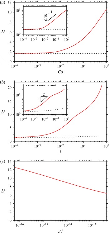
The dimensionless film break-up height
 $L^{\ast }$
is plotted (a) as a function of the capillary number
 $Ca$
for a fixed fibre half-width
 $H=50~\unicode[STIX]{x03BC}\text{m}$
(
 $\unicode[STIX]{x1D700}=0.034$
) in log-linear and log-log scale (inset), (b) as a function of the aspect ratio
 $\unicode[STIX]{x1D700}$
for a fixed pulling velocity
 $U=10~\text{mm}~\text{s}^{-1}$
(
 $Ca=0.47$
) in log-linear and log-log scale (inset), and (c) as a function of the dimensionless Hamaker constant
 ${\mathcal{A}}^{\prime }=A_{H}/16\unicode[STIX]{x03C0}\unicode[STIX]{x1D6FE}\ell _{c}^{2}$
for
 $H=50~\unicode[STIX]{x03BC}\text{m}$
and
 $U=10~\text{mm}~\text{s}^{-1}$
. The dotted lines represent the static limit given by (3.6).

4.4 Maximal height of the film
As demonstrated in §§ 4.1 and 4.2, the height
 $L^{\ast }$
reached by the film when the rupture occurs is well defined. In figure 7, we report this break-up height as a function of the capillary number
 $Ca$
(figure 7
a) and the aspect ratio
 $\unicode[STIX]{x1D700}$
(figure 7
b) for given liquid properties. For fixed pulling parameters, the effect of the dimensionless Hamaker constant
 ${\mathcal{A}}^{\prime }$
on the break-up height
 $L^{\ast }$
is displayed in figure 7(c).
For
 $Ca\lesssim 10^{-3}$
, the break-up height of the film is equal to the static limit given by (3.6) (dotted line in figure 7
a). Beyond this value,
 $L^{\ast }$
increases with the capillary number, which is expected since the creation of the film is driven by viscous entrainement. This increase approximately follows a power law of exponent 0.38, as shown in the inset of figure 7(a). Note that, for given liquid properties, the value of the exponent may a priori depend on the aspect ratio
 $\unicode[STIX]{x1D700}$
.
As displayed in figure 7(b), the break-up height
 $L^{\ast }$
is also an increasing function of the aspect ratio. This can be understood from the fact that the larger the aspect ratio
 $\unicode[STIX]{x1D700}$
, the smaller the Hamaker number
 ${\mathcal{A}}={\mathcal{A}}^{\prime }/\unicode[STIX]{x1D700}^{3}$
and the thinner the film when van der Waals forces come into play and trigger film rupture. The
 $\unicode[STIX]{x1D700}$
dependency of the break-up height seems to exhibit three different regimes. For
 $\unicode[STIX]{x1D700}\lesssim 10^{-3}$
, the static limit given by (3.6) (dotted line in figure 7
b) is asymptotically reached. As shown in the inset in figure 7(b), the break-up height
 $L^{\ast }$
then appears to follow a power-law increase of exponent
 $1/2$
up to
 $\unicode[STIX]{x1D700}\sim 3\times 10^{-2}$
. Beyond, it enters a third regime where the break-up height rises more slowly than
 $\unicode[STIX]{x1D700}^{1/2}$
. This is likely again a signature of the
 $\unicode[STIX]{x1D700}^{2}$
term in the denominator of the mean curvature (2.23), which becomes non-negligible for
 $\unicode[STIX]{x1D700}\gtrsim 10^{-1}$
.
Finally, the film break-up height decreases with the dimensionless Hamaker constant, due to the contribution of
 ${\mathcal{A}}^{\prime }$
to the Hamaker number
 ${\mathcal{A}}$
. The break-up height turns out to be less sensitive to the Hamaker constant, varied in the range
 $A_{H}=10^{-22}{-}10^{-18}~\text{J}$
, than to the fibre half-width
 $H$
or to the pulling velocity
 $U$
.
Note that solving the system without inertia, i.e. setting
 $We=0$
in equation (2.22b
), essentially yields the same results. Although it plays virtually no part within the range of parameters explored here, inertia was kept in all simulations since it was found to help the convergence of the numerical solver used in COMSOL.
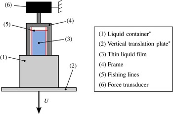
Sketch of the experimental set-up used to measure the maximal height of vertical liquid films. A container (1) filled with liquid is bound to a vertical motorised translation plate (2). By lowering the container at a constant velocity
 $U$
, a thin liquid film (3) is deposited on a fixed frame (4) gridded with fishing lines (5). The break-up of this film is detected using the force transducer (6) to which the frame is attached. The stars indicate the elements of the set-up which are mobile in the reference frame of the laboratory.

5 Experiments: materials and methods
In the following, we measure experimentally the break-up height of pure liquid films in order to test the predictions of the model presented in § 4. More specifically, we investigate the influence of the capillary number
 $Ca$
by varying the pulling velocity
 $U$
and the liquid viscosity
 $\unicode[STIX]{x1D702}$
, and the influence of the aspect ratio
 $\unicode[STIX]{x1D700}$
by using different fibre diameters.
5.1 Experimental set-up and protocol
The liquid films are formed on a
 $2~\text{cm}\times 9~\text{cm}$
rigid acrylonitrile butadiene styrene (ABS) frame covered in cross-linked polyepoxide to avoid liquid penetration. As sketched in figure 8, the frame is gridded with one horizontal and two vertical nylon fishing lines of diameter
 $D=11$
, 57 or
 $175~\unicode[STIX]{x03BC}\text{m}$
. The spacing between the vertical fishing lines is equal to
 $15~\text{mm}$
. The frame is initially immersed in a liquid container, the horizontal fishing line being located at about
 $1~\text{mm}$
below the surface of the liquid bath. While the frame remains fixed during the whole experiment, the liquid container can be lowered at a constant velocity
 $0.01~\text{mm}~\text{s}^{-1}\leqslant U\leqslant 10~\text{mm}~\text{s}^{-1}$
using a motorised linear stage (Newport UTS 150 CC) coupled to a motion controller (Newport SMC 100 CC), hence creating a thin liquid film between the fishing lines.
The film lifetime
 $\unicode[STIX]{x1D70F}_{exp}$
is defined in the experiments as the difference between the time when the horizontal fishing line crosses the surface of the liquid bath and the time when the film breaks. This experimental definition would correspond to an initial meniscus height
 $L_{0,\mathit{dim}}=0$
in the simulations. The film rupture is detected thanks to the force sensor (HBM, 5 g) on which the frame is attached. When the film bursts, the signal measured by the force transducer undergoes a jump due to the disappearance of the surface tension contribution to the total vertical force exerted on the frame. When this jump is detected, the translation plate automatically stops and comes back to its initial position. This automated set-up allows for statistical measurements of the film lifetime
 $\unicode[STIX]{x1D70F}_{exp}$
or, equivalently, of the film break-up height
 $L_{exp}^{\ast }=U\unicode[STIX]{x1D70F}_{exp}$
.
Main physical properties of the silicone oils used in the experiments. The viscosity and surface tension are given at
 $25\,^{\circ }\text{C}$
and have been measured after the fractionation processes for the
 $V350$
and
 $V1000$
oils. The experimental errors are
 ${\lesssim}0.5\,\%$
for viscosity measurements and
 $\pm 0.1~\text{mN}~\text{m}^{-1}$
for surface tension measurements. The number average molar mass
 $M_{n}$
is deduced from the viscosity using the expression
 $\log \unicode[STIX]{x1D702}=1.00+0.0123\,M_{n}^{1/2}$
(Mark Reference Mark1999).

5.2 Finding a pure liquid
In our experiments, the liquid used to form the films is silicone oil (methyl-terminated polydimethylsiloxane, PDMS, purchased from either Sigma Aldrich or Bluestar silicones), which is often considered as a model Newtonian pure liquid. The physicochemical parameters of the different silicone oils tested in the experiments are summed up in table 1. The viscosities and surface tensions were respectively measured with a Physica MCR 300 rheometer and the rising bubble technique (Tracker, TECLIS), in the temperature range
 $T=18{-}25\,^{\circ }\text{C}$
. The Hamaker constant is expected to be the same for all the silicone oils used in this study and equal to
 $A_{H}=4.4\times 10^{-20}~\text{J}$
at
 $20\,^{\circ }\text{C}$
(Drummond & Chan Reference Drummond and Chan1997).
As the liquid viscosity is varied over more than two orders of magnitude, the other physicochemical parameters, i.e. density and surface tension (see table 1) as well as the Hamaker constant, remain virtually constant. This allows us to consider that, for a given pulling velocity
 $U$
and a given fibre half-width
 $H$
, changing the liquid will only affect the viscosity, hence the value of the capillary number
 $Ca$
, while leaving the other dimensionless parameters
 $\unicode[STIX]{x1D700}$
,
 $We$
and
 ${\mathcal{A}}$
unchanged.
The model we have built in § 2 is valid only for pure liquids, i.e. in the absence of tangential stress at the interfaces. The experimental difficulty is that any small surface tension gradient, due to temperature inhomogeneity or surface active agents for example, will invalidate the stress-free boundary condition at the interfaces (2.5a
). Because of their high surface tension, water surfaces are particularly prone to be contaminated by surface active impurities, which can lead to surface tension gradients. It has been shown that the drainage of a water film between two bubbles can be modelled using a no-slip boundary condition for surface tension gradients as small as
 $0.1~\text{mN}~\text{m}^{-2}$
(Yaminsky et al.
Reference Yaminsky, Ohnishi, Vogler and Horn2010). This is the reason why we turned to silicone oil as a model pure liquid in the first place.
Commercially available silicone oils are actually mixtures of PDMS chains of different lengths (or equivalently of different molar masses), the distribution of which is peaked around the number average molar mass
 $M_{n}$
. The surface tension of silicone oil increases with the number average molar mass up to
 $M_{n}\sim 10^{4}~\text{g}~\text{mol}^{-1}$
, where the surface tension saturates at a constant value
 $\unicode[STIX]{x1D6FE}\approx 21~\text{mN}~\text{m}^{-1}$
(Mark Reference Mark1999). Since short PDMS chains (i.e. with a molar mass less than approximately
 $10^{4}~\text{g}~\text{mol}^{-1}$
) have a lower surface tension than longer chains, any spatial heterogeneity in their concentration, either due to the creation of fresh interface or to evaporation, can generate surface tension gradients. This phenomenon was already observed by Bascom, Cottington & Singleterry (Reference Bascom, Cottington and Singleterry1964) to have a strong influence on the spreading of oil on solid surfaces. Similarly, we suspect that traces of short PDMS chains may be sufficient to create interfacial shear stress in our silicone oil films, thus resulting in their overstabilisation.
To avoid this problem, we use a basic fractionation protocol to get rid of the shortest chains in silicone oil. The commercial silicone oil is poured into a separator funnel with about three times as much acetone (in volume). The mixture is vigorously shaken for five minutes and left to decant for several hours. Short PDMS chains are soluble in acetone while longer chains are not, so when the phase separation is complete, the PDMS phase contains less short chains than initially. The PDMS phase is then extracted, left in an oven at
 $60\,^{\circ }\text{C}$
for at least 20 h and finally put in a vacuum chamber for at least 20 h to remove the remaining acetone.
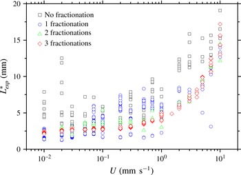
Figure 9 shows the break-up height of
 $V350$
silicone oil films as a function of the pulling velocity for a non-fractionated and (up to three times) fractionated oils. While the data corresponding to the non-fractionated oil are scattered, the application of the fractionation protocol described above yields much more reproducible results. Moreover, fractionated oils lead, on average, to shorter films than the non-fractionated oil, supporting the hypothesis of surface tension gradients due to short PDMS chains. The lower the viscosity, the more short chains in the oil. Thus, the fractionation protocol had to be applied three times to the
 $V350$
oil, but only once to the
 $V1000$
oil to get reproducible results. No fractionation was needed for the most viscous oils (
 $V10000$
,
 $V12500$
and
 $V60000$
).
6 Experiments: results and comparison with theory
6.1 Influence of the pulling velocity
Using a nylon fibre of fixed diameter
 $D=175~\unicode[STIX]{x03BC}\text{m}$
, the influence of the pulling velocity
 $U$
on the film break-up height is first explored for silicone oils of various viscosities. The film break-up height is measured using the protocol described in § 5.1 and the experiment is repeated at least 20 times for a given velocity and a given liquid viscosity. In the results presented in figure 10, each point is thus an average over at least 20 points and the error bar represents the square root of the quadratic sum of the standard deviation and a systematic error of
 $\pm 0.5~\text{mm}$
on the position of the liquid bath surface. It can be noted that the standard deviation of the measurements increases with
 $Ca$
, which may be due to the finite acquisition frequency of the force sensor used to detect film rupture.
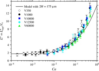
Data points were obtained with pulling velocities varying over three orders of magnitude and liquid viscosities varying over two orders of magnitude. They collapse onto a single master curve when plotted versus the capillary number
 $Ca=\unicode[STIX]{x1D702}\,U/\unicode[STIX]{x1D6FE}$
. Note that the data corresponding to the less viscous oil (
 $V350$
) lie slightly above the others for
 $Ca\gtrsim 0.1$
, perhaps because of residual surface tension gradients due to short PDMS chains that were not removed by the fractionation protocol.
The experimental data are in good agreement with our model with
 $2H=175~\unicode[STIX]{x03BC}\text{m}$
(solid line in figure 10) up to
 $Ca\sim 0.1$
. A small deviation from the theoretical prediction is observed at capillary numbers larger than 0.1, where the films last longer than expected from the model, as will be discussed in § 6.3.
The experimental break-up height
 $L_{exp}^{\ast }$
of
 $V350$
silicone oil films is measured as a function of the pulling velocity
 $U$
with a nylon fibre of diameter
 $D=175~\unicode[STIX]{x03BC}\text{m}$
. The various symbols/colours show the data obtained after the application of
 $n$
fractionations (
 $0\leqslant n\leqslant 3$
) to the silicone oil taken from the bottle. The fractionation protocol, which aims at removing the shortest methyl-terminated polydimethylsiloxane chains, significantly improves the reproducibility of the measurements.

The break-up height
 $L_{exp}^{\ast }$
of films made from silicone oils of various viscosities is measured as a function of the pulling velocity
 $U$
, using the same nylon fibre of diameter
 $D=175~\unicode[STIX]{x03BC}\text{m}$
. The film break-up height is non-dimensionalised by the capillary length
 $\ell _{c}=1.49~\text{mm}$
and displayed as a function of the capillary number
 $Ca=\unicode[STIX]{x1D702}\,U/\unicode[STIX]{x1D6FE}$
. The non-dimensionalised experimental data (symbols) collapse onto a single master curve, which is compared to the prediction of our model (solid line, see also figure 7
a) with
 $2H=175~\unicode[STIX]{x03BC}\text{m}$
.

The break-up height
 $L_{exp}^{\ast }$
of films made from silicone oil is measured as a function of the pulling velocity
 $U$
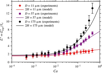
, using nylon fibres of various diameters. The experimental data (symbols) are non-dimensionalised as in figure 10 and compared with the predictions of our model (solid lines), where
 $2H$
has been set equal to the fibre diameter
 $D$
. The data for
 $D=11$
and
 $175~\unicode[STIX]{x03BC}\text{m}$
were obtained using the
 $V1000$
silicone oil, while the experiments for
 $D=57~\unicode[STIX]{x03BC}\text{m}$
were carried out with the
 $V10000$
silicone oil.

6.2 Influence of the fibre diameter
The effect of the diameter
 $D$
of the horizontal fibre which supports the film is then investigated experimentally. The film break-up height is measured as a function of the capillary number for three different fibre diameters,
 $D=11$
, 57 and
 $175~\unicode[STIX]{x03BC}\text{m}$
and the results are shown in figure 11. As in figure 10, each data point is averaged over at least 20 measurements. The theoretical predictions computed from our model, setting
 $2H=11$
, 57 and
 $175~\unicode[STIX]{x03BC}\text{m}$
(i.e.
 $\unicode[STIX]{x1D700}=0.0037$
, 0.019 and 0.059, respectively), are also displayed in figure 11.
For all fibre diameters, the experimental data are in good agreement with the theoretical predictions for
 $Ca\leqslant 0.1$
. The deviation previously observed at higher capillary numbers for the thickest fibre (
 $D=175~\unicode[STIX]{x03BC}\text{m}$
) is reduced as the fibre diameter diminishes and the data for the thinnest fibres (
 $D=57~\unicode[STIX]{x03BC}\text{m}$
and
 $D=11~\unicode[STIX]{x03BC}\text{m}$
) stay in line with the model for the whole range of capillary numbers probed in the experiments.
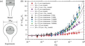
(a) Sketches of the boundary condition at the fibre in the model (top), assuming a rectangular cross-section of width
 $2H$
, and in the experiments (bottom), where the fibre has a circular cross-section of diameter
 $D$
, certainly coated with a liquid layer, leading to an effective fibre width
 $2H_{eff}>D$
. (b) The sets of experimental data displayed in figures 10 and 11 are replotted together (symbols) and compared with the predictions of the model (dashed lines) using an effective fibre
 $2H_{eff}=D+2h_{LL}$
to account for the coating of a liquid layer of thickness
 $h_{LL}$
around the fibre. The solid lines are again the predictions of the model assuming
 $2H=D$
.

6.3 Discussion
The simulations are in quantitative agreement with the experimental data, except at capillary numbers
 $Ca\gtrsim 0.1$
, where the maximal film length is actually underestimated by the simulations. Several hypotheses can be proposed to explain this discrepancy. First, we showed that the results of the full two-dimensional approach (Heller Reference Heller2008) are successfully recovered by our lubrication model for
 $Ca<10^{-2}$
, but that a small deviation appears for larger capillary numbers (see figure 3). The difference between our model and the experimental break-up height observed for
 $Ca\gtrsim 0.1$
may then be attributed to two-dimensional effects that are not captured in our lubrication analysis.
Since the deviation from the theoretical prediction depends on the fibre diameter, we may also seek its explanation in the boundary condition at the top of the film, where it meets the supporting fibre. In the model, we impose that the thickness
 $2h$
at the top of the film is equal to the width
 $2H$
of the fibre. To compute the solid lines in figures 10 and 11, we assumed that
 $2H$
is equal to the diameter
 $D$
of the nylon fishing line used in the experiments. However, in practice, we can expect the nylon fibre to be coated with a liquid layer as it crosses the surface of the liquid pool, thus corresponding to an effective boundary condition with
 $2H_{eff}>D$
, as pictured in figure 12(a). Since the film break-up height
 $L^{\ast }$
is an increasing function of
 $\unicode[STIX]{x1D700}$
, i.e. of
 $H$
, see figure 7(b), the underestimation of
 $H$
can lead to an underestimation of
 $L^{\ast }$
.
In order to get a more quantitative insight into the effect of fibre coating on the film break-up height, we need to estimate the thickness of the liquid layer coated onto the horizontal fibre as it crosses the interface. This is actually a complex time-dependent problem, which is however related to the classical problem of vertical fibre coating. The latter was solved in stationary regime by Landau & Levich (Reference Landau and Levich1942), who found an entrained thickness
 $h_{LL}$
proportional to
 $Ca^{2/3}$
. Assuming that
 $h_{LL}$
gives the correct order of magnitude for the thickness of the liquid layer coated onto a horizontal fibre, we have solved our model (§ 2) where
 $2H$
was replaced by the effective value
 $$\begin{eqnarray}2H_{eff}(Ca)=D+2h_{LL}(Ca)=D(1+1.34\,Ca^{2/3}).\end{eqnarray}$$
The corresponding predictions are displayed as dashed lines in figure 12(b), along with the experimental data of figures 10 and 11 (symbols), and with the predictions of the model assuming
 $2H=D$
(solid lines, same as in figure 11). As expected from equation (6.1), the influence of the coated layer becomes significant only for
 $Ca\gtrsim 0.1$
. It leads to a better agreement between the model’s prediction and the experimental data for the thickest fibre (
 $D=175~\unicode[STIX]{x03BC}\text{m}$
), but to an overestimation of the film break-up height for the thinnest fibres (
 $D=11~\unicode[STIX]{x03BC}\text{m}$
and
 $D=57~\unicode[STIX]{x03BC}\text{m}$
).
This overestimation of the break-up height is not particularly surprising since our way of taking into account the coated liquid layer is quite crude. The coated layer is not simply static during film pulling but can also drain by capillarity with a typical time scale
 $\unicode[STIX]{x1D702}D/2\unicode[STIX]{x1D6FE}$
(Kočárková et al.
Reference Kočárková, Rouyer and Pigeonneau2013), which is at most
 $0.3$
s for the thickest fibre (
 $D=175~\unicode[STIX]{x03BC}\text{m}$
) and the most viscous oil (
 $V60000$
). This drainage time is always much shorter than the experimental film lifetime, which lies in the range
 $\unicode[STIX]{x1D70F}\sim 2{-}240$
s, depending on the pulling velocity. The liquid layer coated onto the fibre may then feed the film and thus delay its rupture in a way which is not straightforward to estimate. Finally, the above arguments show that the discrepancy between the presented model and the experiments at high capillary number may be explained by fibre coating. However, taking this effect into account in the simulation a more quantitative way would require the development of a model for horizontal fibre coating and thus lies beyond the scope of this paper.
7 Conclusions
In this article, we described the pulling of a liquid film with stress-free interfaces by the means of a non-stationary model in the lubrication approximation. The entire life of the film could be addressed, from an initial static meniscus bridging the gap between a horizontal fibre and a liquid pool, until film rupture under the action of van der Waals forces. The film rupture turned out to be well defined by a swift and localised decrease of the film thickness, allowing the definition of the critical thickness for rupture
 $h^{\ast }$
for capillary numbers
 $Ca\gtrsim 0.01$
and of the film break-up height
 $L^{\ast }$
. Both quantities were computed as functions of the capillary number
 $Ca$
, the aspect ratio
 $\unicode[STIX]{x1D700}$
and the dimensionless Hamaker constant
 ${\mathcal{A}}^{\prime }$
.
Experiments were performed on thin films made of silicone oils of various viscosities and for three different fibre diameters. The predictions of the model turned out to be in very good agreement with the film break-up heights measured experimentally for fibre diameters varying over more than one order of magnitude and capillary numbers varying over three orders of magnitude. A small deviation was observed for
 $Ca\gtrsim 0.1$
for the thickest fibre, which may be qualitatively explained by the coating of a liquid layer around the fibre as it crosses the surface of the liquid pool.
We also found that the experimental break-up heights were reproducible only if the less-viscous silicone oils were fractionated in order to remove the shortest PDMS chains, which were suspected to give rise to surface tension gradients during film pulling. This emphasises how sensitive film pulling experiments can be to minute quantities of surface active impurities and thus how strong the hypothesis of stress-free interfaces is.
Acknowledgements
The authors are grateful to W. Drenckhan and J. Rivero for fruitful discussions, and to T. van Noorden and F. de Pont from COMSOL company for their great support. Many thanks also to T. Gaillard and D. Hannoy for helping with the experiments. L.C. was supported by ANR F2F. B.S. thanks the F.R.S.-FNRS and the IAP-7/38 MicroMAST project for supporting this research. This work was performed under the umbrella of COST Action MP1106.
Appendix A. Influence of
$x_{0}$
and
$L_{0}$
on the film break-up height


In this appendix, we check that our main observable, namely the film break-up height
 $L^{\ast }$
, is reasonably independent of the arbitrary position
 $x_{0}$
where the boundary conditions close to the liquid bath are set and of the initial height
 $L_{0}$
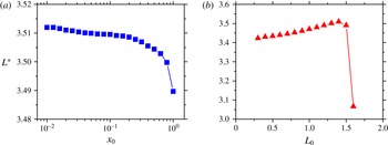
of the static meniscus. Figure 13(a) shows that the break-up height does not vary by more than 0.2 % within the range
 $0.01\leqslant x_{0}\leqslant 0.5$
. We have chosen to use the intermediate value
 $x_{0}=0.1$
in order to avoid the large thickness gradients in the vicinity of the liquid bath (arising when
 $x_{0}$
is too close to zero), while keeping a reasonably large initial domain (of length
 $L_{0}-x_{0}$
).
Predictions of the model for the influence of (a) the position
 $x_{0}$
in the static meniscus at which the boundary conditions are imposed (
 $L_{0}=\sqrt{2}$
being fixed) and (b) initial height of the static meniscus
 $L_{0}$
(
 $x_{0}=0.1$
being fixed). The pulling velocity and fibre half-width are
 $U=1~\text{mm}~\text{s}^{-1}$
(
 $Ca=0.047$
) and
 $H=50~\unicode[STIX]{x03BC}\text{m}$
(
 $\unicode[STIX]{x1D700}=0.034$
) respectively.

Similarly figure 13(b) indicates that the initial position
 $L_{0}$
of the fibre does not change the value of
 $L^{\ast }$
by more than 2 % as long as
 $L_{0}$
is large enough compared with
 $x_{0}$
and less than or about
 $\sqrt{2}$
. In the simulations, the initial position of the fibre has thus been set to the maximal value within this range, namely
 $L_{0}=\sqrt{2}$
, in order to have the largest possible initial domain and therefore the most mesh elements, allowing to keep a good spatial resolution when the mesh is stretched during film pulling. Note that for
 $L_{0}>\sqrt{2}$
, the thickness profile of the initial static meniscus features a minimum (Heller Reference Heller2008), which may explain the drop in the film break-up height observed for initial film heights greater than
 $\sqrt{2}$
.
Appendix B. Streamlines in the vicinity of the rupture point
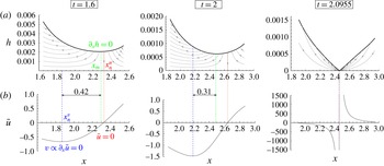
In this appendix, we compute the streamlines in order to visualise the flow in the vicinity of the rupture point. Figure 14(a) shows the streamlines for three different times,
 $t=1.6$
,
 $t=2$
and
 $t=2.0955$
, namely at rupture, during the pulling of a film with the same parameters as in figure 4. They were obtained by plotting the isocontours of the (dimensionless) streamfunction
 $$\begin{eqnarray}\unicode[STIX]{x1D713}=\int u\,\text{d}y=\bar{u}y+\unicode[STIX]{x1D700}^{2}\int u_{1}\,\text{d}y.\end{eqnarray}$$
The contribution of
 $u_{1}$
to the streamfunction
 $\unicode[STIX]{x1D713}$
was found to affect only marginally the streamlines; we thus used the approximation
 $\unicode[STIX]{x1D713}\approx \bar{u}y$
in figure 14(a). The corresponding average velocity profiles
 $\bar{u}(x)$
are displayed in figure 14(b).
Morphology of the flow in a film generated with a pulling velocity
 $U=1~\text{mm}~\text{s}^{-1}$
(
 $Ca=0.047$
), a fibre half-width
 $H=50~\unicode[STIX]{x03BC}\text{m}$
(
 $\unicode[STIX]{x1D700}=0.034$
) and a Hamaker constant
 $A_{H}=4.4\times 10^{-20}~\text{J}$
(same parameters as in figure 4). For three different times, we display (a) the streamlines (thin black lines) superimposed on the film thickness profiles (thick black lines) and (b) the average velocity profiles
 $\bar{u}(x)$
.

Several remarkable positions can be introduced:
-
(i) the point of minimum film thickness (green dash-dotted line in figure 14), located at a vertical position
$x_{m}$
and defined by
$\unicode[STIX]{x2202}_{x}h=0$
; -
(ii) the point where the vertical velocity
$\bar{u}$
changes sign (red dotted line in figure 14), located at
$x_{n}^{u}$
and defined by
$\bar{u}=0$
; -
(iii) the point where the horizontal velocity
$v$
changes sign (blue dashed in figure 14), located at
$x_{n}^{v}$
and defined by
$\unicode[STIX]{x2202}_{x}\bar{u}=0$
according to equation (2.18).


One can see from figure 14 that the minimum of film thickness
 $x_{m}$
is initially located close to the point of zero vertical velocity
 $x_{n}^{u}$
. As time goes by and the film is stretched,
 $x_{m}$
seems to be moving away from
 $x_{n}^{u}$
and getting closer to the point of zero horizontal velocity
 $x_{n}^{v}$
. All three points merge at the approach of film rupture (
 $t=2.0955$
).
Appendix C. Location of the puncture in the film
In addition to predicting the break-up height of the film, the model developed in § 2 also gives a prediction for the location of the puncture in the film (see e.g. figure 4
b), which calls for experimental verification. In this appendix, we sum up our observations regarding the bursting of silicone oil films, recorded with a high-speed camera (Photron Fastcam SA3) at frame rates ranging from
 $10\,000$
to
 $25\,000$
frames per second. We tested films made of
 $V350$
(pulling velocities
 $2{-}10~\text{mm}~\text{s}^{-1}$
),
 $V1000$
(pulling velocities
 $1{-}5~\text{mm}~\text{s}^{-1}$
) and
 $V10000$
(pulling velocities
 $0.3{-}1~\text{mm}~\text{s}^{-1}$
) silicone oils.
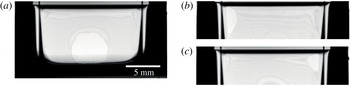
Our first observation was that the film thickness is not homogeneous in the horizontal direction (
 $z$
-axis), as can be seen qualitatively from the interference fringes in figure 15. This may be due to edge effects caused by the finite width of the film.
Some rupture events occur in the centre of the film (with respect to the
 $z$
-direction), as exemplified in figure 15(a). This is expected from our model, which assumes the film to be invariant along the
 $z$
-axis. Under the same conditions, some rupture events are also observed in the upper corners of the film, as shown in figure 15(b,c). However, the location of the puncture does not seem to affect the overall film lifetime, which was shown to be reproducible for a given capillary number (see figure 10). Thus, no matter where the film punctures, it bursts approximately at the same time, meaning that the thickness of the thin zones in the centre and upper corners of the film follows approximately the same time evolution.
High-speed observations of the bursting of films generated from a
 $V350$
silicone oil at a pulling velocity
 $U=10~\text{mm}~\text{s}^{-1}$
. The location of the puncture was not reproducible from one film to another and the films were observed to rupture (a) at the bottom centre, (b) in the upper left corner or (c) in the upper right corner.