


1. Introduction
Predictions of worldwide changes in glaciers in response to a changing climate rely on the use of models of glacier mass balance, i.e. glacier accumulation and ablation, as well as models describing the dynamics of ice flow. Ablation models of different complexity have been used to estimate glacier melt and mass balance, and for future predictions in particular (e.g. Reference Huss, Farinotti, Bauder and FunkHuss and others, 2008; Reference Hock, De Woul and RadicHock and others, 2009; Reference Farinotti, Usselmann, Huss, Bauder and FunkFarinotti and others, 2012; Reference Immerzeel, Van Beek, Konz, Shrestha and BierkensImmerzeel and others, 2012). For example, Reference Nolin, Phillippe, Jefferson and LewisNolin and others (2010) and Reference Hock, De Woul and RadicHock and others (2009) used a degree-day model, Reference Huss, Farinotti, Bauder and FunkHuss and others (2008) and Reference Farinotti, Usselmann, Huss, Bauder and FunkFarinotti and others (2012) employed a temperature-index model, including a shortwave radiation index, to simulate the response of Swiss glaciers to a changing climate and Reference Le Meur, Gerbaux, Schafer and VincentLe Meur and others (2007) used an energy-balance model for future simulations of the mass balance of an Alpine glacier.
For regional estimates of glacier changes (e.g. Reference Hock, De Woul and RadicHock and others, 2009), as well as for applications in data-scarce regions (Reference Ragettli and PellicciottiRagettli and Pellicciotti, 2012), melt models often need to be applied with little or no recalibration of model parameters. Even in the European Alps, applications outside the few well-studied glaciers rely on limited datasets that do not allow optimal calibration of all the parameters of a given model. The data most commonly available for model calibration and validation are glacier runoff (e.g. Reference Huss, Farinotti, Bauder and FunkHuss and others, 2008) and mass-balance data (e.g. Reference Finger, Pelliccotti, Konz, Rimkus and BurlandoFinger and others, 2011). The former, especially, does not allow internal validation of the model by testing that the single processes are correctly reproduced (Reference Pellicciotti, Buergi, Immerzeel, Konz and ShresthaPellicciotti and others, 2012), and might result in more than one set of parameter values providing the same model performance; this has been referred to as an ‘equifinality problem’ (Reference Beven and FreerBeven and Freer, 2001; Reference Wagener, McIntyre, Lees, Wheater and GuptaWagener and others, 2003; Reference BevenBeven, 2006).
In view of this limitation, there is a strong need to identify which parameters melt models are sensitive to, and which could be discarded from the calibration procedure because their impact on model output is small (Reference Saltelli, Tarantola and CampolongoSaltelli and others, 2000). This is particularly important for empirical models that rely more or less heavily on empirical parameters, such as the simple degree-day model and, to a lesser extent, enhanced versions of this approach (Reference HockHock, 1999; Reference Pellicciotti, Brock, Strasser, Burlando, Funk and CorripioPellicciotti and others, 2005). However, it is also relevant for more physically based approaches, such as energy-balance models, since when models are applied at the distributed scale, numerous additional parameters are introduced to extrapolate meteorological and surface variables (Reference MacDougall and FlowersMacDougall and Flowers, 2011).
Sensitivity analysis is a well-established technique in hydrological modelling (e.g. Reference McCuenMcCuen, 1973; Reference Saltelli, Tarantola and CampolongoSaltelli and others, 2000; Reference Kunstmann, Krause and MayrKunstmann and others, 2006; Reference Tang, Reed, Wagener and Van WerkhovenTang and others, 2007) which serves several purposes. One of these is to identify the most influential parameters on a given metric of model performance or output (Reference McCuenMcCuen, 1973; Reference Saltelli, Tarantola and CampolongoSaltelli and others, 2000). Less common is its use in studies of glacier mass balance and runoff, but some examples do exist (e.g. Reference Klok and OerlemansKlok and Oerlemans, 2002; Reference Hock and HolmgrenHock and Holmgren, 2005; Reference Pellicciotti, Brock, Strasser, Burlando, Funk and CorripioPellicciotti and others, 2005; Reference Anslow, Hostetler, Bidlake and ClarkAnslow and others, 2008; Reference MacDougall and FlowersMacDougall and Flowers, 2011; Reference MacDougall, Wheler and FlowersMacDougall and others, 2011; Reference Fitzgerald, Bamber, Ridley and RougierFitzgerald and others, 2012), all of which include analysis of model sensitivity to parameters in the melt modelling. However, most of these studies consider the model sensitivity to only one or a few parameters, often those taken from the literature or where the estimates were known to be less accurate. To date, only Reference MacDougall and FlowersMacDougall and Flowers (2011), Reference MacDougall, Wheler and FlowersMacDougall and others (2011) and Reference Fitzgerald, Bamber, Ridley and RougierFitzgerald and others (2012) have analysed the sensitivity of a distributed melt or mass-balance model to single variations in all of its parameters.
Several sensitivity methods exist. A main difference is between local and global approaches. In local methods, normally associated with so-called ‘one factor at a time’ (OAT) changes in parameters, the local response of the outputs, obtained by varying the factors one at a time, is investigated, while holding all other factors fixed to a central (optimal) value (Reference Saltelli, Tarantola and ChanSaltelli and others, 1999). In global methods, the space of the parameters is explored within a finite, larger region and factors are changed at the same time, so that the variation in model output induced by a factor is taken globally. The main disadvantage of local, OAT methods is that they do not consider parameter interaction, making them prone to underestimate the true model sensitivities (Reference McCuenMcCuen, 1973; Reference Saltelli, Tarantola and CampolongoSaltelli and others, 2000). However, they have the advantage of being straightforward to implement, while maintaining modest computational demands. Alternatively, global sensitivity methods vary all model parameters in predefined regions to determine their importance and potentially quantify the importance of parameter interactions.
Model sensitivity is closely related to model uncertainty (Reference Iman and HeltonIman and Helton, 1988). While sensitivity analysis involves determination of the changes in the response of a model to changes in individual model parameters, uncertainty analysis involves the determination of the variation or imprecision in model output that results from the (collective) variation in the model parameters (or input variables). Therefore, sensitivity can also be regarded as a tool to identify the important contributors to the uncertainty in model output (Reference Iman and HeltonIman and Helton, 1988).
In this work, we explore the parameter sensitivity and uncertainty of a distributed, enhanced temperature-index (ETI) melt model that was developed by Reference Pellicciotti, Brock, Strasser, Burlando, Funk and CorripioPellicciotti and others (2005) for Haut Glacier d’Arolla, Switzerland, and applied to several other locations and glacierized basins (Reference PellicciottiPellicciotti and others, 2008; Reference Finger, Pelliccotti, Konz, Rimkus and BurlandoFinger and others, 2011; Reference Petersen and PellicciottiPetersen and Pellicciotti, 2011; Reference Ragettli and PellicciottiRagettli and Pellicciotti, 2012). The model is of intermediate complexity between simple temperature-index and physically based energy-balance approaches. High temporal and spatial resolution in simulated melt rate is achieved by including variations in incoming shortwave radiation and albedo, and separating temperature-dependent and temperature-independent energy sources (Reference Pellicciotti, Brock, Strasser, Burlando, Funk and CorripioPellicciotti and others, 2005). The drawback of this approach is that the parameters might need recalibration for different melt seasons and glaciers. Reference Ragettli and PellicciottiRagettli and Pellicciotti (2012) showed that the model parameters needed recalibration for a glacier in the dry Andes, but the parameters of the melt equation, once recalibrated, were stable from one melt season to another. This study was based on a large amount of glacio-meteoro-logical data collected in the field over two ablation seasons. However, such data are not always available. For recalibration, therefore, it is of relevance to know the parameters that are crucial for the model outcome and hence should be known with a high degree of confidence for a sound model performance. Accordingly, our work has two main aims:
-
1. To identify which parameters most affect the ETI model outputs, i.e. which parameters the model is most sensitive to, and
-
2. To quantify the uncertainty associated with small variations in the parameters.
Several authors have indicated that sensitivity depends on the period and case study considered (e.g. Reference McCuenMcCuen, 1973). Reference MacDougall and FlowersMacDougall and Flowers (2011) showed that the sensitivity of a distributed energy-balance model was different for two neighbouring glaciers. For this reason, we apply the sensitivity analysis to different modelling periods and glaciers, in order to test the robustness of our results and avoid conclusions that are time- or site-specific.
We investigate the parameter sensitivity in a systematic manner in terms of the number of parameters changed, the different conditions (day, night, clear-sky, overcast) during one season on one glacier, different melt seasons and glaciers. We use meteorological and ablation datasets from two Alpine glaciers, Haut Glacier d’Arolla (ablation seasons 2001, 2006) and Gornergletscher (ablation season 2006), and from Glaciar Juncal Norte (ablation season 2008/09) located in the semi-arid Andes of central Chile. As a first step we analyse parameter sensitivity according to an OAT method for different seasons and glaciers to reveal the most sensitive parameters (aim 1 above). For Haut Glacier d’Arolla in 2001 we also check the ranking of parameter sensitivity changes under different conditions (day, night, clear-sky, overcast) in one melt season. In a second step, we investigate the optimality of the parameters at the distributed scale and the model uncertainty corresponding to a fixed amount of uncertainty in model parameters (aim 2) for Haut Glacier d’Arolla during the 2001 ablation season.
2. Study Sites and Data
2.1. Study sites
Haut Glacier d’Arolla is situated at the head of the Val d’Herens, Valais, Switzerland. The glacier is ∼ 4 km long, has an area of ∼6.3 km2 and ranges in elevation from 2560 to 3540ma.s.l. (Fig. 1). It consists of an upper basin with northwesterly aspect feeding a northward-flowing glacier tongue (Reference Pellicciotti, Brock, Strasser, Burlando, Funk and CorripioPellicciotti and others, 2005).
Map of Haut Glacier d’Arolla showing the glacier area (in grey), the watershed border and the position of the AWSs and ablation stakes in the 2001 ablation season.

Gornergletscher is located in Valais, at the head of the Mattertal. It is a polythermal glacier with areas of cold ice at temperatures below the pressure-melting point. It has a length of 14 km, covers a total area of 57.5 km2 and ranges in elevation from 2000 to 4600 ma.s.l. The glacier tongue covers an elevation range from 2600 to 2300 m a.s.l. Both sides of the tongue are covered with debris (Reference MullerMuller, 2010).
Glaciar Juncal Norte is located in the upper Aconcagua river basin, in the semi-arid Andes of central Chile. The glacier is ∼7.5 km long, has an area of ∼7.6 km2 and ranges in elevation from 2900 to 6100 m a.s.l. (Reference PellicciottiPellicciotti and others, 2008). The semi-arid Andes of central Chile are characterized by a pronounced seasonality, with runoff in summer (December-February) originating mainly from snow and glacier melt (Reference Pe*******na and NazaralaPe∼na and Nazarala, 1987; Reference Masiokas, Villalba, Luckman, Le Quesne and AravenaMasiokas and others, 2006), and precipitation largely absent (Reference PellicciottiPellicciotti and others, 2008). Most of the annual precipitation occurs in winter (June-August).
2.2. Meteorological and ablation measurements
The meteorological and ablation datasets collected on Haut Glacier d’Arolla during the 2001 and 2006 ablation seasons (referred to as HGdA01 and HGdA06, respectively) are described in more detail by Reference Strasser, Corripio, Pellicciotti, Burlando, Brock and FunkStrasser and others (2004), Reference Pellicciotti, Brock, Strasser, Burlando, Funk and CorripioPellicciotti and others (2005) and Reference Carenzo, Pellicciotti, Rimkus and BurlandoCarenzo and others (2009). Here we use data from two automatic weather stations (AWSs) on- and off-glacier (Fig. 1). AWS 1 was installed on the glacier in the two ablation seasons and recorded the following meteorological variables: air temperature (8C) and relative humidity (%) (with shielded and artificially ventilated sensors), wind speed (ms∼1) and direction (8) and incoming and reflected shortwave radiation (WmT2 ) . Sensors were fixed at 2 m above the surface on a tripod which could lower along with the melting surface to maintain a constant distance between the sensors and the surface. Measurements were taken every 5 s and the average stored every 5 min on Campbell CR10 and CR10X data loggers. The data were aggregated to hourly averages. The proglacial station AWS 0 (Fig. 1) recorded the same variables and also precipitation and incoming and outgoing longwave radiation (Reference Pellicciotti, Brock, Strasser, Burlando, Funk and CorripioPellicciotti and others, 2005).
Ablation was measured at stakes installed on the glacier (see Fig. 1). The first stake readings were performed on 21 July and the last on 15 August. The number of readings differs from stake to stake (from 2 readings up to 12, with, on average, 7.5 readings at each stake).
In the 2006 ablation season on Gornergletscher (referred to as GG06) one station on the glacier (AWS 1) and a station installed on the lateral slopes (AWS 0) were operated. The glacier station, AWS 1 , recorded the same variables as on Haut Glacier d’Arolla, while the proglacial station recorded temperature and precipitation. (See Reference Carenzo, Pellicciotti, Rimkus and BurlandoCarenzo and others, 2009, and Reference MullerMuller, 2010, for details of sensors, set-up and recorded variables.)
For the 2008/09 ablation season on Glaciar Juncal Norte (referred to as JNG08/09), two stations, AWS 1 and AWS 3, were installed on the tongue of the glacier and in the proglacial valley, respectively. The stations recorded the same meteorological variables as those on Haut Glacier d’Arolla (Reference Ragettli and PellicciottiRagettli and Pellicciotti, 2012). (Details of the setup and measurements are provided by Reference PellicciottiPellicciotti and others, 2008, and Reference Ragettli and PellicciottiRagettli and Pellicciotti, 2012.)
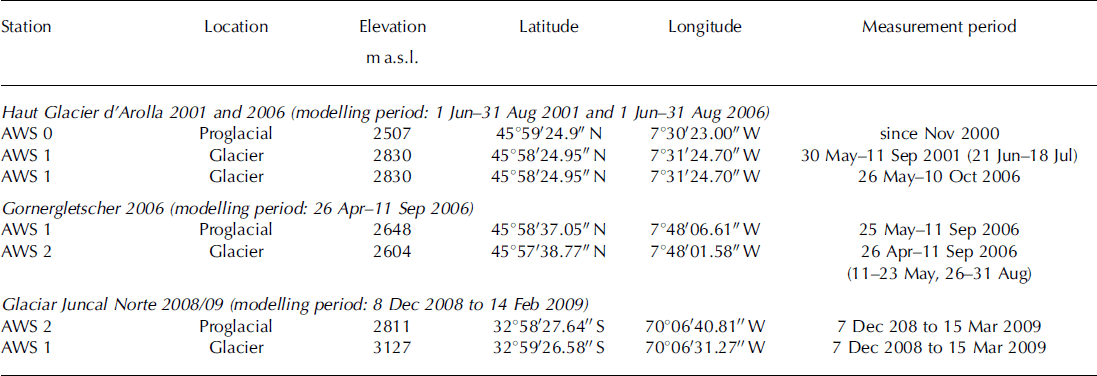
The measurement periods and coordinates of all AWSs are given in Table 1 . For each case study, data from the on-glacier AWS are used to force the model. The off-glacier AWS provides data for calculation of the cloud factor and precipitation measurements.
Measurement periods, modelling periods and coordinates of the AWSs for all glaciers and melt seasons. In parentheses after the measurement period are periods of data gaps
2.3. Initial snow depth
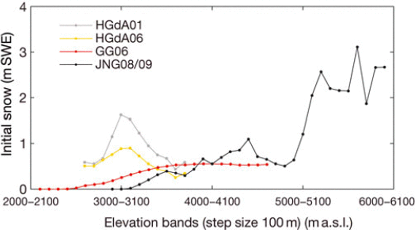
Initial conditions of snow depth are required to run the model simulations. Initial snow depth was estimated for every gridcell of the watershed on all three glaciers, by linear extrapolation of snow depth measurements taken on each glacier at the beginning of the observation period. On Gornergletscher and Glaciar Juncal Norte, measurements were mostly carried out on the lower sections of the glacier, because of restricted access (see Reference MullerMuller, 2010; Reference Ragettli and PellicciottiRagettli and Pellicciotti, 2012, for the locations). The initial snow depth observations were interpolated using an elevation gradient and corrected with a residual field (based on the inverse distance method) to obtain a map of gridded values of initial snow water equivalent (Reference MullerMuller, 2010). If the slope of a watershed cell was >458, initial snow depth was set to zero. Snow depths were converted to snow water equivalent (SWE) by means of measured density. Density was measured on each glacier at the time of the snow depth survey at one or two locations. (Details of the measurements are given by Reference Pellicciotti, Brock, Strasser, Burlando, Funk and CorripioPellicciotti and others, 2005; Reference Carenzo, Pellicciotti, Rimkus and BurlandoCarenzo and others, 2009; Reference MullerMuller, 2010; Reference Ragettli and PellicciottiRagettli and Pellicciotti, 2012.) Because of the simple extrapolation used and the discrete nature of the observations of snow depth and density, the initial distribution of SWE is subject to uncertainty. This might influence the model performance and its ability to reproduce the evolution of the snowpack. Figure 2 shows the initial SWE distribution per elevation band (bandwidth 100 m) for every glacier and melt season. On Haut Glacier d’Arolla there was considerably more snow at the beginning of the season in 2001 than in 2006. For both GG06 and JNG08/09 there was less snow at the beginning of the simulation and it was mainly located at higher altitudes, where temperatures are low and the snow is unlikely to melt (Reference Ragettli and PellicciottiRagettli and Pellicciotti, 2012).
Initial snow water equivalent of the watershed per 100 m elevation band, normalized by the number of model gridcells per elevation band for every glacier and melt season.
3. Ablation Model
In the distributed ETI model, melt rate, M (mmw.e. h∼1), is computed as (Reference Pellicciotti, Brock, Strasser, Burlando, Funk and CorripioPellicciotti and others, 2005, Reference Pellicciotti2008; Reference Ragettli and PellicciottiRagettli and Pellicciotti, 2012):

where T is the hourly mean air temperature at the screen level (°C), a is the albedo and I is the incoming shortwave radiation (Wm∼2 ) . The temperature factor, TF (mmh∼1 oC∼1 ) , and shortwave-radiation factor, SRF (m2 mm W∼1 h∼1), are empirical parameters. TT is a threshold temperature above which melt is assumed to occur.
Incoming shortwave radiation in every gridcell is computed using a non-parametric clear-sky model based on that of Reference IqbalIqbal (1983) and described in detail by Reference Pellicciotti, Raschle, Huerlimann, Carenzo and BurlandoPellicciotti and others (2011). Terrain parameters and the solar position, as well as the interaction between solar radiation and the topography, are derived using the vectorial algebra approach of Reference CorripioCorripio (2003). The only parameters needed in the clear-sky solar radiation model are the visibility, vis, and ozone layer thickness, O3. The net effect of clouds is modelled using cloud transmittance factors, ctf, computed as a function of the diurnal temperature range, following Reference Pellicciotti, Raschle, Huerlimann, Carenzo and BurlandoPellicciotti and others (2011). Use of a daily cloud factor to account for the effect of clouds on the clear-sky global irradiance is a widely used approach in mesoscale atmospheric studies (e.g. Reference Thornton and RunningThornton and Running, 1999; Reference Pfister, McKenzie, Liley, Thomas, Forgan and LongPfister and others, 2003; Reference Fitzpatrick, Brandt and WarrenFitzpatrick and others, 2004) and it has recently been used in distributed models of glacier melt (Reference Klok and OerlemansKlok and Oerlemans, 2002; Reference Anslow, Hostetler, Bidlake and ClarkAnslow and others, 2008; Reference Ragettli and PellicciottiRagettli and Pellicciotti, 2012). The approach is based on the relationship between daily cloud transmittance, ctf, and the daily temperature range:

where ΔT is the daily temperature range measured at an off-glacier station and cf1 and cf2 are empirical coefficients (Reference Pellicciotti, Raschle, Huerlimann, Carenzo and BurlandoPellicciotti and others, 2011). To avoid underestimating the clear-sky days radiation, a cloud factor threshold, cft is used, following Reference Pellicciotti, Raschle, Huerlimann, Carenzo and BurlandoPellicciotti and others (2011). Cloud factor values greater than or equal to this threshold are set to 1, which corresponds to clear-sky conditions.
The albedo of ice, aice, and of the surrounding bare terrain, abg, (the latter used in the solar radiation model; Reference Pellicciotti, Raschle, Huerlimann, Carenzo and BurlandoPellicciotti and others, 2011) are assumed to be constant. Daily snow albedo is calculated using two different parameterizations: (1) the US Army Corps of Engineers (1956) approach and (2) the parameterization of Reference Brock, Willis and SharpBrock and others (2000). In the first parameterization, snow albedo, as, is assumed to decay exponentially with the number of days, n, since the last significant snowfall, ss:

where a1us, «2us and kpos,neg are empirical parameters. k differs for positive and negative temperatures.
According to Reference Brock, Willis and SharpBrock and others (2000), daily snow albedo is computed as a logarithmic function of the accumulated daily maximum positive air temperature, Tacc (°C), since the last significant snowfall, ss:

where a1br and a2br are empirical parameters.
Temperature and precipitation measured at the point scale of the AWSs are extrapolated to the gridcells of the watershed with a temperature lapse rate, LR (°Cmr1) , that is constant in time, and uniform in space and precipitation gradient, Tp (mm mr1 ) . To distinguish between solid and liquid precipitation a simple phase threshold, pht (°C), is used.
In addition to the melt parameters for temperate, debris-free ice (SRF and TF), separate values for cold ice and debris-covered ice for the ETI model were introduced by Reference MullerMuller (2010) for GG06, to take into account the different surface characteristics of Gornergletscher. These are: SRFcoldice, SRFdebrisice, TFcoldice, TFdebrisice and are also considered in the sensitivity analysis.
4. Sensitivity to Individual Parameters
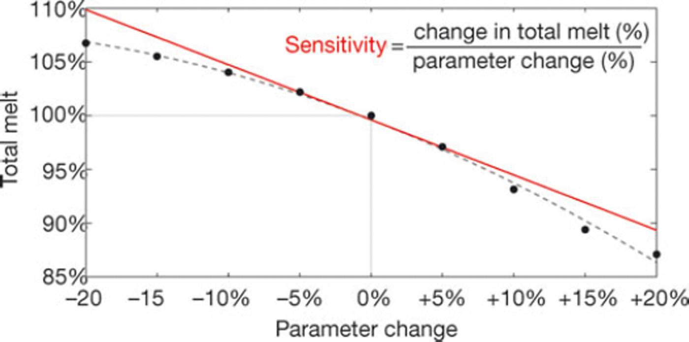
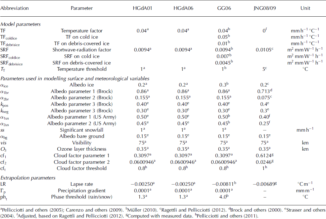
The approach used to compute the sensitivity to individual parameters is an OAT method, adopted from Reference Anslow, Hostetler, Bidlake and ClarkAnslow and others (2008) and Reference Ragettli and PellicciottiRagettli and Pellicciotti (2012). The method was also used by Reference MacDougall and FlowersMacDougall and Flowers (2011). This is a well-established method for calculation of model sensitivity (e.g. Reference McCuenMcCuen, 1973; Reference Saltelli, Tarantola and ChanSaltelli and others, 1999). We varied the parameters about the optimal value in 5% increments from —20% to +20%. We use a larger range than commonly adopted to investigate the linearity of the model response. In each model run, one parameter was changed while the others remained fixed at their optimal value. For every parameter change, the modelled total melt (cumulative seasonal melt occurring over the whole watershed) was computed as a percentage of the total melt modelled with the optimal value. Sensitivity was calculated by fitting a second-order polynomial to these results for a given parameter and then determining the slope of the polynomial about the optimal value (Fig. 3). (Details of the methods are given by Reference Ragettli and PellicciottiRagettli and Pellicciotti, 2012.) The optimal parameter values were calibrated in ad hoc studies at the point scale, except for the extrapolation parameters. Their sources are listed in Table 2.
Illustration of the method used to determine the sensitivity of individual parameters: change in total melt is plotted against the corresponding change in a given parameter. The dashed grey line is the fitted second-order polynomial and the red line indicates the slope around the optimal value used as measure for the sensitivity.
Optimal parameters for the sensitivity analysis to individual parameter changes
The analysis was performed separately for total melt over the entire basin, on the glacier and on the non-glacierized slopes. We also considered, separately, sensitivity for the daily minimum melt, daily mean melt, daily maximum melt and daily standard deviation of melt, spatially averaged over the whole watershed and temporally averaged over the number of modelling days. These statistics are referred to here as ‘daily min’, ‘daily mean’, ‘daily max’ and ‘daily stdv’, respectively. A positive sensitivity denotes that an increase in the parameter causes an increase in total melt; a negative sensitivity that an increase in the parameter results in a reduction in melt. All model runs were conducted using the US Army Corps of Engineers (1956) approach for albedo, except for the separate, specific runs to assess the model sensitivity to the parameters a1br and a2br of the Reference Brock, Willis and SharpBrock and others (2000) parameterization.
The method used implies that the initial parameter values are the optimal ones, otherwise sensitivity is meaningless, as it could be conducted in any region of the parameter space with little relevance in terms of model performance. Parameter optimization depends, however, on the period considered, optimization methods and type of input data used to force the models (measured or simulated) and validation datasets employed to define the model performance, as well as the spatial scale of the model application. Parameters optimized at the point scale, as by Reference Pellicciotti, Brock, Strasser, Burlando, Funk and CorripioPellicciotti and others (2005) or Reference Carenzo, Pellicciotti, Rimkus and BurlandoCarenzo and others (2009), might not be the optimal ones for distributed applications of the model. The assumption that the optimal parameters (calibrated at the point scale) used in this work are also the optimal values at the distributed scale is considered in Section 5.
In general, the parameter values for Haut Glacier d’Arolla are likely to be optimal also at the distributed scale of this application, because Haut Glacier d’Arolla is a small glacier where variability in surface and meteorological conditions can be expected to be small. The glacier has also been extensively investigated (e.g. Reference Brock, Willis and SharpBrock and others, 2000; Reference Pellicciotti, Brock, Strasser, Burlando, Funk and CorripioPellicciotti and others, 2005, Reference Pellicciotti, Raschle, Huerlimann, Carenzo and Burlando2011; Reference Carenzo, Pellicciotti, Rimkus and BurlandoCarenzo and others, 2009), so quite a large dataset of observations exists for model calibration. For the two other glaciers, more uncertainty is to be expected, given the more limited datasets used to optimize the model parameters and the glaciers’ larger elevation ranges and types of surface characteristics.
For JNG08/09 the optimal value of TF is zero (Reference Ragettli and PellicciottiRagettli and Pellicciotti, 2012), therefore this parameter is varied from 0 to 0.016, which corresponds to the range over which it is varied for HGdA01, HGdA06 and GG06. The same applies to the optimal cloud factor threshold which is equal to 1 and hence is changed from 0.67 to 1.00.
To estimate whether parameter sensitivity is robust to different conditions, we performed the analysis separately for the following four conditions for Haut Glacier d’Arolla ablation season 2001: (1) day, (2) night, (3) clear-sky and (4) overcast. The sensitivity during daytime and night-time was determined by considering the melt in the hours 08:00–22:00 and 22:00–08:00, respectively. To distinguish between clear-sky and overcast days an algorithm developed by Reference Carenzo, Pellicciotti, Rimkus and BurlandoCarenzo and others (2009) was used. Since the conditions analysed are largely independent of the climatic setting, we do not expect large differences among sites, and we carried out the analysis only for HGdA01.
5. Parameter Optimality at the Distributed Scale and Model uncertainty for HGdA01
To test that parameters are optimal at the distributed scale and quantify model uncertainty we use a Monte Carlo approach. The same method was employed by Reference Anslow, Hostetler, Bidlake and ClarkAnslow and others (2008) and Reference Ragettli and PellicciottiRagettli and Pellicciotti (2012). A total of 104 model realizations were obtained by randomly selecting model parameters from a uniform distribution out of a range vector with parameter changes from –5% to +5% around the optimal value (with a step size of 1%). By plotting the model performance associated with each model run we can evaluate whether the optimal parameter values at the point scale are also optimal at the distributed scale in the space searched by the Monte Carlo simulations. For every run, we plotted the total melt against the corresponding root-mean-square error, rmse, at the ablation stakes (Fig. 1).
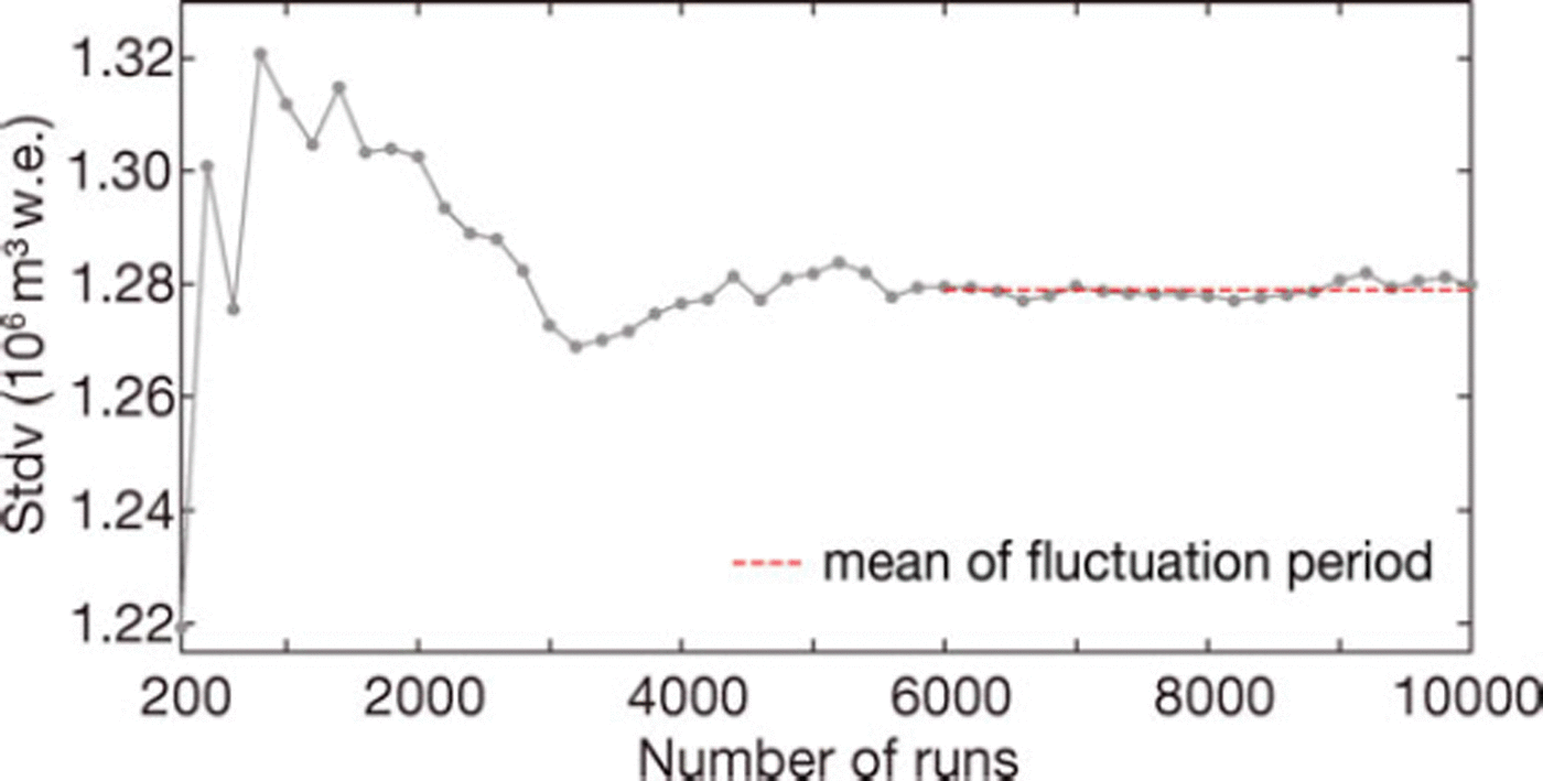
The standard deviation, stdv, of the total melt for the 104 runs provides a measure of the uncertainty in model outcome that is associated with a particular amount of uncertainty in model parameters (Reference Ragettli and PellicciottiRagettli and Pellicciotti, 2012). Because stdv depends on the number of runs, we plotted it against the number of runs and verified that stdv stabilizes around a particular value within the 104 runs. We then took the mean of the stdv during the period after which no further important changes in stdv are evident.
To determine model uncertainty it is crucial to perform the 104 runs with parameters which are near their optimal value at the distributed scale. We therefore performed 103 preliminary runs with the optimal values calibrated at the point scale, validated them against the stake readings, identified a new optimal value and started the 104 realizations with the new parameter set.
In the assessment of the sensitivity of individual parameters (Section 4), the albedo parameters from the parameterization of Reference Brock, Willis and SharpBrock and others (2000) were found to be more sensitive than those of the US Army Corps of Engineers (1956) model. Therefore for the model uncertainty simulations, albedo was computed based on the parameterization of Reference Brock, Willis and SharpBrock and others (2000).
6. Results
6. 1. Sensitivity to individual parameters
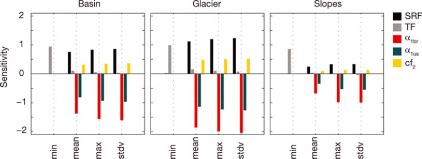
Figure 4 shows the magnitude of calculated sensitivity for the most sensitive parameters (sensitivity >0.5 for basin section: glacier) for the different basin sections and the four daily melt statistics for HGdA01. Parameter sensitivity ranking is consistent across different basin sections and daily statistics, except for the minimum melt. The same results were obtained for all melt seasons and glaciers examined and are not reported here, for reasons of space. For HGdA01 the parameters to which the model is most sensitive to are the parameters related to the modelling of the shortwave-radiation flux, i.e. SRF (Eqn (1)), a1br and a1us, as well as cf2. Minimum melt, by contrast, is controlled by the temperature factor, TF, of the melt equation (Eqn (1)). Since mean and maximum melt are more relevant than minimum melt for assessment of glacier melt, we concentrate on the model sensitivity with respect to these, and consider minimum melt no further here.
Sensitivity of parameters (reported only for those parameters with a sensitivity >0.5 on the glacier) for HGdA01. Sensitivity is depicted separately for the different basin sections (total basin, glacier area and non-glacierized slopes) and for different daily statistics: minimum total melt (min), mean total melt (mean), maximum total melt (max) and standard deviation of total melt (stdv). Sensitivity is given as % melt change per % parameter change (dimensionless).
In Table 3, the top ten parameters to which the model is most sensitive are listed for the different melt seasons and glaciers. In contrast to glacier ice, the amount of snow on the slopes is limited during one ablation season and this affects parameter sensitivity. On the slopes, an increase in melt rate is reflected in parameter sensitivity only if additional snow is available for melt. Similarly, small reductions in melt rates might still be sufficient to melt all the snow if there is only a limited amount, and therefore the model would be equally sensitive to the parameters. Therefore sensitivity on the non-glacierized slopes strongly depends on the amount of snow available, which in turn depends on the initial SWE and solid precipitation.
Top ten parameters to which the model is most sensitive and corresponding sensitivity, calculated for mean daily glacier melt, ranked from highest to lowest sensitivity, for all the glaciers and melt seasons considered
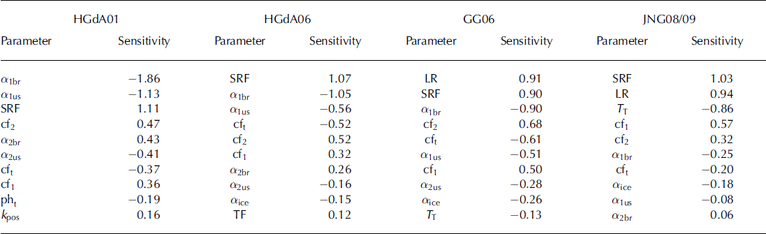
Uncertainty in the initial snow conditions or in the distribution of the ablation season precipitation might therefore affect the results. Hence we focus on the sensitivity in the basin as a whole and on the glacier where this influence is smaller. The parameter ranking for ‘daily mean’, ‘daily max’ and ‘daily stdv’ is, except for minor differences, the same for the basin, and the ranking for the basin is the same as for the glacier. Therefore only the ranking of ‘daily mean’ melt on the glacier is shown.
Results are consistent for the different sites (Table 3). Mean melt, together with its daily variation (stdv) and maximum melt, is controlled by the parameters influencing the shortwave-radiation-dependent term of the melt equation (Eqn (1)). There are some differences in the actual magnitude and ranking of the sensitivities, but the first eight parameters for all sites and seasons are the SRF, the albedo parameters and the coefficients of the cloud factor parameterization (Table 3). In addition to these, important parameters are the LR for both Gornergletscher and Glaciar Juncal Norte and TT for Glaciar Juncal Norte. For all the glaciers the empirical parameter, SRF, is among the most sensitive (Table 3). For Alpine glaciers, where summer precipitation is important, the model is sensitive to the albedo parameters, a1br and a1us, in contrast to JNG08/09, where precipitation is largely absent. The model is sensitive to cloud factor parameters across melt seasons and glaciers (Table 3).
On the non-glacierized slopes, where only snowmelt can occur, the albedo parameters, a1br and a1us, and the SRF are important, as well as LR, TT and pht . The latter control the amount of snow available for melt, either by increasing the number of cells where melt occurs (LR and TT) or by increasing the amount of solid precipitation (pht).
6.2. Sensitivity under different conditions
Figure 5 depicts the parameter sensitivity on HGdA01 for different conditions over one season (as well as for the entire period of record). Since the sensitivities for ‘daily mean’, ‘daily max’ and ‘daily stdv’ are very similar, only the sensitivity for ‘daily mean’ is shown.
Parameter sensitivity under specific conditions during the melt season compared to all conditions (black bars, indicated as ‘allcond’ in legend) for ‘daily mean’ melt on HGdA01.
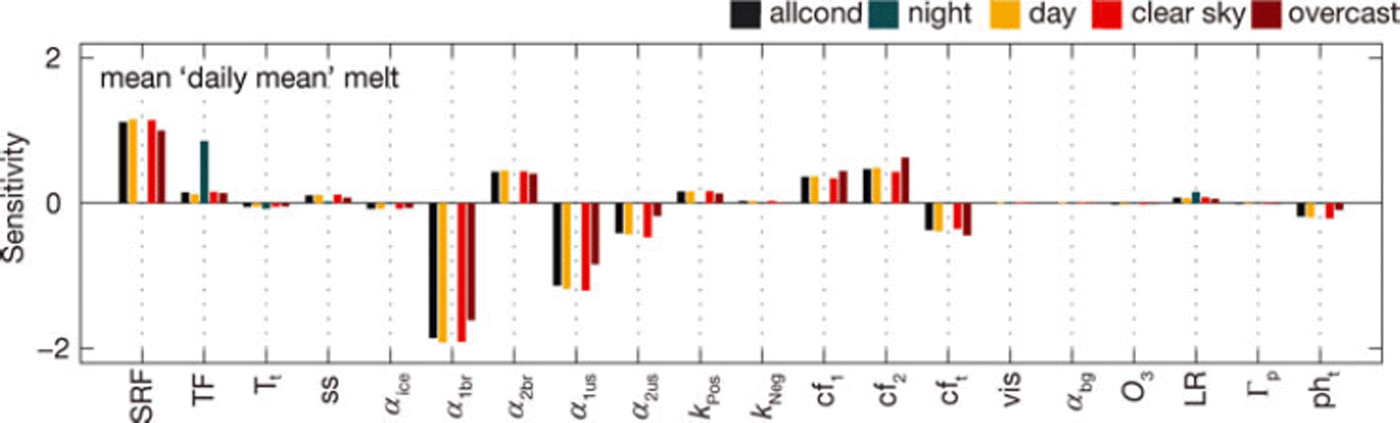
During daytime, the sensitivity of the incoming shortwave-radiation-related parameters is slightly increased compared to the entire period of record. During night-time (22:00-08:00), I is absent for most of the hours and therefore the model is not very sensitive to I-related parameters. Model sensitivities under clear-sky conditions are basically the same as for the entire period of record (Fig. 5). Under overcast conditions, however, sensitivities are markedly distinct. The parameters a1br, a1us and SRF become less important (with a decrease in model sensitivity of ∼15%), while the cloud factor parameters are more important (by ∼25%).
6.3. Parameter optimality at the distributed scale and model uncertainty for HGdA01
Figure 6 shows total melt plotted against the corresponding rmse for every run, for HGdA01. The rmse is calculated by comparing modelled and measured melt at the ablation stakes and is used here as an indication of the best model performance. In Figure 6a the 103 preliminary runs are depicted and Figure 6b shows the 104 runs where the parameter set with the lowest rmse of the 103 preliminary runs was used as the starting point.
Total melt and corresponding rmse of the model realizations conducted to estimate model uncertainty and investigate whether parameters fall in the optimal region at the distributed scale, for HGdA01. (a) 103 preliminary runs and (b) 104 final runs. The standard deviation depicted is the mean stdv in Figure 7.
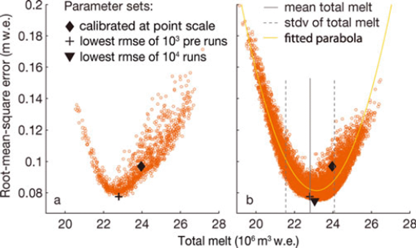
The optimal set calibrated at the point scale is within one standard deviation of the optimum identified with the 104 realizations (Fig. 6). Compared to the run with the lowest rmse (indicated by the triangle), total melt was overestimated by 4%. The parameter values calibrated at the point scale were compared to the parameter values of the new optimal run (i.e. the run with the lowest rmse in Fig. 6b). Considering all parameters, parameter values change on average by <3%, and considering only the most sensitive parameters (sensitivity >0.5 on the glacier) values change on average by only 2%. This is an indication that, albeit with some margin for improvement, the parameter set calibrated at the point scale is nearly optimal.
The development of the standard deviation (stdv) is shown in Figure 7, together with the mean standard deviation of the 104 model realizations, for HGdA01. After ∼6000 runs stdv starts to fluctuate around a mean value of 1:28 × 106 m3 w.e., which corresponds to 5.6% of the mean total melt of the 104 runs.
Standard deviation of the total melt against the number of runs (step size 200 runs) used to compute the standard deviation, for HGdA01. The dashed red curve is the mean standard deviation for the fluctuation period from run 6000 to run 104.
7. Discussion
7.1. Sensitivity to individual parameters
One of the main findings of our work is that the model is most sensitive to parameters controlling the net shortwave-radiation flux. The much higher sensitivity of the shortwave-radiation-related parameters compared to temperature-dependent parameters depends partly on the nature of the model, in which the shortwave-radiation flux is explicitly included. However, it also indicates that the shortwave-radiation flux is the dominant source of melt energy for glaciers in the climatic settings considered, as found by numerous modelling studies (e.g. Reference Greuell and SmeetsGreuell and Smeets, 2001; Reference Willis, Arnold and BrockWillis and others, 2002; Reference PellicciottiPellicciotti and others, 2008). This is particularly so for glaciers in the dry Andes of Chile, where incoming shortwave radiation is very high during the melt season and clouds are basically absent in summer (Reference PellicciottiPellicciotti and others, 2008; Reference Ragettli and PellicciottiRagettli and Pellicciotti, 2012). It might be different for glaciers such as maritime ones, where temperature-dependent energy fluxes (e.g. the sensible heat fluxes) are higher (Reference Giesen, Van den Broeke, Oerlemans and AndreassenGiesen and others, 2008). These results seem to be robust, as sensitivity ranking is consistent across the different basin sections, different conditions and the daily statistics examined.
For Alpine glaciers with precipitation events in summer, the snow albedo parameters have a key influence upon the spatial and temporal evolution of melt rates, in agreement with, for example, Reference Favier, Wagnon, Chazarin, Maisincho and CoudrainFavier and others (2004) and Reference Pellicciotti, Brock, Strasser, Burlando, Funk and CorripioPellicciotti and others (2005). The same results were obtained by Reference MacDougall and FlowersMacDougall and Flowers (2011) when analysing the sensitivity of an energy-balance model, even though the authors used a different albedo parameterization. Estimation of solid precipitation from point measurements is affected by uncertainties associated with both lack of knowledge about how best to extrapolate it in space and in its phase, as well as by undercatch errors at the gauges. For glaciers and seasons characterized by larger or more frequent summer precipitation it might be expected that the model is more sensitive to the parameters related to solid precipitation than revealed by the current analysis. However, this would not affect the ranking of the most sensitive parameters, as the model is already very sensitive to the albedo parameters (Table 3). Errors due to gauge undercatch might affect the sensitivity of the model to r p and pht . Undercatch errors are difficult to evaluate in the absence of accurate measurements of wind at the gauge (Reference Nespor and SevrukNespor and Sevruk, 1999; Reference Zweifel and SevrukZweifel and Sevruk, 2002) and these data were not available for Gornergletscher. Simpler constant correction factors would need calibration and would therefore compensate for any number of other errors, thus we did not use any in this study. Solid precipitation might therefore be underestimated and model sensitivity to the phase threshold and precipitation gradient might be higher. At our study sites, summer accumulation was relatively modest compared to total melt: summer accumulation is <5.4% of total ablation at the location of the AWSs at our three sites, and <7% for HGdA01 and HGdA06 when the wind-based correction for gauge undercatch of Reference Zweifel and SevrukZweifel and Sevruk (2002) is implemented (with total ablation calculated with an energy-balance model; Reference Carenzo, Pellicciotti, Rimkus and BurlandoCarenzo and others, 2009). The impact of the same correction on the summer mass balance at the distributed glacier scale is also minor, with differences in total ablation of 2 . 1% and 0.8% for HGdA01 and HGdA06, respectively, if we include the correction of Reference CarenzoCarenzo (2012).
For glaciers such as GG06 and JNG08/09 with a wide altitudinal range, LR is among the parameters to which the model is most sensitive, in agreement with findings of Reference Li and WilliamsLi and Williams (2008), Reference Gardner and SharpGardner and Sharp (2009), Reference Petersen and PellicciottiPetersen and Pellicciotti (2011) and Reference Ragettli and PellicciottiRagettli and Pellicciotti (2012). The high sensitivity of the model to the lapse rate and the increasing awareness that lapse rates that are uniform in space and constant in time are not appropriate for hydrological and glaciological studies (Reference Braun and HockBraun and Hock, 2004; Reference Li and WilliamsLi and Williams, 2008; Reference Gardner and SharpGardner and Sharp, 2009; Reference Minder, Mote and LundquistMinder and others, 2010; Reference Petersen and PellicciottiPetersen and Pellicciotti, 2011) point to the need for further investigation of the spatial and temporal variability of air temperature, and the way this is represented in melt and mass-balance models.
7.2. Optimal parameters and model uncertainty
Using Monte Carlo techniques it is possible to generate model realizations by randomly sampling the space of the parameters in a given interval, to verify that the parameters identified as optimal with any of numerous available methods (from manual calibration to automatic techniques, from local to global optimization methods) are indeed optimal in a global sense (Reference Iman and HeltonIman and Helton, 1988). A key issue in this type of analysis is the number of model realizations that guarantees that the entire relevant space of plausible parameters is sampled (Reference Finger, Pelliccotti, Konz, Rimkus and BurlandoFinger and others, 2011). Even though the 112 0 possible parameter set combinations (ten possible changes plus one initial value per parameter and 20 parameters) might seem too many compared to the 104 model runs performed for HGdA01, Figure 6 shows that 104 runs are enough to clearly develop the expected shape of a parabola and indicate that the shape is unlikely to change with additional runs. They also allow identification of the minimum in model error associated with the optimal parameter set. Although the identification of the optimal parameters depends on the dataset used (here stake measurements) and the optimization criterion (here rmse) employed to compare the model simulation with the observations (Reference Pellicciotti, Buergi, Immerzeel, Konz and ShresthaPellicciotti and others, 2012), our results indicate that the sensitive parameters calibrated at the point scale are also in the region of the optimal values at the distributed scale.
8. Conclusions
We have analysed the sensitivity of a distributed ETI melt model for a number of glaciers and seasons in the Swiss Alps and the central Andes of Chile, with the aim of identifying the parameters to which the model is most sensitive. By identifying the main parameters controlling the model behaviour, sensitivity analysis helps in deciding which parameters should be the focus of calibration (Reference Tang, Reed, Wagener and Van WerkhovenTang and others, 2007). This is important in general, but especially in cases where only limited datasets are available for calibration, such as in the Andes of Chile and in the Himalaya (Reference Pellicciotti, Buergi, Immerzeel, Konz and ShresthaPellicciotti and others, 2012). This type of investigation is particularly important to inform the design of field measurement campaigns (Reference Tang, Reed, Wagener and Van WerkhovenTang and others, 2007), especially for models of snow and ice melt that often require devoted field campaigns at sites that are remote and difficult to access. In this light, such analysis is useful to identify the data that need to be collected to constrain model parameters that are relevant to the modelling. Also, despite the fact that the ETI model has been applied in various investigations in different regions of the world (Reference Pellicciotti, Brock, Strasser, Burlando, Funk and CorripioPellicciotti and others, 2005, Reference Pellicciotti, Buergi, Immerzeel, Konz and Shrestha2012; Reference Carenzo, Pellicciotti, Rimkus and BurlandoCarenzo and others, 2009; Reference Finger, Pelliccotti, Konz, Rimkus and BurlandoFinger and others, 2011; Reference Ragettli and PellicciottiRagettli and Pellicciotti, 2012), this is the first study that analyses systematically, over several glaciers and seasons, its sensitivity to both model parameters and parameters controlling the extrapolation of the meteorological and surface variables used as input to the model.
Our main conclusions are as follows:
-
1. The parameters the model is most sensitive to are the shortwave-radiation factor, SRF, the air temperature lapse rate (especially for glaciers with a large elevation range), the albedo parameters (especially if precipitation is present), the cloud factor parameters and the temperature threshold (depending on the number of hours with temperatures close to TT).
-
2. These results are consistent across different basin sections, different meteorological conditions over one season and the daily statistics examined, as well as across melt seasons and glaciers, with some differences, that are explained by the different climatic and topographic characteristics of the glaciers.
-
3. These results are useful for calibration strategies, as they indicate which parameters should be the focus of calibration and thus of the design of devoted monitoring campaigns. In particular, our findings suggest, in agreement with several recent studies, that the LR used for extrapolation of air temperature to the glacier or basin scale should be known with accuracy, as the model is very sensitive to it, especially for large basins. More measurements of air temperature variability over glaciers are therefore encouraged (Reference Minder, Mote and LundquistMinder and others, 2010; Reference Petersen and PellicciottiPetersen and Pellicciotti, 2011).
-
4. Some of the parameters the model is most sensitive to are parameters of the equation used to calculate melt (e.g. SRF and TT). Others, however, are parameters related to the generation of distributed fields of input meteorological and surface variables (e.g. air temperature, albedo and shortwave radiation). Our results are therefore likely to be valid for any distributed model that requires such input data (including energy-balance models), as confirmed by the findings of Reference MacDougall and FlowersMacDougall and Flowers (2011), who also found a distributed energy balance was most sensitive to albedo parameters, and by those of Reference Fitzgerald, Bamber, Ridley and RougierFitzgerald and others (2012), who found the same results for an enhanced version of a temperature-index model.
-
5. The parameter values calibrated at the point scale for HGdA01 seem to be in the region of the optimal values at the distributed scale. Monte Carlo techniques, such as the one employed in this work, are a useful tool to test that the identified model parameters are optimal, also because in most cases only limited datasets are available for parameter calibration.
-
6. Finally, a parameter uncertainty of 5% results in a model uncertainty of 1:28 x 106 m3 w.e. for Haut Glacier d’Arolla, which corresponds to 5.6% of the mean total melt.
Acknowledgements
We thank Andreas Bauder and Albin Kretz, who participated in the data collection on Gornergletscher, and all the people who helped in the field campaign on Glaciar Juncal Norte, Jakob Helbing in particular. Paolo Burlando provided support for M.C. and the glacier field campaigns, and Ruzica Dadic provided the 2006 HGdA data. We also thank two anonymous reviewers for very useful comments.



