1. Introduction
The flow of a slurry is a problem that is relevant to many natural processes, such as mudflows or landslides, as well as to industrial applications, such as the flow of a cement slurry. This study, however, addresses the problem of slurry flow in the context of hydraulic fracturing that is relevant to oil and gas reservoir stimulation (Economides & Nolte Reference Economides and Nolte2000). Typically, proppant is used to prevent the fracture from closing once the well is depressurized. In this case, modelling the fracture propagation driven just by a viscous fluid is not sufficient, since the proppant, blended with the fracturing fluid, alters the properties of the latter. In this situation, it is necessary to consider the effects associated with the flow of a slurry as well as the proppant transport in hydraulic fractures. As mentioned in Adachi et al. (Reference Adachi, Siebrits, Peirce and Desroches2007), for the purpose of hydraulic fracturing, the slurry is typically modelled as a Newtonian fluid, whose viscosity dependence on proppant content is calculated based on an empirical formula. Moreover, the particle distribution across the fracture is assumed to be uniform and only the slip velocity due to gravity is considered. While all the aforementioned simplifications could potentially lead to sufficiently accurate results in some cases, it is nearly impossible to judge the accuracy without having a higher-level, more accurate model. To obtain a more accurate model, this study aims to analyse the steady flow of a slurry in a channel based on a recently introduced constitutive model (Boyer, Guazzelli & Pouliquen Reference Boyer, Guazzelli and Pouliquen2011), and to establish a framework necessary to formulate the problem of hydraulic fracturing by a slurry, which accounts for the proppant transport, gravitational settling, as well as formation and growth of packed regions.
To simplify the analysis, it is assumed that the proppant particles are spherical and that they all have the same size. In addition, following the analysis in Boyer et al. (Reference Boyer, Guazzelli and Pouliquen2011), the fluid is taken to be Newtonian. By assuming that the particles are sufficiently large and that the fluid is sufficiently viscous, this study is focused on the case where
 $$\begin{eqnarray}\mathit{Pe}\rightarrow \infty ,\quad \mathit{Re}\rightarrow 0,\end{eqnarray}$$
which corresponds to non-Brownian motion of particles in highly viscous fluids. Here
 $\mathit{Pe}$
is the Péclet number and
 $\mathit{Re}$
is the Reynolds number. This regime has been studied from both theoretical and experimental prospectives (Leighton & Acrivos Reference Leighton and Acrivos1987; Nott & Brady Reference Nott and Brady1994; Brady & Morris Reference Brady and Morris1997; Morris & Boulay Reference Morris and Boulay1999; Lhuillier Reference Lhuillier2009), where one of the main objectives was the study of particle migration in shear flow. In simple words, the particles try to avoid high shearing and to move towards the regions with smaller shear rates. Note that this phenomenon is different from the Segre–Silberberg effect (Segre & Silberberg Reference Segre and Silberberg1961; Matas, Morris & Guazzelli Reference Matas, Morris and Guazzelli2004), since the latter is observed in the inertial regime, where the viscosity of the carrying fluid is small. One very important parameter in the analysis of particle migration is the characteristic time scale for reaching steady-state flow. As noted in Nott & Brady (Reference Nott and Brady1994), some earlier experimental studies failed to show the effect of particle migration, owing to the fact that the flow was not in the steady-state regime. As also discussed in Nott & Brady (Reference Nott and Brady1994), the characteristic length, required to establish a steady flow for dense suspensions scales as
 $$\begin{eqnarray}\frac{L}{w}\sim \left(\frac{w}{a}\right)^{2},\end{eqnarray}$$
where
 $w$
is the characteristic width of the channel and
 $a$
is the particle radius.
A great deal of effort has been devoted to developing an accurate constitutive model for a mixture of a Newtonian fluid with spherical particles. It started with Einstein (Reference Einstein1906), who introduced a first-order correction to the viscosity of dilute suspensions. Later, a second-order correction was made by Batchelor & Green (Reference Batchelor and Green1972). The most challenging problem, however, was to establish a constitutive model that captures the behaviour of dense suspensions with high particle concentrations, where the interaction between particles plays a crucial role. For instance, a comparison of various approaches for modelling dense suspensions can be found in Stickel & Powell (Reference Stickel and Powell2005). Another constitutive model has been recently proposed by Boyer et al. (Reference Boyer, Guazzelli and Pouliquen2011), where experimental observations were used to establish empirical relations between shear and normal stresses versus particle concentration. This, the latest model, appears to be the most accurate to date, and, for this reason, is chosen for the analysis in this paper.
The paper is organized in the following way. First, the governing equations for the slurry flow, based on the empirical constitutive model, are formulated in § 2. Then, the resulting equations are used to solve the problem of slurry flow in a channel, which is described in § 3. Recognizing the complexity of the solution, § 3 also introduces an approximate solution and estimates the errors caused by this approximation. Finally, § 4 utilizes the approximate solution of the channel problem to find the mass balance laws for the slurry and the particles, which feature the average flow of the slurry and the proppant through the channel.
2. Governing equations for motion of fluid with spherical particles
To formulate the governing equations for the motion of the slurry (i.e. the mixture of viscous fluid and particles), this study follows an approach described in Morris & Boulay (Reference Morris and Boulay1999). The main difference comes from the constitutive behaviour, which is based on recent experimental results by Boyer et al. (Reference Boyer, Guazzelli and Pouliquen2011). The balances of linear momentum and mass for the particles are taken in the following forms:
 $$\begin{eqnarray}\displaystyle & \displaystyle {\it\phi}{\it\rho}^{p}\left(\frac{\partial \boldsymbol{v}^{p}}{\partial t}+\boldsymbol{v}^{p}\boldsymbol{\cdot }\boldsymbol{{\rm\nabla}}\boldsymbol{v}^{p}\right)=-\boldsymbol{{\rm\nabla}}\boldsymbol{\cdot }(\unicode[STIX]{x1D64C}\,p^{p})+2\boldsymbol{{\rm\nabla}}\boldsymbol{\cdot }({\it\mu}^{p}\boldsymbol{{\rm\nabla}}_{0}^{s}\boldsymbol{v}^{p})+{\it\phi}{\it\rho}^{p}\boldsymbol{g}+\boldsymbol{f}^{pf}, & \displaystyle\end{eqnarray}$$
 $$\begin{eqnarray}\displaystyle & \displaystyle \frac{\partial {\it\phi}{\it\rho}^{p}}{\partial t}+\boldsymbol{{\rm\nabla}}\boldsymbol{\cdot }({\it\phi}{\it\rho}^{p}\boldsymbol{v}^{p})=0. & \displaystyle\end{eqnarray}$$
 ${\it\phi}$
is the volume fraction of the particles,
 ${\it\rho}^{p}$
is the particle mass density,
 $\boldsymbol{v}^{p}$
is the velocity associated with the macroscopic movement of the particles,
 $p^{p}$
is the pressure due to the particle collisions (defined as the time-averaged momentum transfer per unit area),
 ${\it\mu}^{p}$
is the effective viscosity associated with the particles,
 $\boldsymbol{{\rm\nabla}}_{0}^{s}\boldsymbol{v}^{p}={\textstyle \frac{1}{2}}(\boldsymbol{{\rm\nabla}}\boldsymbol{v}^{p}+\boldsymbol{{\rm\nabla}}^{\text{T}}\boldsymbol{v}^{p}-{\textstyle \frac{2}{3}}\boldsymbol{{\rm\nabla}}\boldsymbol{\cdot }\boldsymbol{v}^{p}\,\unicode[STIX]{x1D644})$
is the deviatoric strain rate tensor,
 $\boldsymbol{g}$
is the gravity force per unit mass, and
 $\boldsymbol{f}^{pf}$
is the interaction force between the viscous fluid and the particles. As follows from Morris & Boulay (Reference Morris and Boulay1999), the second-order tensor
 $\unicode[STIX]{x1D64C}$
describes the anisotropy of the normal stresses and can be represented as
 $$\begin{eqnarray}\unicode[STIX]{x1D64C}=\mathop{\sum }\limits_{i=1}^{3}{\it\lambda}_{i}\,\boldsymbol{e}_{i}\otimes \boldsymbol{e}_{i},\end{eqnarray}$$
where
 ${\it\lambda}_{i}$
are dimensionless constants and
 $\boldsymbol{e}_{i}$
are unit vectors in the direction of the flow (
 $i=1$
), gradient (
 $i=2$
) and vorticity (
 $i=3$
). Note that one of the
 ${\it\lambda}_{i}$
is always equal to unity since the stress magnitude is reflected in
 $p^{p}$
. The governing equations for the fluid can be written in a similar fashion as
 $$\begin{eqnarray}\displaystyle & \displaystyle (1-{\it\phi}){\it\rho}^{f}\left(\frac{\partial \boldsymbol{v}^{f}}{\partial t}+\boldsymbol{v}^{f}\boldsymbol{\cdot }\boldsymbol{{\rm\nabla}}\boldsymbol{v}^{f}\right)=\boldsymbol{{\rm\nabla}}\boldsymbol{\cdot }{\bf\sigma}^{f}+(1-{\it\phi}){\it\rho}^{f}\boldsymbol{g}-\boldsymbol{f}^{pf}, & \displaystyle\end{eqnarray}$$
 $$\begin{eqnarray}\displaystyle & \displaystyle \frac{\partial (1-{\it\phi}){\it\rho}^{f}}{\partial t}+\boldsymbol{{\rm\nabla}}\boldsymbol{\cdot }((1-{\it\phi}){\it\rho}^{f}\boldsymbol{v}^{f})=0, & \displaystyle\end{eqnarray}$$
 ${\it\rho}^{f}$
,
 $p^{\,f}$
and
 $\boldsymbol{v}^{f}$
denote the mass density, pressure, and macroscopic velocity associated with the fluid, respectively,
 ${\bf\sigma}^{f}=-p^{\,f}\unicode[STIX]{x1D644}+2{\it\mu}^{f}\boldsymbol{{\rm\nabla}}_{0}^{s}\boldsymbol{v}^{f}$
is the fluid stress tensor, while
 ${\it\mu}^{f}$
is the fluid viscosity. Note that the mass density of the mixture is
 ${\it\rho}=(1-{\it\phi}){\it\rho}^{f}+{\it\phi}{\it\rho}^{p}$
, the total pressure (i.e. total normal force per unit area acting on a wall or imaginary plane, neglecting viscosity) is
 $p=p^{\,f}+p^{p}\boldsymbol{n}\boldsymbol{\cdot }\unicode[STIX]{x1D64C}\boldsymbol{\cdot }\boldsymbol{n}$
, while the total shear force also has contributions from both the particles and the fluid. Similar governing equations were also used by Ouriemi, Aussillous & Guazzelli (Reference Ouriemi, Aussillous and Guazzelli2009) in the context of sediment dynamics.
On considering both the viscous fluid and the particles to be incompressible, the remaining task is to specify
 $p^{p}$
,
 ${\it\mu}^{p}$
,
 $\boldsymbol{f}^{pf}$
and
 ${\it\lambda}_{i}$
(
 $i=1,2,3$
). By generalizing the constitutive model, which is proposed in Boyer et al. (Reference Boyer, Guazzelli and Pouliquen2011), one may take
 $$\begin{eqnarray}\displaystyle & \displaystyle p^{p}={\it\mu}^{f}\mathscr{A}({\it\phi})^{-2}\sqrt{2\boldsymbol{{\rm\nabla}}_{0}^{s}\boldsymbol{v}^{p}\boldsymbol{ : }\boldsymbol{{\rm\nabla}}_{0}^{s}\boldsymbol{v}^{p}}, & \displaystyle\end{eqnarray}$$
 $$\begin{eqnarray}\displaystyle & \displaystyle {\it\mu}^{p}={\it\mu}^{f}\left[\frac{5}{2}{\it\phi}_{m}\mathscr{A}({\it\phi})^{-1}+\left({\it\mu}_{1}+\frac{{\it\mu}_{2}-{\it\mu}_{1}}{1+I_{0}\mathscr{A}({\it\phi})^{-2}}\right)\mathscr{A}({\it\phi})^{-2}\right],\quad \mathscr{A}({\it\phi})=\displaystyle \frac{{\it\phi}_{m}}{{\it\phi}}-1, & \displaystyle \nonumber\\ \displaystyle & & \displaystyle\end{eqnarray}$$
 ${\it\phi}_{m}=0.585$
, and the constants
 ${\it\mu}_{1}=0.32$
,
 ${\it\mu}_{2}=0.7$
and
 $I_{0}=5\times 10^{-3}$
are empirical and based on experimental observations. Note that
 $\mathscr{A}({\it\phi})^{n}$
is a short-hand notation for
 $\left(\mathscr{A}({\it\phi})\right)^{n}$
. Since the flow regime under consideration assumes small Reynolds numbers, the viscous part of the interaction force can be deduced from Stokes’ law, while the second part of the force comes from the effect of buoyancy, so that
 $$\begin{eqnarray}\boldsymbol{f}^{pf}={\it\eta}({\it\phi})(1-{\it\phi})(\boldsymbol{v}^{f}-\boldsymbol{v}^{p})+{\it\phi}\boldsymbol{{\rm\nabla}}\boldsymbol{\cdot }{\bf\sigma}^{f},\quad {\it\eta}({\it\phi})=\frac{9{\it\mu}^{f}{\it\phi}}{2a^{2}(1-{\it\phi})^{\bar{{\it\alpha}}}},\end{eqnarray}$$
where an additional correction term
 $(1-{\it\phi})^{\bar{{\it\alpha}}}$
in the expression for
 ${\it\eta}({\it\phi})$
accounts for interaction between the particles at high values of
 ${\it\phi}$
(see e.g. Morris & Boulay Reference Morris and Boulay1999). Note that these authors defined the slip velocity as
 $\boldsymbol{v}^{f}-\langle \boldsymbol{v}\rangle =\boldsymbol{v}^{f}-{\it\phi}\boldsymbol{v}^{f}-(1-{\it\phi})\boldsymbol{v}^{p}=(1-{\it\phi})(\boldsymbol{v}^{f}-\boldsymbol{v}^{p})$
, so that their
 ${\it\alpha}$
is related to
 $\bar{{\it\alpha}}$
by
 $\bar{{\it\alpha}}={\it\alpha}-1$
. This parameter was chosen to be
 ${\it\alpha}=4$
in Morris & Boulay (Reference Morris and Boulay1999), while according to Garside & Al-Dibouni (Reference Garside and Al-Dibouni1977) and Davis & Acrivos (Reference Davis and Acrivos1985)
 ${\it\alpha}=5.1$
provides a better fit. For this reason,
 $\bar{{\it\alpha}}=4.1$
is chosen for further computations. Finally, the values of
 ${\it\lambda}_{i}$
(
 $i=1,2,3$
) are estimated in Boyer (Reference Boyer2011) as
 $$\begin{eqnarray}{\it\lambda}_{1}=1.05,\quad {\it\lambda}_{2}=1,\quad {\it\lambda}_{3}=0.65.\end{eqnarray}$$
As also noted in Boyer (Reference Boyer2011),
 ${\it\lambda}_{i}$
satisfy
 ${\it\lambda}_{1}>{\it\lambda}_{2}>{\it\lambda}_{3}$
,
 ${\it\lambda}_{1}\simeq {\it\lambda}_{2}$
and
 ${\it\lambda}_{3}\simeq {\textstyle \frac{1}{2}}$
. As will be shown shortly, these values of
 ${\it\lambda}_{i}$
(
 $i=1,2,3$
) are not essential for the problem under consideration.
3. Slurry flow in a fracture
3.1. Problem formulation and assumptions
This section aims to analyse the steady motion of a slurry in a fracture, which for our purposes is modelled as a channel of width
 $w$
. Since the gravity and the pressure gradient may act in different directions and the problem is nonlinear (i.e. superposition does not apply), it is necessary to consider two-dimensional flow inside the fracture. To this end, we introduce a coordinate system
 $(x,y,z)$
, where
 $x$
is the horizontal axis along the fracture,
 $z$
is the vertical axis, while
 $y$
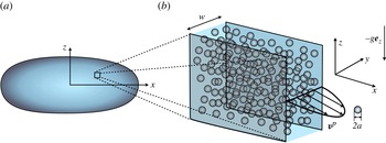
is the coordinate across the fracture, as shown in figure 1.
Schematics of (a) the hydraulic fracture and (b) the slurry flow inside it.

Assuming a steady flow, the governing equations (2.1) and (2.4) can be reduced to
 $$\begin{eqnarray}\displaystyle \boldsymbol{{\rm\nabla}}\boldsymbol{\cdot }(\unicode[STIX]{x1D64C}\,p^{p}) & = & \displaystyle \frac{\partial }{\partial y}\left({\it\mu}^{p}({\it\phi})\frac{\partial \boldsymbol{v}^{p}}{\partial y}\right)+{\it\eta}({\it\phi}){\rm\Delta}\boldsymbol{v}-{\it\phi}({\it\rho}^{p}-{\it\rho}^{f})g\boldsymbol{e}_{z},\end{eqnarray}$$
 $$\begin{eqnarray}\displaystyle \boldsymbol{{\rm\nabla}}\widetilde{p^{\,f}} & = & \displaystyle {\it\mu}^{f}\frac{\partial ^{2}\boldsymbol{v}^{p}}{\partial y^{2}}+{\it\mu}^{f}\frac{\partial ^{2}{\rm\Delta}\boldsymbol{v}}{\partial y^{2}}-{\it\eta}({\it\phi}){\rm\Delta}\boldsymbol{v}+\langle {\it\phi}\rangle ({\it\rho}^{p}-{\it\rho}^{f})g\boldsymbol{e}_{z},\end{eqnarray}$$
 $\boldsymbol{{\rm\nabla}}=(\partial /\partial x,\partial /\partial z)$
, and vectors
 $\boldsymbol{v}^{p}$
and
 ${\rm\Delta}\boldsymbol{v}=\boldsymbol{v}^{f}-\boldsymbol{v}^{p}$
also have only
 $x$
and
 $z$
components,
 $\langle {\it\phi}\rangle$
denotes average particle concentration across the channel, while
 $$\begin{eqnarray}\widetilde{p^{\,f}}=p^{\,f}+({\it\rho}^{f}g+\langle {\it\phi}\rangle ({\it\rho}^{p}-{\it\rho}^{f})g)z\end{eqnarray}$$
is the pressure that accounts for hydrostatic pressure. The particle pressure and effective shear viscosity of the particles are given respectively by
 $$\begin{eqnarray}\displaystyle & \displaystyle p^{p}={\it\mu}^{f}\mathscr{A}({\it\phi})^{-2}\left|\frac{\partial \boldsymbol{v}^{p}}{\partial y}\right|, & \displaystyle\end{eqnarray}$$
 $$\begin{eqnarray}\displaystyle & \displaystyle {\it\mu}^{p}={\it\mu}^{f}\left(\frac{5}{2}{\it\phi}_{m}\mathscr{A}({\it\phi})+{\it\mu}_{1}+\frac{{\it\mu}_{2}-{\it\mu}_{1}}{1+I_{0}\mathscr{A}({\it\phi})^{-2}}\right)\mathscr{A}({\it\phi})^{-2},\quad \mathscr{A}({\it\phi})=\frac{{\it\phi}_{m}}{{\it\phi}}-1. & \displaystyle\end{eqnarray}$$
 $\widetilde{p^{\,f}}=\widetilde{p^{\,f}}(x,z)$
and
 $p^{p}=p^{p}(x,z)$
owing to the steady-state property of the flow.
Assumptions
To account for realistic values of the parameters and to simplify the problem, the following three assumptions are made.
-
(a) For a continuum constitutive model to apply, it is implicitly assumed that
 $2a\ll w$
.
-
(b) The particle pressure gradient is neglected. To justify this assumption, note that the characteristic length of the problem,
$L$
(i.e. the length of the fracture), can be safely assumed to be much bigger than the width of the fracture,
$w$
. For instance, in typical hydraulic fracturing geometries,
$w/L=O(10^{-3})$
or less. In this case, one can use (3.2) and (3.4) to obtain estimates for
$p^{\,f}$
and
$p^{p}$
as (3.6a,b )which leads to
$$\begin{eqnarray}\boldsymbol{{\rm\nabla}}\widetilde{p^{\,f}}=O({\it\mu}^{f}\boldsymbol{v}^{f}w^{-2}),\quad \boldsymbol{{\rm\nabla}}p^{p}=O({\it\mu}^{f}\boldsymbol{v}^{p}(Lw)^{-1}),\end{eqnarray}$$
$|\boldsymbol{{\rm\nabla}}p^{p}/\boldsymbol{{\rm\nabla}}p^{\,f}|=O(w/L)\ll 1$
, provided that
$\boldsymbol{v}^{f}=O(\boldsymbol{v}^{p})$
. This estimate shows that the pressure gradient associated with the particles has a negligible contribution to the momentum change of the mixture. Note that this is true only for
${\it\phi}\neq {\it\phi}_{m}$
. As soon as particles become packed, i.e.
${\it\phi}={\it\phi}_{m}$
, they may sustain notable pressures and the particle pressure may not be neglected. In addition, it should be noted that ignoring the particle pressure gradient leads to the fact that the values of
${\it\lambda}_{1}$
and
${\it\lambda}_{3}$
are no longer important, because the variation of particle pressure becomes relevant only across the channel i.e. in the direction that corresponds to
${\it\lambda}_{2}$
.
-
(c) There is no gravity force in the
$y$
direction, i.e. across the channel. The geometry of the hydraulic fracture is determined predominantly by confining stresses. For deep fractures, the vertical stress is typically higher than the horizontal stress, in which case the fracture propagates in a vertical plane, and thus the projection of gravity force on the
$y$
axis is zero.





3.2. Steady solution
To obtain a steady solution, it is noted that the problem under consideration, (3.1)–(3.2), features a length scale
 $a\ll w$
, which causes the presence of a boundary layer with width
 $O(a)$
. The analysis of the boundary layer is very important, firstly to obtain a complete understanding of the problem, and secondly to obtain an accurate description of the slurry flow for all particle concentrations. This is particularly important for particle concentrations that are close to
 ${\it\phi}_{m}$
, as will be shown later. Let us focus first on the outer solution, i.e. the one that is valid away from the channel walls. In this situation, the term with the second derivative of
 ${\rm\Delta}\boldsymbol{v}$
in (3.2) can be neglected. Indeed, when the
 $y$
coordinate scales with
 $w$
, one can estimate
 $$\begin{eqnarray}\frac{\partial }{\partial y}\left({\it\mu}^{f}\frac{\partial {\rm\Delta}\boldsymbol{v}}{\partial y}\right)=O\left(\frac{{\it\mu}^{f}{\rm\Delta}\boldsymbol{v}}{w^{2}}\right),\quad {\it\eta}({\it\phi}){\rm\Delta}\boldsymbol{v}=O\left(\frac{{\it\phi}{\it\mu}^{f}{\rm\Delta}\boldsymbol{v}}{a^{2}}\right),\end{eqnarray}$$
so that the term with the second derivative of
 ${\rm\Delta}\boldsymbol{v}$
can be neglected as soon as
 $a^{2}/({\it\phi}w^{2})\ll 1$
. In situations when
 ${\it\phi}=O(a^{2}/w^{2})\ll 1$
, the viscosity associated with proppant is
 ${\it\mu}^{p}({\it\phi})=O({\it\phi})\ll 1$
, which makes the proppant contribution to the slurry flow negligible and leads to a well-known parabolic velocity profile. The fact that the term with the derivative of
 ${\rm\Delta}\boldsymbol{v}$
can be neglected should not be confused with the assumption of smallness of
 $|{\rm\Delta}\boldsymbol{v}/\boldsymbol{v}^{p}|$
. For relatively small particle concentrations, indeed
 $|{\rm\Delta}\boldsymbol{v}/\boldsymbol{v}^{p}|=O(a^{2}/w^{2})\ll 1$
, while higher concentrations (
 ${\it\phi}\approx {\it\phi}_{m}$
) may lead to
 $|{\rm\Delta}\boldsymbol{v}/\boldsymbol{v}^{p}|=O({\it\mu}_{1}{\it\phi}^{2}a^{2}/(w^{2}({\it\phi}_{m}-{\it\phi})^{2}))=O(1)$
, or even
 $\boldsymbol{v}^{p}=0$
for
 ${\it\phi}={\it\phi}_{m}$
. As was mentioned before, the term with the derivative of
 ${\rm\Delta}\boldsymbol{v}$
can be neglected away from the boundary, but at distances
 $O(a)$
from the boundary (i.e. in the boundary layer where the
 $y$
coordinate scales with
 $a$
), this term may have a significant contribution. As a result of the presence of the boundary layer, neither
 $\boldsymbol{v}^{p}$
nor
 ${\rm\Delta}\boldsymbol{v}$
(calculated for the outer solution) should satisfy a no-slip boundary condition at the channel walls. Instead,
 ${\rm\Delta}\boldsymbol{v}$
should approach some constant, while
 $\boldsymbol{v}^{p}$
should approach another constant, whose magnitude is
 $O({\rm\Delta}\boldsymbol{v})$
. Naturally, these constants should arise from the solution of the boundary layer problem.
By neglecting the particle pressure gradient and the second derivative of
 ${\rm\Delta}\boldsymbol{v}$
in (3.2), integrating the sum of the resultant equations and using (3.5), one can write
 $$\begin{eqnarray}\displaystyle & \displaystyle \boldsymbol{{\rm\nabla}}\widetilde{p^{\,f}}(y-y_{0})+({\it\rho}^{p}-{\it\rho}^{f})g\boldsymbol{e}_{z}\int _{y_{0}}^{y}({\it\phi}-\langle {\it\phi}\rangle )\,\text{d}\bar{y} & \displaystyle \nonumber\\ \displaystyle & \displaystyle \qquad =({\it\mu}^{f}+{\it\mu}^{p}({\it\phi}))\frac{\partial \boldsymbol{v}^{p}}{\partial y}-{\it\tau}(y_{0}),\quad y_{0}<y\leqslant {\textstyle \frac{1}{2}}w, & \displaystyle\end{eqnarray}$$
 $$\begin{eqnarray}\displaystyle & \displaystyle [\boldsymbol{{\rm\nabla}}\widetilde{p^{\,f}}+({\it\phi}_{m}-\langle {\it\phi}\rangle )({\it\rho}^{p}-{\it\rho}^{f})g\boldsymbol{e}_{z}]y={\it\tau},\quad |{\it\tau}|\leqslant {\it\mu}_{1}p^{p},\ \ 0\leqslant y\leqslant y_{0}, & \displaystyle\end{eqnarray}$$
 ${\it\tau}$
denotes shear stress. Here, only the solution for
 $y\geqslant 0$
is considered, owing to symmetry considerations. As indicated in the solution (3.8)–(3.9), there is a region with ‘no failure’ (
 $0\leqslant y\leqslant y_{0}$
), i.e. where the particles form a rigid cluster, and a region with shear motion or failure (
 $y_{0}<y\leqslant {\textstyle \frac{1}{2}}w$
). To find the particle pressure, one needs to evaluate (3.9) at
 $y=y_{0}$
, add the result to (3.8) evaluated at
 $y=w/2$
and use (3.4) to obtain
 $$\begin{eqnarray}p^{p}=\frac{w{\it\mu}^{f}|\boldsymbol{{\rm\nabla}}\widetilde{p^{\,f}}|}{2({\it\mu}^{f}+{\it\mu}^{p}({\it\phi}_{w}))\mathscr{A}({\it\phi}_{w})^{2}},\end{eqnarray}$$
where
 ${\it\phi}_{w}={\it\phi}|_{y=w/2}$
is the particle concentration at the wall. Since
 $|{\it\tau}|={\it\mu}_{1}p^{p}$
at the plug boundary, equations (3.10) and (3.9) can be used to calculate the plug size as
 $$\begin{eqnarray}y_{0}=\frac{w}{2}\frac{{\it\mu}_{1}[1+({\it\phi}_{m}/\langle {\it\phi}\rangle -1)^{2}G_{{\it\rho}}^{2}+2({\it\phi}_{m}/\langle {\it\phi}\rangle -1)G_{{\it\rho}}\cos {\it\psi}]^{-1/2}}{(1+{\it\mu}^{p}({\it\phi}_{w})/{\it\mu}^{f})\mathscr{A}({\it\phi}_{w})^{2}},\end{eqnarray}$$
where
 $$\begin{eqnarray}G_{{\it\rho}}=\frac{({\it\rho}^{p}-{\it\rho}^{f})g\langle {\it\phi}\rangle }{|\boldsymbol{{\rm\nabla}}\widetilde{p^{\,f}}|}\quad \text{and}\quad \cos {\it\psi}=|\boldsymbol{{\rm\nabla}}\widetilde{p^{\,f}}|^{-1}\frac{\partial \widetilde{p^{\,f}}}{\partial z}\end{eqnarray}$$
are two dimensionless parameters that represent the ratio between the gravitational force and pressure gradient, and the angle between the pressure gradient and the vertical
 $z$
axis, respectively. To find a solution for the particle concentration
 ${\it\phi}$
, it is useful to rewrite (3.1) using (3.4) and (3.10) as
 $$\begin{eqnarray}\displaystyle & & \displaystyle \left[\left(\frac{2y}{w}\right)^{2}+4G_{{\it\rho}}^{2}\left[\int _{0}^{y/w}({\it\phi}/\langle {\it\phi}\rangle -1)\,\text{d}s\right]^{2}+\frac{8y}{w}G_{{\it\rho}}\cos {\it\psi}\int _{0}^{y/w}({\it\phi}/\langle {\it\phi}\rangle -1)\,\text{d}s\right]^{1/2}\nonumber\\ \displaystyle & & \displaystyle \quad =\frac{({\it\mu}^{f}+{\it\mu}^{p}({\it\phi}))\mathscr{A}({\it\phi})^{2}}{({\it\mu}^{f}+{\it\mu}^{p}({\it\phi}_{w}))\mathscr{A}({\it\phi}_{w})^{2}},\end{eqnarray}$$
where
 $y_{0}<y\leqslant {\textstyle \frac{1}{2}}w$
. Given the values of
 $G_{{\it\rho}}$
,
 $\cos {\it\psi}$
and
 ${\it\phi}_{w}$
,
 ${\it\phi}$
can be determined by solving (3.13) numerically via Newton’s method. In this case the solution can be written in the form
 ${\it\phi}(s,{\it\phi}_{w},G_{{\it\rho}},\cos {\it\psi})$
or
 ${\it\phi}(s,\langle {\it\phi}\rangle ,G_{{\it\rho}},\cos {\it\psi})$
, where
 $s=y/w$
.
It is interesting to comment on the existence of a solution of (3.13). Unfortunately, (3.13) does not always have a solution. A thorough analysis of the existence of the solution is beyond the scope of this study. For this reason, let us focus on the simple case when
 $\cos {\it\psi}=-1$
. In this situation, the left-hand side of (3.13) is proportional to the absolute value of the function
 $h(y)=1-(wG_{{\it\rho}}/y)\int _{0}^{y/w}({\it\phi}/\langle {\it\phi}\rangle -1)\text{d}s$
. This function
 $h(y)$
is equal to
 $h(y_{0})=1-G_{{\it\rho}}({\it\phi}_{m}/\langle {\it\phi}\rangle -1)$
at the plug boundary, while
 $h(w/2)=1$
at the wall. If
 $h(y_{0})<0$
, then at some point
 $y_{0}<y_{\ast }<w/2$
this function vanishes (provided that it is continuous). However, the right-hand side of (3.13) cannot vanish, since its minimum value is
 ${\it\mu}_{1}{\it\mu}^{f}/[({\it\mu}^{f}+{\it\mu}^{p}({\it\phi}_{w}))\mathscr{A}({\it\phi}_{w})^{2}]>0$
. In this case, the necessary condition for the existence of a solution is
 $1-G_{{\it\rho}}({\it\phi}_{m}/\langle {\it\phi}\rangle -1)>0$
. This condition bounds the pressure gradient as
 $$\begin{eqnarray}-\frac{\partial \widetilde{p^{\,f}}}{\partial z}>({\it\rho}^{p}-{\it\rho}^{f})g({\it\phi}_{m}-\langle {\it\phi}\rangle ).\end{eqnarray}$$
Note that
 $\partial \widetilde{p^{\,f}}/\partial x=0$
and
 $-\partial \widetilde{p^{\,f}}/\partial z>0$
since
 $\cos {\it\psi}=-1$
, in which case the range over which the steady solution does not exist (according to (3.14)) is relatively narrow. It is also possible to explain why there is no steady solution. First, if
 $-\partial \widetilde{p^{\,f}}/\partial z>0$
, the slurry should flow in the positive
 $z$
direction since the average of the corresponding gravity term in the sum of (3.1) and (3.2) is zero. Since the shear stress is zero at the centre of the channel, the particles tend to form a plug. If the plug is formed, then, if (3.14) is not satisfied, the plug starts to sink as the pressure gradient is not sufficient to sustain it. If the plug sinks (i.e. flows in the negative
 $z$
direction), and the average velocity is positive, then, since the shear stress should be continuous, there is a point at which the shear stress is zero (as its sign is different at the wall and the boundary of the plug). If the shear stress is zero, then the particle pressure is zero as well (or there is another plug, which, if it exists, would sink too and cause a similar problem). Since there is some particle pressure at the central plug (otherwise, it would not form) and this pressure vanishes somewhere outside of it, then there is a particle pressure gradient, which moves particles away from the plug. As soon as particles move away and the concentration in the plug reduces, the particle pressure at the centre becomes zero (since the shear stress is zero due to symmetry), and this generates an opposite particle pressure gradient, which tends to form a plug again. This cyclic process repeats, so no steady solution exists in this case. Also note that a zero shear rate or a zero particle pressure at a point creates basic problems in the description (i.e. the model breaks down), which can be overcome by introducing some non-local description, as is shown in Nott & Brady (Reference Nott and Brady1994).
To find the outer solution (i.e. outside of the boundary layer) for the particle velocity, (3.8) can be integrated as
 $$\begin{eqnarray}\displaystyle \boldsymbol{v}^{p} & = & \displaystyle \boldsymbol{v}^{p}|_{y=w/2}+\boldsymbol{v}_{0}^{p}\nonumber\\ \displaystyle & = & \displaystyle \boldsymbol{v}^{p}|_{y=w/2}-\frac{w^{2}\boldsymbol{{\rm\nabla}}\widetilde{p^{\,f}}}{{\it\mu}^{f}}\int _{{\hat{s}}}^{1/2}\frac{\bar{s}\,\text{d}\bar{s}}{1+{\it\mu}^{p}({\it\phi}(\bar{s}))/{\it\mu}^{f}}\nonumber\\ \displaystyle & & \displaystyle -\,\frac{w^{2}({\it\rho}^{p}-{\it\rho}^{f})g\boldsymbol{e}_{z}}{{\it\mu}^{f}}\int _{{\hat{s}}}^{1/2}\frac{1}{1+{\it\mu}^{p}({\it\phi}(\bar{s}))/{\it\mu}^{f}}\int _{0}^{\bar{s}}({\it\phi}(s)-\langle {\it\phi}\rangle )\text{d}s\text{d}\bar{s},\end{eqnarray}$$
 ${\hat{s}}=\max \{y_{0}/w,y/w\}$
,
 $\boldsymbol{v}_{0}^{p}$
is the solution that satisfies the no-slip condition at the boundary, while
 $\boldsymbol{v}^{p}|_{y=w/2}$
is the integration constant that comes from the solution of the boundary layer problem. The slip velocity for the outer solution can be found from (3.1) and using (3.8) as
 $$\begin{eqnarray}{\rm\Delta}\boldsymbol{v}=-\frac{\boldsymbol{{\rm\nabla}}\widetilde{p^{\,f}}}{{\it\eta}({\it\phi})}\frac{\partial }{\partial s}\left(\frac{{\it\mu}^{p}({\it\phi})s}{{\it\mu}^{f}+{\it\mu}^{p}({\it\phi})}\right)+\frac{({\it\rho}^{p}-{\it\rho}^{f})g\boldsymbol{e}_{z}}{{\it\eta}({\it\phi})}\frac{\partial }{\partial s}\left(\frac{{\it\mu}^{f}\displaystyle \int _{0}^{s}{\it\phi}\,\text{d}\bar{s}}{{\it\mu}^{f}+{\it\mu}^{p}({\it\phi})}+\frac{{\it\mu}^{p}({\it\phi})\langle {\it\phi}\rangle s}{{\it\mu}^{f}+{\it\mu}^{p}({\it\phi})}\right),\end{eqnarray}$$
where
 $s=y/w$
is the scaled
 $y$
coordinate.
To find the inner or boundary layer solution, it is useful to represent the ‘full’ solution as the sum of the outer and the inner, so that
 ${\it\phi}^{F}={\it\phi}+{\it\delta}{\it\phi}$
,
 ${\rm\Delta}\boldsymbol{v}^{F}={\rm\Delta}\boldsymbol{v}+{\it\delta}{\rm\Delta}\boldsymbol{v}$
and
 $\boldsymbol{v}^{p,F}=\boldsymbol{v}_{0}^{p}+{\it\delta}\boldsymbol{v}^{p}$
. By substituting the above expressions into (3.1), (3.2) and (3.4) and using a Taylor series expansion, one finds that
 $$\begin{eqnarray}\displaystyle & \displaystyle \left.\frac{\partial {\it\mu}^{p}}{\partial {\it\phi}}\right|_{w}\left.\frac{\partial \boldsymbol{v}^{p}}{\partial y}\right|_{w}\frac{\partial {\it\delta}{\it\phi}}{\partial y}+{\it\mu}^{p}({\it\phi}_{w})\frac{\partial ^{2}{\it\delta}\boldsymbol{v}^{p}}{\partial y^{2}}+{\it\eta}({\it\phi}_{w}){\it\delta}{\rm\Delta}\boldsymbol{v}=0, & \displaystyle\end{eqnarray}$$
 $$\begin{eqnarray}\displaystyle & \displaystyle {\it\mu}^{f}\frac{\partial ^{2}{\it\delta}\boldsymbol{v}^{p}}{\partial y^{2}}+{\it\mu}^{f}\frac{\partial ^{2}{\it\delta}{\rm\Delta}\boldsymbol{v}}{\partial y^{2}}-{\it\eta}({\it\phi}_{w}){\it\delta}{\rm\Delta}\boldsymbol{v}=0, & \displaystyle\end{eqnarray}$$
 $$\begin{eqnarray}\displaystyle & \displaystyle \left|\left.\frac{\partial \boldsymbol{v}^{p}}{\partial y}\right|_{w}\right|^{-2}\left(\frac{\partial {\it\delta}\boldsymbol{v}^{p}}{\partial y}\boldsymbol{\cdot }\left.\frac{\partial \boldsymbol{v}^{p}}{\partial y}\right|_{w}\right)=\frac{2}{\mathscr{A}({\it\phi}_{w})}\left.\frac{\partial \mathscr{A}}{\partial {\it\phi}}\right|_{w}{\it\delta}{\it\phi}, & \displaystyle\end{eqnarray}$$
 $|_{w}$
’ means evaluation of the outer solution at the wall. Note that, since
 $y=O(a)$
and
 $|{\rm\Delta}\boldsymbol{v}/\boldsymbol{v}^{p}|=O(a^{2}/w^{2})$
for the inner solution (
 $y=O(w)$
for the outer solution), it can be concluded that
 ${\it\delta}{\it\phi}=O(a/w)\ll 1$
,
 ${\it\delta}\boldsymbol{v}^{p}=O({\rm\Delta}\boldsymbol{v})\ll \boldsymbol{v}^{p}$
, which validates the use of a Taylor series expansion. At the same time,
 ${\it\delta}{\rm\Delta}\boldsymbol{v}=O({\rm\Delta}\boldsymbol{v})$
, but no expansion has been used with
 ${\rm\Delta}\boldsymbol{v}$
. The solution of the above system of equations (3.17)–(3.19), which accounts for both the no-slip boundary conditions and the far-field behaviour, is
 $$\begin{eqnarray}\displaystyle \displaystyle {\it\delta}{\rm\Delta}\boldsymbol{v} & = & \displaystyle -V_{1}\text{e}^{-{\it\gamma}_{1}y}-V_{2}\text{e}^{-{\it\gamma}_{2}y},\end{eqnarray}$$
 $$\begin{eqnarray}\displaystyle \displaystyle {\it\delta}\boldsymbol{v}^{p} & = & \displaystyle C_{1}V_{1}(1-\text{e}^{-{\it\gamma}_{1}y})+C_{2}V_{2}(1-\text{e}^{-{\it\gamma}_{2}y}),\end{eqnarray}$$
 $$\begin{eqnarray}\displaystyle \displaystyle {\it\delta}{\it\phi} & = & \displaystyle C_{3}\text{e}^{-{\it\gamma}_{1}y},\end{eqnarray}$$
 $$\begin{eqnarray}V_{1}=\left|\left.\frac{\partial \boldsymbol{v}^{p}}{\partial y}\right|_{w}\right|^{-2}\left({\rm\Delta}\boldsymbol{v}|_{w}\boldsymbol{\cdot }\left.\frac{\partial \boldsymbol{v}^{p}}{\partial y}\right|_{w}\right)\left.\frac{\partial \boldsymbol{v}^{p}}{\partial y}\right|_{w},\quad V_{2}={\rm\Delta}\boldsymbol{v}|_{w}-V_{1},\end{eqnarray}$$
 $$\begin{eqnarray}{\it\gamma}_{1}=\left(\frac{{\it\eta}({\it\phi}_{w})}{{\it\mu}^{f}(1-\mathscr{B}({\it\phi}_{w}))}\right)^{1/2},\quad {\it\gamma}_{2}=\left(\frac{{\it\eta}({\it\phi}_{w})}{{\it\mu}^{f}}\left(1+\frac{{\it\mu}^{f}}{{\it\mu}^{p}({\it\phi}_{w})}\right)\right)^{1/2},\end{eqnarray}$$
 $$\begin{eqnarray}C_{1}=-\mathscr{B}({\it\phi}_{w}),\quad C_{2}=-\frac{{\it\mu}^{f}}{{\it\mu}^{f}+{\it\mu}^{p}({\it\phi}_{w})},\end{eqnarray}$$
 $$\begin{eqnarray}C_{3}=\mathscr{B}({\it\phi}_{w})\left(\frac{{\it\eta}({\it\phi}_{w})}{{\it\mu}^{f}(1-\mathscr{B}({\it\phi}_{w}))}\right)^{1/2}\left|\left.\frac{\partial \boldsymbol{v}^{p}}{\partial y}\right|_{w}\right|^{-2}\left({\rm\Delta}\boldsymbol{v}|_{w}\boldsymbol{\cdot }\left.\frac{\partial \boldsymbol{v}^{p}}{\partial y}\right|_{w}\right)\frac{\mathscr{A}({\it\phi}_{w}){\it\phi}_{w}^{2}}{2{\it\phi}_{m}},\end{eqnarray}$$
and the auxiliary function
 $\mathscr{B}({\it\phi})$
is
 $$\begin{eqnarray}\mathscr{B}({\it\phi})=2\mathscr{A}({\it\phi})\left[2\mathscr{A}({\it\phi})+\frac{5}{2}{\it\phi}_{m}+\frac{2({\it\mu}_{2}-{\it\mu}_{1})I_{0}\mathscr{A}({\it\phi})}{(I_{0}+\mathscr{A}({\it\phi})^{2})^{2}}\right]^{-1}.\end{eqnarray}$$
Note that
 ${\rm\Delta}\boldsymbol{v}^{F}={\rm\Delta}\boldsymbol{v}+{\it\delta}{\rm\Delta}\boldsymbol{v}$
satisfies the no-slip boundary condition since
 $V_{1}+V_{2}={\rm\Delta}\boldsymbol{v}|_{w}$
. The ‘full’ solution for the particle velocity
 $\boldsymbol{v}^{p,F}=\boldsymbol{v}_{0}^{p}+{\it\delta}\boldsymbol{v}^{p}$
satisfies the no-slip boundary condition as well. To find
 $\boldsymbol{v}_{x}^{p}|_{y=w/2}$
featured in (3.15), one needs to take a limit in (3.21) to find
 $$\begin{eqnarray}\boldsymbol{v}^{p}|_{y=w/2}=C_{1}V_{1}+C_{2}V_{2}.\end{eqnarray}$$
Since
 $C_{1}({\it\phi}_{w}=0)=C_{2}({\it\phi}_{w}=0)=-1$
and
 $C_{1}({\it\phi}_{w}={\it\phi}_{m})=C_{2}({\it\phi}_{w}={\it\phi}_{m})=0$
, (3.28) implies that
 $\boldsymbol{v}^{f}|_{y=w/2}=0$
for zero proppant concentration and
 $\boldsymbol{v}^{p}|_{y=w/2}=0$
for the maximum proppant concentration. Indeed, if there are no particles, the fluid velocity (outer solution) should satisfy a no-slip boundary condition. At the same time, the maximum particle concentration corresponds to a rigid plug, which does not move, so that the particle velocity (outer solution) should satisfy a no-slip condition at the boundary. It is also important to note that the values of
 ${\it\gamma}_{1}$
and
 ${\it\gamma}_{2}$
are always
 $O(1/a)$
, and in the limit of small particle concentrations they reach finite values
 ${\it\gamma}_{1}\approx \sqrt{18/5}\,a^{-1}$
and
 ${\it\gamma}_{2}\approx \sqrt{9/5}\,a^{-1}$
. Equation (3.28) is the main outcome of the analysis of the boundary layer. It is responsible for the boundary condition, which effectively describes transition between Poiseuille flow at low particle concentrations and Darcy’s law for high particle concentrations. Avoiding the analysis of the boundary layer can lead to inaccurate behaviour at higher concentrations, while the behaviour at small concentrations is, practically, not affected.
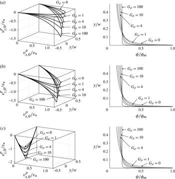
Normalized particle velocity profile and normalized particle volume fraction versus
 $y/w$
for
 $G_{{\it\rho}}=\{0,1,4,10,100\}$
and
 $\langle {\it\phi}\rangle =0.2\times {\it\phi}_{m}$
, (a)
 $\cos {\it\psi}=0$
, (b)
 $\cos {\it\psi}=1/2$
, (c)
 $\cos {\it\psi}=1$
.

To visualize the solution, figure 2 shows the velocity profile
 $\boldsymbol{v}_{0}^{p}$
(calculated numerically), normalized by
 $v_{\ast }=(12{\it\mu}^{f})^{-1}w^{2}|\boldsymbol{{\rm\nabla}}\widetilde{p^{\,f}}|$
and the proppant concentration variation (calculated numerically), normalized by
 ${\it\phi}_{m}$
, for different values of the parameter
 $G_{{\it\rho}}=\{0,1,4,10,100\}$
, and for different values of
 $\cos {\it\psi}=\{0,1/2,1\}$
, while the average proppant concentration is kept fixed,
 $\bar{{\it\phi}}=\langle {\it\phi}\rangle /{\it\phi}_{m}=0.2$
. As can be seen from the figure, the presence of the gravitational force leads to a redistribution of the particles across the channel. Moreover, the value of
 $\cos {\it\psi}$
has a small impact on the particle distribution. In the limiting case when
 $G_{{\it\rho}}\gg 1$
, the particles are distributed uniformly everywhere except for the narrow region at the centre (which corresponds to the plug). For
 $\cos {\it\psi}=1$
and
 $G_{{\it\rho}}=100$
, the velocity profile resembles a wedge. This strange velocity profile can be explained by the fact that the forcing term for the sum of equations (3.1) and (3.2) behaves like a delta function for
 $G_{{\it\rho}}\gg 1$
, i.e.
 $(\partial \widetilde{p^{\,f}}/\partial z)(1+G_{{\it\rho}}({\it\phi}/\langle {\it\phi}\rangle -1))\rightarrow (\partial \widetilde{p^{\,f}}/\partial z)\,w{\it\delta}(y)$
, where
 ${\it\delta}(y)$
denotes the Dirac delta function. This delta-function-like pressure gradient distribution leads to the wedge-like velocity profile.
3.3. Approximate steady solution
Numerical solution of (3.13) together with (3.11), (3.15), (3.16) and (3.28) give a complete solution for the problem. Unfortunately, this solution relies on the numerical evaluation of the function
 ${\it\phi}(s,\langle {\it\phi}\rangle ,G_{{\it\rho}},\cos {\it\psi})$
, which depends on many parameters and thus is hard to tabulate for the purpose of implementing into a hydraulic fracturing simulator. Moreover, as noted in the previous section, a steady solution does not exist for all ranges of parameters. For these reasons, it is more practicable to introduce an approximate solution, which would simplify (3.13) and lead to a solution that can be implemented into a hydraulic fracturing simulator. The ‘full’ solution can then be used to estimate the error in the approximation.
Clearly, if there is no gravity (i.e.
 $g=0$
and consequently
 $G_{{\it\rho}}=0$
), (3.13) becomes an algebraic equation that is easy to solve. Unfortunately, the absence of gravity not only leads to a simplified slurry flow, but the model also loses the ability to capture gravitational settling of particles. However, the latter phenomenon is very important and needs to be accounted for at least approximately. To motivate the approximation that we are about to make, we observe from the plots of
 ${\it\phi}/{\it\phi}_{m}$
in figure 2 that the proppant distribution does not change appreciably as
 $G_{{\it\rho}}$
is varied (except for
 $G_{{\it\rho}}=100$
) or as
 $\cos {\it\psi}$
varies from 0 to 1. Thus to simplify the solution and to keep the gravitational settling at the same time, it is assumed that gravity does not affect the particle distribution, i.e. terms with
 $G_{{\it\rho}}$
can be neglected in (3.8) and (3.9). In other words, the solution for
 ${\it\phi}$
is approximated by
 $$\begin{eqnarray}{\it\phi}(s,\langle {\it\phi}\rangle ,G_{{\it\rho}},\cos {\it\psi})\approx {\it\phi}(s,\langle {\it\phi}\rangle ,0,0),\end{eqnarray}$$
where
 $s=y/w$
. Note that this assumption is equivalent to replacing
 $\langle {\it\phi}\rangle$
by
 ${\it\phi}$
in the gravity term in (3.2), instead of neglecting the whole gravity term when gravity is assumed to be negligible. As a result, the gravity term that causes the gravitational settling is still accounted for, but in an approximate fashion. In terms of the error, there are two main quantities that are important for hydraulic fracturing, namely the slurry flux and the proppant flux. For the cases considered in figure 2, i.e.
 $G_{{\it\rho}}=\{1,4,10,100\}$
, the corresponding error (relative to the
 $G_{{\it\rho}}=0$
solution) in terms of the absolute value of the slurry flux and the particle flux is
 $e^{s}=\{0.02,0.01,0.03,0.14\}$
and
 $e^{p}=\{0.04,0.07,0.06,0.01\}$
for
 $\cos {\it\psi}=0$
,
 $e^{s}=\{0.03,0.11,0.18,0.24\}$
and
 $e^{p}=\{0.005,0.04,0.08,0.09\}$
for
 $\cos {\it\psi}=1/2$
, and
 $e^{s}=\{0.07,0.20,0.29,0.29\}$
and
 $e^{p}=\{0.06,0.15,0.20,0.15\}$
for
 $\cos {\it\psi}=1$
. Here the slurry flux is calculated as an integral of
 $\boldsymbol{v}_{0}^{p}$
, while the particle flux is calculated as an integral of
 ${\it\phi}\boldsymbol{v}_{0}^{p}$
. This shows that, even in the worst case of
 $G_{{\it\rho}}=100$
, the flux error is less than 30 %. Also, there is an error in the direction of the flux, but the direction can be corrected by the presence of an extra hydrostatic pressure gradient inside the fracture. So the error in the direction of the flow affects the hydrostatic pressure inside the fracture. Note that, for other average particle concentrations, the order of magnitude of the error does not change appreciably. For instance, for
 $\bar{{\it\phi}}=\langle {\it\phi}\rangle /{\it\phi}_{m}=0.5$
, the corresponding errors are
 $e^{s}=\{0.03,0.11,0.14,0.16\}$
and
 $e^{p}=\{0.04,0.13,0.19,0.23\}$
for
 $\cos {\it\psi}=0$
,
 $e^{s}=\{0.01,0.02,0.03,0.09\}$
and
 $e^{p}=\{0.02,0.05,0.07,0.17\}$
for
 $\cos {\it\psi}=1/2$
, and
 $e^{s}=\{0.02,0.06,0.08,0.01\}$
and
 $e^{p}=\{0.02,0.06,0.06,0.04\}$
for
 $\cos {\it\psi}=1$
.
To estimate the error distribution over the fracture, it is useful to provide an estimate for the parameter
 $G_{{\it\rho}}$
. One may calculate the pressure gradient as
 $|\boldsymbol{{\rm\nabla}}\widetilde{p^{\,f}}|=12{\it\mu}^{f}|\boldsymbol{V}|/w^{2}$
, where
 ${\it\mu}^{f}$
is the intrinsic fluid viscosity,
 $w$
is the width of the channel and
 $\boldsymbol{V}$
is the average fluid velocity. By taking
 ${\it\mu}^{f}=0.1\ \text{Pa}\ \text{s}$
,
 $w=1\ \text{cm}$
,
 $\langle {\it\phi}\rangle =0.1$
,
 ${\it\rho}^{p}-{\it\rho}^{f}=1300\ \text{kg}\ \text{m}^{-3}$
and
 $|\boldsymbol{V}|=0.1\ \text{m}\ \text{s}^{-1}$
, one may estimate
 $G_{{\it\rho}}$
as
 $$\begin{eqnarray}G_{{\it\rho}}=\frac{\langle {\it\phi}\rangle ({\it\rho}^{p}-{\it\rho}^{f})gw^{2}}{12{\it\mu}^{f}|\boldsymbol{V}|}\approx 1,\end{eqnarray}$$
which shows that the effect of gravity is relatively small for the considered parameters. However,
 $G_{{\it\rho}}$
might increase noticeably for wider and slower fractures. Typically, hydraulic fractures are narrow and propagate rapidly at early stages, while they become wider and slow down later in their evolution. In this case, it is important to monitor the criterion (3.30) for mature fractures. Note that, for a better estimate, one needs to insert the effective viscosity in (3.30), which further decreases the value of
 $G_{{\it\rho}}$
. Also note that both the fracture width
 $w$
and the average fluid velocity
 $\boldsymbol{V}$
reach their respective maxima at the well bore (the velocity is singular if a point source is used). In this case, the parameter
 $G_{{\it\rho}}$
reaches its maximum some distance away from the well bore, and is negligible near the well bore and near the crack tip. Given the fact that the parameter
 $G_{{\it\rho}}$
may vary significantly over the fracture and may cause a relatively small error only in a localized region, the solution (3.29) can be used throughout the fracture as an adequately accurate approximation.
Using the approximation (3.29) and (3.10), (3.13) can be inverted to find
 $$\begin{eqnarray}\mathscr{A}({\it\phi})=F\left(|\boldsymbol{{\rm\nabla}}\widetilde{p^{\,f}}|\,\frac{y-y_{0}}{p^{p}}\right),\end{eqnarray}$$
where
 $F$
is a function that can be calculated numerically (or evaluated using the formula for the roots of a fourth-degree polynomial). For future reference it is noted that the asymptotic behaviour of the function
 $F$
is
 $$\begin{eqnarray}F(s)\mathop{=}\limits^{s\rightarrow 0}F_{0}(s)=\frac{2s}{5{\it\phi}_{m}},\quad F(s)\mathop{=}\limits^{s\rightarrow \infty }F_{\infty }(s)=\sqrt{s}.\end{eqnarray}$$
Using the definition of
 $\mathscr{A}({\it\phi})$
from (3.5), one may express the particle concentration from (3.31) as
 $$\begin{eqnarray}\displaystyle & {\it\phi}(y)=\displaystyle \frac{{\it\phi}_{m}}{1+F\left(|\boldsymbol{{\rm\nabla}}\widetilde{p^{\,f}}|\,\displaystyle \frac{y-y_{0}}{p^{p}}\right)},\quad y_{0}<y\leqslant {\textstyle \frac{1}{2}}w, & \displaystyle\end{eqnarray}$$
 $$\begin{eqnarray}\displaystyle & \displaystyle {\it\phi}(y)={\it\phi}_{m},\quad 0\leqslant y\leqslant y_{0}. & \displaystyle\end{eqnarray}$$
 ${\it\phi}_{m}$
as
 $$\begin{eqnarray}\bar{{\it\phi}}=\frac{\langle {\it\phi}\rangle }{{\it\phi}_{m}}=\frac{2}{w}\int _{0}^{w/2}\frac{{\it\phi}(y)}{{\it\phi}_{m}}\,\text{d}y,\end{eqnarray}$$
so that
 $0\leqslant \bar{{\it\phi}}\leqslant 1$
. By inverting the latter relation, the particle pressure and the half-width of the rigid cluster zone can be computed as
 $$\begin{eqnarray}p^{p}=w|\boldsymbol{{\rm\nabla}}\widetilde{p^{\,f}}|\,{\it\Pi}(\bar{{\it\phi}}),\quad y_{0}={\it\mu}_{1}w{\it\Pi}(\bar{{\it\phi}}),\end{eqnarray}$$
where
 $G_{{\it\rho}}=0$
(or
 ${\it\phi}=\langle {\it\phi}\rangle$
) is used in (3.11) to calculate
 $y_{0}$
, and
 ${\it\Pi}(\bar{{\it\phi}})$
is a function that is evaluated numerically. Note that the asymptotic behaviour of the function
 ${\it\Pi}(\bar{{\it\phi}})$
for small and high average volume concentrations of particles is
 $$\begin{eqnarray}{\it\Pi}(\bar{{\it\phi}})\mathop{=}\limits^{\bar{{\it\phi}}\rightarrow 0}{\it\Pi}_{0}(\bar{{\it\phi}})={\textstyle \frac{1}{8}}\bar{{\it\phi}}^{2},\quad {\it\Pi}(\bar{{\it\phi}})\mathop{=}\limits^{\bar{{\it\phi}}\rightarrow 1}{\it\Pi}_{1}(\bar{{\it\phi}})=\frac{1}{2{\it\mu}_{1}}-\sqrt{\frac{5{\it\phi}_{m}(1-\bar{{\it\phi}})}{4{\it\mu}_{1}^{3}}}.\end{eqnarray}$$
Equation (3.36) allows us to replace the particle pressure
 $p^{p}$
by the normalized average volume fraction
 $\bar{{\it\phi}}$
, in which case (3.33) and (3.34) can be rewritten as
 $$\begin{eqnarray}{\it\phi}=\frac{{\it\phi}_{m}}{1+F\left(\max \left\{\displaystyle \frac{y/w}{{\it\Pi}(\bar{{\it\phi}})}-{\it\mu}_{1},\ 0\right\}\right)}.\end{eqnarray}$$
The function
 ${\it\Pi}(\bar{{\it\phi}})$
is directly related to the particle concentration at the wall through the relation
 $$\begin{eqnarray}{\it\phi}_{w}=\frac{{\it\phi}_{m}}{1+F\left(\displaystyle \frac{1}{2{\it\Pi}(\bar{{\it\phi}})}-{\it\mu}_{1}\right)},\end{eqnarray}$$
so that the above relation
 ${\it\phi}_{w}={\it\phi}_{w}(\bar{{\it\phi}})$
can be alternatively used instead of
 ${\it\Pi}(\bar{{\it\phi}})$
.
To find the velocity distribution, we integrate (3.4), use (3.36) and the fact that
 $\boldsymbol{v}_{0}^{p}\propto \boldsymbol{{\rm\nabla}}\widetilde{p^{\,f}}$
to obtain
 $$\begin{eqnarray}\boldsymbol{v}^{p}=\boldsymbol{v}^{p}|_{y=w/2}+\boldsymbol{v}_{0}^{p}=\boldsymbol{v}^{p}|_{y=w/2}-\frac{w^{2}{\it\Pi}(\bar{{\it\phi}})}{{\it\mu}^{f}}\boldsymbol{{\rm\nabla}}\widetilde{p^{\,f}}\int _{ max\{y/w,\,{\it\mu}_{1}{\it\Pi}(\bar{{\it\phi}})\}}^{1/2}\left[F\left(\frac{s}{{\it\Pi}(\bar{{\it\phi}})}-{\it\mu}_{1}\right)\right]^{2}\text{d}s.\end{eqnarray}$$
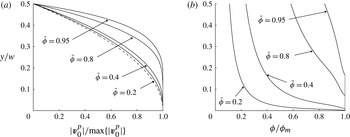
As an illustration, figure 3 shows the velocity profiles given by (3.40) and the corresponding particle concentration profiles, computed using (3.38) versus
 $y/w$
. Figure 3 clearly indicates the presence of the rigid zone; however, the size of this zone becomes more pronounced only for high values of
 $\bar{{\it\phi}}$
, i.e. high concentrations. Also note that the velocity profile deviates from a parabolic shape for higher
 $\bar{{\it\phi}}$
and has a blunted profile, which was also shown in Nott & Brady (Reference Nott and Brady1994) and Eskin & Miller (Reference Eskin and Miller2008).
(a) Normalized velocity of the slurry and (b) normalized particle volume fraction versus
 $y/w$
for different values of
 $\bar{{\it\phi}}=\{0.2,0.4,0.8,0.95\}$
. The dashed line in panel (a) indicates the parabolic profile associated with
 $\bar{{\it\phi}}=0$
.

To capture the difference between the fluid and particle velocities, the slip velocity can be deduced from (3.1), (3.4), (3.10), (3.13) and (3.16) as
 $$\begin{eqnarray}{\rm\Delta}\boldsymbol{v}=\boldsymbol{v}^{f}-\boldsymbol{v}^{p}=-\frac{1-\mathscr{B}({\it\phi})}{{\it\eta}({\it\phi})}\boldsymbol{{\rm\nabla}}\widetilde{p^{\,f}}+({\it\rho}^{p}-{\it\rho}^{f})g\boldsymbol{e}_{z}\frac{{\it\phi}}{{\it\eta}({\it\phi})},\end{eqnarray}$$
where
 ${\it\phi}={\it\phi}(y)$
is taken from (3.38) and
 $\mathscr{B}$
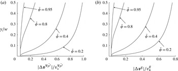
is given in (3.27). Figure 4 shows the normalized slip velocity for the case when
 $g=0$
, i.e.
 $|{\rm\Delta}\boldsymbol{v}^{\boldsymbol{{\rm\nabla}}\widetilde{p^{\,f}}}|/v_{\ast }^{\boldsymbol{{\rm\nabla}}\widetilde{p^{\,f}}}$
, and for the case when
 $\boldsymbol{{\rm\nabla}}\widetilde{p^{\,f}}=0$
, i.e.
 $|{\rm\Delta}\boldsymbol{v}^{g}|/v_{\ast }^{g}$
, versus
 $y/w$
for different values of
 $\bar{{\it\phi}}$
. The slip velocities are normalized respectively by
 $$\begin{eqnarray}v_{\ast }^{\boldsymbol{{\rm\nabla}}\widetilde{p^{\,f}}}=\frac{2a^{2}}{9{\it\mu}^{f}}|\boldsymbol{{\rm\nabla}}\widetilde{p^{\,f}}|,\quad v_{\ast }^{g}=\frac{2a^{2}}{9{\it\mu}^{f}}({\it\rho}^{p}-{\it\rho}^{f})g.\end{eqnarray}$$
As can be seen from the figure, the two slip velocities have qualitatively similar profiles, although their magnitudes are different.
(a) Normalized slip velocity due to the pressure gradient
 $|{\rm\Delta}\boldsymbol{v}^{\boldsymbol{{\rm\nabla}}\widetilde{p^{\,f}}}|/v_{\ast }^{\boldsymbol{{\rm\nabla}}\widetilde{p^{\,f}}}$
and (b) normalized settling velocity
 $|{\rm\Delta}\boldsymbol{v}^{g}|/v_{\ast }^{g}$
versus scaled
 $y/w$
coordinate for different values of
 $\bar{{\it\phi}}=\{0.2,0.4,0.8,0.95\}$
.

To find
 $\boldsymbol{v}^{p}|_{y=w/2}$
, one may simplify (3.28) using (3.41) to give
 $$\begin{eqnarray}\displaystyle \boldsymbol{v}^{p}|_{y=w/2} & = & \displaystyle -C_{1}\frac{1-\mathscr{B}({\it\phi}_{w})}{{\it\eta}({\it\phi}_{w})}\boldsymbol{{\rm\nabla}}\widetilde{p^{\,f}}+C_{2}({\it\rho}^{p}-{\it\rho}^{f})g\boldsymbol{e}_{z}\frac{{\it\phi}_{w}}{{\it\eta}({\it\phi}_{w})}\nonumber\\ \displaystyle & & \displaystyle +\,(C_{1}-C_{2})\frac{({\it\rho}^{p}-{\it\rho}^{f})g}{|\boldsymbol{{\rm\nabla}}\widetilde{p^{\,f}}|^{2}}\frac{\partial \widetilde{p^{\,f}}}{\partial z}\frac{{\it\phi}_{w}}{{\it\eta}({\it\phi}_{w})}\boldsymbol{{\rm\nabla}}\widetilde{p^{\,f}},\end{eqnarray}$$
 $C_{1}$
and
 $C_{2}$
are given in (3.25).
To summarize, the particle, fluid and slurry velocities are given respectively by
 $$\begin{eqnarray}\displaystyle \boldsymbol{v}^{p} & = & \displaystyle \displaystyle \boldsymbol{v}^{p}|_{y=w/2}+\boldsymbol{v}_{0}^{p},\end{eqnarray}$$
 $$\begin{eqnarray}\displaystyle \boldsymbol{v}^{f} & = & \displaystyle \displaystyle \boldsymbol{v}^{p}|_{y=w/2}+\boldsymbol{v}_{0}^{p}+{\rm\Delta}\boldsymbol{v},\end{eqnarray}$$
 $$\begin{eqnarray}\displaystyle \boldsymbol{v}^{s} & = & \displaystyle \displaystyle {\it\phi}\boldsymbol{v}^{p}+(1-{\it\phi})\boldsymbol{v}^{f}=\boldsymbol{v}^{p}|_{y=w/2}+\boldsymbol{v}_{0}^{p}+(1-{\it\phi}){\rm\Delta}\boldsymbol{v},\end{eqnarray}$$
 $\boldsymbol{v}^{p}|_{y=w/2}$
is given in (3.43),
 $\boldsymbol{v}_{0}^{p}$
stems from (3.40), while
 ${\rm\Delta}\boldsymbol{v}$
is calculated according to (3.41).
3.4. Estimation of the characteristic length to establish a steady flow
The governing equations adopted for this study open the possibility to estimate the characteristic length required to establish a steady flow, which is an alternative to (1.2). By using the current problem geometry, assuming that initially
 ${\it\phi}(y)=\text{const.}$
, and that the velocity profile is parabolic, i.e.
 $\boldsymbol{v}^{p}=6w^{-2}(w^{2}/4-y^{2})\langle \boldsymbol{v}^{p}\rangle$
, the
 $y$
component of the particle pressure gradient can be estimated from (3.4) as
 $$\begin{eqnarray}\frac{\partial p^{p}}{\partial y}=-{\it\mu}^{f}\mathscr{A}({\it\phi})^{-2}\frac{12|\langle \boldsymbol{v}^{p}\rangle |}{w^{2}},\end{eqnarray}$$
where
 $|\langle \boldsymbol{v}^{p}\rangle |$
is an average velocity of the flow. Using the previous equation together with (2.1), the
 $y$
component of the velocity of the particles can be found as
 $$\begin{eqnarray}\boldsymbol{v}_{y}^{p}=-\frac{8}{3}\frac{{\it\phi}(1-{\it\phi})^{\bar{{\it\alpha}}}}{({\it\phi}_{m}-{\it\phi})^{2}}\frac{a^{2}}{w^{2}}|\langle \boldsymbol{v}^{p}\rangle |.\end{eqnarray}$$
The characteristic time required to establish steady flow is
 $t^{\ast }=w/(2|\boldsymbol{v}_{y}^{p}|)$
, while the corresponding length is
 $L=|\langle \boldsymbol{v}^{p}\rangle |t^{\ast }$
, so that
 $$\begin{eqnarray}\frac{L}{w}=\frac{3}{16}\frac{({\it\phi}_{m}-{\it\phi})^{2}}{{\it\phi}(1-{\it\phi})^{\bar{{\it\alpha}}}}\,\frac{w^{2}}{a^{2}}.\end{eqnarray}$$
Relation (3.49) is in agreement with (1.2), compatible with the adopted model, and provides a more accurate estimate for different values of
 ${\it\phi}$
. As an example, for
 ${\it\phi}=0.1$
,
 $a=0.4\ \text{mm}$
and
 $w=1\ \text{cm}$
, the length required to establish a steady flow is approximately equal to 4 m. For this set of problem parameters, if the fracture is longer than 4 m (while the width is 1 cm), then the assumption of steady flow is appropriate.
3.5. Comparison to the model in Lecampion & Garagash (Reference Lecampion and Garagash2014)
It is interesting to compare the model for slurry flow in a channel, developed in this section, to that independently developed in Lecampion & Garagash (Reference Lecampion and Garagash2014), as these models are both based on the same empirical constitutive relations published in Boyer et al. (Reference Boyer, Guazzelli and Pouliquen2011). The main difference comes from the fact that the model in Lecampion & Garagash (Reference Lecampion and Garagash2014) neglects the slip velocity and gravitational settling at the outset, and uses a slightly modified constitutive model. However, the importance of including the slip velocity and performing the associated boundary layer analysis is twofold. Firstly, one obtains a more complete understanding of the problem. Secondly, the boundary layer analysis enables us to capture the complete transition from Poiseuille flow for low particle concentrations, for which the slip velocity is negligible, to Darcy’s law for high particle concentrations, for which slip velocity is a primary mechanism for fluid transport (i.e. filtration). If one neglected either the slip velocity or the boundary layer, Darcy’s law would not be recovered in the limiting case. The boundary layer analysis also highlights the appropriate boundary conditions for the outer (macroscopic) solution, which is used to construct the lubrication equations for hydraulic fracture modelling. The boundary conditions for the model in Lecampion & Garagash (Reference Lecampion and Garagash2014) are no-slip throughout for all values of
 ${\it\phi}$
. Our results show that a no-slip boundary condition is a good approximation for dilute suspensions without gravitational settling and before entering the infiltration limit, at which Darcy’s law applies. However, in the infiltration limit or with gravitational settling, a slip boundary condition is required for the outer solution. Therefore, our analysis highlights the applicability of the model in Lecampion & Garagash (Reference Lecampion and Garagash2014) and establishes its limitations in the filtration and settling regimes. Naturally, the results of Lecampion & Garagash (Reference Lecampion and Garagash2014) can be recovered if both gravity and slip velocity are neglected in the current approach. Despite the fact that the effect of gravity is simplified in our approximate solution, the rigorous introduction of the gravity force in the complete solution enabled us to obtain a reference solution, from which we estimated the level of applicability of our approximation.
4. Mass transport equations
The goal of this section is to connect the developments of § 3 to the hydraulic fracturing problem. To achieve this, the fracture is represented by a channel with a variable width
 $w(x,z,t)$
, and it is assumed that the flow at any point is always in equilibrium or in a steady-state condition. To formulate the governing equations for the mass transport in a one-dimensional setting, it is necessary to integrate (2.2) and (2.5) over
 $y$
from
 $-w/2$
to
 $w/2$
and to derive equations for averaged quantities (note that the coordinate system is the same as that assumed in § 3). By using symmetry, the relation (3.35) and noting that, for any function
 $h(t,s)$
, one has
 $$\begin{eqnarray}2\frac{\partial }{\partial t}\int _{0}^{w/2}h(t,s)\,\text{d}s=2\int _{0}^{w/2}\frac{\partial h(t,s)}{\partial t}\,\text{d}s+h(t,w/2)\frac{\partial w}{\partial t},\end{eqnarray}$$
equations (2.2) and (2.5) can be integrated to obtain
 $$\begin{eqnarray}\displaystyle \displaystyle \frac{\partial w}{\partial t}+\boldsymbol{{\rm\nabla}}\boldsymbol{\cdot }\boldsymbol{q}^{s}+\text{g}=0, & & \displaystyle\end{eqnarray}$$
 $$\begin{eqnarray}\displaystyle \displaystyle \frac{\partial w\bar{{\it\phi}}}{\partial t}+\boldsymbol{{\rm\nabla}}\boldsymbol{\cdot }\boldsymbol{q}^{p}=0, & & \displaystyle\end{eqnarray}$$
 $$\begin{eqnarray}\boldsymbol{v}_{y}^{p}|_{y=w/2}=\frac{1}{2}\frac{\partial w}{\partial t},\quad \boldsymbol{v}_{y}^{p}|_{y=0}=0,\quad \boldsymbol{v}_{y}^{f}|_{y=w/2}=\frac{1}{2}\frac{\partial w}{\partial t}+\frac{\text{g}}{1-{\it\phi}|_{y=w/2}},\quad \boldsymbol{v}_{y}^{f}|_{y=0}=0.\end{eqnarray}$$
Here the leak-off,
 $\text{g}$
, appearing in (4.2), is introduced through the above velocity boundary condition and enables us to account for the fluid losses due to the filtration into surrounding rock.
The slurry and particle fluxes are computed on the basis of (3.40)–(3.46) as
 $$\begin{eqnarray}\displaystyle \boldsymbol{q}^{s} & = & \displaystyle -\frac{w^{3}}{12{\it\mu}^{f}}Q^{s}(\bar{{\it\phi}})\boldsymbol{{\rm\nabla}}\widetilde{p^{\,f}}-\frac{a^{2}w}{12{\it\mu}^{f}}D(\bar{{\it\phi}})\boldsymbol{{\rm\nabla}}\widetilde{p^{\,f}}-\frac{a^{2}w}{12{\it\mu}^{f}}({\it\rho}^{p}-{\it\rho}^{f})g\boldsymbol{e}_{z}G^{s}(\bar{{\it\phi}})\nonumber\\ \displaystyle & & \displaystyle -\,\frac{a^{2}w}{12{\it\mu}^{f}}\frac{({\it\rho}^{p}-{\it\rho}^{f})g}{|\boldsymbol{{\rm\nabla}}\widetilde{p^{\,f}}|^{2}}\frac{\partial \widetilde{p^{\,f}}}{\partial z}S(\bar{{\it\phi}})\boldsymbol{{\rm\nabla}}\widetilde{p^{\,f}},\end{eqnarray}$$
 $$\begin{eqnarray}\displaystyle \boldsymbol{q}^{p} & = & \displaystyle -\frac{w(w^{2}-w_{cr}^{2})}{12{\it\mu}^{f}}Q^{p}(\bar{{\it\phi}})\boldsymbol{{\rm\nabla}}\widetilde{p^{\,f}}-\frac{a^{2}w}{12{\it\mu}^{f}}({\it\rho}^{p}-{\it\rho}^{f})g\boldsymbol{e}_{z}G^{p}(\bar{{\it\phi}})\nonumber\\ \displaystyle & & \displaystyle -\,\frac{a^{2}w}{12{\it\mu}^{f}}\frac{({\it\rho}^{p}-{\it\rho}^{f})g}{|\boldsymbol{{\rm\nabla}}\widetilde{p^{\,f}}|^{2}}\frac{\partial \widetilde{p^{\,f}}}{\partial z}\bar{{\it\phi}}S(\bar{{\it\phi}})\boldsymbol{{\rm\nabla}}\widetilde{p^{\,f}},\end{eqnarray}$$
 $$\begin{eqnarray}\displaystyle Q^{s}(\bar{{\it\phi}}) & = & \displaystyle 24{\it\Pi}(\bar{{\it\phi}})\,\int _{0}^{1/2}\int _{\max \{s,\,{\it\mu}_{1}{\it\Pi}(\bar{{\it\phi}})\}}^{1/2}\left[F\left(\frac{s^{\prime }}{{\it\Pi}(\bar{{\it\phi}})}-{\it\mu}_{1}\right)\right]^{2}\text{d}s^{\prime }\,\text{d}s,\end{eqnarray}$$
 $$\begin{eqnarray}\displaystyle Q^{p}(\bar{{\it\phi}}) & = & \displaystyle 24{\it\Pi}(\bar{{\it\phi}})\,\int _{0}^{1/2}\frac{{\it\phi}(s)}{{\it\phi}_{m}}\int _{\max \{s,\,{\it\mu}_{1}{\it\Pi}(\bar{{\it\phi}})\}}^{1/2}\left[F\left(\frac{s^{\prime }}{{\it\Pi}(\bar{{\it\phi}})}-{\it\mu}_{1}\right)\right]^{2}\text{d}s^{\prime }\,\text{d}s,\end{eqnarray}$$
 $$\begin{eqnarray}\displaystyle D(\bar{{\it\phi}}) & = & \displaystyle \frac{16}{3}\,\int _{0}^{1/2}\frac{1-\mathscr{B}({\it\phi}(s))}{{\it\phi}(s)}(1-{\it\phi}(s))^{\bar{{\it\alpha}}+1}\,\text{d}s\nonumber\\ \displaystyle & & \displaystyle -\,\frac{8}{3}\frac{1-\mathscr{B}({\it\phi}_{w})}{{\it\phi}_{w}}(1-{\it\phi}_{w})^{\bar{{\it\alpha}}}\mathscr{B}({\it\phi}_{w}),\end{eqnarray}$$
 $$\begin{eqnarray}\displaystyle G^{s}(\bar{{\it\phi}}) & = & \displaystyle \frac{8}{3}\frac{{\it\mu}^{f}(1-{\it\phi}_{w})^{\bar{{\it\alpha}}}}{{\it\mu}^{f}+{\it\mu}^{p}({\it\phi}_{w})}-\frac{16}{3}\int _{0}^{1/2}(1-{\it\phi}(s))^{\bar{{\it\alpha}}+1}\,\text{d}s,\end{eqnarray}$$
 $$\begin{eqnarray}\displaystyle S(\bar{{\it\phi}}) & = & \displaystyle \frac{8}{3}\left(\mathscr{B}({\it\phi}_{w})-\frac{{\it\mu}^{f}}{{\it\mu}^{f}+{\it\mu}^{p}({\it\phi}_{w})}\right)(1-{\it\phi}_{w})^{\bar{{\it\alpha}}},\end{eqnarray}$$
 $$\begin{eqnarray}\displaystyle w_{cr}(\bar{{\it\phi}}) & = & \displaystyle a\sqrt{\frac{8}{3}\frac{1-\mathscr{B}({\it\phi}_{w})}{{\it\phi}_{w}Q^{p}(\bar{{\it\phi}})}\bar{{\it\phi}}(1-{\it\phi}_{w})^{\bar{{\it\alpha}}}\mathscr{B}({\it\phi}_{w})},\end{eqnarray}$$
 $$\begin{eqnarray}\displaystyle G^{p}(\bar{{\it\phi}}) & = & \displaystyle \frac{8}{3}\frac{{\it\mu}^{f}\bar{{\it\phi}}(1-{\it\phi}_{w})^{\bar{{\it\alpha}}}}{{\it\mu}^{f}+{\it\mu}^{p}({\it\phi}_{w})},\end{eqnarray}$$
 ${\it\phi}_{w}(\bar{{\it\phi}})$
is given in (3.39), while
 $\mathscr{B}$
is defined in (3.27). To understand the nature of the
 $(1-{\it\phi}|_{y=w/2})^{-1}$
multiplier in the leak-off velocity, one can add a thin virtual layer of pure fluid right next to the boundary. Then the
 $y$
component of the velocity associated with the leak-off in this virtual layer is
 $\text{g}$
. However, since the fluid is incompressible, the jump in the volume fraction
 ${\it\phi}$
between the thin layer of fluid and bulk slurry causes a jump in the velocity. To preserve the volume, one should have
 $(1-{\it\phi}|_{y=w/2})\hat{v}_{y}^{f}|_{y=w/2}=\text{g}$
, which implies that
 $\hat{v}_{y}^{f}|_{y=w/2}=(1-{\it\phi}|_{y=w/2})^{-1}\text{g}$
, where
 $\hat{v}_{y}^{f}|_{y=w/2}$
is the component of
 $v_{y}^{f}|_{y=w/2}$
that accounts for the leak-off.
Noting that
 ${\it\phi}_{w}\approx {\textstyle \frac{1}{2}}\bar{{\it\phi}}{\it\phi}_{m}$
for small values of
 $\bar{{\it\phi}}$
, the asymptotic behaviour of the functions defined in (4.7)–(4.13) can be computed with the help of (3.32) and (3.37) as
 $$\begin{eqnarray}Q_{0}^{s}(\bar{{\it\phi}})=1,\quad Q_{1}^{s}(\bar{{\it\phi}})=\frac{4}{5{\it\phi}_{m}{\it\mu}_{1}}(1-\bar{{\it\phi}})^{3/2},\end{eqnarray}$$
 $$\begin{eqnarray}Q_{0}^{p}(\bar{{\it\phi}})=\frac{6}{5}\bar{{\it\phi}},\quad Q_{1}^{p}(\bar{{\it\phi}})=\frac{4}{5{\it\phi}_{m}{\it\mu}_{1}}(1-\bar{{\it\phi}})^{3/2},\end{eqnarray}$$
 $$\begin{eqnarray}D_{0}(\bar{{\it\phi}})=-\frac{5}{3}\left((\bar{{\it\alpha}}+2){\it\phi}_{m}-1\right)\bar{{\it\phi}},\quad D_{1}(\bar{{\it\phi}})=\frac{8(1-{\it\phi}_{m})^{\bar{{\it\alpha}}}}{3{\it\phi}_{m}},\end{eqnarray}$$
 $$\begin{eqnarray}G_{0}^{s}(\bar{{\it\phi}})=\frac{2}{3}\bar{{\it\phi}}{\it\phi}_{m}(2\bar{{\it\alpha}}-1),\quad G_{1}^{s}(\bar{{\it\phi}})=-\frac{8}{3}(1-{\it\phi}_{m})^{\bar{{\it\alpha}}+1},\end{eqnarray}$$
 $$\begin{eqnarray}S_{0}(\bar{{\it\phi}})=\frac{5}{3}{\it\phi}_{m}\bar{{\it\phi}},\quad S_{1}(\bar{{\it\phi}})=\frac{16}{3}\left(\frac{2}{5{\it\phi}_{m}}\right)^{2}\sqrt{5{\it\phi}_{m}{\it\mu}_{1}}\,(1-{\it\phi}_{m})^{\bar{{\it\alpha}}}(1-\bar{{\it\phi}})^{1/2},\end{eqnarray}$$
 $$\begin{eqnarray}w_{cr,0}(\bar{{\it\phi}})=\frac{5}{3}a,\quad w_{cr,1}(\bar{{\it\phi}})=\frac{4{\it\mu}_{1}^{3/4}a}{3^{1/2}5^{1/4}{\it\phi}_{m}^{1/2}}(1-{\it\phi}_{m})^{\bar{{\it\alpha}}/2}(1-\bar{{\it\phi}})^{-1/2},\end{eqnarray}$$
 $$\begin{eqnarray}G_{0}^{p}(\bar{{\it\phi}})=\frac{8}{3}\bar{{\it\phi}},\quad G_{1}^{p}(\bar{{\it\phi}})=\frac{32}{15}(1-{\it\phi}_{m})^{\bar{{\it\alpha}}}\frac{1-\bar{{\it\phi}}}{{\it\phi}_{m}}.\end{eqnarray}$$
For the purpose of fast numerical evaluations of the functions (4.7)–(4.13), their values are first calculated accurately for a small set of
 $\bar{{\it\phi}}$
, then divided by the corresponding asymptotic behaviour (4.14)–(4.20) and finally stored. In this case, the stored quantities are all
 $O(1)$
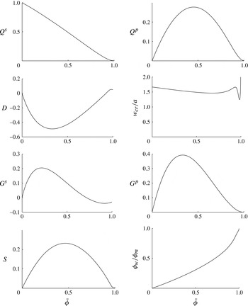
, which allows us to use spline interpolation and the asymptotic formulas (4.14)–(4.20) to restore the values of all functions in a fast and accurate manner. As an illustration, figure 5 plots the functions
 $Q^{s}$
,
 $Q^{p}$
,
 $D$
,
 $w_{cr}/a$
,
 $G^{s}$
,
 $G^{p}$
,
 $S$
and
 ${\it\phi}_{w}/{\it\phi}_{m}$
versus the normalized, average particle concentration
 $\bar{{\it\phi}}$
.
Variation of functions
 $Q^{s}$
,
 $Q^{p}$
,
 $D$
,
 $w_{cr}/a$
,
 $G^{s}$
,
 $G^{p}$
,
 $S$
and
 ${\it\phi}_{w}/{\it\phi}_{m}$
versus normalized average particle concentration
 $\bar{{\it\phi}}$
.

The critical width, appearing in (4.19), effectively precludes the proppant in areas where the fracture is narrow. But, as can be seen in figure 5, for most particle concentrations, this width is of the order of
 $1.5\times a$
, while it becomes unbounded for a very narrow region near
 $\bar{{\it\phi}}\approx 1$
. The particles, however, cannot physically be in a channel whose width is smaller than the particle diameter. Moreover, the bridging of the proppant may occur earlier when the fracture width is equal to several particle diameters. For this reason, there is a need to introduce a ‘blocking’ function, which would prevent the proppant entering the narrow regions. To this end, let us introduce
 $$\begin{eqnarray}B\left(\frac{w}{a}\right)=\frac{1}{2}H\left(\frac{w}{2a}-N\right)H\left(\frac{w_{B}-w}{2a}\right)\left[1+\cos \left({\rm\pi}\frac{w_{B}-w}{2a}\right)\right]+H\left(\frac{w-w_{B}}{2a}\right),\end{eqnarray}$$
where
 $N$
represents ‘several’ particle diameters (i.e. three),
 $H$
denotes the Heaviside step function, while
 $w_{B}=2a(N+1)$
, which provides a smooth vanishing of the function and helps the numerical implementation. To effectively prevent the proppant from moving into the narrow regions, the proppant flux in (4.6) needs to be multiplied by (4.21), in which case the proppant flux that is calculated according to
 $$\begin{eqnarray}\boldsymbol{q}_{B}^{p}=B\left(\frac{w}{a}\right)\boldsymbol{q}^{p}\end{eqnarray}$$
accounts for the proppant stalling in the narrow fracture regions.
4.1. Comments on the model
It is instructive to understand the physical meaning of all terms in the expressions for the fluxes in (4.5) and (4.6). The first term in the slurry flux is a Poiseuille flow-type term, where
 $Q^{s}(\bar{{\it\phi}})$
can be understood as the inverse of the effective viscosity of the mixture. As
 $\bar{{\it\phi}}$
approaches 1, the effective viscosity goes to infinity as
 $(1-\bar{{\it\phi}})^{-3/2}$
, as can be seen from (4.14). The second term in the slurry flow can be related to Darcy’s law. Indeed, according to Darcy’s law, the total flux through the channel is proportional to the pressure gradient, the permeability and the width of the channel. The permeability is proportional to the average squared pore size, which is, in turn, proportional to
 $a^{2}$
and some dimensionless function of
 $\bar{{\it\phi}}$
. Since
 $a/w\ll 1$
, for most particle concentrations, the flux is dominated by Poiseuille’s law. However, in the plugged regions (
 $\bar{{\it\phi}}\approx 1$
), one has
 $Q^{s}(\bar{{\it\phi}})\approx 0$
, while
 $D(\bar{{\it\phi}})>0$
, so that the flux is governed mainly by Darcy’s law. The remaining two terms represent the effect of gravity. In particular, they signify that, when the slurry is in a static position, i.e.
 $\boldsymbol{q}^{s}=0$
, the pressure is not equal to the hydrostatic pressure. Instead, there is a pressure gradient in addition to the hydrostatic pressure, which balances the shear stresses at the wall caused by the gravitational settling of particles. With regard to the flux of particles, the first term corresponds to the flux of particles ‘carried’ by the fluid, i.e. the advective term. The last two terms of the particle flux capture the effects associated with gravitational settling of the particles. One may also observe strange non-monotonic variation of
 $w_{cr}$
in figure 5. This is, unfortunately, one drawback of the constitutive model. This constitutive model is based on fitting. So while
 ${\it\mu}^{p}(\bar{{\it\phi}})$
may be accurate, the accuracy of its derivative may deteriorate significantly. Function
 $\mathscr{B}$
, (3.27), for instance, depends on the derivative of
 ${\it\mu}^{p}(\bar{{\it\phi}})$
, and
 $w_{cr}$
depends on
 $\mathscr{B}$
; see (4.12).
4.2. Simplified model
Despite the fact that (4.6) gives a complete answer for a broad range of parameters, the fact that the smallest fracture width where the proppant can be present is bounded by several particle diameters can be used to further simplify the result. The function
 $w_{cr}$
, shown in figure 5, is very steep, but monotone in the region
 $\bar{{\it\phi}}\approx 1$
, so can be inverted and be written in the form
 $\bar{{\it\phi}}_{w_{cr}}(w_{cr}/a)$
. Let us consider the case when
 $N=3$
in (4.21) and try to estimate the quantity
 $w^{2}-w_{cr}^{2}$
that appears in (4.6). In the worst case of
 $w=6a$
, this quantity vanishes for
 $1-\bar{{\it\phi}}_{w_{cr}}(6)=O(10^{-4})$
. Moreover,
 $1-\bar{{\it\phi}}_{w_{cr}}(2)=O(10^{-3})$
, in which case
 $w_{cr}^{2}/w^{2}<1/9$
for all possible values of
 $w$
(for which proppant can be inside the fracture). This shows that, if the term with
 $w_{cr}$
is neglected, a noticeable error may be introduced only for near-maximum concentrations
 $1-\bar{{\it\phi}}<O(10^{-3})$
. To see whether the variations of
 $\bar{{\it\phi}}$
in the region
 $1-\bar{{\it\phi}}<O(10^{-3})$
affect the slurry flow, one needs to compare the terms with
 $Q^{s}(\bar{{\it\phi}})$
and
 $D(\bar{{\it\phi}})$
in the slurry flux. To find the particle concentration, which characterizes the transition from Poiseuille’s to Darcy’s flow regime, one needs to express the relation
 $w^{2}Q^{s}(\bar{{\it\phi}})=a^{2}D(\bar{{\it\phi}})$
in the form
 $\bar{{\it\phi}}_{P-D}(w/a)$
. For the worst case
 $w=6a$
, it can be shown that
 $1-\bar{{\it\phi}}_{P-D}(6)=O(10^{-2})$
. As a result,
 $w_{cr}$
can be neglected, as
 $D({\it\phi})$
already dominates the flow for
 $1-\bar{{\it\phi}}<O(10^{-3})$
and its variations in this range are negligible (so that the error of 0.1 % in
 $\bar{{\it\phi}}$
does not lead to noticeable changes in the slurry flow). Moreover, the variations of
 $D$
are approximately equal to 5 % when
 $1-\bar{{\it\phi}}=O(10^{-2})$
, in which case
 $D(\bar{{\it\phi}})$
can be approximated by
 $\bar{{\it\phi}}D(1)$
(note that
 $D(\bar{{\it\phi}})$
should vanish for
 $\bar{{\it\phi}}=0$
). The estimation of the smallness of
 $w_{cr}^{2}/w^{2}$
is valid for the extreme case when
 $w=6a$
. In situations when
 $w/a>6$
, the asymptotic behaviour of
 $Q^{s}$
and
 $w_{cr}$
, (4.14) and (4.19), can be used to find that
 $1-\bar{{\it\phi}}_{P-D}(w/a)\propto (a/w)^{4/3}$
for the Poiseuille-to-Darcy transition, while
 $1-\bar{{\it\phi}}_{w_{cr}}(w/a)\propto (a/w)^{2}$
. This shows that the separation between the two characteristic values of
 $1-\bar{{\it\phi}}$
increases for bigger fracture widths (while they both decrease), which allows us to safely neglect
 $w_{cr}$
in (4.6) and use an approximation for
 $D(\bar{{\it\phi}})$
.
Since
 $a/w\ll 1$
, the gravity terms featured in (4.5) and (4.6) become important only for small values of the vertical pressure gradient, i.e.
 $\partial \widetilde{p^{\,f}}/\partial z=O(a^{2}/w^{2}({\it\rho}^{p}-{\it\rho}^{f})g)$
. This situation may occur when the hydraulic fracture is surrounded by stress barriers, since some hydraulic fracturing models even assume constant pressure in each vertical cross-section (see Adachi, Detournay & Peirce Reference Adachi, Detournay and Peirce2010). Owing to the presence of stress barriers, the pressure gradient in these fractures is predominantly horizontal, which could make the vertical component of the pressure gradient sufficiently small to cause
 $\partial \widetilde{p^{\,f}}/\partial z=O((a^{2}/w^{2})({\it\rho}^{p}-{\it\rho}^{f})g)$
. Note, however, that the absolute value of the pressure gradient may be big, and so
 $G_{{\it\rho}}$
, defined in (3.12), could be small. The fact that
 $(\partial \widetilde{p^{\,f}}/\partial z)/|\boldsymbol{{\rm\nabla}}\widetilde{p^{\,f}}|\ll 1$
allows us to neglect terms in (4.5) and (4.6) that are proportional to
 $(\partial \widetilde{p^{\,f}}/\partial z)/|\boldsymbol{{\rm\nabla}}\widetilde{p^{\,f}}|\ll 1$
, which reduces the complexity of the fluxes. Moreover, it is useful to introduce
 $$\begin{eqnarray}\widehat{p^{\,f}}=p^{\,f}-p_{h}^{\,f}=p^{\,f}+{\it\rho}^{f}gz+({\it\rho}^{p}-{\it\rho}^{f})g{\it\phi}_{m}\bar{{\it\phi}}z+({\it\rho}^{p}-{\it\rho}^{f})g\int _{0}^{z}\frac{a^{2}G^{s}(\bar{{\it\phi}})}{w^{2}Q^{s}(\bar{{\it\phi}})+a^{2}\bar{{\it\phi}}D(1)}\,\text{d}z^{\prime },\end{eqnarray}$$
which allows us to simplify (4.5) and (4.6) (also using the simplifications discussed in the previous paragraph) to
 $$\begin{eqnarray}\displaystyle & \displaystyle \boldsymbol{q}^{s}=-\frac{w^{3}}{12{\it\mu}^{f}}\hat{Q}^{s}\left(\bar{{\it\phi}},\frac{w}{a}\right)\boldsymbol{{\rm\nabla}}\widehat{p^{\,f}}, & \displaystyle\end{eqnarray}$$
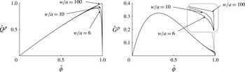
 $$\begin{eqnarray}\displaystyle & \displaystyle \boldsymbol{q}_{B}^{p}=B\left(\frac{w}{a}\right)\hat{Q}^{p}\left(\bar{{\it\phi}},\frac{w}{a}\right)\boldsymbol{q}^{s}-B\left(\frac{w}{a}\right)\frac{a^{2}w}{12{\it\mu}^{f}}({\it\rho}^{p}-{\it\rho}^{f})g\boldsymbol{e}_{z}{\hat{G}}^{p}\left(\bar{{\it\phi}},\frac{w}{a}\right), & \displaystyle\end{eqnarray}$$
 $$\begin{eqnarray}\displaystyle \displaystyle \hat{Q}^{s}\left(\bar{{\it\phi}},\frac{w}{a}\right) & = & \displaystyle \displaystyle Q^{s}(\bar{{\it\phi}})+\frac{a^{2}}{w^{2}}\bar{{\it\phi}}D(1),\end{eqnarray}$$
 $$\begin{eqnarray}\displaystyle \displaystyle \hat{Q}^{p}\left(\bar{{\it\phi}},\frac{w}{a}\right) & = & \displaystyle \displaystyle \frac{w^{2}Q^{p}(\bar{{\it\phi}})}{w^{2}Q^{s}(\bar{{\it\phi}})+a^{2}\bar{{\it\phi}}D(1)},\end{eqnarray}$$
 $$\begin{eqnarray}\displaystyle \displaystyle {\hat{G}}^{p}\left(\bar{{\it\phi}},\frac{w}{a}\right) & = & \displaystyle \displaystyle G^{p}(\bar{{\it\phi}})-\frac{w^{2}G^{s}(\bar{{\it\phi}})Q^{p}(\bar{{\it\phi}})}{w^{2}Q^{s}(\bar{{\it\phi}})+a^{2}\bar{{\it\phi}}D(1)}.\end{eqnarray}$$
 $p_{h}^{\,f}$
is the ‘true’ hydrostatic pressure in the sense that there is no motion of the slurry if
 $p^{\,f}=p_{h}^{\,f}$
. In terms of fluid-driven fracture problems, hydrostatic pressure is important for buoyancy-driven fractures (see e.g. Lister Reference Lister1990), while it is commonly neglected for other industrial hydraulic fracturing problems. In the simplified model (4.24)–(4.25), functions (4.26)–(4.28) determine the motion of the slurry and proppant. The function
 $\hat{Q}^{s}$
describes the slurry flow, and, in particular, accounts for the Poiseuille-to-Darcy transition of the flow. Clearly,
 $\hat{Q}^{p}$
describes convective proppant transport, while
 ${\hat{G}}^{p}$
captures gravitational settling. The fact that the model captures the Poiseuille-to-Darcy transition of the flow implies that both proppant transport and plugging (i.e. the formation of a zone with nearly maximum proppant concentration) are accounted for autonomously. As an illustration, figure 6 plots the variations of
 $\hat{Q}^{p}$
and
 ${\hat{G}}^{p}$
versus
 $\bar{{\it\phi}}$
for different values of
 $w/a=\{6,10,100\}$
. One can see that the parameter
 $w/a$
is important only in the regions with high particle concentration and leads to a smooth transition of functions
 $\hat{Q}^{p}$
and
 ${\hat{G}}^{p}$
to zero. It should be noted that there is almost no visual difference between
 $Q^{s}$
and
 $\hat{Q}^{s}$
. At the same time, qualitatively, there is a significant difference, since
 $Q^{s}$
goes to zero as
 $\bar{{\it\phi}}\rightarrow 1$
, while
 $\hat{Q}^{s}$
approaches a small constant. For the purpose of numerical calculations, the variation of functions
 $\hat{Q}^{p}$
and
 ${\hat{G}}^{p}$
versus
 $w/a$
can be approximated by taking either a limit
 $w/a\rightarrow \infty$
or
 $w/a=6$
, depending on the numerical scheme. As figure 6 shows, the error induced by such an approximation may slightly alter the dynamics of the plug (i.e. the region with a nearly maximum concentration), while the proppant transport at smaller concentrations will not be affected.
Variation of functions
 $\hat{Q}^{p}$
and
 ${\hat{G}}^{p}$
versus normalized average particle concentration
 $\bar{{\it\phi}}$
for different values of
 $w/a=\{6,10,100\}$
.

In the current simplified formulation, the functions
 $\hat{Q}^{s}$
,
 $\hat{Q}^{p}$
and
 ${\hat{G}}^{p}$
that enter (4.24)–(4.25) are based on this specific model for the slurry flow. In practical applications, however, all the assumptions of the model may not always be met and the model may deviate from the observations. For instance, the particles may be aspherical, or a mixture of particles with different sizes may be used. If a similar model cannot be derived, for example, owing to lack of a constitutive relation for the mixture, one possible solution is to keep all the terms in (4.24) and (4.25), but to modify the functions
 $\hat{Q}^{s}$
,
 $\hat{Q}^{p}$
and
 ${\hat{G}}^{p}$
to fit the data. For instance, one could measure the effective viscosity and permeability of the mixture and modify the functions accordingly. This formulation, therefore, represents a broad class of models, which could satisfy experimental observations, capture the Poiseuille-to-Darcy transition of the slurry flow, as well as particle transport and settling.
5. Summary
This paper studies the steady flow of a Newtonian fluid mixed with spherical particles under the influence of gravitational settling based on a continuum approach. The constitutive behaviour of the mixture is taken from an empirical model, where both the shear stress and particle pressure are expressed in terms of functions of the particle concentration. The solution obtained shows that the particles form a rigid cluster in the centre, and its size depends on the average concentration of the particles over the width. The velocity profile is shown to deviate from the classical parabolic shape for higher concentrations owing to a non-uniform distribution of particles. Also, the solution features a boundary layer, whose size is of the order of the particle radius. While the effect of the boundary layer is minimal for relatively small particle concentrations, it becomes crucial when the particle concentration is close to the maximum value. Unfortunately, the complicated nature of the solution obtained makes the result less valuable for hydraulic fracturing applications, as the implementation of such a complex model into a hydraulic fracturing simulator would be extremely cumbersome. For this reason, an approximate solution is introduced. To provide an estimate for the error that is introduced by the approximation, the ‘full’ solution is compared to the approximate solution for different regimes of the flow. It is shown that, even in the worst case when the pressure gradient is much weaker than the gravity force, the errors in the slurry flux and proppant flux do not exceed 30 %. For more realistic parameters, the error becomes even lower, of the order of 10 %.
The simplified approximate solution of the channel flow makes it possible to calculate the average fluxes for the slurry and the particles. These fluxes form the basis for the analysis of hydraulic fracturing by a slurry and the corresponding proppant transport problem. The simplified model (4.24)–(4.25) is now in a form that can be implemented in a hydraulic fracturing model that couples elasticity with slurry flow, and captures proppant transport, gravitational settling and plug formation.
Acknowledgements
The authors gratefully acknowledge the support of the British Columbia Oil and Gas Commission and the NSERC discovery grants programme. In addition, the authors would like to thank Professor E. Detournay (University of Minnesota) for stimulating the discussions at the inception of this project.