1. Introduction
Stratified and/or rotating fluids support waves which can transport and dissipate energy away from their sources. These waves are suspected to play an important role in atmospherical sciences, oceanography, and in the dynamics of stars and planets. In the atmosphere, they transport momentum from the convective regions to the high-altitude regions, where they break and create mean flow circulation (Fritts & Alexander Reference Fritts and Alexander2003). In the ocean, they are mostly generated by tide and winds and are expected to provide the missing contribution to the global energy budget of the ocean (Munk & Wunsch Reference Munk and Wunsch1998). In planets and stars, they are excited by gravitational effects (Le Bars, Cébron & Le Gal Reference Le Bars, Cébron and Le Gal2015) or convection (Rogers & Glatzmaier Reference Rogers and Glatzmaier2005) and could play a role in the generation of zonal flows (Tilgner Reference Tilgner2007) and in dissipative processes (Ogilvie & Lin Reference Ogilvie and Lin2004). In the present work, we are considering the simple configuration of a librating disk in a stratified and rotating fluid, for which an exact solution can be obtained to provide some general information on the structure of the wave field and its associated mean flow correction.
Libration is a harmonic forcing corresponding to an oscillation of the rotation rate. Such a forcing is present in most planets (Comstock & Bills Reference Comstock and Bills2003) due to their gravitational interaction with other surrounding massive objects. It corresponds to one of the possible mechanical forcings associated with gravitation, the others being tides and precession (see Le Bars et al. Reference Le Bars, Cébron and Le Gal2015). In the ocean, tide corresponds to the dominant harmonic forcing.
In a fluid, rotating with the rotation rate
 ${\it\Omega}^{\ast }$
around the axis
 $Oz$
and stably stratified with a constant buoyancy frequency
 $N^{\ast }$
along the same axis, these harmonic forcings excite waves when their frequency is in the inertia-gravity interval
 $I_{{\it\omega}}=\{\min (N^{\ast },2{\it\Omega}^{\ast })<{\it\omega}^{\ast }<\max (N^{\ast },2{\it\Omega}^{\ast })\}$
. These waves propagates along cones (in 3D) or planes (in 2D) with a fixed angle
 ${\it\alpha}$
with respect to the horizontal plane given by
 $\sin {\it\alpha}=\sqrt{({\it\omega}^{\ast 2}-4{\it\Omega}^{\ast 2})/(N^{\ast 2}-4{\it\Omega}^{\ast 2})}$
. The cone (or the plane) tangent to the oscillating object or to a local topographical feature corresponds to a singular surface across which the wave field changes its nature. The singularity of the wave field across these surfaces if smoothed by viscosity gives rise to thin internal shear layers which possess some generic features (Thomas & Stevenson Reference Thomas and Stevenson1972; Kerswell Reference Kerswell1995). These internal shear layers are visible when oscillating a small object as they form the familiar St Andrew’s cross pattern (Mowbray & Rarity Reference Mowbray and Rarity1967; Greenspan Reference Greenspan1968). They can also be observed tangent to the inner sphere when librating a rotating spherical shell (Koch et al.
Reference Koch, Harlander, Egbers and Hollerbach2013), or to a supercritical topography for tidal flow (Peacock, Echeverri & Balmforth Reference Peacock, Echeverri and Balmforth2008). These internal shear layers can be generated from singularities of the oscillating source too, such as from the corners of a cylinder (McEwan Reference McEwan1970) or from angular topography (St Laurent et al.
Reference St Laurent, Stringer, Garrett and Perrault-Joncas2003). They are the equivalent of the shear layer (Stewartson layer) limiting Taylor–Proudman columns in steady rotating flows for an oscillating flow in a stratified rotating fluid (Stewartson Reference Stewartson1957).
In a bounded geometry, harmonic forcings can also resonantly excite (normal) modes of the container (see, for instance, Aldridge & Toomre Reference Aldridge and Toomre1969; Rieutord Reference Rieutord1991). In a few specific geometries, such as the cylinder and the sphere, these modes have a regular inviscid structure which is now well known (Greenspan Reference Greenspan1968; Friedlander & Siegmann Reference Friedlander and Siegmann1982). However, in general, the inviscid modes are singular. Some of them are associated with an accumulation of waves on an attractor after multiple reflections on boundaries (see Rieutord & Valdettaro Reference Rieutord and Valdettaro1997; Rieutord, Georgeot & Valdettaro Reference Rieutord, Georgeot and Valdettaro2001). In a viscous framework, these attractors form a different type of internal layers from those described above. They have been observed in rectangular tanks (Maas et al. Reference Maas, Benielli, Sommeria and Lam1997) and in spherical shells (Tilgner Reference Tilgner1999; Koch et al. Reference Koch, Harlander, Egbers and Hollerbach2013). Because we are in an open domain, no mode resonances or attractors are our concern here.
In an open domain, most theoretical studies have focused on simple geometries (plane, disk, sphere, ellipsoid) for which the source term can be analytically described, and have often been concerned with the far field only. A comprehensive list of references, especially for stratified fluids, can be found in Voisin (Reference Voisin2003) and Voisin, Ermanyuk & Flór (Reference Voisin, Ermanyuk and Flór2011). The case of the disk has been considered in numerous works, for steady displacements in a rotating fluid (Stewartson Reference Stewartson1957; Moore & Saffman Reference Moore and Saffman1969; Vedensky & Ungarish Reference Vedensky and Ungarish1994; Tanzosh & Stone Reference Tanzosh and Stone1995), for oscillating displacements in a stratified fluid (Il’inyhk & Chashechkin Reference Il’inyhk and Chashechkin2004; Bardakov, Vasil’ev & Chashechkin Reference Bardakov, Vasil’ev and Chashechkin2007; Davis & Llewellyn Smith Reference Davis and Llewellyn Smith2010) or for more complicated surface fluctuations (Walton Reference Walton1975; Kerswell Reference Kerswell1995). The method of resolution is based on the use of the Hankel transform, which leads to a system of dual integral equations. These equations can then be converted into a system of algebraic equations using expansion in terms of Bessel functions (see, for instance, Davis & Llewellyn Smith Reference Davis and Llewellyn Smith2010). Here, we use the same method but the integral equations will turn out to have a simple explicit solution.
An important part of our work is concerned with the calculation of the mean flow generated by the nonlinear interaction of the harmonic response with itself. In a bounded non-stratified rotating fluid, these mean flow corrections are usually zonal flows (azimuthal flows), independent of the axial variable as prescribed by the Taylor–Proudman theorem. When there is no internal shear layer, they are dominantly generated by the nonlinear interactions occurring in the boundary layer (Busse Reference Busse1968). They can be calculated exactly for a cylinder (Wang Reference Wang1970; Sauret et al. Reference Sauret, Cébron, Le Bars and Le Dizès2012), a sphere and a spherical shell (Busse Reference Busse2010; Sauret & Le Dizès Reference Sauret and Le Dizès2013). In an infinite domain, we shall see that the mean flow corrections generated in the boundary are no longer purely azimuthal. Moreover, they are strongly modified by the stratification.
The presence of internal shear layers is expected to modify the mean flow corrections. In a spherical shell, both experiments (Morize et al. Reference Morize, Le Bars, Le Gal and Tilgner2010) and numerical simulations (Tilgner Reference Tilgner2007; Calkins et al. Reference Calkins, Noir, Eldredge and Aurnou2010) demonstrate that the zonal flow can exhibit very complicated structures which cannot be explained by classical boundary layer contributions only. Internal shear layers, especially close to the regions where they reflect on the boundary or on the axis, seem to strongly contribute to the zonal flow (Favier et al. Reference Favier, Barker, Baruteau and Ogilvie2014; Lin, Noir & Calkins Reference Lin, Noir and Calkins2014). We provide here both the scaling and the spatial structure of the zonal flow induced by the internal shear layers.
The paper is organized as follows. In § 2, the problem is presented and the basic equations are given. Section 3 is concerned with the calculation of the harmonic response. General expressions are first obtained, then reduced in each characteristic region (boundary layer, outer flow, internal shear layer, focus point on the axis) in the small-diffusion limit. In § 4, these expressions are used to calculate the mean flow correction. Stratified and non-stratified fluids are shown to give completely different mean flow corrections. A summary and a discussion of the main results are provided in §§ 5 and 6.
2. Framework
We consider a semi-infinite domain of incompressible fluid, delimited by a horizontal plane boundary
 $Oxy$
, rotating around the
 $Oz$
axis with an angular rotation
 ${\it\Omega}^{\ast }$
. The fluid is assumed to be stably stratified in the
 $Oz$
direction with a constant buoyancy frequency
 $N^{\ast }$
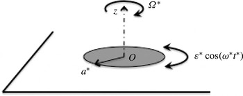
. Our goal is to describe the flow generated by librating a disk of radius
 $a^{\ast }$
centred on
 $O$
in the boundary (see the sketch in figure 1). The fluid satisfies no-slip boundary conditions such that in the rotating frame, the velocity field on the boundary can be written using cylindrical coordinates centred on the disk centre as
 $$\begin{eqnarray}\boldsymbol{V}^{\ast }=\left\{\begin{array}{@{}ll@{}}{\it\varepsilon}^{\ast }r^{\ast }\cos ({\it\omega}^{\ast }t^{\ast })\boldsymbol{e}_{{\it\theta}},\quad & r^{\ast }<a^{\ast },z^{\ast }=0,\\ 0,\quad & r^{\ast }>a^{\ast },z^{\ast }=0.\end{array}\right.\end{eqnarray}$$
The boundary is thermalized such that the buoyancy fluctuations
 $b$
(the temperature) are assumed to vanish on the boundary. This hypothesis can be relaxed when
 $Pr=\infty$
because the buoyancy then becomes a multiple of the vertical velocity. In that case, the buoyancy fluctuations also satisfy the boundary condition
 $\partial _{z}b=0$
relevant for configurations where the fluid is stratified in density. In the following, time and spatial variables are non-dimensionalized using
 $1/{\it\Omega}^{\ast }$
and
 $a^{\ast }$
. Non-dimensional quantities are indicated without asterisks.
Sketch of the flow geometry.

The problem is defined by five parameters: the librating amplitude
 ${\it\varepsilon}={\it\varepsilon}^{\ast }/{\it\Omega}^{\ast }$
, the librating frequency
 ${\it\omega}={\it\omega}^{\ast }/{\it\Omega}^{\ast }$
, the ratio
 $N=N^{\ast }/{\it\Omega}^{\ast }$
, the Ekman number
 $E={\it\nu}^{\ast }/({\it\Omega}a^{\ast 2})$
and the Prandtl number
 $Pr={\it\nu}^{\ast }/{\it\kappa}^{\ast }$
, where
 ${\it\nu}^{\ast }$
is the kinematic viscosity of the fluid and
 ${\it\kappa}^{\ast }$
the thermal diffusivity. We are interested in characterizing the periodic regime oscillating at the frequency
 ${\it\omega}$
when
 ${\it\varepsilon}$
and
 $E$
are both small. In particular, we do not consider the transient regime leading to this regime. We consider frequencies in the inertia-gravity frequency range
 $I_{{\it\omega}}=\{\min (2,N)<{\it\omega}<\max (2,N)\}$
, as well as frequencies outside this interval.
In the rotating frame, the velocity field
 $\boldsymbol{v}=(v_{r},v_{{\it\theta}},v_{z})$
and the pressure and buoyancy fluctuations
 $(P,B)$
satisfy the Boussinesq equations:
 $$\begin{eqnarray}\displaystyle & \displaystyle \frac{\text{D}\boldsymbol{v}}{\text{D}t}+2\boldsymbol{e}_{z}\wedge \boldsymbol{v}=-\boldsymbol{{\rm\nabla}}P-B\boldsymbol{e}_{z}+E{\rm\nabla}^{2}\boldsymbol{v}, & \displaystyle\end{eqnarray}$$
 $$\begin{eqnarray}\displaystyle & \boldsymbol{{\rm\nabla}}\boldsymbol{\cdot }\boldsymbol{v}=0, & \displaystyle\end{eqnarray}$$
 $$\begin{eqnarray}\displaystyle & \displaystyle \frac{\text{D}B}{\text{D}t}=N^{2}v_{z}+\displaystyle \frac{E}{Pr}{\rm\nabla}^{2}B. & \displaystyle\end{eqnarray}$$
We assume that the problem remains axisymmetrical. The linear response oscillating at the frequency
 ${\it\omega}$
can be written as
 $$\begin{eqnarray}\displaystyle (v_{r},v_{{\it\theta}},v_{z},P,B)={\it\varepsilon}(u,v,w,p,b)\text{e}^{-\text{i}{\it\omega}t}+\text{c.c.}, & & \displaystyle\end{eqnarray}$$
such that the pressure, buoyancy and velocity amplitudes satisfy the equations
 $$\begin{eqnarray}\displaystyle & \displaystyle -\text{i}{\it\omega}u-2v=-\displaystyle \frac{\partial p}{\partial r}+E\left({\it\Delta}-\frac{1}{r^{2}}\right)u, & \displaystyle\end{eqnarray}$$
 $$\begin{eqnarray}\displaystyle & \displaystyle -\text{i}{\it\omega}v+2u=+E\left({\it\Delta}-\frac{1}{r^{2}}\right)v, & \displaystyle\end{eqnarray}$$
 $$\begin{eqnarray}\displaystyle & \displaystyle -\text{i}{\it\omega}w=-\displaystyle \frac{\partial p}{\partial z}-b+E{\rm\Delta}w, & \displaystyle\end{eqnarray}$$
 $$\begin{eqnarray}\displaystyle & \displaystyle -\text{i}{\it\omega}b=N^{2}w+\displaystyle \frac{E}{Pr}{\rm\Delta}b, & \displaystyle\end{eqnarray}$$
 $$\begin{eqnarray}\displaystyle & \displaystyle \displaystyle \frac{\partial u}{\partial r}+\frac{u}{r}+\displaystyle \frac{\partial w}{\partial z}=0, & \displaystyle\end{eqnarray}$$
 ${\it\Delta}=\partial _{r}^{2}+(1/r)\partial _{r}+\partial _{z}^{2}$
, and the boundary conditions
 $$\begin{eqnarray}\displaystyle & u=w=b=0,v=r\quad \text{for}~r<1,z=0, & \displaystyle\end{eqnarray}$$
 $$\begin{eqnarray}\displaystyle & u=v=w=b=0\quad \text{for}~r>1,z=0, & \displaystyle\end{eqnarray}$$
 $$\begin{eqnarray}\displaystyle & u=v=w=b=0\quad \text{for}~r^{2}+z^{2}\rightarrow \infty . & \displaystyle\end{eqnarray}$$
We are also interested in the mean flow correction induced by the nonlinear interaction of the harmonic solution with itself. This correction can be written as
 ${\it\varepsilon}^{2}(u_{0},v_{0},w_{0},p_{0},b_{0})$
and satisfies
 $$\begin{eqnarray}\displaystyle & \displaystyle 2v_{0}-\displaystyle \frac{\partial p_{0}}{\partial r}+E\left({\it\Delta}-\frac{1}{r^{2}}\right)u_{0}=\left(u\displaystyle \frac{\partial u^{\ast }}{\partial r}+w\displaystyle \frac{\partial u^{\ast }}{\partial z}\right)-\frac{|v|^{2}}{r}+\text{c.c.}\equiv N_{u}, & \displaystyle\end{eqnarray}$$
 $$\begin{eqnarray}\displaystyle & \displaystyle -2u_{0}+E\left({\it\Delta}-\frac{1}{r^{2}}\right)v_{0}=\left(u\displaystyle \frac{\partial v^{\ast }}{\partial r}+w\displaystyle \frac{\partial v^{\ast }}{\partial z}\right)+\frac{uv^{\ast }}{r}+\text{c.c.}\equiv N_{v}, & \displaystyle\end{eqnarray}$$
 $$\begin{eqnarray}\displaystyle & \displaystyle -\displaystyle \frac{\partial p_{0}}{\partial z}-b_{0}+E{\rm\Delta}w_{0}=\left(u\displaystyle \frac{\partial w^{\ast }}{\partial r}+w\displaystyle \frac{\partial w^{\ast }}{\partial z}\right)+\text{c.c.}\equiv N_{w}, & \displaystyle\end{eqnarray}$$
 $$\begin{eqnarray}\displaystyle & \displaystyle N^{2}w_{0}-\displaystyle \frac{E}{Pr}{\rm\Delta}b_{0}=\left(u\displaystyle \frac{\partial b^{\ast }}{\partial r}+w\displaystyle \frac{\partial b^{\ast }}{\partial z}\right)+\text{c.c.}\equiv N_{b}, & \displaystyle\end{eqnarray}$$
 $$\begin{eqnarray}\displaystyle & \displaystyle \displaystyle \frac{\partial u_{0}}{\partial r}+\frac{u_{0}}{r}+\displaystyle \frac{\partial w_{0}}{\partial z}=0, & \displaystyle\end{eqnarray}$$
 $^{\ast }$
represents here the complex conjugate. The mean flow correction vanishes in the plane of the disk (
 $z=0$
) and at infinity (
 $r^{2}+z^{2}\rightarrow \infty$
). In the next two sections, we provide the spatial structures of the harmonic response and of the mean flow correction.
3. Harmonic response
In this section, we provide expressions for the linear harmonic response to the disk libration. As in Stewartson (Reference Stewartson1957), the harmonic response is sought using the Hankel transform as
 $$\begin{eqnarray}\displaystyle & \displaystyle u=\mathop{\sum }_{j=1}^{4}\int _{0}^{\infty }U_{j}(k)\text{J}_{1}(kr)\text{e}^{\text{i}{\it\mu}_{j}z}\,\text{d}k, & \displaystyle\end{eqnarray}$$
 $$\begin{eqnarray}\displaystyle & \displaystyle v=\mathop{\sum }_{j=1}^{4}\int _{0}^{\infty }V_{j}(k)\text{J}_{1}(kr)\text{e}^{\text{i}{\it\mu}_{j}z}\,\text{d}k, & \displaystyle\end{eqnarray}$$
 $$\begin{eqnarray}\displaystyle & \displaystyle w=\mathop{\sum }_{j=1}^{4}\int _{0}^{\infty }W_{j}(k)\text{J}_{0}(kr)\text{e}^{\text{i}{\it\mu}_{j}z}\,\text{d}k, & \displaystyle\end{eqnarray}$$
 $$\begin{eqnarray}\displaystyle & \displaystyle p=\mathop{\sum }_{j=1}^{4}\int _{0}^{\infty }P_{j}(k)\text{J}_{0}(kr)\text{e}^{\text{i}{\it\mu}_{j}z}\,\text{d}k, & \displaystyle\end{eqnarray}$$
 $$\begin{eqnarray}\displaystyle & \displaystyle b=\mathop{\sum }_{j=1}^{4}\int _{0}^{\infty }B_{j}(k)\text{J}_{0}(kr)\text{e}^{\text{i}{\it\mu}_{j}z}\,\text{d}k, & \displaystyle\end{eqnarray}$$
 ${\it\mu}={\it\mu}_{j}(k,{\it\omega}),j=1,2,3,4,$
are solutions of the dispersion relation deduced from (2.4a–e
),
 $$\begin{eqnarray}\displaystyle & & \displaystyle [-\text{i}{\it\omega}+E(k^{2}+{\it\mu}^{2})]^{2}[-\text{i}{\it\omega}+EPr^{-1}(k^{2}+{\it\mu}^{2})]({\it\mu}^{2}+k^{2})\nonumber\\ \displaystyle & & \displaystyle \quad +\,4{\it\mu}^{2}[-\text{i}{\it\omega}+EPr^{-1}(k^{2}+{\it\mu}^{2})]+N^{2}k^{2}[-\text{i}{\it\omega}+E(k^{2}+{\it\mu}^{2})]=0.\end{eqnarray}$$
Only the wavenumbers with a positive imaginary part (
 $\text{Im}\,({\it\mu}_{j})>0$
) have to be kept in order to satisfy the vanishing boundary conditions at infinity.
The coefficients are related to each other by the equations deduced from (2.4a–e ),
 $$\begin{eqnarray}\displaystyle & kU_{j}=-\text{i}{\it\mu}_{j}W_{j}, & \displaystyle\end{eqnarray}$$
 $$\begin{eqnarray}\displaystyle & 2U_{j}=-(-\text{i}{\it\omega}+E(k^{2}+{\it\mu}_{j}^{2}))V_{j}, & \displaystyle\end{eqnarray}$$
 $$\begin{eqnarray}\displaystyle & N^{2}W_{j}=(-\text{i}{\it\omega}+EPr^{-1}(k^{2}+{\it\mu}_{j}^{2}))B_{j}, & \displaystyle\end{eqnarray}$$
 $$\begin{eqnarray}\displaystyle & kP_{j}=-2V_{j}+(-\text{i}{\it\omega}+E(k^{2}+{\it\mu}_{j}^{2}))U_{j}. & \displaystyle\end{eqnarray}$$
 $z=0$
give
 $$\begin{eqnarray}\displaystyle & \displaystyle \mathop{\sum }_{j=1}^{4}\int _{0}^{\infty }U_{j}(k)\text{J}_{1}(kr)\,\text{d}k=0, & \displaystyle\end{eqnarray}$$
 $$\begin{eqnarray}\displaystyle & \displaystyle \mathop{\sum }_{j=1}^{4}\int _{0}^{\infty }V_{j}(k)\text{J}_{1}(kr)\,\text{d}k=r\text{H}(1-r), & \displaystyle\end{eqnarray}$$
 $$\begin{eqnarray}\displaystyle & \displaystyle \mathop{\sum }_{j=1}^{4}\int _{0}^{\infty }W_{j}(k)\text{J}_{0}(kr)\,\text{d}k=0, & \displaystyle\end{eqnarray}$$
 $$\begin{eqnarray}\displaystyle & \displaystyle \mathop{\sum }_{j=1}^{4}\int _{0}^{\infty }B_{j}(k)\text{J}_{0}(kr)\,\text{d}k=0, & \displaystyle\end{eqnarray}$$
 $\text{H}(z)$
is the Heaviside step function. Using (3.3a–d
), these equations form a system of integral equations for the coefficients
 $V_{j},j=1,2,3,4$
. Analogous equations were obtained by Tanzosh & Stone (Reference Tanzosh and Stone1995) and Davis & Llewellyn Smith (Reference Davis and Llewellyn Smith2010) for instance. Here, using the following property of the Bessel functions (Watson Reference Watson1952, P406):
 $$\begin{eqnarray}\displaystyle \int _{0}^{\infty }\text{J}_{2}(k)\text{J}_{1}(kr)\,\text{d}k=r\text{H}(1-r), & & \displaystyle\end{eqnarray}$$
the above system can be reduced to a simple algebraic system,
 $$\begin{eqnarray}\displaystyle \mathop{\sum }_{j=1}^{4}U_{j}(k)=\mathop{\sum }_{j=1}^{4}W_{j}(k)=\mathop{\sum }_{j=1}^{4}B_{j}(k)=0,\quad \mathop{\sum }_{j=1}^{4}V_{j}(k)=\text{J}_{2}(k). & & \displaystyle\end{eqnarray}$$
This system can be solved explicitly by expressing
 $U_{j}$
,
 $W_{j}$
and
 $B_{j}$
in terms of
 $V_{j}$
using (3.3a–d
).
We are interested in the weakly viscous configurations where
 $E$
is small and
 $Pr=O(1)$
. Simple expressions for the coefficients
 $U_{j}$
,
 $V_{j}$
,
 $W_{j}$
and
 $B_{j}$
are provided in appendix A in this limit. In this limit, the wavenumbers
 ${\it\mu}_{j},j=1,2,3,4$
, also simplify to
 $$\begin{eqnarray}{\it\mu}_{1}\sim {\it\epsilon}_{1}{\it\mu}_{1_{0}}k(1+\text{i}E{\it\alpha}k^{2}),\quad {\it\mu}_{2}\sim \frac{{\it\mu}_{2_{0}}}{\sqrt{E}},\quad {\it\mu}_{3}\sim \frac{{\it\mu}_{3_{0}}}{\sqrt{E}},\quad {\it\mu}_{4}\sim \frac{{\it\mu}_{4_{0}}}{\sqrt{E}},\end{eqnarray}$$
where
 $$\begin{eqnarray}\displaystyle {\it\mu}_{1_{0}}=\sqrt{\frac{N^{2}-{\it\omega}^{2}}{{\it\omega}^{2}-4}},\quad {\it\alpha}=\frac{(N^{2}-4)(N^{2}(4(Pr-1)+(Pr+1){\it\omega}^{2})-8Pr{\it\omega}^{2})}{2Pr{\it\omega}\left(4-{\it\omega}^{2}\right)^{2}({\it\omega}^{2}-N^{2})},\end{eqnarray}$$
 $$\begin{eqnarray}\displaystyle {\it\mu}_{2_{0}}=\frac{(1+\text{i})}{\sqrt{2}}\sqrt{{\it\omega}-2},\quad {\it\mu}_{3_{0}}=\frac{(1+\text{i})}{\sqrt{2}}\sqrt{{\it\omega}+2},\quad {\it\mu}_{4_{0}}=\frac{(1+\text{i})}{\sqrt{2}}\sqrt{{\it\omega}Pr},\end{eqnarray}$$
and where the square root has been defined such that the square root of a negative number is a positive imaginary number. The parameter
 ${\it\epsilon}_{1}=\pm 1$
in (3.7) is chosen such that
 $\text{Im}({\it\mu}_{1})>0$
. We then obtain
 ${\it\epsilon}_{1}=\text{sgn}(2-N)$
when
 ${\it\omega}\in I_{{\it\omega}}$
and
 ${\it\epsilon}_{1}=1$
when
 ${\it\omega}\notin I_{{\it\omega}}$
.
In the above expressions, we have implicitly assumed that
 $k$
,
 $Pr$
,
 $N$
and
 ${\it\omega}$
are of order 1 and that
 ${\it\omega}$
is distinct from 2 and
 $N$
. Below, we also consider the cases
 $N=0$
and
 $Pr=\infty$
. The first limit is regular and we can use the same expressions when
 $N=0$
. In this limit, the buoyancy fluctuations are found to vanish everywhere. When
 $Pr=\infty$
,
 $\text{Im}({\it\mu}_{4_{0}})$
goes to infinity, which means that the part of the solution associated with
 ${\it\mu}_{4}$
disappears. In that limit, the solution is then only a sum on the first three waves. All of the expressions concerning these waves are regular in the limit
 $Pr\rightarrow \infty$
.
The first wavenumber
 ${\it\mu}_{1}$
corresponds to the so-called inertia-gravity wave, the second and third wavenumbers
 ${\it\mu}_{2}$
and
 ${\it\mu}_{3}$
are viscous wavenumbers, while the fourth wavenumber
 ${\it\mu}_{4}$
is a thermal wavenumber. It should be noted that the viscous and thermal wavenumbers are both large when
 $E$
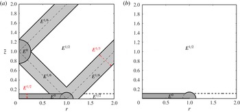
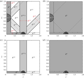
is small. The contributions from these waves to the harmonic response are then expected to be exponentially small far away from the boundary. More precisely, theses waves would be present in the boundary layer only. In the following subsections, we provide simple expressions for the harmonic response in the different characteristic regions of the fluid. The scalings of the amplitude of the solution in these different regions are summarized in figure 12 of § 5.
3.1. Boundary layer on the disk
Close to the boundary, all of the waves are present in the solution. Using the relation
 $$\begin{eqnarray}\displaystyle \int _{0}^{\infty }k\text{J}_{2}(k)\text{J}_{0}(kr)\,\text{d}k=2\text{H}(1-r)-{\it\delta}(r-1), & & \displaystyle\end{eqnarray}$$
and the expressions given in appendix A for the coefficients, we obtain the following expression for the harmonic response in the boundary layer on the disk (
 $r<1,z=O(\sqrt{E})$
):
 $$\begin{eqnarray}\displaystyle (u,v,w,b)\sim (\bar{u},\bar{v},\sqrt{E}\,\bar{w},\sqrt{E}\,\bar{b}), & & \displaystyle\end{eqnarray}$$
with
 $$\begin{eqnarray}\displaystyle & \displaystyle \bar{u}(r,\bar{z})=-\frac{\text{i}r}{2}(\text{e}^{\text{i}{\it\mu}_{3_{0}}\bar{z}}-\text{e}^{\text{i}{\it\mu}_{2_{0}}\bar{z}}), & \displaystyle\end{eqnarray}$$
 $$\begin{eqnarray}\displaystyle & \displaystyle \bar{v}(r,\bar{z})=\frac{r}{2}(\text{e}^{\text{i}{\it\mu}_{3_{0}}\bar{z}}+\text{e}^{\text{i}{\it\mu}_{2_{0}}\bar{z}}), & \displaystyle\end{eqnarray}$$
 $$\begin{eqnarray}\displaystyle & \displaystyle \bar{w}(\bar{z})=\text{e}^{-\text{i}{\rm\pi}/4}\left(\frac{1-\text{e}^{\text{i}{\it\mu}_{2_{0}}\bar{z}}}{\sqrt{{\it\omega}-2}}+\frac{\text{e}^{\text{i}{\it\mu}_{3_{0}}\bar{z}}-1}{\sqrt{{\it\omega}+2}}\right), & \displaystyle\end{eqnarray}$$
 $$\begin{eqnarray}\displaystyle & \displaystyle \bar{b}(\bar{z})=\text{e}^{\text{i}{\rm\pi}/4}\left(b_{00}-\displaystyle \frac{N^{2}Pr\text{e}^{\text{i}{\it\mu}_{2_{0}}\bar{z}}}{\sqrt{{\it\omega}-2}({\it\omega}(Pr-1)+2)}+\displaystyle \frac{N^{2}Pr\text{e}^{\text{i}{\it\mu}_{3_{0}}\bar{z}}}{\sqrt{{\it\omega}+2}({\it\omega}(Pr-1)-2)}+b_{04}\text{e}^{\text{i}{\it\mu}_{4_{0}}\bar{z}}\right), & \displaystyle \nonumber\\ \displaystyle & & \displaystyle\end{eqnarray}$$
 $\bar{z}$
is the boundary layer variable
 $\bar{z}=z/\sqrt{E}$
and
 $$\begin{eqnarray}\displaystyle & \displaystyle b_{00}=\frac{N^{2}}{{\it\omega}}\left(\frac{1}{\sqrt{{\it\omega}-2}}-\frac{1}{\sqrt{{\it\omega}+2}}\right), & \displaystyle\end{eqnarray}$$
 $$\begin{eqnarray}\displaystyle & \displaystyle b_{04}=\frac{N^{2}}{{\it\omega}}\left(\frac{\sqrt{{\it\omega}-2}}{{\it\omega}(Pr-1)+2}-\frac{\sqrt{{\it\omega}+2}}{{\it\omega}(Pr-1)-2}\right). & \displaystyle\end{eqnarray}$$
 ${\it\omega}=\pm 2/(Pr-1)$
. For these values of the frequency, the thermal wavenumber equals one of the viscous wavenumbers and the solution is not a sum of exponentials anymore. It should be noted also that the velocity field does not depend on stratification in the boundary layer, a property that has been known for a long time (Barcilon & Pedlosky Reference Barcilon and Pedlosky1967).
In the boundary layer ouside the disk (
 $r>1,z=O(\sqrt{E})$
), the horizontal velocity components obtained from the leading-order expression of the coefficients vanish. One could easily show that they are
 $O(\sqrt{E})$
smaller than on the disk (
 $r<1,z=O(\sqrt{E})$
).
3.2. Outer region (away from the boundary)
In the outer region, far from the boundary, the solution is dominated by the wave associated with the inertia-gravity wavenumber
 ${\it\mu}_{1}$
, the other waves being exponentially small. When
 ${\it\omega}\notin I_{{\it\omega}}$
,
 ${\it\mu}_{1}$
is purely imaginary at leading order and can be written as
 ${\it\mu}_{1}\sim \text{i}|{\it\mu}_{1_{0}}|k$
. Using the expressions of appendix A for the coefficients
 $U_{1}$
,
 $V_{1}$
,
 $W_{1}$
and
 $B_{1}$
, we obtain, when
 ${\it\omega}\notin I_{{\it\omega}}$
,
 $$\begin{eqnarray}\displaystyle & \displaystyle u\sim \text{i}\sqrt{E}\,\frac{{\it\omega}v_{1}}{2}K^{(1)}(r,\tilde{z}), & \displaystyle\end{eqnarray}$$
 $$\begin{eqnarray}\displaystyle & \displaystyle v\sim \sqrt{E}\,v_{1}K^{(1)}(r,\tilde{z}), & \displaystyle\end{eqnarray}$$
 $$\begin{eqnarray}\displaystyle & \displaystyle w\sim \text{i}\sqrt{E}\,\frac{{\it\omega}v_{1}}{2|{\it\mu}_{1_{0}}|}K^{(0)}(r,\tilde{z}), & \displaystyle\end{eqnarray}$$
 $$\begin{eqnarray}\displaystyle & \displaystyle b\sim -\sqrt{E}\,\frac{N^{2}v_{1}}{2|{\it\mu}_{1_{0}}|}K^{(0)}(r,\tilde{z}), & \displaystyle\end{eqnarray}$$
 $$\begin{eqnarray}\displaystyle K^{(n)}(r,\tilde{z})=\int _{0}^{\infty }k\text{J}_{2}(k)\text{J}_{n}(kr)\text{e}^{-k\tilde{z}}\,\text{d}k & & \displaystyle\end{eqnarray}$$
and
 $$\begin{eqnarray}\displaystyle \tilde{z}=|{\it\mu}_{1_{0}}|z. & & \displaystyle\end{eqnarray}$$
The coefficients
 $v_{1}$
and
 ${\it\mu}_{1_{0}}$
have been defined in (A 2a
) and (3.8a
) respectively. The spatial structure of the functions
 $K^{(0)}$
and
 $K^{(1)}$
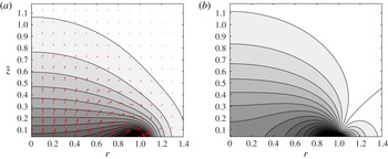
is shown in figure 2, where we have plotted the contours of the norm and the vector field of the poloidal field
 $(U,W)=(K^{(1)},K^{(0)})$
, and the contours of the angular velocity
 $V/r=K^{(1)}/r$
.
Flow structure in the bulk when
 ${\it\omega}\notin I_{{\it\omega}}$
. (a) Contours of the norm and vector field of the poloidal velocity field
 $(u,w)=(K^{(1)},K^{(0)})$
. (b) Contours of the angular velocity field
 ${\it\Omega}=K^{(1)}/r$
.

When
 ${\it\omega}\in I_{{\it\omega}}$
, we obtain similar expressions:
 $$\begin{eqnarray}\displaystyle & \displaystyle u\sim \text{i}\sqrt{E}\frac{{\it\omega}v_{1}}{2}F_{{\it\epsilon}_{1}}^{(1)}(r,\tilde{z}), & \displaystyle\end{eqnarray}$$
 $$\begin{eqnarray}\displaystyle & \displaystyle v\sim \sqrt{E}v_{1}F_{{\it\epsilon}_{1}}^{(1)}(r,\tilde{z}), & \displaystyle\end{eqnarray}$$
 $$\begin{eqnarray}\displaystyle & \displaystyle w\sim -{\it\epsilon}_{1}\sqrt{E}\frac{{\it\omega}v_{1}}{2{\it\mu}_{1_{0}}}F_{{\it\epsilon}_{1}}^{(0)}(r,\tilde{z}), & \displaystyle\end{eqnarray}$$
 $$\begin{eqnarray}\displaystyle & \displaystyle b\sim -\text{i}{\it\epsilon}_{1}\sqrt{E}\frac{N^{2}v_{1}}{2{\it\mu}_{1_{0}}}F_{{\it\epsilon}_{1}}^{(0)}(r,\tilde{z}), & \displaystyle\end{eqnarray}$$
 $$\begin{eqnarray}\displaystyle F_{{\it\epsilon}_{1}}^{(n)}(r,\tilde{z})=\int _{0}^{\infty }k\text{J}_{2}(k)\text{J}_{n}(kr)\text{e}^{\text{i}{\it\epsilon}_{1}k\tilde{z}}\,\text{d}k. & & \displaystyle\end{eqnarray}$$
The phase of the solution mainly depends on the phase of
 $v_{1}$
, which varies with
 ${\it\omega}$
according to (A 3). It should be noted, however, that
 $u$
and
 $v$
on the one hand, and
 $w$
and
 $b$
on the other hand, are always in phase quadrature whatever
 ${\it\omega}$
. The amplitudes
 $v$
and
 $w$
are also in phase quadrature when
 ${\it\omega}\notin I_{{\it\omega}}$
.
It should be noted that the harmonic response in the outer region is at leading order independent of
 $Pr$
. The dependence with respect to
 $N$
and
 ${\it\omega}$
is also particularly simple as these parameters only appear through rescaling factors in the velocity components and in the axial variable.
Whereas the harmonic response is regular in the bulk when
 ${\it\omega}\notin I_{{\it\omega}}$
, the harmonic response for
 ${\it\omega}\in I_{{\it\omega}}$
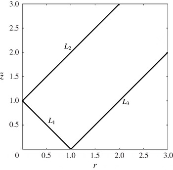
exhibits singularities on the characteristic lines
 $L_{j}$
,
 $j=1,2,3$
, shown in figure 3. These lines correspond to the line of propagation of the singularity at the disk edge, already mentioned in the introduction. They are defined by
 $$\begin{eqnarray}\displaystyle & L_{1}=\{(r,\tilde{z}),r=1-\tilde{z},0<\tilde{z}<1\}, & \displaystyle\end{eqnarray}$$
 $$\begin{eqnarray}\displaystyle & L_{2}=\{(r,\tilde{z}),r=-1+\tilde{z},\tilde{z}>1\}, & \displaystyle\end{eqnarray}$$
 $$\begin{eqnarray}\displaystyle & L_{3}=\{(r,\tilde{z}),r=1+\tilde{z},\tilde{z}>0\}. & \displaystyle\end{eqnarray}$$
 ${\it\mu}_{1}$
(see expression (3.7)) and use the following expression for
 $F_{{\it\epsilon}_{1}}^{(n)}$
in (3.16):
 $$\begin{eqnarray}\displaystyle F_{{\it\epsilon}_{1}}^{(n)}(r,\tilde{z},\tilde{E})=\int _{0}^{\infty }k\text{J}_{2}(k)\text{J}_{n}(kr)\text{e}^{\text{i}{\it\epsilon}_{1}k\tilde{z}}\text{e}^{-\tilde{E}k^{3}\tilde{z}}\,\text{d}k, & & \displaystyle\end{eqnarray}$$
with
 $$\begin{eqnarray}\displaystyle \tilde{E}=|{\it\alpha}|E, & & \displaystyle\end{eqnarray}$$
where
 ${\it\alpha}$
has been defined in (3.8a
). In the next two sections, we show that close to the lines
 $L_{j}$
, and at their crossing point on the axis, the solution takes a simple form.
Definitions of the lines
 $L_{j}$
,
 $j=1,2,3$
, in the
 $(r,\tilde{z})$
plane.

It should be noted that because
 $\text{J}_{2}(k)=2\text{J}_{1}(k)/k-\text{J}_{0}(k)$
, the harmonic response in the outer region is exactly the sum of two contributions:
-
(i) a disk contribution corresponding to a uniform oscillating vertical flow on the disk of amplitude
 $\tilde{w}_{d}=-{\it\epsilon}_{1}{\it\omega}v_{1}/({\it\mu}_{1_{0}})\sqrt{E}$
whose solution is (3.21)
$$\begin{eqnarray}\displaystyle w_{d}=\tilde{w}_{d}\int _{0}^{\infty }\text{J}_{1}(k)\text{J}_{0}(kr)\text{e}^{\text{i}{\it\epsilon}_{1}k\tilde{z}}\text{e}^{-\tilde{E}k^{3}\tilde{z}}\,\text{d}k; & & \displaystyle\end{eqnarray}$$
-
(ii) a ring contribution corresponding to a Dirac oscillating vertical flow at the disk edge of amplitude
$\tilde{w}_{r}={\it\epsilon}_{1}{\it\omega}v_{1}/(2{\it\mu}_{1_{0}})\sqrt{E}$
whose solution is (3.22)
$$\begin{eqnarray}\displaystyle w_{r}=\tilde{w}_{r}\int _{0}^{\infty }k\text{J}_{0}(k)\text{J}_{0}(kr)\text{e}^{\text{i}{\it\epsilon}_{1}k\tilde{z}}\text{e}^{-\tilde{E}k^{3}\tilde{z}}\,\text{d}k. & & \displaystyle\end{eqnarray}$$


These two contributions have been analysed separately by Tilgner (Reference Tilgner2000). We discuss this point again in § 6.
3.3. Close to the singularity lines
Due to the presence of singularities on the lines
 $L_{j}$
,
 $j=1,2,3$
, we expect the main contribution to the viscous integral (3.19) to come, close to these lines, from large values of
 $k$
. This allows us to use the asymptotic expansion of the Bessel functions
 $\text{J}_{m}(y)$
as
 $y\rightarrow \infty$
:
 $$\begin{eqnarray}\displaystyle \text{J}_{m}(y)\sim \sqrt{\frac{2}{{\rm\pi}y}}\cos \left(y-\frac{{\rm\pi}}{4}-\frac{m{\rm\pi}}{2}\right). & & \displaystyle\end{eqnarray}$$
The function
 $F_{{\it\epsilon}_{1}}^{(n)}$
given in (3.19) reduces near these lines to an expression of the form
 $$\begin{eqnarray}\displaystyle F_{{\it\epsilon}_{1}}^{(n)}(r,\tilde{z},\tilde{E})\sim \frac{\text{e}^{\text{i}h_{j}^{(n)}}}{\tilde{E}^{1/3}\sqrt{1+{\it\mu}_{1_{0}}^{2}}\sqrt{r}}L_{{\it\epsilon}_{1}}({\it\eta}_{\bot },{\it\zeta}), & & \displaystyle\end{eqnarray}$$
where the transverse variable
 ${\it\eta}_{j\bot }$
and the phase factor
 $h_{j}^{(n)}$
are defined for each line
 $L_{j},j=1,2,3$
, by
 $$\begin{eqnarray}{\it\eta}_{1\bot }=\displaystyle \frac{{\it\mu}_{1_{0}}z+(r-1)}{\tilde{E}^{1/3}\sqrt{1+{\it\mu}_{1_{0}}^{2}}},\quad h_{1}^{(1)}={\it\epsilon}_{1}{\rm\pi}/2,\quad h_{1}^{(0)}={\rm\pi},\end{eqnarray}$$
 $$\begin{eqnarray}{\it\eta}_{2\bot }=\displaystyle \frac{{\it\mu}_{1_{0}}z-(r+1)}{\tilde{E}^{1/3}\sqrt{1+{\it\mu}_{1_{0}}^{2}}},\quad h_{2}^{(1)}=1,\quad h_{2}^{(0)}=-{\it\epsilon}_{1}{\rm\pi}/2,\end{eqnarray}$$
 $$\begin{eqnarray}{\it\eta}_{3\bot }=\displaystyle \frac{{\it\mu}_{1_{0}}z-(r-1)}{\tilde{E}^{1/3}\sqrt{1+{\it\mu}_{1_{0}}^{2}}},\quad h_{3}^{(1)}=-{\it\epsilon}_{1}{\rm\pi}/2,\quad h_{3}^{(0)}={\rm\pi},\end{eqnarray}$$
and
 $$\begin{eqnarray}\displaystyle {\it\zeta}=\frac{{\it\mu}_{1_{0}}}{(1+{\it\mu}_{1_{0}}^{2})^{3/2}}z. & & \displaystyle\end{eqnarray}$$
The function
 $L_{{\it\epsilon}_{1}}$
is defined by
 $$\begin{eqnarray}\displaystyle L_{{\it\epsilon}_{1}}({\it\eta}_{\bot },{\it\zeta})=\frac{1}{2{\rm\pi}}\int _{0}^{\infty }\text{e}^{\text{i}{\it\epsilon}_{1}k{\it\eta}_{\bot }}\text{e}^{-k^{3}{\it\zeta}}\,\text{d}k=\frac{1}{2(3{\it\zeta})^{1/3}}\text{Hi}\left(\text{i}{\it\epsilon}_{1}\frac{{\it\eta}_{\bot }}{(3{\it\zeta})^{1/3}}\right), & & \displaystyle\end{eqnarray}$$
where the function
 $\text{Hi}$
is the Scorer’s function (Abramowitz & Stegun Reference Abramowitz and Stegun1965, page 448), defined by
 $$\begin{eqnarray}\displaystyle \text{Hi}(z)=\frac{1}{{\rm\pi}}\int _{0}^{\infty }\text{e}^{zk-k^{3}/3}\,\text{d}k. & & \displaystyle\end{eqnarray}$$
It satisfies
 $\text{Hi}^{\prime \prime }-z\text{Hi}(z)={\rm\pi}^{-1}$
and is such that
 $\text{Hi}(\text{i}z)\sim \text{i}/({\rm\pi}z)$
when
 $z\rightarrow \pm \infty$
. Additional properties can be found in Drazin & Reid (Reference Drazin and Reid1981), page 470, where it corresponds to the generalized Airy function
 $B_{1}(z,0)$
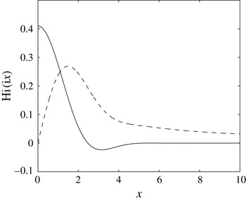
, or in appendix B of Voisin (Reference Voisin2003). It was first introduced for the description of internal shear layers by Moore & Saffman (Reference Moore and Saffman1969) and Thomas & Stevenson (Reference Thomas and Stevenson1972). The real and imaginary parts of the function
 $\text{Hi}(\text{i}z)$
that describes the structure of the harmonic response near the lines
 $L_{j}$
are plotted in figure 4.
The function
 $\text{Hi}(\text{i}x)$
versus
 $x$
. The solid line is the real part and the dashed line is the imaginary part.

The above expressions can be used to show that around each line
 $L_{j}$
, the velocity field is mainly composed of the azimuthal component and a component
 $v_{\Vert }$
aligned along with
 $L_{j}$
. For the line
 $L_{1}$
,
 $v_{\bot }$
and
 $v_{\Vert }$
are defined by
 $$\begin{eqnarray}\displaystyle v_{\bot }=\frac{u+{\it\mu}_{1_{0}}w}{\sqrt{1+{\it\mu}_{1_{0}}^{2}}},\quad v_{\Vert }=\frac{w-{\it\mu}_{1_{0}}u}{\sqrt{1+{\it\mu}_{1_{0}}^{2}}}, & & \displaystyle\end{eqnarray}$$
while for
 $L_{2}$
and
 $L_{3}$
, they are given by
 $$\begin{eqnarray}\displaystyle v_{\bot }=\frac{{\it\mu}_{1_{0}}w-u}{\sqrt{1+{\it\mu}_{1_{0}}^{2}}},\quad v_{\Vert }=\frac{w+{\it\mu}_{1_{0}}u}{\sqrt{1+{\it\mu}_{1_{0}}^{2}}}. & & \displaystyle\end{eqnarray}$$
We obtain
 $v\sim E^{1/6}\tilde{v}$
,
 $b\sim E^{1/6}\tilde{b}$
and
 $v_{\Vert }\sim E^{1/6}\tilde{v}_{\Vert }$
, where
 $$\begin{eqnarray}\displaystyle & \displaystyle \tilde{v}\sim \tilde{V}\text{e}^{\text{i}h_{j}^{(1)}}\frac{L_{{\it\epsilon}_{1}}({\it\eta}_{j\bot },{\it\zeta})}{\sqrt{r}}, & \displaystyle\end{eqnarray}$$
 $$\begin{eqnarray}\displaystyle & \displaystyle \tilde{b}\sim \tilde{B}\text{e}^{\text{i}k_{j}}\frac{L_{{\it\epsilon}_{1}}({\it\eta}_{j\bot },{\it\zeta})}{\sqrt{r}}, & \displaystyle\end{eqnarray}$$
 $$\begin{eqnarray}\displaystyle & \displaystyle \tilde{v}_{\Vert }\sim \tilde{V}_{\Vert }\text{e}^{\text{i}l_{j}}\frac{L_{{\it\epsilon}_{1}}({\it\eta}_{j\bot },{\it\zeta})}{\sqrt{r}}, & \displaystyle\end{eqnarray}$$
 $$\begin{eqnarray}\displaystyle \tilde{V}=\frac{v_{1}}{2{\it\alpha}^{1/3}\sqrt{1+{\it\mu}_{1_{0}}^{2}}},\quad \tilde{B}=\frac{N^{2}\tilde{V}}{2{\it\mu}_{1_{0}}},\quad \tilde{V}_{\Vert }=\frac{{\it\omega}\sqrt{1+{\it\mu}_{1_{0}}^{2}}}{2{\it\mu}_{1_{0}}}\tilde{V}, & & \displaystyle\end{eqnarray}$$
where
 $v_{1}$
,
 ${\it\mu}_{1_{0}}$
and
 ${\it\alpha}$
have been defined in (A 2a
) and (3.8a
). The phase of the component
 $v_{\Vert }$
is in quadrature with
 $v$
and
 $b$
and satisfies
 $l_{1}=h_{1}^{(1)}+{\rm\pi}/2=k_{1}-{\rm\pi}/2$
and
 $l_{j}=h_{j}^{(1)}-{\rm\pi}/2=k_{j}-{\rm\pi}/2$
for
 $j=2,3$
.
The velocity component
 $v_{\bot }$
is
 $O(E^{1/3})$
smaller than
 $v$
and
 $v_{\Vert }$
. Writing
 $v_{\bot }=E^{1/2}\tilde{v}_{\bot }$
, it can be obtained from the incompressibility condition
 $$\begin{eqnarray}\displaystyle \displaystyle \frac{\partial \tilde{v}_{\bot }}{\partial {\it\eta}_{\bot }}=-\displaystyle \frac{\partial \tilde{v}_{\Vert }}{\partial {\it\eta}_{\Vert }}, & & \displaystyle\end{eqnarray}$$
using
 $$\begin{eqnarray}\displaystyle \displaystyle \frac{\partial }{\partial {\it\eta}_{\Vert }}=\left\{\begin{array}{@{}l@{}}\displaystyle \displaystyle \frac{{\it\mu}_{1_{0}}}{\sqrt{1+{\it\mu}_{1_{0}}^{2}}}\left(\frac{1}{(1+{\it\mu}_{1_{0}}^{2})^{3/2}}\displaystyle \frac{\partial }{\partial {\it\zeta}}-\displaystyle \frac{\partial }{\partial r}\right)\quad \text{for}~L_{1},\\ \displaystyle \displaystyle \frac{{\it\mu}_{1_{0}}}{\sqrt{1+{\it\mu}_{1_{0}}^{2}}}\left(\frac{1}{(1+{\it\mu}_{1_{0}}^{2})^{3/2}}\displaystyle \frac{\partial }{\partial {\it\zeta}}+\displaystyle \frac{\partial }{\partial r}\right)\quad \text{for }L_{2}\text{ and }L_{3}.\end{array}\right. & & \displaystyle\end{eqnarray}$$
To close this section, it is worth noting that the flow structure obtained close to the singularity lines is associated with the ring source at the disk edge only. The other source (uniform flow on the disk) gives a wave field that is
 $O(E^{1/3})$
smaller close to the singularity lines. We discuss the consequences of this result in § 6.
3.4. Close to the focus point
$(r,\tilde{z})=(0,1)$

When
 $r$
goes to zero, the lines
 $L_{1}$
and
 $L_{2}$
collide at
 $\tilde{z}=1$
. This particular region close to the axis also corresponds to the peaks of the cones formed by the lines
 $L_{1}$
and
 $L_{2}$
. As the rays are focused to this particular point, we expect larger amplitudes, as also predicted by (3.31a–c
) which diverge as
 $r\rightarrow 0$
. A local solution can be obtained from (3.16) and (3.19) by introducing the local variables
 $R=r\tilde{E}^{-1/3}$
and
 $Z=(\tilde{z}-1)\tilde{E}^{-1/3}$
, and using the expansion (3.23) of one of the Bessel functions only. We first obtain
 $$\begin{eqnarray}\displaystyle & F_{{\it\epsilon}_{1}}^{(1)}\sim \tilde{E}^{-1/2}\text{e}^{\text{i}{\it\epsilon}_{1}5{\rm\pi}/4}\text{H}_{{\it\epsilon}_{1}}^{(1,1)}(R,Z), & \displaystyle\end{eqnarray}$$
 $$\begin{eqnarray}\displaystyle & F_{{\it\epsilon}_{1}}^{(0)}\sim \tilde{E}^{-1/2}\text{e}^{\text{i}{\it\epsilon}_{1}5{\rm\pi}/4}\text{H}_{{\it\epsilon}_{1}}^{(1,0)}(R,Z), & \displaystyle\end{eqnarray}$$
 $$\begin{eqnarray}\displaystyle \text{H}_{{\it\epsilon}_{1}}^{(m,n)}(R,Z)=\frac{1}{\sqrt{2{\rm\pi}}}\int _{0}^{+\infty }k^{m-1/2}\text{J}_{n}(kR)\text{e}^{\text{i}{\it\epsilon}_{1}kZ-k^{3}}\,\text{d}k, & & \displaystyle\end{eqnarray}$$
from which we obtain
 $$\begin{eqnarray}\displaystyle \left(\begin{array}{@{}c@{}}u\\ v\\ w\\ b\end{array}\right)=\frac{v_{1}}{|{\it\alpha}|^{1/2}}\left(\begin{array}{@{}ccc@{}}{\it\omega}/2 & \text{e}^{\text{i}{\it\epsilon}_{1}{\rm\pi}/4+\text{i}{\rm\pi}/2} & \text{H}_{{\it\epsilon}_{1}}^{(1,1)}(R,Z)\\ & \text{e}^{\text{i}{\it\epsilon}_{1}{\rm\pi}/4+\text{i}{\rm\pi}} & \text{H}_{{\it\epsilon}_{1}}^{(1,1)}(R,Z)\\ {\it\omega}/(2{\it\mu}_{1_{0}}) & \text{e}^{\text{i}{\it\epsilon}_{1}3{\rm\pi}/4+\text{i}{\rm\pi}/2} & \text{H}_{{\it\epsilon}_{1}}^{(1,0)}(R,Z)\\ N^{2}/(2{\it\mu}_{1_{0}}) & \text{e}^{\text{i}{\it\epsilon}_{1}3{\rm\pi}/4+\text{i}{\rm\pi}} & \text{H}_{{\it\epsilon}_{1}}^{(1,0)}(R,Z)\end{array}\right), & & \displaystyle\end{eqnarray}$$
where
 ${\it\mu}_{1_{0}}$
,
 ${\it\alpha}$
and
 $v_{1}$
have been defined in (3.8a
) and (A 2a
).
It should be noted that the velocity amplitude of the harmonic response is
 $O(1)$
close to the focus point. This implies that the amplitude of the angular velocity is large, of order
 $\tilde{E}^{-1/3}$
. More precisely, the maximum angular velocity of the harmonic response, which is reached at the focus point
 $(R,Z)=(0,0)$
, is found to be
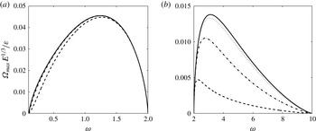
 ${\it\Omega}_{\mathit{max}}=h_{o}{\it\varepsilon}E^{-1/3}v_{1}{\it\alpha}^{-5/6}$
, with
 $h_{0}\approx 0.188$
. The variations of this maximum with respect to
 ${\it\omega}$
and
 $Pr$
are shown in figure 5 for both a weakly stratified and a strongly stratified case. Whatever the value of
 $N$
, the maximum angular velocity is found to increase with
 $Pr$
, with a maximum reached for
 $Pr=\infty$
. The function
 ${\it\Omega}_{\mathit{max}}$
is also found to reach a maximum value within the inertia-gravity frequency range far from its boundaries where it vanishes. Interestingly, one can note that the weakly stratified case (
 $N=0.1$
) provides larger amplitudes than the strongly stratified case (
 $N=10$
).
Variation of the maximum angular velocity of the harmonic response with respect to
 ${\it\omega}$
for
 $N=0.1$
(a) and
 $N=10$
(b). Solid line,
 $Pr=\infty$
; dotted line,
 $Pr=10$
; dash–dot line,
 $Pr=1$
; dashed line,
 $Pr=0.1$
.

The functions
 $\text{H}_{+}^{(m,n)}$
and
 $\text{H}_{-}^{(m,n)}$
describing the spatial structure of the harmonic response close to the focus point satisfy the properties that
 $$\begin{eqnarray}\text{H}_{-}^{(m,n)}(R,Z)=(\text{H}_{+}^{(m,n)}(R,Z))^{\ast }=\text{H}_{+}^{(m,n)}(R,-Z),\end{eqnarray}$$
so the entire time evolution can be deduced from the case
 ${\it\epsilon}_{1}=1$
in a quarter of a period. If we define
 $t_{o}$
such that
 $-{\it\omega}t_{o}+{\it\phi}_{v_{1}}+{\it\epsilon}_{1}{\rm\pi}/4+{\rm\pi}=0$
, and use an adequate normalization, we can write the velocity and buoyancy fields as
 $$\begin{eqnarray}\displaystyle \displaystyle \bar{v}_{r} & = & \displaystyle {\it\epsilon}_{1}\text{Im}(\text{H}_{+}^{(1,1)}(R,Z))\cos ({\it\omega}(t-t_{o}))+\text{Re}(\text{H}_{+}^{(1,1)}(R,Z))\sin ({\it\omega}(t-t_{o})),\end{eqnarray}$$
 $$\begin{eqnarray}\displaystyle \displaystyle \bar{v}_{{\it\theta}} & = & \displaystyle \text{Re}(\text{H}_{+}^{(1,1)}(R,Z))\cos ({\it\omega}(t-t_{o}))-\,{\it\epsilon}_{1}\text{Im}(\text{H}_{+}^{(1,1)}(R,Z))\sin ({\it\omega}(t-t_{o})),\end{eqnarray}$$
 $$\begin{eqnarray}\displaystyle \displaystyle \bar{v}_{z} & = & \displaystyle {\it\epsilon}_{1}\text{Re}(\text{H}_{+}^{(1,0)}(R,Z))\cos ({\it\omega}(t-t_{o}))-\text{Im}(\text{H}_{+}^{(1,0)}(R,Z))\sin ({\it\omega}(t-t_{o})),\end{eqnarray}$$
 $$\begin{eqnarray}\displaystyle \displaystyle \bar{B} & = & \displaystyle -\text{Im}(\text{H}_{+}^{(1,0)}(R,Z))\cos ({\it\omega}(t-t_{o}))-{\it\epsilon}_{1}\text{Re}(\text{H}_{+}^{(1,0)}(R,Z))\sin ({\it\omega}(t-t_{o})).\qquad\end{eqnarray}$$
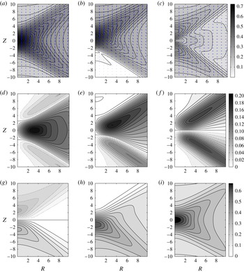
Time evolution of the velocity field and buoyancy field close to the focus point for
 ${\it\epsilon}_{1}=1$
. (a–c) Vector fields
 $(\bar{v}_{r},\bar{v}_{z})$
and contour levels of
 $\sqrt{\bar{v}_{r}^{2}+\bar{v}_{i}^{2}}$
. (d–f) Contour levels of
 $\bar{v}_{{\it\theta}}$
. (g–i) Contour levels of
 $\bar{B}$
. Here,
 ${\it\omega}(t-t_{o})=(a\text{,}d\text{,}g)~0,(b\text{,}e\text{,}h)~{\rm\pi}/4,(c\text{,}f\text{,}i)~{\rm\pi}/2$
.

4. Mean flow correction
In this section, we calculate the mean flow correction generated by the nonlinear interaction of the harmonic flow with itself. As for the harmonic components, we focus on the limit of small Ekman numbers for which simpler expressions are obtained. The two small parameters
 $E$
and
 ${\it\varepsilon}$
are independent. However, by construction, the limit
 ${\it\varepsilon}\rightarrow 0$
is performed first.
The mean flow is forced by the Reynolds stress (right-hand side of (2.6)), whose amplitude varies strongly according to the position. In the bulk, far from the disk boundary and far from
 $L_{j}$
when
 ${\it\omega}\in I_{{\it\omega}}$
, the velocity components are
 $O({\it\varepsilon}\sqrt{E})$
, so the Reynolds stress is small and of order
 $O({\it\varepsilon}^{2}E)$
. In the boundary layer of the librating disk, the Reynolds stress is
 $O({\it\varepsilon}^{2})$
, whereas close to
 $L_{j}$
the Reynolds stress is
 $O({\it\varepsilon}^{2}E^{1/3})$
. At the focus point, it becomes of order
 $O({\it\varepsilon}^{2}E^{-1/3})$
, and at the disk border, it is
 $O({\it\varepsilon}^{2}E^{-1/2})$
.
In the bulk, because the mean flow correction turns out to be larger than the Reynolds stress, it has to be a homogeneous solution of (2.6a–e
). The solution of these equations can be sought in the form (3.1a–e
) with
 ${\it\omega}=0$
. When
 $N>0$
, only the ‘non-viscous contributions’ associated with
 ${\it\mu}_{1}\sim \text{i}N\sqrt{Pr}k/2$
and
 ${\it\mu}_{4}\sim \text{i}k$
are expected to be present. This gives
 $$\begin{eqnarray}\displaystyle & \displaystyle u_{0}\sim \frac{E(N^{2}Pr-4)}{8}\int _{0}^{\infty }k^{2}B_{0}(k)\text{e}^{-((N\sqrt{Pr})/2)kz}\text{J}_{1}(kr)\,\text{d}k, & \displaystyle\end{eqnarray}$$
 $$\begin{eqnarray}\displaystyle & \displaystyle v_{0}\sim \int _{0}^{\infty }\left(A_{0}(k)\text{e}^{-kz}+B_{0}(k)\text{e}^{-((N\sqrt{Pr})/2)kz}\right)\text{J}_{1}(kr)\,\text{d}k, & \displaystyle\end{eqnarray}$$
 $$\begin{eqnarray}\displaystyle & \displaystyle w_{0}\sim \frac{E(N^{2}Pr-4)}{4N\sqrt{Pr}}\int _{0}^{\infty }k^{2}B_{0}(k)\text{e}^{-((N\sqrt{Pr})/2)kz}\text{J}_{0}(kr)\,\text{d}k, & \displaystyle\end{eqnarray}$$
 $$\begin{eqnarray}\displaystyle & \displaystyle b_{0}\sim -\int _{0}^{\infty }\left(2A_{0}(k)\text{e}^{-kz}+N\sqrt{Pr}B_{0}(k)\text{e}^{-((N\sqrt{Pr})/2)kz}\right)\text{J}_{0}(kr)\,\text{d}k, & \displaystyle\end{eqnarray}$$
 $A_{0}(k)$
and
 $B_{0}(k)$
are functions prescribed by the matching with the other regions. These expressions tell us that, in the bulk, the radial and axial velocity fields are
 $O(E)$
smaller than the azimuthal velocity and buoyancy components when
 $N\neq 0$
.
When
 $N=0$
,
 ${\it\mu}_{1}=O(E)$
,
 $b_{0}=0$
and the solution is
 $$\begin{eqnarray}\displaystyle & \displaystyle u_{0}\sim -\frac{E}{2}\int _{0}^{\infty }k^{2}B_{0}(k)\text{e}^{-((k^{3}E)/2)z}\text{J}_{1}(kr)\,\text{d}k, & \displaystyle\end{eqnarray}$$
 $$\begin{eqnarray}\displaystyle & \displaystyle v_{0}\sim \int _{0}^{\infty }B_{0}(k)\text{e}^{-((k^{3}E)/2)z}\text{J}_{1}(kr)\,\text{d}k, & \displaystyle\end{eqnarray}$$
 $$\begin{eqnarray}\displaystyle & \displaystyle w_{0}\sim -\int _{0}^{\infty }B_{0}(k)\text{e}^{-((k^{3}E)/2)z}\text{J}_{0}(kr)\,\text{d}k. & \displaystyle\end{eqnarray}$$
 $A_{0}$
and
 $B_{0}$
when
 $N\neq 0$
and
 $B_{0}$
when
 $N=0$
are obtained by matching expressions (4.1a–d
) or (4.2a–c
) with the boundary layer solution, as shown in the next section.
4.1. Generation from the boundary layer
In the boundary layer, the Reynolds stress is of order
 ${\it\varepsilon}^{2}$
when
 $r<1$
, and of order
 ${\it\varepsilon}^{2}E$
for
 $r>1$
. The main contribution is then expected to come from the boundary layer on the disk (
 $r<1$
). For
 $r<1$
, the amplitudes of the mean flow correction can be written as
 $$\begin{eqnarray}\displaystyle & \displaystyle u_{0}\sim \bar{u}_{0}(\bar{z},r)+u_{0_{0}}^{(out)}(r), & \displaystyle\end{eqnarray}$$
 $$\begin{eqnarray}\displaystyle & \displaystyle v_{0}\sim \bar{v}_{0}(\bar{z},r)+v_{0_{0}}^{(out)}(r), & \displaystyle\end{eqnarray}$$
 $$\begin{eqnarray}\displaystyle & \displaystyle w_{0}\sim \sqrt{E}\bar{w}_{0}(\bar{z},r)+w_{0_{0}}^{(out)}(r), & \displaystyle\end{eqnarray}$$
 $$\begin{eqnarray}\displaystyle & \displaystyle p_{0}\sim E\bar{p}_{0}(\bar{z},r)+p_{0_{0}}^{(out)}(r), & \displaystyle\end{eqnarray}$$
 $$\begin{eqnarray}\displaystyle & \displaystyle b_{0}\sim \sqrt{E}\bar{b}_{0}(\bar{z},r)+b_{0_{0}}^{(out)}(r), & \displaystyle\end{eqnarray}$$
 $u_{0_{0}}^{(out)},v_{0_{0}}^{(out)},\ldots$
are associated with non-viscous outer (bulk) contributions within the boundary layer and
 $\bar{z}=z/\sqrt{E}$
is the boundary layer variable. From (2.6a–e
), we obtain the system
 $$\begin{eqnarray}\displaystyle & \displaystyle 2\bar{v}_{0}+\displaystyle \frac{\partial ^{2}\bar{u}_{0}}{\partial \bar{z}^{2}}=\bar{N}_{u}, & \displaystyle\end{eqnarray}$$
 $$\begin{eqnarray}\displaystyle & \displaystyle -2\bar{u}_{0}+\displaystyle \frac{\partial ^{2}\bar{v}_{0}}{\partial \bar{z}^{2}}=\bar{N}_{v}, & \displaystyle\end{eqnarray}$$
 $$\begin{eqnarray}\displaystyle & \displaystyle \displaystyle \frac{\partial ^{2}\bar{w}_{0}}{\partial \bar{z}^{2}}-\displaystyle \frac{\partial \bar{p}_{0}}{\partial \bar{z}}-\bar{b}_{0}=\bar{N}_{w}, & \displaystyle\end{eqnarray}$$
 $$\begin{eqnarray}\displaystyle & \displaystyle \displaystyle \frac{\partial ^{2}\bar{b}_{0}}{\partial \bar{z}^{2}}+N^{2}Pr\bar{w}_{0}=Pr\bar{N}_{b}, & \displaystyle\end{eqnarray}$$
 $$\begin{eqnarray}\displaystyle & \displaystyle \frac{1}{r}\displaystyle \frac{\partial r\bar{u}_{0}}{\partial r}+\displaystyle \frac{\partial \bar{w}_{0}}{\partial \bar{z}}=0, & \displaystyle\end{eqnarray}$$
 $$\begin{eqnarray}\displaystyle & \displaystyle \bar{N}_{u}=\bar{u}\displaystyle \frac{\partial \bar{u}^{\ast }}{\partial r}+\bar{w}\displaystyle \frac{\partial \bar{u}^{\ast }}{\partial \bar{z}}-\frac{|\bar{v}|^{2}}{r}+\text{c.c.}, & \displaystyle\end{eqnarray}$$
 $$\begin{eqnarray}\displaystyle & \displaystyle \bar{N}_{v}=\bar{u}\displaystyle \frac{\partial \bar{v}^{\ast }}{\partial r}+\bar{w}\displaystyle \frac{\partial \bar{v}^{\ast }}{\partial \bar{z}}+\frac{\bar{u}\bar{v}^{\ast }}{r}+\text{c.c.}, & \displaystyle\end{eqnarray}$$
 $$\begin{eqnarray}\displaystyle & \displaystyle \bar{N}_{w}=\bar{u}\displaystyle \frac{\partial \bar{w}^{\ast }}{\partial r}+\bar{w}\displaystyle \frac{\partial \bar{w}^{\ast }}{\partial \bar{z}}+\text{c.c.}, & \displaystyle\end{eqnarray}$$
 $$\begin{eqnarray}\displaystyle & \displaystyle \bar{N}_{b}=\bar{u}\displaystyle \frac{\partial \bar{b}^{\ast }}{\partial r}+\bar{w}\displaystyle \frac{\partial \bar{b}^{\ast }}{\partial \bar{z}}+\text{c.c.}, & \displaystyle\end{eqnarray}$$
 $\bar{u}$
,
 $\bar{v}$
 $\bar{w}$
and
 $\bar{b}$
are the amplitudes of the harmonic solution defined in (3.11a–d
). These equations can be solved as
 $$\begin{eqnarray}\displaystyle & \displaystyle \bar{u}_{0}=r(-b_{0}\cos (\bar{z})+a_{0}\sin (\bar{z}))\text{e}^{-\bar{z}}+r\bar{u}_{p}(\bar{z}), & \displaystyle\end{eqnarray}$$
 $$\begin{eqnarray}\displaystyle & \displaystyle \bar{v}_{0}=r(a_{0}\cos (\bar{z})+b_{0}\sin (\bar{z}))\text{e}^{-\bar{z}}+r\bar{v}_{p}(\bar{z}), & \displaystyle\end{eqnarray}$$
 $$\begin{eqnarray}\displaystyle & \displaystyle \bar{w}_{0}=((a_{0}-b_{0})\cos (\bar{z})+(a_{0}+b_{0})\sin (\bar{z}))\text{e}^{-\bar{z}}+\bar{w}_{p}(\bar{z}), & \displaystyle\end{eqnarray}$$
 $\bar{u}_{p}$
,
 $\bar{v}_{p}$
and
 $\bar{w}_{p}$
are particular solutions of the non-homogeneous equations (4.4a,b,e
) which have the same form as the nonlinear terms (i.e. sum of exponentials). In particular, they vanish at infinity and satisfy
 $\bar{u}_{p}(\bar{z})=(\partial _{\bar{z}}^{2}\bar{v}_{p}-\bar{N}_{v}/r)/2$
and
 $\bar{w}_{p}=-2\int _{+\infty }^{\bar{z}}\bar{u}_{p}(s)\,\text{d}s$
. On inserting these expressions in (4.3a–c
) and applying the no-slip boundary condition we obtain
 $$\begin{eqnarray}\displaystyle & \displaystyle r(-b_{0}+\bar{u}_{p}(0))+u_{0_{0}}^{(out)}(r)=0, & \displaystyle\end{eqnarray}$$
 $$\begin{eqnarray}\displaystyle & \displaystyle r(a_{0}+\bar{v}_{p}(0))+v_{0_{0}}^{(out)}(r)=0, & \displaystyle\end{eqnarray}$$
 $$\begin{eqnarray}\displaystyle & \displaystyle \sqrt{E}(a_{0}-b_{0}+\bar{w}_{p}(0))+w_{0_{0}}^{(out)}(r)=0. & \displaystyle\end{eqnarray}$$
 $\bar{N}_{u}$
and
 $\bar{N}_{v}$
do not depend on
 $N$
and
 $Pr$
, the particular solutions
 $\bar{u}_{p}$
,
 $\bar{v}_{p}$
and
 $\bar{w}_{p}$
are also independent of
 $N$
and
 $Pr$
and equal to the solutions obtained in the unstratified case. The above equations thus apply for both cases
 $N=0$
and
 $N\neq 0$
.
However, when
 $N\neq 0$
, the condition of matching of (4.3a–c
) with (4.1a–c
) requires that
 $u_{0_{0}}^{(out)}$
and
 $w_{0_{0}}^{(out)}$
are
 $O(E)$
smaller than
 $v_{0_{0}}^{(out)}$
. This implies that we should have, at leading order,
 $-b_{0}+\bar{u}_{p}(0)=0$
and
 $a_{0}-b_{0}+\bar{w}_{p}(0)=0$
from (4.7a,c
), which gives in (4.7b
)
 $$\begin{eqnarray}\displaystyle v_{0_{0}}^{(out)}=r(\bar{w}_{p}(0)-\bar{u}_{p}(0)-\bar{v}_{p}(0))\equiv r{\it\Omega}_{2}({\it\omega}), & & \displaystyle\end{eqnarray}$$
where the function
 ${\it\Omega}_{2}$
depends on
 ${\it\omega}$
only. This equality gives the amplitude of the azimuthal flow needed to cancel the Ekman pumping (axial flux) created by the nonlinear interactions in the boundary layer. This situation, where no axial flux is permitted in the bulk, has already been encountered in the literature for a bounded configuration without stratification. Wang (Reference Wang1970) and Sauret et al. (Reference Sauret, Cébron, Le Bars and Le Dizès2012) showed that the zonal flow created by librating a cylinder satisfies this property. As a consequence, the value of the mean angular velocity
 ${\it\Omega}_{2}$
is equal to the value obtained for a librating cylinder. It corresponds to the function
 ${\it\Omega}_{2}({\it\omega})$
given in the appendix of Sauret et al. (Reference Sauret, Cébron, Le Bars and Le Dizès2012).
Expression (4.8) tells us that the outer mean flow is a solid-body rotation close to the disk boundary (
 $r<1$
), while it is expected to vanish at this order on the boundary outside the disk (
 $r>1$
). Moreover, at this order, the buoyancy of the outer mean flow should also vanish on the disk (since the boundary layer contribution is
 $O(\sqrt{E})$
smaller). On applying these conditions of matching to (4.1b,d
) we obtain, using the property (3.5), the following equalities for the amplitudes
 $A_{0}(k)$
and
 $B_{0}(k)$
of the solution in the bulk:
 $$\begin{eqnarray}\displaystyle & A_{0}(k)+B_{0}(k)={\it\Omega}_{2}\text{J}_{2}(k), & \displaystyle\end{eqnarray}$$
 $$\begin{eqnarray}\displaystyle & 2A_{0}(k)+N\sqrt{Pr}B_{0}(k)=0. & \displaystyle\end{eqnarray}$$
 $$\begin{eqnarray}\displaystyle & \displaystyle v_{0}\sim {\it\Omega}_{2}\int _{0}^{+\infty }\frac{2\text{e}^{-((N\sqrt{Pr})/2)kz}-N\sqrt{Pr}\text{e}^{-kz}}{2-N\sqrt{Pr}}\text{J}_{2}(k)\text{J}_{1}(kr)\,\text{d}k, & \displaystyle\end{eqnarray}$$
 $$\begin{eqnarray}\displaystyle & \displaystyle b_{0}\sim -{\it\Omega}_{2}\frac{2N\sqrt{Pr}}{2-N\sqrt{Pr}}\int _{0}^{+\infty }\left(\text{e}^{-((N\sqrt{Pr})/2)kz}-\text{e}^{-kz}\right)\text{J}_{2}(k)\text{J}_{0}(kr)\,\text{d}k. & \displaystyle\end{eqnarray}$$
 $v_{0}$
and
 $b_{0}$
therefore depends on a single parameter
 ${\it\Lambda}=N\sqrt{Pr}/2$
and can be written as
 $$\begin{eqnarray}\displaystyle & \displaystyle v_{0}\sim {\it\Omega}_{2}\frac{G^{(1)}(r,{\it\Lambda}z)-{\it\Lambda}G^{(1)}(r,z)}{1-{\it\Lambda}}, & \displaystyle\end{eqnarray}$$
 $$\begin{eqnarray}\displaystyle & \displaystyle b_{0}\sim -2{\it\Omega}_{2}{\it\Lambda}\frac{G^{(0)}(r,{\it\Lambda}z)-G^{(0)}(r,z)}{1-{\it\Lambda}}, & \displaystyle\end{eqnarray}$$
 $$\begin{eqnarray}\displaystyle G^{(n)}(r,z)=\int _{0}^{+\infty }\text{J}_{2}(k)\text{J}_{n}(kr)\text{e}^{-kz}\,\text{d}k. & & \displaystyle\end{eqnarray}$$
It should be noted that when
 ${\it\Lambda}\rightarrow \infty$
, that is when there is no buoyancy diffusion (
 $Pr\gg 1$
) or when the fluid is strongly stratified (
 $N\gg 1$
), we obtain even simpler expressions:
 $$\begin{eqnarray}\displaystyle v_{0}\sim {\it\Omega}_{2}G^{(1)}(r,z),\quad b_{0}\sim -2{\it\Omega}_{2}G^{(0)}(r,z). & & \displaystyle\end{eqnarray}$$
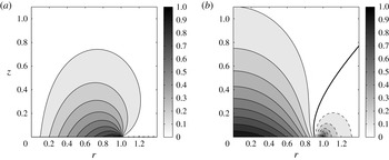
The contours of the functions
 $G^{(1)}(r,z)$
and
 $G^{(0)}(r,z)$
are plotted in figure 7. It should be noted that the zonal flow generated by the boundary layer extends to at least an
 $O(1)$
region above the disk, even in the strongly stratified case. Moreover, the zonal flow structure does not depend on the frequency, which means that the same zonal flow is obtained whether
 ${\it\omega}\in I_{{\it\omega}}$
or not.
The mean flow correction in the bulk generated by the boundary layer with stratification. Contours in the
 $(r,z)$
plane of the functions
 $G^{(1)}(r,z)$
(a) and
 $G^{(0)}(r,z)$
(b) characterizing the azimuthal mean flow correction and the mean buoyancy correction respectively. In (b) the grey levels are for the norm of
 $G^{(0)}$
, and the solid and dashed lines are for positive and negative values of
 $G^{(0)}$
respectively.

When
 $N=0$
, an axial flux from the boundary layer is possible, and the form (4.2a–c
) of the solution in an open domain implies that
 $v_{0}^{(out)}(0)$
and
 $w_{0}^{(out)}(0)$
are of the same order. This is possible while satisfying (4.7a–c
) only if
 $-b_{0}+\bar{u}_{p}(0)=0$
and
 $a_{0}+\bar{v}_{p}(0)=0$
, which gives
 $$\begin{eqnarray}\displaystyle w_{0}^{(out)}(0)=\sqrt{E}(\bar{u}_{p}(0)+\bar{v}_{p}(0)-\bar{w}_{p}(0))=-\sqrt{E}\,{\it\Omega}_{2}. & & \displaystyle\end{eqnarray}$$
This equality is obtained for
 $r<1$
. Keeping in mind that at this order
 $w_{0}^{(out)}(0)=0$
for
 $r>1$
, and that (Watson Reference Watson1952, P406)
 $$\begin{eqnarray}\displaystyle \int _{0}^{\infty }\text{J}_{1}(k)\text{J}_{0}(kr)\,\text{d}k=\text{H}(1-r), & & \displaystyle\end{eqnarray}$$
we immediately deduce, from the condition of matching of (4.3c ) with (4.2c ), that
 $$\begin{eqnarray}\displaystyle B_{0}(k)=-\sqrt{E}\,{\it\Omega}_{2}\text{J}_{1}(k). & & \displaystyle\end{eqnarray}$$
Expressions (4.2b,c
) then give when
 $z\ll 1/E$
 $$\begin{eqnarray}\displaystyle & v_{0}\sim -\sqrt{E}\,{\it\Omega}_{2}\,g_{1}(r), & \displaystyle\end{eqnarray}$$
 $$\begin{eqnarray}\displaystyle & w_{0}\sim -\sqrt{E}\,{\it\Omega}_{2}\,g_{0}(r), & \displaystyle\end{eqnarray}$$
 $$\begin{eqnarray}\displaystyle g_{n}(r)=\int _{0}^{\infty }\text{J}_{1}(k)\text{J}_{n}(kr)\,\text{d}k. & & \displaystyle\end{eqnarray}$$
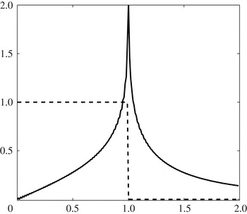
The functions
 $g_{0}(r)$
and
 $g_{1}(r)$
are plotted in figure 8. The function
 $g_{1}(r)$
diverges at
 $r=1$
, which means that viscosity has a significant role close to the line
 $r=1$
in smoothing the singularity. It leads to a mean azimuthal velocity of order
 ${\it\varepsilon}^{2}\sqrt{E}\ln (E)$
. We suspect that a larger contribution could exist corresponding to a Dirac source of axial flow at the edge of the disk at
 $r=1$
. We have seen that such a contribution does exist for the harmonic response. Here, it would give a function
 $B_{0}(k)$
proportional to
 $k\text{J}_{0}(k)$
(Tilgner Reference Tilgner2000), leading to an
 $O({\it\varepsilon}^{2}E^{1/6})$
contribution close to the line
 $r=1$
, with the same typical Scorer function for its transverse spatial structure as for the harmonic response.
The mean flow correction in the bulk generated by the boundary layer without stratification (
 $N=0$
). Plot of the functions
 $g_{0}(r)$
(dashed line) and
 $g_{1}(r)$
(solid line) characterizing the axial mean flow and the azimuthal mean flow respectively.

4.2. Close to the singularity lines
In the previous section, we have calculated the mean flow correction in the bulk generated by the nonlinear interaction in the boundary layer. When
 ${\it\omega}\in I_{{\it\omega}}$
, another contribution of order
 ${\it\varepsilon}^{2}E^{1/3}$
is also created close to the singularity lines
 $L_{j}$
.
When
 $N\neq 0$
, the azimuthal velocity and buoyancy fields associated with this correction are negligible compared with the
 $O({\it\varepsilon}^{2})$
contributions coming from the boundary layer (see expressions (4.11a,b
)). The radial and axial velocity components of this mean flow correction are, by contrast, expected to be dominant. These velocity fields are associated with a mean flow correction aligned along with the line
 $L_{j}$
. They are obtained from (2.6b,e
), which give
 $$\begin{eqnarray}\displaystyle & u_{0}=E^{1/3}\tilde{u} _{0}, & \displaystyle\end{eqnarray}$$
 $$\begin{eqnarray}\displaystyle & \displaystyle w_{0}={\it\epsilon}_{0}E^{1/3}\displaystyle \frac{\tilde{u} _{0}}{{\it\mu}_{1_{0}}},\quad \text{with }{\it\epsilon}_{0}=\left\{\begin{array}{@{}ll@{}}-1 & \text{on}~L_{1},\\ +1 & \text{on}~L_{2}~\text{and}~L_{3},\end{array}\right. & \displaystyle\end{eqnarray}$$
 $$\begin{eqnarray}\displaystyle 2{\it\Omega}_{0}\tilde{u} _{0}=-{\tilde{N}}_{v}=-\left(\displaystyle \frac{\partial \tilde{v}_{\Vert }\tilde{v}^{\ast }}{\partial {\it\eta}_{\Vert }}+\displaystyle \frac{\partial \tilde{v}_{\bot }\tilde{v}^{\ast }}{\partial {\it\eta}_{\bot }}+\frac{\tilde{v}_{\Vert }\tilde{v}^{\ast }}{r}+\text{c.c.}\right)=-\!\left(\displaystyle \frac{\partial \tilde{v}_{\bot }\tilde{v}^{\ast }}{\partial {\it\eta}_{\bot }}+\text{c.c.}\right), & & \displaystyle\end{eqnarray}$$
where
 $\tilde{v}$
and
 $\tilde{v}_{\bot }$
are given by (3.31a
) and (3.33). It should be noted that the simplification in (4.20) is due to the phase quadrature between
 $v_{\Vert }$
and
 $v$
.
When
 $N=0$
, the mean flow generated close to the line
 $L_{j}$
is the dominant contribution as the boundary layer contribution is
 $O({\it\varepsilon}^{2}E^{1/2})$
. The radial and axial components are still given by (4.19a,b
) and (4.20). If we write the amplitude of the azimuthal velocity as
 $v_{0}=E^{1/3}\tilde{v}_{0}$
, we obtain, from (2.6a,c
), after having computed the pressure terms, the simple expression
 $$\begin{eqnarray}\displaystyle \tilde{v}_{0}=-\frac{|\tilde{v}|^{2}}{r}, & & \displaystyle\end{eqnarray}$$
where
 $\tilde{v}$
is given by (3.31a
).
All of the expressions obtained for the mean flow correction components go to zero far away from the line
 $L_{j}$
(that is, when
 $|{\it\eta}_{\bot }|\rightarrow \infty$
). This implies that the contribution at this order does not force any mean flow correction in the outer region away from
 $L_{j}$
. One could show that such a forcing appears at the next order, leading to a bulk contribution of order
 ${\it\varepsilon}^{2}E^{2/3}$
, which is always smaller than the contribution generated from the boundary layer.
4.3. At the focus point
Close to the focus point, the Reynolds stress scales as
 ${\it\varepsilon}^{2}E^{-1/3}$
and generates a mean flow correction of same order. We provide in this subsection the asymptotic analysis which permits us to calculate the mean flow correction.
We start with the case
 $N=0$
which is simpler. For
 $N=0$
, we can use the ansatz
 $$\begin{eqnarray}\displaystyle & u_{0}=E^{-1/3}{\check{u}}_{0}, & \displaystyle\end{eqnarray}$$
 $$\begin{eqnarray}\displaystyle & v_{0}=E^{-1/3}\check{v}_{0}, & \displaystyle\end{eqnarray}$$
 $$\begin{eqnarray}\displaystyle & w_{0}=E^{-1/3}\check{w}_{0}, & \displaystyle\end{eqnarray}$$
 $$\begin{eqnarray}\displaystyle & p_{0}=\check{p}_{1}. & \displaystyle\end{eqnarray}$$
 $R=r/\tilde{E}^{1/3}$
and
 $Z=({\it\mu}_{1_{0}}z-1)/\tilde{E}^{1/3}$
the system
 $$\begin{eqnarray}\displaystyle & \displaystyle 2\check{v}_{0}-\frac{\partial _{R}\check{p}_{1}}{{\it\alpha}^{1/3}}=\frac{1}{{\it\alpha}^{1/3}}(u\partial _{R}u^{\ast }+{\it\mu}_{1_{0}}w\partial _{Z}u^{\ast }-|v|^{2}/R+\text{c.c.})\equiv {\check{N}}_{u_{0}}, & \displaystyle\end{eqnarray}$$
 $$\begin{eqnarray}\displaystyle & \displaystyle -2{\check{u}}_{0}=\frac{1}{{\it\alpha}^{1/3}}(u\partial _{R}v^{\ast }+{\it\mu}_{1_{0}}w\partial _{Z}v^{\ast }-uv^{\ast }/R+\text{c.c.})\equiv {\check{N}}_{v_{0}}, & \displaystyle\end{eqnarray}$$
 $$\begin{eqnarray}\displaystyle & \displaystyle -\frac{{\it\mu}_{1_{0}}\partial _{Z}\check{p}_{1}}{{\it\alpha}^{1/3}}=\frac{1}{{\it\alpha}}(u\partial _{R}w^{\ast }+{\it\mu}_{1_{0}}w\partial _{Z}w^{\ast }+\text{c.c.})\equiv {\check{N}}_{w_{0}}, & \displaystyle\end{eqnarray}$$
 $$\begin{eqnarray}\displaystyle & \displaystyle \bar{\partial }_{R}{\check{u}}_{0}+{\it\mu}_{1_{0}}\partial _{Z}\check{w}_{0}=0, & \displaystyle\end{eqnarray}$$
 ${\it\mu}_{1_{0}}$
and
 ${\it\alpha}$
have been defined in (3.8a
) and
 $\bar{\partial }_{R}=\partial _{R}+1/R$
. Since
 ${\check{N}}_{v_{0}}$
reduces to
 $$\begin{eqnarray}\displaystyle {\check{N}}_{v_{0}}=\frac{{\it\mu}_{1_{0}}}{{\it\alpha}^{1/3}}\partial _{Z}(wv^{\ast }+vw^{\ast }), & & \displaystyle\end{eqnarray}$$
we immediately get from (4.23b,d )
 $$\begin{eqnarray}\displaystyle & \displaystyle {\check{u}}_{0}=-\frac{{\it\mu}_{1_{0}}}{2{\it\alpha}^{1/3}}\partial _{Z}(wv^{\ast }+w^{\ast }v), & \displaystyle\end{eqnarray}$$
 $$\begin{eqnarray}\displaystyle & \displaystyle \check{w}_{0}=\frac{1}{2{\it\alpha}^{1/3}}\bar{\partial }_{R}(wv^{\ast }+w^{\ast }v). & \displaystyle\end{eqnarray}$$
 $$\begin{eqnarray}\displaystyle {\check{u}}_{0}=\frac{{\it\epsilon}_{1}|v_{1}|^{2}{\it\omega}}{4{\it\alpha}^{4/3}}U_{f}(R,Z),\quad \check{w}_{0}=\frac{{\it\epsilon}_{1}|v_{1}|^{2}{\it\omega}}{4{\it\mu}_{1_{0}}{\it\alpha}^{4/3}}W_{f}(R,Z), & & \displaystyle\end{eqnarray}$$
with
 $$\begin{eqnarray}\displaystyle & U_{f}(R,Z)=\text{Im}(\text{H}_{+}^{(2,0)}\text{H}_{-}^{(1,1)}-\text{H}_{+}^{(1,0)}\text{H}_{-}^{(2,1)}), & \displaystyle\end{eqnarray}$$
 $$\begin{eqnarray}\displaystyle & W_{f}(R,Z)=\text{ Re }(\text{H}_{+}^{(2,0)}\text{H}_{-}^{(1,0)}-\text{H}_{+}^{(1,1)}\text{H}_{-}^{(2,1)}), & \displaystyle\end{eqnarray}$$
 $\text{H}_{{\it\epsilon}_{1}}^{(m,n)}(R,Z)$
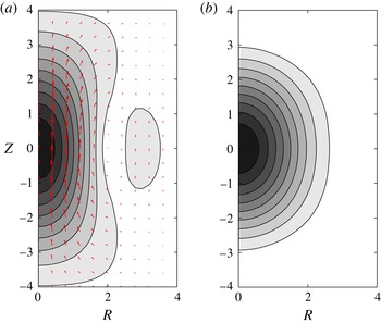
has been defined in (3.36). In figure 9(a), we have plotted the contours of
 $\sqrt{U_{f}^{2}+W_{f}^{2}}$
together with the vector field
 $(U_{f},W_{f})$
in a meridional plane. It should be noted that the mean poloidal flow corresponds to a flow oriented upward when
 ${\it\epsilon}_{1}=1$
and downward when
 ${\it\epsilon}_{1}=-1$
. The maximum of the mean poloidal field is reached at the focus point
 $(R,Z)=(0,0)$
and has a maximum amplitude which is for
 $N=0$
 $$\begin{eqnarray}\displaystyle w_{0}^{\mathit{max}}=E^{-1/3}h_{1}\frac{{\it\omega}^{4/3}(4-{\it\omega}^{2})^{7/6}}{2^{1/3}~32},\quad \text{with}~h_{1}=\max \left(\sqrt{U_{f}^{2}+W_{f}^{2}}\right)\approx 0.222. & & \displaystyle\end{eqnarray}$$
The azimuthal velocity field can be obtained from (4.23a,c ) which give, after eliminating the pressure,
 $$\begin{eqnarray}\displaystyle 2{\it\mu}_{1_{0}}\partial _{Z}\check{v}_{0}={\it\mu}_{1_{0}}\partial _{Z}{\check{N}}_{u_{0}}-\partial _{R}{\check{N}}_{w_{0}}\equiv {\check{N}}_{1}, & & \displaystyle\end{eqnarray}$$
where
 ${\check{N}}_{1}$
reduces, using (3.37), to
 $$\begin{eqnarray}\displaystyle {\check{N}}_{1}=\displaystyle \frac{2|v_{1}|^{2}}{{\it\alpha}^{4/3}}\displaystyle \frac{\partial }{\partial Z}\left[\frac{(1+{\it\mu}_{1_{0}}^{2}){\it\omega}^{2}}{4{\it\mu}_{1_{0}}^{2}}Re\left(\text{H}_{+}^{(2,1)}\text{H}_{-}^{(1,0)}-\displaystyle \frac{|\text{H}_{+}^{(1,1)}|^{2}}{R}\right)-\displaystyle \frac{|\text{H}_{+}^{(1,1)}|^{2}}{R}\right]. & & \displaystyle\end{eqnarray}$$
Taking
 $N=0$
, we immediately obtain
 $$\begin{eqnarray}\displaystyle \check{v}_{0}=\displaystyle \frac{{\it\omega}^{1/3}(4-{\it\omega}^{2})^{7/6}}{2^{1/3}8}V_{f}(R,Z), & & \displaystyle\end{eqnarray}$$
with
 $$\begin{eqnarray}\displaystyle V_{f}(R,Z)=Re(\text{H}_{+}^{(2,1)}\text{H}_{-}^{(1,0)})-2\displaystyle \frac{|\text{H}_{+}^{(1,1)}|^{2}}{R}. & & \displaystyle\end{eqnarray}$$
This expression is always positive, which implies that the azimuthal mean flow correction is cyclonic. It corresponds to an angular rotation localized around the focus point (see figure 9 b). The maximum angular velocity is reached at the focus point and is found to be
 $$\begin{eqnarray}\displaystyle {\it\Omega}_{0}^{\mathit{max}}=E^{-2/3}h_{2}\displaystyle \frac{{\it\omega}^{2/3}(4-{\it\omega}^{2})^{11/6}}{2^{2/3}16},\quad \text{with}~h_{2}=\max (V_{f}/R)\approx 0.0206. & & \displaystyle\end{eqnarray}$$
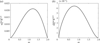
The amplitude of the zonal flow is characterized by the expressions (4.28) and (4.33), which are plotted as a function of
 ${\it\omega}$
in figure 10. On these plots, we can observe that the zonal flow vanishes at the ends of the inertia-gravity frequency range, and reaches a maximum close to the middle of the interval. The amplitudes are relatively small, but we have to keep in mind that they have been renormalized by powers of the Ekman number.
The zonal flow spatial structure. (a) The mean poloidal velocity field. Vector fields
 $(U_{f},W_{f})$
and contour levels of
 $\sqrt{U_{f}^{2}+W_{f}^{2}}$
, normalized by
 $\max \left(\sqrt{U_{f}^{2}+W_{f}^{2}}\right)\approx 0.222$
, plotted here for
 $N<2$
(
 ${\it\epsilon}=1$
). (b) The mean toroidal field. Contours of the mean angular velocity
 $V_{f}/R$
, normalized by
 $\max (V_{f}/R)\approx 0.0206$
. The same colourbar has been used for each plot, with contours every 0.1.

Variation with respect to
 ${\it\omega}$
of the maximum axial velocity (a) and the maximum angular velocity (b) of the mean flow correction for
 $N=0$
.

When
 $N\neq 0$
, the derivation of the mean flow correction is more involved. The same ansatz (4.22) can be used for the velocity and pressure fields but we should add the ansatz
 $b_{0}=E^{-1/3}\check{b}_{0}$
for the amplitude of the buoyancy correction. Insertion of these expressions in (2.6a–e
) written using the local variables leads again to (4.23a,d
) for
 ${\check{u}}_{0}$
and
 $\check{w}_{0}$
. This implies that the expressions (4.26) for
 ${\check{u}}_{0}$
and
 $\check{w}_{0}$
are still valid. In the presence of stratification, the spatial structure of the poloidal field of the mean flow correction is then the same as without stratification and is described by the functions
 $U_{f}$
and
 $W_{f}$
plotted in figure 9(a). The maximum amplitude is still reached at the focus point, but its value now depends on the Prandtl number. It goes to zero as
 $\sqrt{Pr}$
for small Prandtl number, and increases with
 $Pr$
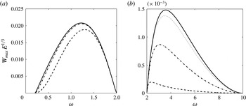
up to its maximum reached for an infinite Prandtl number. Typical variations of this maximum for a weakly stratified and a strongly stratified case are shown in figure 11. For the weakly stratified case, we are close to the results obtained without stratification, as expected. The effect of the Prandtl number turns out to be very weak for
 $Pr>1$
. For the strongly stratified case, the effect of the Prandtl number is stronger, but the amplitudes are found to be 10 times smaller than without stratification.
Variation of the maximum axial velocity of the mean flow correction with respect to
 ${\it\omega}$
for
 $N=0.2$
(a) and
 $N=10$
(b). Solid line,
 $Pr=\infty$
; dotted line,
 $Pr=10$
; dash–dot line,
 $Pr=1$
; dashed line,
 $Pr=0.1$
.

The amplitudes
 $\check{v}_{0}$
and
 $\check{b}_{0}$
of the azimuthal velocity and buoyancy of the mean flow corrections can also be obtained from the system (2.6a–e
), but some manipulations are needed to obtain
 $$\begin{eqnarray}\displaystyle & \displaystyle \partial _{R}\check{b}_{0}+2{\it\mu}_{1_{0}}\partial _{Z}\check{v}_{0}={\check{N}}_{1}, & \displaystyle\end{eqnarray}$$
 $$\begin{eqnarray}\displaystyle & \displaystyle \bar{\partial }_{R}\bar{{\it\Delta}}\check{v}_{0}-\frac{2{\it\mu}_{1_{0}}}{N^{2}Pr}\partial _{Z}{\it\Delta}\check{b}_{0}={\check{N}}_{2}, & \displaystyle\end{eqnarray}$$
 ${\check{N}}_{1}$
given by (4.30) and
 $$\begin{eqnarray}\displaystyle {\check{N}}_{2} & = & \displaystyle \displaystyle \frac{{\it\mu}_{1_{0}}(1+{\it\mu}_{1_{0}})|v_{1}|^{2}}{Pr{\it\alpha}^{2}}\left\{(Pr-1)Re(\text{H}_{+}^{(5,1)}\text{H}_{-}^{(1,1)}-\text{H}_{+}^{(5,0)}\text{H}_{-}^{(1,0)})\right.\nonumber\\ \displaystyle & & \displaystyle +\,\left.(Pr+1)Re(\text{H}_{+}^{(4,1)}\text{H}_{-}^{(2,1)}-\text{H}_{+}^{(4,0)}\text{H}_{-}^{(2,0)})\!\right\},\end{eqnarray}$$
where
 $\bar{{\it\Delta}}=\partial _{R}\bar{\partial }_{R}+{\it\mu}_{1_{0}}^{2}\partial _{Z}^{2}$
and
 ${\it\Delta}=\bar{\partial }_{R}\partial _{R}+{\it\mu}_{1_{0}}^{2}\partial _{Z}^{2}$
. These equations could a priori be solved using Hankel transform. However, the result is not sufficiently simple to be useful. As for the case without stratification, the solution is found to be localized around the focus point. Thus, it does not force any mean flow correction in the outer region at this order. The mean flow correction is forced in the outer region at the next order, and is therefore
 $O(E^{1/3})$
smaller.
5. Summary of the different scalings
In the previous sections, we have provided the spatial structure of both the harmonic response and its mean flow correction. In the weakly nonlinear regime that we have considered, which assumes a small libration amplitude
 ${\it\varepsilon}$
, the harmonic response and the mean flow correction are proportional to
 ${\it\varepsilon}$
and
 ${\it\varepsilon}^{2}$
respectively. However, they exhibit a complex dependence with respect to the Ekman number
 $E$
. The scaling in
 $E$
has been found to depend on the location and the frequency, as summarized in figures 12 and 13, which display the role of the St Andrew’s cone through the disk rim.
The Ekman scaling of the harmonic response amplitude in the meridional plane
 $(r,\tilde{z})$
(where
 $\tilde{z}=z\sqrt{|N^{2}-{\it\omega}^{2}|/|{\it\omega}^{2}-4|}$
). (a) When the frequency is in the inertia-gravity range (
 $\min (2,N)<{\it\omega}<\max (2,N)$
; (b) when the frequency is outside the inertia-gravity range (
 ${\it\omega}>\max (2,N)$
or
 ${\it\omega}<\min (2,N)$
). We have indicated in red the Ekman scaling of the width for the different regions in (a).

The results are simpler for the harmonic response (figure 12) than for the mean flow correction (figure 13). When
 ${\it\omega}\notin I_{{\it\omega}}$
, the harmonic response is
 $O(1)$
in the boundary layer of width
 $E^{1/2}$
on the disk. Elsewhere, the harmonic response is
 $O(E^{1/2})$
with a spatial structure independent of
 $N$
,
 ${\it\omega}$
and
 $Pr$
, albeit with rescaling factors that are functions of
 $N$
and
 ${\it\omega}$
. When
 ${\it\omega}\in I_{{\it\omega}}$
, the harmonic response is also
 $O(1)$
in the region of radius
 $O(E^{1/3})$
around the focus point of the singularity lines. We have seen that the spatial structure of the harmonic response near this point, as well as in the region of width
 $O(E^{1/3})$
around the singularity lines, has a universal form that does not depend on any parameter. The maximum amplitude, however, depends on
 ${\it\omega}$
and
 $N$
as well as on
 $Pr$
when
 $N\neq 0$
.
Contrary to the harmonic response, the spatial structure of the mean flow correction strongly depends on whether
 $N$
is null or not. We report in figure 13 the scaling in
 $E$
of the mean flow correction for the unstratified case (a,c) and the stratified case (b,d). The first important difference comes from the generation of the mean flow correction in the boundary layer. In the unstratified case (
 $N=0$
), we have seen that the mean flow generation is weak as the nonlinear interactions in the disk boundary layer only induce
 $O(E^{1/2})$
mean flow correction in the bulk. The mean flow generation in the boundary layer is larger when the stratification is present: it leads to an
 $O(1)$
azimuthal flow in the bulk whose spatial structure only depends on the parameter
 ${\it\Lambda}=N\sqrt{Pr}/2$
, and not on the frequency. The peculiar structure of the harmonic response is recovered in the scaling of the mean flow correction when
 ${\it\omega}\in I_{{\it\omega}}$
. Along the singularity lines, the nonlinear interactions generate an
 $O(E^{1/3})$
mean flow that is larger than the mean flow created in the boundary layer in the unstratified case. At the focus point, the mean flow correction becomes large, of order
 $E^{-1/3}$
. We have been able to compute the universal structure of this mean flow for
 $N=0$
. For
 $N\neq 0$
, we have also shown that the poloidal flow possesses the same spatial structure as for
 $N=0$
. However, the azimuthal flow is different. For both cases, the large azimuthal velocity field at the focus point implies an even larger angular velocity and vorticity field near this point. We indeed expect an
 $O({\it\varepsilon}^{2}E^{-2/3})$
vorticity field for the mean flow correction. Both the focus point region and the disk edge region are also expected to create a mean flow correction in the bulk, in regions that have the form of a Taylor–Proudman column when
 $N=0$
. We argued that they could be of order
 $E^{1/6}$
from the disk edge, and of order 1 from the focus point.
The Ekman scaling of the mean flow correction amplitude in the meridional plane
 $(r,\tilde{z})$
when
 ${\it\omega}\in I_{{\it\omega}}$
(a,b) and when
 ${\it\omega}\notin I_{{\it\omega}}$
(c,d). In (a,c)
 $N=0$
and in (b,d)
 $N\neq 0$
. We have indicated in red the Ekman scaling of the widths of the different regions.

6. Discussion
We have provided the structure of the wave field and its mean flow correction in a rotating and stratified fluid. Both stratified and non-stratified configurations have been considered, demonstrating that stratification only acts on the structure of the mean flow correction. As all temporal scales have been normalized by the rotation rate of the rotating frame, rotation has always been assumed to be present. When the rotation vanishes the flow structure becomes completely different. Indeed, without rotation, there exists a simple exact solution of the librating disk problem, which is (in dimensional form)
 $$\begin{eqnarray}\displaystyle & \displaystyle v_{r}^{\ast }=v_{z}^{\ast }=B^{\ast }=0, & \displaystyle\end{eqnarray}$$
 $$\begin{eqnarray}\displaystyle & \displaystyle v_{{\it\theta}}^{\ast }=\left\{\begin{array}{@{}ll@{}}\displaystyle {\it\varepsilon}^{\ast }r^{\ast }\text{e}^{-\sqrt{({\it\omega}^{\ast }/(2{\it\nu}^{\ast }))}z^{\ast }}\cos \left(\sqrt{\frac{{\it\omega}^{\ast }}{2{\it\nu}^{\ast }}}z^{\ast }-{\it\omega}^{\ast }t^{\ast }\right), & r^{\ast }<a^{\ast },\\ 0, & r^{\ast }>a^{\ast }.\end{array}\right. & \displaystyle\end{eqnarray}$$
This shows the essential role of the rotation in the wave field generation process. To be efficient, the generation process requires Ekman pumping to transmit the boundary layer oscillations into the bulk. We have seen that Ekman pumping does provide the source terms of the inertia-gravity wave field. Moreover, we have shown that these source terms are exactly the sum of a uniform vertical flow on the disk and of a Dirac source of vertical flow at the disk edge. Both have an amplitude equal to
 $$\begin{eqnarray}\displaystyle {\it\varepsilon}^{Ring}={\it\varepsilon}\sqrt{E}\frac{{\it\omega}|v_{1}|}{2|{\it\mu}_{1_{0}}|}, & & \displaystyle\end{eqnarray}$$
which reduces to
 $$\begin{eqnarray}\displaystyle {\it\varepsilon}^{Ring}=\frac{{\it\varepsilon}\sqrt{E}}{|4-{\it\omega}^{2}|^{1/2}}\left\{\begin{array}{@{}ll@{}}1, & {\it\omega}<2,\\ \displaystyle \frac{\sqrt{{\it\omega}+2}-\sqrt{{\it\omega}-2}}{2}, & {\it\omega}>2.\end{array}\right. & & \displaystyle\end{eqnarray}$$
We can check that this amplitude goes to zero in the weak rotation limit (
 ${\it\omega}\rightarrow \infty$
). It should be noted also that this expression diverges when
 ${\it\omega}\rightarrow 2$
. For this value of
 ${\it\omega}$
, one of the viscous wavenumbers goes to zero. The whole structure of the solution is then expected to be different. We leave this interesting limit for a future study.
It is worth mentioning that the source of the wave field does not depend on stratification, which is consistent with the form of the velocity field in the boundary layer. The amplitude of the source has the classical
 $E^{1/2}$
Ekman pumping scaling. Despite the weak amplitude of this forcing, we have seen than it generates an
 $O({\it\varepsilon})$
harmonic response and an
 $O({\it\varepsilon}^{2}E^{-1/3})$
mean flow correction. These large amplitudes are obtained at the point of focus of the singularity lines when
 ${\it\omega}\in I_{{\it\omega}}$
. Interestingly, we have observed that the structure and amplitude of the solution near this point are only related to the Dirac source at the edge of the disk. The contribution from the other source (uniform flow on the disk) has been found to be negligible close to the singularity lines, and in the neighbourhood of the point of focus. This has an important consequence: it implies that the flow structure that we have described along the singularity lines and at the focus point is the general flow structure associated with a Dirac ring source. All of the results obtained for the harmonic response and for its mean flow correction in the neighbourhood of the singularity lines and of the focus point are thus expected to apply to a general Dirac ring source.
It is therefore interesting to renormalize the results by the amplitude of the ring source to be able to consider configurations where the amplitude of the source is not related to Ekman pumping. For the harmonic response, we obtain that close to the singularity lines, using (3.31a–c
) and (3.32), the buoyancy, azimuthal and parallel velocity fields all have the same spatial structure
 $L_{{\it\epsilon}_{1}}({\it\eta}_{\bot },{\it\zeta})/\sqrt{r}$
, but with different amplitudes given by
 $$\begin{eqnarray}\frac{B^{Ring}}{{\it\varepsilon}^{Ring}}=\frac{N^{2}}{2\,{\it\omega}}\sqrt{\left|\frac{{\it\omega}^{2}-4}{N^{2}-4}\right|}\tilde{E}^{-1/3},\quad \frac{V_{{\it\theta}}^{Ring}}{{\it\varepsilon}^{Ring}}=\frac{1}{\,{\it\omega}}\sqrt{\left|\frac{N^{2}-{\it\omega}^{2}}{N^{2}-4}\right|}\tilde{E}^{-1/3},\quad \frac{V_{\Vert }^{Ring}}{{\it\varepsilon}^{Ring}}=\frac{1}{2}\tilde{E}^{-1/3},\end{eqnarray}$$
where
 $\tilde{E}$
is the rescaled Ekman number defined in (3.20). Close to the focus point, the amplitudes of the velocity and buoyancy fields of the harmonic response are
 $O(\tilde{E}^{-1/6})$
larger. The azimuthal velocity is then
 $O(\tilde{E}^{-1/2})$
, which gives a maximum angular velocity of the harmonic response
 $$\begin{eqnarray}\displaystyle \frac{{\it\Omega}_{\mathit{max}}^{Ring}}{{\it\varepsilon}^{Ring}}=\frac{2h_{0}}{{\it\omega}}\sqrt{\left|\frac{N^{2}-{\it\omega}^{2}}{{\it\omega}^{2}-4}\right|}\tilde{E}^{-5/6},\quad \text{with}~h_{0}\approx 0.188. & & \displaystyle\end{eqnarray}$$
The mean flow correction when rescaled by
 $({\it\varepsilon}^{Ring})^{2}$
exhibits even larger amplitudes. On the singularity lines, we obtain
 $O(\tilde{E}^{-2/3})$
amplitudes, while at the focus point, they are
 $O(\tilde{E}^{-4/3})$
, leading to angular velocity corrections of order
 $\tilde{E}^{-5/3}$
.
Our analysis has focused on the harmonic response and on the mean flow correction. It is clear that nonlinearity also generates higher harmonics of frequency
 $2{\it\omega}$
,
 $3{\it\omega}$
, etc., which possess their own wave field. These higher harmonics could become important when their frequency is within the inertia-gravity frequency range whereas
 ${\it\omega}\notin I_{{\it\omega}}$
.
As soon as the harmonic response or the mean flow correction becomes of order 1, which has the best chance to occur close to the disk edge or close to the focus point, one could imagine that local instability could develop and give rise to other excitation sources. Analysis of how nonlinearity would affect the solution could be one of the important next steps of the present study.
Acknowledgements
This work received support from the French Agence Nationale de la Recherche under the A*MIDEX grant ANR-11-IDEX-0001-02, the LABEX MEC project ANR-11-LABX-0092 and the ANR LIPSTIC project ANR-13-JS05-0004-01.
Appendix A. Asymptotic expressions of the coefficients for small Ekman numbers
In this section, we provide asymptotic expressions of the coefficients appearing in (3.1) when
 $E\rightarrow 0$
, assuming that
 $k$
,
 $Pr$
,
 $N$
and
 ${\it\omega}$
are all real positive numbers of order 1. Moreover, the frequency
 ${\it\omega}$
is also assumed to be different from 2,
 $N$
and
 $2/|Pr-1|$
.
The four coefficients
 $V_{j},j=1,2,3,4$
, of the azimuthal velocity are given by
 $$\begin{eqnarray}\displaystyle & V_{1}\sim v_{1}\sqrt{E}\,k\text{J}_{2}(k), & \displaystyle\end{eqnarray}$$
 $$\begin{eqnarray}\displaystyle & V_{2}\sim {\textstyle \frac{1}{2}}\text{J}_{2}(k), & \displaystyle\end{eqnarray}$$
 $$\begin{eqnarray}\displaystyle & V_{3}\sim {\textstyle \frac{1}{2}}\text{J}_{2}(k), & \displaystyle\end{eqnarray}$$
 $$\begin{eqnarray}\displaystyle & V_{4}\sim v_{4}Ek^{2}\text{J}_{2}(k), & \displaystyle\end{eqnarray}$$
 $$\begin{eqnarray}\displaystyle & \displaystyle v_{1}={\it\epsilon}_{1}\text{e}^{-\text{i}{\rm\pi}/4}\frac{\sqrt{N^{2}-{\it\omega}^{2}}(\sqrt{{\it\omega}-2}-\sqrt{{\it\omega}+2})}{{\it\omega}({\it\omega}^{2}-4)}, & \displaystyle\end{eqnarray}$$
 $$\begin{eqnarray}\displaystyle & \displaystyle v_{4}=-2\text{i}N^{2}\frac{(\sqrt{{\it\omega}^{2}-4}-{\it\omega}Pr)(\sqrt{{\it\omega}-2}-\sqrt{{\it\omega}+2})}{Pr^{1/2}{\it\omega}^{3/2}((Pr-1)^{2}{\it\omega}^{2}-4^{2})^{2}}, & \displaystyle\end{eqnarray}$$
 ${\it\epsilon}_{1}=\text{sgn}(2-N)$
when
 ${\it\omega}\in I_{{\it\omega}}$
and
 ${\it\epsilon}_{1}=1$
when
 ${\it\omega}\notin I_{{\it\omega}}$
. It should be noted that the phase
 ${\it\phi}_{v_{1}}$
of
 $v_{1}$
varies according to the relative position of
 ${\it\omega}$
,
 $N$
and 2 as
 $$\begin{eqnarray}2<{\it\omega}<N,\quad {\it\phi}_{v_{1}}=-\frac{{\rm\pi}}{4},\end{eqnarray}$$
 $$\begin{eqnarray}N<{\it\omega}<2,\quad {\it\phi}_{v_{1}}=\frac{{\rm\pi}}{4}-\arctan \left(\sqrt{\frac{2-{\it\omega}}{2+{\it\omega}}}\right),\end{eqnarray}$$
 $$\begin{eqnarray}{\it\omega}<\min (N,2),\quad {\it\phi}_{v_{1}}=-\frac{{\rm\pi}}{4}-\arctan \left(\sqrt{\frac{2-{\it\omega}}{2+{\it\omega}}}\right),\end{eqnarray}$$
 $$\begin{eqnarray}\max (N,2)<{\it\omega},\quad {\it\phi}_{v_{1}}=-\frac{3{\rm\pi}}{4}.\end{eqnarray}$$
The other coefficients can all be expressed in terms of
 $V_{j}$
:
 $$\begin{eqnarray}\displaystyle & \displaystyle U_{1}\sim \text{i}\frac{{\it\omega}}{2}V_{1}, & \displaystyle\end{eqnarray}$$
 $$\begin{eqnarray}\displaystyle & \displaystyle W_{1}\sim -\frac{{\it\epsilon}_{1}{\it\omega}}{2}\sqrt{\frac{{\it\omega}^{2}-4}{N^{2}-{\it\omega}^{2}}}V_{1}, & \displaystyle\end{eqnarray}$$
 $$\begin{eqnarray}\displaystyle & \displaystyle B_{1}\sim -\text{i}\frac{{\it\epsilon}_{1}N^{2}}{2}\sqrt{\frac{{\it\omega}^{2}-4}{N^{2}-{\it\omega}^{2}}}V_{1}, & \displaystyle\end{eqnarray}$$
 $$\begin{eqnarray}\displaystyle & \displaystyle U_{2}\sim \text{i}V_{2}, & \displaystyle\end{eqnarray}$$
 $$\begin{eqnarray}\displaystyle & \displaystyle W_{2}\sim -\frac{k\sqrt{E}}{\sqrt{{\it\omega}-2}}\text{e}^{-\text{i}{\rm\pi}/4}V_{2}, & \displaystyle\end{eqnarray}$$
 $$\begin{eqnarray}\displaystyle & \displaystyle B_{2}\sim -\frac{kN^{2}Pr\sqrt{E}}{(2+(Pr-1){\it\omega})\sqrt{{\it\omega}-2}}\text{e}^{\text{i}{\rm\pi}/4}V_{2}, & \displaystyle\end{eqnarray}$$
 $$\begin{eqnarray}\displaystyle & \displaystyle U_{3}\sim -\text{i}V_{3}, & \displaystyle\end{eqnarray}$$
 $$\begin{eqnarray}\displaystyle & \displaystyle W_{3}\sim \frac{k\sqrt{E}}{\sqrt{{\it\omega}+2}}\text{e}^{-\text{i}{\rm\pi}/4}V_{3}, & \displaystyle\end{eqnarray}$$
 $$\begin{eqnarray}\displaystyle & \displaystyle B_{3}\sim -\frac{kN^{2}Pr\sqrt{E}}{(2-(Pr-1){\it\omega})\sqrt{{\it\omega}+2}}\text{e}^{\text{i}{\rm\pi}/4}V_{3}, & \displaystyle\end{eqnarray}$$
 $$\begin{eqnarray}\displaystyle & \displaystyle U_{4}\sim -\text{i}\frac{(Pr-1){\it\omega}}{2}V_{4}, & \displaystyle\end{eqnarray}$$
 $$\begin{eqnarray}\displaystyle & \displaystyle W_{4}\sim \frac{k(Pr-1)\sqrt{{\it\omega}}}{2\sqrt{Pr}}\sqrt{E}\text{e}^{-\text{i}{\rm\pi}/4}V_{4}, & \displaystyle\end{eqnarray}$$
 $$\begin{eqnarray}\displaystyle & \displaystyle B_{4}\sim -\frac{\sqrt{Pr{\it\omega}}(4-(Pr-1)^{2}{\it\omega}^{2})}{2k\sqrt{E}}\text{e}^{-\text{i}{\rm\pi}/4}V_{4}. & \displaystyle\end{eqnarray}$$