1. Introduction
The variation in temperature of a liquid–gas interface results in the formation of surface tension gradients which induce tangential stresses, known as Marangoni stresses, driving flow in the vicinity of the interface. This mechanism is always present in non-isothermal interfacial flows and can be important in a great variety of technological applications. A characteristic problem where thermal Marangoni stresses play a significant role is the thermocapillary migration of drops and bubbles. Much of the work in this field has been reviewed by Subramanian (Reference Subramanian, Chhabra and Dekee1992) and Subramanian, Balasubramaniam & Wozniak (Reference Subramanian, Balasubramaniam, Wozniak and Monti2002).
The first reported study on the thermal migration of bubbles can be found in the pioneering work of Young, Goldstein & Block (Reference Young, Goldstein and Block1959). These authors conducted experiments on air bubbles in a viscous fluid heated from below and showed that under the effect of the induced Marangoni stresses small bubbles move downwards, whereas larger bubbles move in the opposite direction as buoyancy overcomes the effect of thermocapillarity. Young et al. (Reference Young, Goldstein and Block1959) also provided a theoretical description of the bubble motion assuming a spherical shape and creeping flow conditions, and were able to derive an analytical expression for the terminal velocity. Following this work, a series of theoretical analyses took into account the effect of convective heat transfer in the limit of both small and large Reynolds numbers (Subramanian Reference Subramanian1981, Reference Subramanian1983; Balasubramaniam & Subramaniam Reference Balasubramaniam and Subramaniam1996; Crespo, Migoya & Manuel Reference Crespo, Migoya and Manuel1998; Balasubramaniam & Subramanian Reference Balasubramaniam and Subramanian2000). Balasubramaniam & Chai (Reference Balasubramaniam and Chai1987) showed that the solution of Young et al. (Reference Young, Goldstein and Block1959) is an exact solution of the momentum equation for arbitrary Reynolds number, provided that convective heat transfer is negligible. These authors also calculated the small deformations of a drop from a spherical shape.
The main motivation for the aforementioned studies came from microgravity applications and buoyancy was considered to be negligible. The effect of the combined action of buoyancy and thermocapillarity was studied by Merritt, Morton & Subramanian (Reference Merritt, Morton and Subramanian1993), employing numerical simulations. Balasubramaniam (Reference Balasubramaniam1998) presented an asymptotic analysis in the limiting case of large Reynolds and Marangoni numbers, including the buoyant contribution as well as a temperature varying viscosity. It was shown that the steady migration velocity, at leading order, is a linear combination of the velocity for purely thermocapillary motion and the buoyancy-driven rising velocity. Later, Zhang, Subramanian & Balasubramaniam (Reference Zhang, Subramanian and Balasubramaniam2001) performed a theoretical analysis for small Marangoni numbers under the effect of gravity and showed that the inclusion of inertia is crucial in the development of an asymptotic solution for the temperature field. The asymptotic analysis presented by these authors is based on the assumption of a finite velocity and cannot be used for the case of a stationary bubble. The latter problem has to be analysed separately, as was done by Balasubramaniam & Subramanian (Reference Balasubramaniam and Subramanian2004). The solution of this problem is complicated by the presence of a singularity failing to satisfy the far-field condition. Yariv & Shusser (Reference Yariv and Shusser2006) introduced an exponentially small artificial bubble velocity as a regularization parameter to account for the inability of the asymptotic expansion to satisfy the condition of exact bubble equilibrium. They were able to evaluate the correction for the hydrodynamic force exerted on the bubble, including convective heat transfer; this correction was shown to be independent of the regularization parameter.
A great variety of numerical methods have been proposed to take into account the effect of surface deformation. These range from boundary-fitted grids (Chen & Lee Reference Chen and Lee1992; Welch Reference Welch1998), to the level-set method (Haj-Hariri, Shi & Borhan Reference Haj-Hariri, Shi and Borhan1997; Zhao et al. Reference Zhao, Li, Li and Li2010), the volume of fluid method (Ma & Bothe Reference Ma and Bothe2011), diffuse-interface methods (Borcia & Bestehorn Reference Borcia and Bestehorn2007) and hybrid schemes of the lattice-Boltzmann and the finite difference method (Liu et al. Reference Liu, Valocchi, Zhang and Kang2013). It was shown by Chen & Lee (Reference Chen and Lee1992) that surface deformation of gas bubbles reduces their terminal velocity considerably. The same effect was found also in the case of viscous drops by Haj-Hariri et al. (Reference Haj-Hariri, Shi and Borhan1997). Later, Welch (Reference Welch1998) demonstrated that as the capillary number increases and the bubble deformation becomes important, the bubbles do not reach a steady state terminal velocity. As was shown by Herrmann et al. (Reference Herrmann, Lopez, Brady and Raessi2008), the assumption of a quasi-steady state is also invalid for large Marangoni numbers. The latter finding was very recently confirmed by Wu & Hu (Reference Wu and Hu2012, Reference Wu and Hu2013).
Most of the studies mentioned above concern the motion of a single bubble or drop in an unconfined medium. Acrivos, Jeffrey & Saville (Reference Acrivos, Jeffrey and Saville1990) studied systems of multiple drops in the creeping flow limit and showed that the drops do not interact. However, when inertial effects are included it was shown by Nas & Tryggvason (Reference Nas and Tryggvason2003) and Nas, Muradoglu & Tryggvason (Reference Nas, Muradoglu and Tryggvason2006) that there are strong interactions between the droplets. The thermocapillary interaction between spherical drops in the creeping flow limit has been discussed by several authors (Leshansky, Lavrenteva & Nir Reference Leshansky, Lavrenteva and Nir2001; Leshansky & Nir Reference Leshansky and Nir2001). In the vicinity of a solid wall, the drop migration velocity is affected by the hydrodynamic resistance due to the presence of the wall as well as by the thermal interaction between the wall and the drop. Meyyappan & Subramanian (Reference Meyyappan and Subramanian1987) examined the motion of a gas bubble close to a rigid surface with an imposed far-field temperature gradient and found that the surface exerts weaker influence in the case of motion parallel to the surface than in the case of motion normal to the surface. Keh, Chen & Chen (Reference Keh, Chen and Chen2002) investigated the motion of a spherical drop between two parallel plane walls and found that the wall effect could accelerate or decelerate the droplet depending on the thermal conductivity of the droplet and the imposed boundary conditions at the wall. Chen, Dagan & Maldarelli (Reference Chen, Dagan and Maldarelli1991) considered the case of a spherical drop and studied thermocapillary migration inside an insulated tube with an imposed axial temperature gradient. They found that the migration velocity in the tube never exceeds the value in an infinite medium due to the hydrodynamic retarding forces that are developed.
Very recently, Mahesri, Haj-Hariri & Borhan (Reference Mahesri, Haj-Hariri and Borhan2014) extended the work of Chen et al. (Reference Chen, Dagan and Maldarelli1991) to take into account the effect of interfacial deformation. It was found that, as in the case of the spherical drop, the migration velocity of the confined drop is always lower than that of an unbounded drop. Brady, Herrmann & Lopez (Reference Brady, Herrmann and Lopez2011) presented numerical simulations of a droplet inside a rectangular box and showed that for low Marangoni numbers the drop rapidly settles to a quasi-steady state, whereas for high Marangoni numbers the initial conditions significantly affect the behaviour of the droplet. In the case of severe confinement inside a tube, the drop can become quite long. Such a case was studied by Hasan & Balasubramaniam (Reference Hasan and Balasubramaniam1989) and Wilson (Reference Wilson1993), who focused their attention on the thin film region away from the drop ends, and were able to derive a relation between the migration velocity and the film thickness. Later, Mazouchi & Homsy (Reference Mazouchi and Homsy2000, Reference Mazouchi and Homsy2001) used lubrication theory to determine the liquid film thickness and migration velocity for the case of cylindrical and polygonal tubes, respectively.
It is well known that the surface tension of common fluids, such as air, water and various oils, decreases almost linearly with increasing temperature; all of the above-mentioned studies have considered such fluids. In the present paper, we are interested in the thermocapillary migration of a deformable bubble inside a cylindrical tube filled with liquids that exhibit a non-monotonic dependence of the surface tension on temperature. In particular, these so-called ‘self-rewetting’ fluids (Vochten & Petre Reference Vochten and Petre1973; Petre & Azouni Reference Petre and Azouni1984; Limbourgfontaine, Petre & Legros Reference Limbourgfontaine, Petre and Legros1986; Savino et al. Reference Savino, Cecere and Paola2009, Reference Savino, Cecere, Vaerenbergh, Abe, Pizzirusso, Tzevelecos, Mojahed and Galand2013), which are non-azeotropic, high-carbon alcohol solutions, have quasi-parabolic surface-tension–temperature curves with well-defined minima; the parabolicity of these curves increases with alcohol concentration. These fluids were first studied by Vochten & Petre (Reference Vochten and Petre1973), who observed the occurrence of the minimum in surface tension with temperature in high-carbon alcohol solutions. Petre & Azouni (Reference Petre and Azouni1984) carried out experiments that involved imposing a temperature gradient on the surface of alcohol aqueous solutions, and used talc particles to demonstrate the unusual behaviour of these fluids. Experimental work on these fluids was also carried out under reduced-gravity conditions by Limbourgfontaine et al. (Reference Limbourgfontaine, Petre and Legros1986). The term ‘self-rewetting’ was coined by Abe, Iwasaki & Tanaka (Reference Abe, Iwasaki and Tanaka2004), who studied the thermophysical properties of dilute aqueous solution of high-carbon alcohols. Due to thermocapillary stresses, and the shape of the surface-tension–temperature curve, the fluids studied ‘self-rewet’ by spreading spontaneously towards the hot regions, thereby preventing dry-out of hot surfaces and enhancing the rate of heat transfer.
Due to the above-mentioned properties, ‘self-rewetting’ fluids were shown to be associated with substantially higher critical heat fluxes in heat pipes than for water (Mcgillis & Carey Reference Mcgillis and Carey1996; Ahmed & Carey Reference Ahmed and Carey1999; Suzuki, Nakano & Itoh Reference Suzuki, Nakano and Itoh2005). Savino et al. (Reference Savino, Cecere and Paola2009) demonstrated the anomalous behaviour of self-rewetting fluids by performing experiments to visualize the behaviour of vapour slugs inside wickless heat pipes made of Pyrex borosilicate glass capillaries. They found that the size of the slugs was considerably smaller than that associated with fluids such as water. More recently, work on self-rewetting fluids was extended to microgravity conditions for space applications on the International Space Station. Savino et al. (Reference Savino, Cecere, Vaerenbergh, Abe, Pizzirusso, Tzevelecos, Mojahed and Galand2013) and Hu et al. (Reference Hu, Liu, Li and Wang2014) demonstrated that the use of these fluids within micro oscillating heat pipes led to an increase in the efficiency of these devices. In a slightly different context, it was very recently shown that the presence of a minimum in surface tension can also have a significant impact on the dynamics of the flow, giving rise to very interesting phenomena, such as the thermally induced ‘superspreading’ (Karapetsas et al. Reference Karapetsas, Sahu, Sefiane and Matar2014).
In this paper, we study the buoyancy-driven rise of a bubble inside a tube, imposing a constant temperature gradient along the wall. To account for the non-monotonicity of surface tension we consider a quadratic dependence on temperature. We examine the Stokes flow limit first and derive conditions under which the motion of a spherical bubble can be arrested in self-rewetting fluids even for positive temperature gradients (in the opposite direction to gravity). We then employ a diffuse-interface method (Ding, Spelt & Shu Reference Ding, Spelt and Shu2007) to follow the deforming bubble along the domain in the presence of inertial contributions. Our results indicate that, for self-rewetting fluids, the bubble motion departs considerably from the behaviour of ordinary fluids and the dynamics may become complex as the bubble crosses the position of minimum surface tension. As will be shown below, under certain conditions, the motion of the bubble can be reversed, and then arrested, or the bubble can become significantly elongated.
The rest of the paper is organized as follows. In § 2, we outline the governing equations, and in § 3 present our analytical results for a spherical bubble in the Stokes flow limit. We then discuss our numerical results for deformable bubbles in the presence of inertia in § 4. Finally, concluding remarks are given in § 5.
2. Formulation
2.1. Governing equations
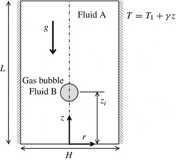
We consider the motion of an axisymmetric gas bubble of fluid ‘B’ and initial radius
 $R$
under the action of buoyancy inside a cylindrical tube of diameter
 $H$
and height
 $L$
, as shown in figure 1. The tube is filled with an incompressible, Newtonian fluid ‘A’; below, we shall take the properties of fluids A and B to reflect those of a liquid and a gas, respectively. We use cylindrical coordinates
 $(r,z)$
to model the axisymmetric bubble dynamics, starting from a position
 $z_{i}$
. Thus, the flow dynamics is assumed to be approximately symmetrical about
 $r=0$
. The rigid and impermeable wall is located at
 $r=H/2$
. The acceleration due to gravity,
 $g$
, acts in the negative
 $z$
direction, as shown in figure 1.
Schematic diagram of a bubble moving inside a Newtonian fluid under the action of buoyancy. The initial location of the bubble is at
 $z=z_{i}$
; unless specified, the values of
 $H$
,
 $L$
and
 $z_{i}$
are
 $6R$
,
 $48R$
and
 $10.5R$
, respectively. The acceleration due to gravity,
 $g$
, acts in the negative
 $z$
direction.

The equations of mass, momentum and energy conservation which govern the flow can be respectively written as:
 $$\begin{eqnarray}\displaystyle & \boldsymbol{{\rm\nabla}}\boldsymbol{\cdot }\boldsymbol{u}=0, & \displaystyle\end{eqnarray}$$
 $$\begin{eqnarray}\displaystyle & \displaystyle {\it\rho}\left[\frac{\partial \boldsymbol{u}}{\partial t}+\boldsymbol{u}\boldsymbol{\cdot }\boldsymbol{{\rm\nabla}}\boldsymbol{u}\right]=-\boldsymbol{{\rm\nabla}}p+\boldsymbol{{\rm\nabla}}\boldsymbol{\cdot }\left[{\it\mu}(\boldsymbol{{\rm\nabla}}\boldsymbol{u}+\boldsymbol{{\rm\nabla}}\boldsymbol{u}^{\text{T}})\right]+\boldsymbol{F}, & \displaystyle\end{eqnarray}$$
 $$\begin{eqnarray}\displaystyle & \displaystyle \frac{\partial T}{\partial t}+\boldsymbol{u}\boldsymbol{\cdot }\boldsymbol{{\rm\nabla}}T=\boldsymbol{{\rm\nabla}}\boldsymbol{\cdot }({\it\alpha}\boldsymbol{{\rm\nabla}}T), & \displaystyle\end{eqnarray}$$
 $\boldsymbol{u}$
,
 $p$
and
 $T$
denote the velocity, pressure and temperature fields of the fluid, respectively,
 ${\it\rho}$
and
 ${\it\mu}$
are the density and viscosity,
 $t$
represents time,
 $\boldsymbol{F}$
is the body and surface forces, such as the gravity and surface tension force per unit volume, and
 ${\it\alpha}$
denotes the thermal diffusivity. For the volume fraction,
 $c$
, which takes on values between 0 and 1 for the gaseous and liquid phases, respectively, we have the following equation:
 $$\begin{eqnarray}\frac{\partial c}{\partial t}+\boldsymbol{u}\boldsymbol{\cdot }\boldsymbol{{\rm\nabla}}c=0.\end{eqnarray}$$
In order to model the behaviour of a self-rewetting fluid, we use the following relationship for the functional dependence of the surface tension,
 ${\it\sigma}$
, on temperature:
 $$\begin{eqnarray}{\it\sigma}={\it\sigma}_{0}-{\it\beta}_{1}(T-T_{1})+{\it\beta}_{2}(T-T_{1})^{2},\end{eqnarray}$$
where
 ${\it\beta}_{1}\equiv -(\text{d}{\it\sigma}/\text{d}T)|_{T_{1}}$
and
 ${\it\beta}_{2}\equiv (\text{d}^{2}{\it\sigma}/\text{d}T^{2})/2|_{T_{1}}$
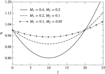
. A linear temperature variation is imposed in the vertical direction with a constant gradient
 ${\it\gamma}$
, and figure 2 shows the corresponding variation in
 ${\it\sigma}$
with
 $z$
for different values of
 ${\it\beta}_{1}$
and
 ${\it\beta}_{2}$
. As can be seen from this figure, the parabolic dependence of
 ${\it\sigma}$
on
 $z$
becomes more pronounced, with a deeper minimum, located at
 $z=z_{m}$
, for increasing
 ${\it\beta}_{1}$
and
 ${\it\beta}_{2}$
; this is expected to alter the type of Marangoni flow observed in the case of fluids that exhibit a simple linear variation of
 ${\it\sigma}$
with
 $T$
, which we will refer to in this paper as ‘linear’ fluids. Below, we will explore the dynamics of the bubble as it rises starting from
 $z_{i}$
, which may be either below or above
 $z=z_{m}$
, for both linear and self-rewetting fluids. The dependence of this dynamics on
 ${\it\beta}_{1}$
and
 ${\it\beta}_{2}$
, which parameterize the behaviour of various self-rewetting fluids, will also be studied.
Variation of the liquid–gas surface tension along the wall of the tube for
 ${\it\Gamma}=0.1$
and various values of
 $M_{1}$
and
 $M_{2}$
.

The viscosity,
 ${\it\mu}$
, is assumed to depend on the temperature and the volume fraction as follows:
 $$\begin{eqnarray}{\it\mu}=c{\it\mu}_{A}\text{e}^{-\left(T-T_{1}/T_{m}-T_{1}\right)}+(1-c){\it\mu}_{B}\left\{1+\left(\frac{T-T_{1}}{T_{m}-T_{1}}\right)^{3/2}\right\},\end{eqnarray}$$
where
 $T_{1}$
and
 $T_{m}$
are the temperatures at the bottom of the tube (
 $z=0$
) and at
 $z=z_{m}$
, respectively;
 ${\it\mu}_{A}$
and
 ${\it\mu}_{B}$
are the viscosity of the liquid and gas at temperature
 $T_{1}$
, respectively. This viscosity dependence on temperature for the liquid and gaseous phases is taken from Nahme (Reference Nahme1940). The density is given by
 $$\begin{eqnarray}{\it\rho}={\it\rho}_{A}c+{\it\rho}_{B}(1-c),\end{eqnarray}$$
while the thermal diffusivity is expressed by
 $$\begin{eqnarray}{\it\alpha}={\it\alpha}_{A}c+{\it\alpha}_{B}(1-c),\end{eqnarray}$$
in which
 ${\it\rho}_{A}$
and
 ${\it\rho}_{B}$
denote the density, while
 ${\it\alpha}_{A}$
and
 ${\it\alpha}_{B}$
represent the thermal diffusivity of the liquid and gas phases, respectively.
2.2. Scaling
The following scaling is employed to render the governing equations dimensionless:
 $$\begin{eqnarray}(r,z)=R\left(\,\widetilde{r},\widetilde{y}\,\right),\quad t=\frac{R}{V}\widetilde{t},\quad \boldsymbol{u}=V\,\widetilde{\boldsymbol{u}},\quad p={\it\rho}_{A}V^{2}\widetilde{p},\end{eqnarray}$$
 $$\begin{eqnarray}{\it\mu}={\it\mu}_{A}\widetilde{{\it\mu}},\quad {\it\rho}={\it\rho}_{A}\widetilde{{\it\rho}},\quad {\it\alpha}={\it\alpha}_{A}\widetilde{{\it\alpha}},\quad T=\widetilde{T}(T_{m}-T_{1})+T_{1},\end{eqnarray}$$
 $$\begin{eqnarray}{\it\sigma}={\it\sigma}_{0}\widetilde{{\it\sigma}},\quad {\it\beta}_{1}=\frac{{\it\sigma}_{0}}{T_{m}-T_{1}}M_{1},\quad {\it\beta}_{2}=\frac{{\it\sigma}_{0}}{(T_{m}-T_{1})^{2}}M_{2},\quad {\it\gamma}=\frac{(T_{m}-T_{1})}{R}{\it\Gamma},\end{eqnarray}$$
where the velocity scale is
 $V=\sqrt{gR}$
,
 ${\it\sigma}_{0}$
is the surface tension at
 $T_{1}$
, and the tildes designate dimensionless quantities. After dropping tildes from all non-dimensional terms, the governing dimensionless equations are given by
 $$\begin{eqnarray}\displaystyle & \boldsymbol{{\rm\nabla}}\boldsymbol{\cdot }\boldsymbol{u}=0, & \displaystyle\end{eqnarray}$$
 $$\begin{eqnarray}\displaystyle & \displaystyle \frac{\partial \boldsymbol{u}}{\partial t}+\boldsymbol{u}\boldsymbol{\cdot }\boldsymbol{{\rm\nabla}}\boldsymbol{u}=-\boldsymbol{{\rm\nabla}}p+\frac{1}{\mathit{Ga}}\boldsymbol{{\rm\nabla}}\boldsymbol{\cdot }\left[{\it\mu}(\boldsymbol{{\rm\nabla}}\boldsymbol{u}+\boldsymbol{{\rm\nabla}}\boldsymbol{u}^{\text{T}})\right]+\boldsymbol{F}, & \displaystyle\end{eqnarray}$$
 $$\begin{eqnarray}\displaystyle & \displaystyle \frac{\partial T}{\partial t}+\boldsymbol{u}\boldsymbol{\cdot }\boldsymbol{{\rm\nabla}}T=\frac{1}{\mathit{Ga}\mathit{Pr}}\boldsymbol{{\rm\nabla}}\boldsymbol{\cdot }({\it\alpha}\boldsymbol{{\rm\nabla}}T), & \displaystyle\end{eqnarray}$$
 $$\begin{eqnarray}\displaystyle & \displaystyle \frac{\partial c}{\partial t}+\boldsymbol{u}\boldsymbol{\cdot }\boldsymbol{{\rm\nabla}}c=0, & \displaystyle\end{eqnarray}$$
 $\mathit{Ga}\equiv {\it\rho}_{A}VR/{\it\mu}_{A}$
denotes the Galileo number;
 $\mathit{Pr}\equiv c_{p}{\it\mu}_{0}(T_{1})/{\it\lambda}_{A}$
is the Prandtl number, wherein
 $c_{p}$
is the specific heat capacity of the surrounding fluid and
 ${\it\lambda}_{A}$
is the thermal conductivity of the liquid. The dimensionless viscosity,
 ${\it\mu}$
, has the following dependence on
 $T$
and
 $c$
:
 $$\begin{eqnarray}{\it\mu}=c\text{e}^{-T}+(1-c){\it\mu}_{r}\left(1+T^{3/2}\right),\end{eqnarray}$$
where
 ${\it\mu}_{r}\equiv {\it\mu}_{B}/{\it\mu}_{A}$
is the viscosity ratio. The dimensionless density and thermal diffusivity are given by (Haj-Hariri et al.
Reference Haj-Hariri, Shi and Borhan1997)
 $$\begin{eqnarray}\displaystyle & {\it\rho}=c+{\it\rho}_{r}(1-c)\quad \text{and} & \displaystyle\end{eqnarray}$$
 $$\begin{eqnarray}\displaystyle & {\it\alpha}=c+{\it\alpha}_{r}(1-c), & \displaystyle\end{eqnarray}$$
 ${\it\rho}_{r}\equiv {\it\rho}_{B}/{\it\rho}_{A}$
and
 ${\it\alpha}_{r}\equiv {\it\alpha}_{B}/{\it\alpha}_{A}$
correspond to the density and thermal diffusivity ratios, respectively. In (2.13), the force
 $\boldsymbol{F}$
is given by (continuum surface force formulation Brackbill, Kothe & Zemach Reference Brackbill, Kothe and Zemach1992)
 $$\begin{eqnarray}\boldsymbol{F}=\frac{{\it\kappa}{\it\delta}_{s}}{\mathit{Bo}}\left[1-M_{1}T+M_{2}T^{2}\right]\boldsymbol{n}-{\it\rho}\boldsymbol{j},\end{eqnarray}$$
in which the first and second terms on the right-hand side correspond to the capillary and gravitational contributions, respectively. In the former, the dependence of
 ${\it\sigma}$
on
 $T$
, using (2.5), has been included. In (2.19),
 $\boldsymbol{j}$
represents the unit vector in the vertical direction,
 ${\it\kappa}$
is the curvature of the interface, calculated as the divergence of the unit normal to the interface,
 $\boldsymbol{n}$
,
 ${\it\delta}_{s}$
is the Dirac distribution function in the vicinity of the interface and
 $\mathit{Bo}\equiv {\it\rho}_{A}gR^{2}/{\it\sigma}_{0}$
is the Bond number. A discussion of the results is presented next.
3. Analytical results: Stokes flow limit
In this section, we provide a discussion of our analytical results. We derive expressions for the terminal velocity of a spherical bubble rising vertically through a quiescent and unconfined liquid in the Stokes flow limit, in which thermocapillary stresses arise due to a temperature gradient imposed on the liquid. For the purpose of this calculation we will ignore the presence of walls and consider the case of unconfined flow. We show how the dependence of the surface tension on temperature, represented by (2.5), affects the terminal bubble speed, and the magnitude and sign of the temperature gradient required to arrest bubble motion; this is also contrasted with the case of a linear fluid.
We adopt a spherically symmetric coordinate system,
 $(r,{\it\theta})$
, with the polar angle,
 ${\it\theta}$
, measured from the bottom of the bubble
 $({\it\theta}=0)$
to the top of the bubble
 $({\it\theta}={\rm\pi})$
;
 $\boldsymbol{u}=u_{r}\boldsymbol{i}_{r}+u_{{\it\theta}}\boldsymbol{i}_{{\it\theta}}$
is the velocity field, in which
 $u_{r}$
and
 $u_{{\it\theta}}$
represent its radial and azimuthal components, and
 $\boldsymbol{i}_{r}$
and
 $\boldsymbol{i}_{{\it\theta}}$
denote the unit vectors in the
 $r$
and
 ${\it\theta}$
directions, respectively. The
 $z$
-axis originates at the bubble centre and is oriented vertically upwards so that it coincides with the axis of symmetry of the bubble. The unit vector in the
 $z$
direction is expressed by
 $\boldsymbol{i}_{z}=-{\it\eta}\boldsymbol{i}_{r}+(1-{\it\eta}^{2})^{1/2}\boldsymbol{i}_{{\it\theta}}$
, in which
 ${\it\eta}\equiv \cos {\it\theta}$
. Note that we have temporarily adopted a different coordinate system from that in § 2 for the purpose of this calculation and redefined the origin of the
 $z$
-axis. At the end of the present subsection, we shall revert to the use of cylindrical coordinates. We also adopt a frame of reference that moves with the centre of the bubble, which is scaled on the steady translational speed of the bubble,
 $U$
; this speed will be determined as part of the solution. Note that all quantities presented in this subsection are in dimensional terms.
We assume that heat transfer is dominated by conduction, so that the temperature field in the liquid,
 $T$
, is governed by
 $$\begin{eqnarray}{\rm\nabla}^{2}T=0.\end{eqnarray}$$
We impose a linear temperature distribution in the liquid, so that at large distances from the bubble we have
 $$\begin{eqnarray}T_{\infty }(z)=T_{\infty }(0)+{\it\gamma}z^{\prime }.\end{eqnarray}$$
Here,
 $T_{\infty }(0)$
denotes the temperature at
 $z^{\prime }=0$
, the position of the centre of the bubble. At the bubble surface,
 $r=R$
, we demand continuity of the thermal flux:
 $$\begin{eqnarray}\frac{\partial T}{\partial r}=\left(\frac{{\it\lambda}_{B}}{{\it\lambda}_{A}}\right)\frac{\partial T_{g}}{\partial r},\end{eqnarray}$$
where
 ${\it\lambda}_{B}$
denotes the thermal conductivity of the gas and
 $T_{g}$
is the temperature of the gas bubble. We assume that
 ${\it\lambda}_{A}\gg {\it\lambda}_{B}$
, so that (3.3) reduces to
 $$\begin{eqnarray}\frac{\partial T}{\partial r}=0.\end{eqnarray}$$
The general solution of (3.1) is given by
 $$\begin{eqnarray}T=\mathop{\sum }_{n=0}^{\infty }\left[A_{n}\left(\frac{r}{R}\right)^{n}+B_{n}\left(\frac{r}{R}\right)^{-(n+1)}\right]P_{n}({\it\eta}),\end{eqnarray}$$
where
 $P_{n}({\it\eta})$
are Legendre polynomials of the first kind of degree
 $n$
, and
 $A_{n}$
and
 $B_{n}$
are coefficients. We apply the no-flux condition given by (3.4) at
 $r=R$
:
 $$\begin{eqnarray}B_{n}=\left(\frac{n}{n+1}\right)A_{n}.\end{eqnarray}$$
Substitution of (3.6) into (3.5) gives
 $$\begin{eqnarray}T=\mathop{\sum }_{n=0}^{\infty }A_{n}\left[\left(\frac{r}{R}\right)^{n}+\frac{n}{n+1}\left(\frac{r}{R}\right)^{-(n+1)}\right]P_{n}({\it\eta}).\end{eqnarray}$$
To match to the far-field condition, we set
 $z^{\prime }=r\cos ({\rm\pi}-{\it\theta})=-r\cos {\it\theta}=-r{\it\eta}$
in (3.2) so that
 $T_{\infty }(z)=T_{\infty }(0)-{\it\gamma}r{\it\eta}$
. Matching this equation to (3.7) yields
 $$\begin{eqnarray}A_{0}=T_{\infty }(0),\quad A_{1}=-{\it\gamma}R,\quad A_{n}=0\quad \text{for }n\geqslant 2.\end{eqnarray}$$
Substitution of these values into (3.7) gives
 $$\begin{eqnarray}T=T_{\infty }(0)-{\it\gamma}r\left[1+\frac{1}{2}\left(\frac{r}{R}\right)^{-3}\right]{\it\eta}.\end{eqnarray}$$
The solution for the velocity field in the fluid,
 $\boldsymbol{u}=(u_{r},u_{{\it\theta}})$
, is subject to the following boundary conditions:
 $$\begin{eqnarray}\displaystyle & \boldsymbol{u}\rightarrow -\boldsymbol{i}_{z}\quad \text{as }|\boldsymbol{r}|\rightarrow \infty , & \displaystyle\end{eqnarray}$$
 $$\begin{eqnarray}\displaystyle & u_{r}=0\quad \text{at }r=R, & \displaystyle\end{eqnarray}$$
 $$\begin{eqnarray}\displaystyle & \displaystyle {\it\tau}_{r{\it\theta}}+\frac{\partial {\it\sigma}}{\partial {\it\theta}}=0\quad \text{at }r=R, & \displaystyle\end{eqnarray}$$
 ${\it\tau}_{r{\it\theta}}$
is the tangential stress.
As noted above, the flow is axisymmetric about the
 $z$
-axis, hence the solution to the Stokes flow problem can be expressed in terms of the streamfunction,
 ${\it\psi}$
(Leal Reference Leal1992):
 $$\begin{eqnarray}{\it\psi}=UR^{2}\left[-\left(\frac{r}{R}\right)^{2}Q_{1}({\it\eta})+\mathop{\sum }_{n=1}^{\infty }\left[C_{n}\left(\frac{r}{R}\right)^{2-n}+D_{n}\left(\frac{r}{R}\right)^{-n}\right]Q_{n}({\it\eta})\right],\end{eqnarray}$$
where
 $C_{n}$
and
 $D_{n}$
are coefficients.
This is the general solution for flow past an axisymmetric body of arbitrary shape in the Stokes flow limit. Here,
 $Q_{n}$
are integrals of
 $P_{n}({\it\eta})$
, and closely related to the Gegenbauer polynomials. The polynomials relevant to the present work are
 $$\begin{eqnarray}Q_{1}({\it\eta})=\frac{1}{2}({\it\eta}^{2}-1),\quad Q_{2}({\it\eta})=\frac{{\it\eta}}{2}({\it\eta}^{2}-1).\end{eqnarray}$$
The solution expressed by (3.13) is chosen to satisfy the following equation
 $$\begin{eqnarray}E^{4}{\it\psi}=0,\end{eqnarray}$$
where
 $E^{2}$
is given by
 $$\begin{eqnarray}E^{2}\equiv \frac{\partial ^{2}}{\partial r^{2}}+\frac{(1-{\it\eta}^{2})}{r^{2}}\frac{\partial ^{2}}{\partial {\it\eta}^{2}},\end{eqnarray}$$
as well as the far-field condition given by (3.10). The streamfunction
 ${\it\psi}$
is related to
 $u_{r}$
and
 $u_{{\it\theta}}$
by
 $$\begin{eqnarray}u_{r}=-\frac{1}{r^{2}}\frac{\partial {\it\psi}}{\partial {\it\eta}},\quad u_{{\it\theta}}=-\frac{1}{r(1-{\it\eta}^{2})^{1/2}}\frac{\partial {\it\psi}}{\partial r}.\end{eqnarray}$$
It can be shown that for flow problems that have
 ${\it\psi}$
expressed as in (3.13), the component of the dimensional force along the axis of symmetry,
 $F_{z}$
, exerted by the surrounding fluid on an axisymmetric body of arbitrary shape with its centre of mass at
 $|\boldsymbol{x}|=0$
is given by the following general formula
 $$\begin{eqnarray}F_{z}=4{\rm\pi}{\it\mu}_{A}URC_{1}.\end{eqnarray}$$
At steady-state, this drag force balances the buoyancy force:
 $$\begin{eqnarray}4{\rm\pi}{\it\mu}_{A}URC_{1}={\textstyle \frac{4}{3}}{\rm\pi}({\it\rho}_{A}-{\it\rho}_{B})R^{3}g\approx {\textstyle \frac{4}{3}}{\rm\pi}{\it\rho}_{A}R^{3}g,\end{eqnarray}$$
where we have assumed that
 ${\it\rho}_{A}\gg {\it\rho}_{B}$
. Equation (3.19) suggests that
 $C_{1}$
is the only coefficient that we need to compute in order to determine the terminal velocity of the bubble.
The no-penetration condition given by (3.11) can be re-expressed as
 $\partial {\it\psi}/\partial {\it\eta}=0$
at
 $r=R$
. It follows from this condition that
 ${\it\psi}$
is constant at
 $r=R$
. Since
 ${\it\psi}=0$
at
 ${\it\theta}=0$
and
 ${\it\theta}={\rm\pi}$
, corresponding to
 ${\it\eta}=\pm 1$
, for all
 $r$
because of symmetry, then (3.11) can be rewritten as
 $$\begin{eqnarray}{\it\psi}=0\quad \text{at }r=R.\end{eqnarray}$$
Application of this condition yields
 $$\begin{eqnarray}0=-Q_{1}({\it\eta})+\mathop{\sum }_{n=1}^{\infty }\left(C_{n}+D_{n}\right)Q_{n}({\it\eta}).\end{eqnarray}$$
The tangential stress balance given by (3.12) can be re-expressed as
 $$\begin{eqnarray}-{\it\mu}_{A}r\frac{\partial }{\partial r}\left(\frac{1}{r^{2}(1-{\it\eta}^{2})^{1/2}}\frac{\partial {\it\psi}}{\partial r}\right)+\frac{\partial {\it\sigma}}{\partial {\it\theta}}=0\quad \text{at }r=R.\end{eqnarray}$$
Using (2.5), the surface tension gradient,
 $\partial {\it\sigma}/\partial {\it\theta}$
, is then given by
 $$\begin{eqnarray}\displaystyle \frac{\partial {\it\sigma}}{\partial {\it\theta}} & = & \displaystyle \frac{\partial {\it\sigma}}{\partial T}\frac{\partial T}{\partial {\it\theta}}\nonumber\\ \displaystyle & = & \displaystyle \left[-{\it\beta}_{1}+2{\it\beta}_{2}\left(T_{\infty }(0)-T_{1}-{\it\gamma}r\left[1+\frac{1}{2}\left(\frac{r}{R}\right)^{-3}\right]{\it\eta}\right)\right]\nonumber\\ \displaystyle & & \displaystyle \times \,\left({\it\gamma}r\left[1+\frac{1}{2}\left(\frac{r}{R}\right)^{-3}\right](1-{\it\eta}^{2})^{1/2}\right),\end{eqnarray}$$
where
 $T_{1}$
is a reference temperature defined in § 2.1. Substitution of (3.13) and (3.23) into (3.22) yields
 $$\begin{eqnarray}\displaystyle & & \displaystyle -2Q_{1}({\it\eta})+2C_{1}Q_{1}({\it\eta})-4D_{1}Q_{1}({\it\eta})+\mathop{\sum }_{n=2}^{\infty }\left((2-n)(1+n)C_{n}-n(n+3)D_{n}\right)Q_{n}({\it\eta})\nonumber\\ \displaystyle & & \displaystyle \quad =\frac{-3{\it\gamma}R}{2{\it\mu}_{A}U}\left(-{\it\beta}_{1}+2{\it\beta}_{2}\left[T_{\infty }(0)-T_{1}-\frac{3}{2}{\it\gamma}R{\it\eta}\right]\right)(1-{\it\eta}^{2})\nonumber\\ \displaystyle & & \displaystyle \quad =\frac{-3{\it\gamma}R{\it\beta}_{1}}{{\it\mu}_{A}U}\left[1-\frac{2{\it\beta}_{2}}{{\it\beta}_{1}}\left(T_{\infty }(0)-T_{1}\right)\right]Q_{1}({\it\eta})-\frac{9{\it\gamma}^{2}R^{2}{\it\beta}_{2}}{{\it\mu}_{A}U}Q_{2}({\it\eta}).\end{eqnarray}$$
From (3.21) we get
 $$\begin{eqnarray}-Q_{1}+(C_{1}+D_{1})Q_{1}+\mathop{\sum }_{n=2}^{\infty }\left(C_{n}+D_{n}\right)Q_{n}=0,\end{eqnarray}$$
whence
 $$\begin{eqnarray}C_{1}+D_{1}=1,\quad \text{and}\quad C_{n}=-D_{n}\quad \text{for }n\geqslant 2.\end{eqnarray}$$
For
 ${\it\beta}_{2}=0$
, i.e. for a linear fluid, then from (3.24) we get
 $$\begin{eqnarray}-2Q_{1}+2C_{1}Q_{1}-4D_{1}Q_{1}=-\frac{3{\it\gamma}R{\it\beta}_{1}}{{\it\mu}_{A}U}Q_{1},\quad \text{and}\quad C_{n}=\frac{n(n+3)}{(n+1)(2-n)}D_{n},\quad \text{for }n\geqslant 2.\end{eqnarray}$$
Thus, we deduce that
 $$\begin{eqnarray}C_{1}=1-\frac{{\it\gamma}R{\it\beta}_{1}}{2{\it\mu}_{A}U},\quad D_{1}=\frac{{\it\gamma}R{\it\beta}_{1}}{2{\it\mu}_{A}U}.\end{eqnarray}$$
For
 $n\geqslant 2$
,
 $$\begin{eqnarray}C_{n}=\frac{n(n+3)}{(n+1)(2-n)}D_{n}=-D_{n}\Rightarrow \left(\frac{n(n+3)}{(n+1)(2-n)}+1\right)D_{n}=0.\end{eqnarray}$$
However, the coefficient of
 $D_{n}$
is not zero, so
 $D_{n}=C_{n}=0$
for
 $n\geqslant 2$
. From (3.19), we arrive at the following expression for
 $U$
, after making use of
 $C_{1}$
from (3.28):
 $$\begin{eqnarray}U=\frac{{\it\rho}_{A}R^{2}g}{3{\it\mu}_{A}}\left(1+\frac{3}{2}\frac{{\it\gamma}{\it\beta}_{1}}{{\it\rho}_{A}Rg}\right).\end{eqnarray}$$
Thus, if
 $U=0$
the bubble rise is arrested provided
 $$\begin{eqnarray}{\it\gamma}={\it\gamma}_{c}=-\frac{2{\it\rho}_{A}Rg}{3{\it\beta}_{1}}.\end{eqnarray}$$
This equation implies that, for a linear fluid, the temperature gradient must be negative in order for the bubble to come to rest (Leal Reference Leal1992).
For a self-rewetting fluid with
 ${\it\beta}_{2}\neq 0$
, and following a similar procedure to that discussed above, the relevant coefficients are
 $$\begin{eqnarray}\displaystyle & \displaystyle C_{1}=1-\frac{{\it\gamma}R{\it\beta}_{1}}{2{\it\mu}_{A}U}\left[1-\frac{2{\it\beta}_{2}}{{\it\beta}_{1}}\left(T_{\infty }(0)-T_{1}\right)\right], & \displaystyle\end{eqnarray}$$
 $$\begin{eqnarray}\displaystyle & \displaystyle C_{2}=-\frac{9{\it\gamma}^{2}R^{2}{\it\beta}_{2}}{10{\it\mu}_{A}U}, & \displaystyle\end{eqnarray}$$
 $$\begin{eqnarray}\displaystyle & \displaystyle D_{1}=\frac{{\it\gamma}R{\it\beta}_{1}}{2{\it\mu}_{A}U}\left[1-\frac{2{\it\beta}_{2}}{{\it\beta}_{1}}\left(T_{\infty }(0)-T_{1}\right)\right], & \displaystyle\end{eqnarray}$$
 $$\begin{eqnarray}\displaystyle & \displaystyle D_{2}=\frac{9{\it\gamma}^{2}R^{2}{\it\beta}_{2}}{10{\it\mu}_{A}U}, & \displaystyle\end{eqnarray}$$
 $C_{n}=D_{n}=0$
for
 $n\geqslant 3$
. Substitution of
 $C_{1}$
into (3.19) yields the following expression for the terminal velocity
 $U$
:
 $$\begin{eqnarray}U=\frac{{\it\rho}_{A}R^{2}g}{3{\it\mu}_{A}}\left(1+\frac{3}{2}\frac{{\it\gamma}{\it\beta}_{1}}{{\it\rho}_{A}Rg}\left[1-\frac{2{\it\beta}_{2}}{{\it\beta}_{1}}\left(T_{\infty }(0)-T_{1}\right)\right]\right).\end{eqnarray}$$
The expression for
 ${\it\gamma}_{c}$
that leads to bubble arrest and
 $U=0$
is given by:
 $$\begin{eqnarray}{\it\gamma}_{c}=-\frac{2}{3}\frac{{\it\rho}_{A}Rg}{\displaystyle {\it\beta}_{1}\left(1-2\frac{{\it\beta}_{2}}{{\it\beta}_{1}}\left(T_{\infty }(0)-T_{1}\right)\right)}.\end{eqnarray}$$
For
 ${\it\beta}_{2}=0$
, this equation reduces to (3.31). Equation (3.37) suggests that
 ${\it\gamma}_{c}$
is positive (negative) if
 $2{\it\beta}_{2}(T_{\infty }(0)-T_{1})/{\it\beta}_{1}>1~(2{\it\beta}_{2}(T_{\infty }(0)-T_{1})/{\it\beta}_{1}<1)$
in the case of a self-rewetting fluid, in contrast to the case of a linear fluid, for which
 ${\it\gamma}_{c}<0$
.
We note that if we had assumed that the temperature distribution given by (3.2) applied everywhere, including at the bubble surface,
 $r=R$
, then the formula for the terminal velocity would have been expressed by
 $$\begin{eqnarray}U=\frac{{\it\rho}_{A}R^{2}g}{3{\it\mu}_{A}}\left(1+\frac{{\it\gamma}{\it\beta}_{1}}{{\it\rho}_{A}Rg}\left[1-\frac{2{\it\beta}_{2}}{{\it\beta}_{1}}\left(T_{\infty }(0)-T_{1}\right)\right]\right),\end{eqnarray}$$
and the expression for
 ${\it\gamma}_{c}$
by
 $$\begin{eqnarray}{\it\gamma}_{c}=-\frac{{\it\rho}_{A}Rg}{\displaystyle {\it\beta}_{1}\left(1-2\frac{{\it\beta}_{2}}{{\it\beta}_{1}}\left(T_{\infty }(0)-T_{1}\right)\right)}.\end{eqnarray}$$
Reverting back to the coordinate system of the previous section the position of the bubble centre is given by
 $$\begin{eqnarray}z=\frac{T_{\infty }(0)-T_{1}}{{\it\gamma}}\end{eqnarray}$$
and using (3.37) it is possible to derive an expression for the terminal vertical position of the bubble,
 $z_{c}$
:
 $$\begin{eqnarray}z_{c}=\left(\frac{{\it\beta}_{1}{\it\gamma}_{c}}{2}+\frac{{\it\rho}_{A}Rg}{3}\right)\frac{1}{{\it\beta}_{2}{\it\gamma}_{c}^{2}}.\end{eqnarray}$$
In the following section, we compare the predictions of (3.41) with those obtained from the numerical simulations. We turn our attention now to the numerical results.
4. Numerical results
In this section, we present a discussion of our numerical results, starting with a presentation of the numerical procedures used to carry out the computations.
4.1. Numerical method and validation
To account for the effects of inertia and confinement we solve the governing equations numerically. For the rest of the paper we will make use of the cylindrical coordinates. We use a bespoke finite-volume flow solver (Tripathi, Sahu & Govindarajan Reference Tripathi, Sahu and Govindarajan2014) that solves (2.12)–(2.14) on a staggered grid. The scalar variables (the pressure and the volume fraction of the outer fluid) are defined at the cell centres and the velocity components are defined at the cell faces, respectively. In our solver, weighted-essentially-non-oscillatory (WENO) and central difference schemes are used to discretize the advective and diffusive terms in (2.15), respectively. In order to achieve second-order accuracy, the Adams–Bashforth and Crank–Nicholson methods are used to discretize the advective and dissipation terms in (2.13), respectively.
We assume that the flow is symmetric about the axis
 $r=0$
. No-slip and no-penetration boundary conditions are used at the walls and Neumann boundary conditions are imposed at the top and bottom parts of the domain. It is to be noted that the density and the viscosity ratios in the problem considered in the present study,
 ${\it\rho}_{r}$
and
 ${\it\mu}_{r}$
, are very large, which can create spurious currents at the interface. Thus the code has been validated against Gerris, an open-source finite-volume fluid flow solver (Popinet Reference Popinet2003), which minimizes this problem by using the balanced-force continuum surface force formulation for the calculation of surface tension. We also note that in some of the cases we used only Gerris. The validation of our code is presented in figure 3, where we compare the results obtained using our code with those obtained by Sussman & Smereka (Reference Sussman and Smereka1997). Here, the parameters were chosen such that the numerical computation is particularly taxing, involving severe deformation of the bubble. The reader is also referred to the supplementary material of Tripathi et al. (Reference Tripathi, Sahu and Govindarajan2014) for an extensive validation of the present code. In addition, we have ensured that convergence is indeed achieved upon mesh refinement.
Comparison of the evolution of the shape of the bubble obtained from our simulation (shown by a solid red line) with Sussman & Smereka (Reference Sussman and Smereka1997) (dashed line) at various times in an isothermal system: (a)
 $t=0$
, (b)
 $t=0.8$
, (c)
 $t=1.6$
and (d)
 $t=2.4$
. The parameter values are
 $\mathit{Ga}=100$
,
 $\mathit{Bo}=200$
,
 ${\it\rho}_{r}=10^{-3}$
and
 ${\it\mu}_{r}=10^{-2}$
.

Below, we present a discussion of our results for the following set of ‘base’ parameters:
 $\mathit{Bo}=10^{-2}$
,
 $Ga=10$
,
 $H=6,~{\it\mu}_{r}=10^{-2}$
,
 $M_{1}=0.4$
,
 ${\it\rho}_{r}=10^{-3}$
,
 $z_{i}=10.5$
and
 ${\it\Gamma}=0.1$
, which are consistent with the case of a small air bubble rising in water due to buoyancy in the presence of strong mean surface tension, Marangoni effects and appreciable inertial contributions. We will contrast the difference in behaviour between bubble motion in linear and self-rewetting fluids by studying the effect of parameter
 $M_{2}$
on the dynamics.
4.2. Discussion
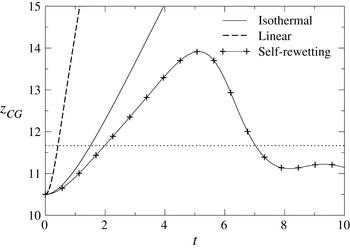
We begin the discussion of our results by showing in figure 4 the temporal variation of the centre of gravity,
 $z_{CG}$
, of a rising bubble for three different cases: the isothermal case, and the cases of a simple linear fluid and a self-rewetting fluid rising in a tube whose walls are heated with a linear temperature profile of constant gradient
 ${\it\Gamma}>0$
. It can be seen from this figure that, following an initial, relatively short, acceleration period, the bubble reaches a constant, terminal speed for both the isothermal case and the linear fluid in the non-isothermal case. The terminal velocity is higher for the non-isothermal case due to the presence of Marangoni stresses driving liquid towards the cold region of the tube and thereby enhancing the upward motion of the bubble. For the self-rewetting fluid in the non-isothermal case,
 $z_{CG}$
also reaches a constant speed for a certain time duration; this is, however, followed by a drop in
 $z_{CG}$
before a terminal
 $z_{CG}$
value is reached. Thus, the motion of a bubble rising initially in a self-rewetting fluid, whose temperature is essentially increasing linearly, is first reversed and then arrested. The fact that the bubble motion comes to a halt in the self-rewetting and not the linear fluid in a positive temperature gradient was also suggested by (3.36) in the Stokes flow limit. This property can be used to manipulate bubbles by simply shifting the temperature gradient along the wall appropriately. This might be of interest to researchers working in microfluidics and multiphase microreactors. The predictions of the dimensionless version of (3.41), given by
 $$\begin{eqnarray}z_{c}=\left(\frac{{\it\Gamma}M_{1}}{2}+\frac{\mathit{Bo}}{3}\right)\frac{1}{M_{2}{\it\Gamma}^{2}},\end{eqnarray}$$
are also shown in figure 4. For the parameters used to generate the results presented in this figure,
 $z_{c}\sim 11.67$
, which is in good agreement with the numerical predictions, despite the fact that strong inertial contributions are present in the flow, as represented by
 $Ga=10$
. We will examine the mechanism underlying this behaviour below.
Temporal variation of the centre of gravity of the bubble for the parameter values
 $\mathit{Ga}=10$
,
 $\mathit{Bo}=10^{-2}$
,
 ${\it\rho}_{r}=10^{-3}$
,
 ${\it\mu}_{r}=10^{-2}$
,
 ${\it\Gamma}=0.1$
and
 ${\it\alpha}_{r}=0.04$
. The plots for the isothermal (
 $M_{1}=0$
and
 $M_{2}=0$
), linear (
 $M_{1}=0.4$
and
 $M_{2}=0$
) and self-rewetting (
 $M_{1}=0.4$
and
 $M_{2}=0.2$
) cases are shown in the figure. The horizontal dotted line indicates the prediction of (4.1) for the self-rewetting case.

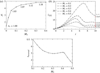
In figure 5(a), we examine the dependence of the terminal velocity
 $V_{t}$
of a bubble rising in a linear fluid on the parameter
 $M_{1}$
; the latter governs the strength of the linear variation of the surface tension with temperature. As explained above, for positive values of
 ${\it\Gamma}$
the induced Marangoni stresses increase the rise velocity of the bubble. The terminal velocity, though, appears to reach a plateau with
 $M_{1}$
, indicating that the strength of Marangoni stresses saturates at large
 $M_{1}$
. For a spherical bubble rising in an unconfined fluid, according to the analytical solution (3.30) the terminal velocity is predicted to be proportional to the parameter
 $M_{1}$
. However, in this case we consider a deformable bubble, which has a important effect on the flow. As the bubble rises, the interfacial tension decreases continuously since the bubble experiences higher temperatures. Although the value of
 $\mathit{Bo}$
evaluated at the reference temperature is rather small, indicating a relatively undeformable bubble, locally the value of
 $\mathit{Bo}$
increases, allowing the bubble to deform significantly. As indicated in figure 5(a), the aspect ratio
 $A_{r}(\equiv w/h)$
of the bubble increases (becomes more oblate) with increasing
 $M_{1}$
, which in turn increases the drag (Mahesri et al.
Reference Mahesri, Haj-Hariri and Borhan2014) resisting the upward motion of the bubble.
(a) The terminal velocity of the centre of gravity of the bubble for different values of
 $M_{1}$
for
 $M_{2}=0$
; (b) temporal variation of the centre of gravity of the bubble for
 $M_{2}=M_{1}/2$
; (c) variation of the time at which
 $z_{CG}$
reaches its maximum for different values of
 $M_{1}$
. The rest of the parameter values are
 $\mathit{Ga}=10$
,
 $\mathit{Bo}=10^{-2}$
,
 ${\it\rho}_{r}=10^{-3}$
,
 ${\it\mu}_{r}=10^{-2}$
,
 ${\it\Gamma}=0.1$
and
 ${\it\alpha}_{r}=0.04$
. The inserted numbers in (a) are the values of aspect ratio,
 $A_{r}(\equiv w/h)$
, of the bubble for different values of
 $M_{1}$
, wherein
 $h$
and
 $w$
represent the height and width of the bubble, respectively. In (b), the dotted line represents the analytical result for unbounded domain in the Stokes flow limit obtained from (3.30). The numerical predictions of (4.1) are shown by the filled square symbols on the right vertical axis of (b).

In the case of self-rewetting fluids, one parameter that we need to take into account is the position of minimum surface tension with respect to the bubble, because it will affect the action of induced Marangoni stresses; this effect will be studied in detail below. For the time being, we have positioned the centre of gravity of the bubble above the position of minimum surface tension
 $(z_{i}=10.5,z_{m}=10)$
at
 $t=0$
. In this case, as the bubble rises, it comes into contact with liquid of increasingly lower surface tension. The induced Marangoni stresses drive liquid upwards, towards the hot region of the tube, and inhibit the upward motion of the bubble. This is evident at early times in figure 4, where it is shown that the rise velocity for the self-rewetting fluid is lower than for the isothermal case.
In order to study the effect of Marangoni stress in more detail, we examine in figure 5(b) the terminal distance reached by bubbles moving in a self-rewetting fluid as a function of
 $M_{1}$
, with
 $M_{2}=M_{1}/2$
; the latter restriction is imposed in order to keep stationary the position where the minimum surface tension occurs. As shown in figure 5(b), this distance increases with decreasing
 $M_{2}$
, which indicates that an increase in the self-rewetting character of the fluid leads to a greater degree of bubble retardation: in the limit
 $M_{2}\rightarrow 0$
, a steady terminal speed is reached for
 ${\it\Gamma}>0$
. The numerical predictions for the terminal distance shown in figure 5(b) are also in good agreement with those obtained from (4.1): for the parameters used here,
 $z_{c}\sim (16.67,13.33,12.22,11.67,11.33)$
for
 $M_{1}=(0.1,0.2,0.3,0.4,0.5)$
. Also, for
 $\mathit{Bo}\sim 0$
and
 $M_{2}=M_{1}/2$
, (4.1) reduces to
 $z_{c}\sim {\it\Gamma}^{-1}$
, which for the parameters in figure 5(b) leads to
 $z_{c}\sim 10$
; this appears to be the limiting value that the terminal distance reaches with increasing
 $M_{1}$
.
Interestingly, the onset time for motion reversal,
 $t_{reversal}$
, has a non-monotonic dependence on
 $M_{1}$
: starting from a global maximum at small
 $M_{1}$
,
 $t_{reversal}$
exhibits a shallow minimum, followed by a local maximum, before undergoing a sharp decrease with increasing
 $M_{1}$
. This is probably due to the effect of inertia and the interplay between buoyancy and Marangoni stresses, which act in opposite directions. For low
 $M_{1}$
values, the Marangoni stresses are initially relatively weak and take a long time to increase enough to change the direction of motion of the bubble. As
 $M_{1}$
increases, Marangoni stresses initially become stronger, such that the bubble decelerates faster and a shorter time is needed for the motion reversal. However, as Marangoni stresses gain in relative significance, the initial acceleration of the bubble becomes considerably smaller, resulting in initially small rise velocities, therefore the bubble takes longer before it reaches the position of motion reversal. Finally, for even higher values of
 $M_{1}$
, the Marangoni stresses are so strong that they outweigh buoyancy, and the bubble very soon starts moving in the opposite direction.
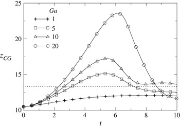
The effect of inertia on the bubble motion in a self-rewetting fluid, parameterized by the Galileo number,
 $Ga$
, is also of interest, and is shown in figure 6. As can be seen from this figure, at low values of
 $Ga$
, the bubble centre of gravity,
 $z_{CG}$
, increases monotonically with time before reaching a terminal value. Increasing the
 $Ga$
number leads to an increase in the initial rise velocity of the bubble, probably due to the fact that higher values of
 $Ga$
correspond to fluids of lower viscosity. The most interesting effect, however, is that the bubble exhibits flow reversal; the maximal
 $z_{CG}$
values reached increase progressively with
 $Ga$
prior to flow reversal, which then culminates in the bubble motion being arrested. The onset of flow reversal also appears to be an increasing function of
 $Ga$
. For the parameters used in figure 6, we find using (4.1) that
 $z_{c}\sim 13.33$
. As shown in figure 6, this value is quite close to our calculations for the terminal position of the bubble, even for high values of
 $Ga$
and in the presence of wall confinement, despite the fact that (4.1) was derived for an unconfined bubble moving in the Stokes flow limit. This is explained by the fact that at the latter stages of the flow, for all values of
 $Ga$
, the migration velocity of the bubble decreases significantly, entering into the creeping flow regime.
Effect of
 $\mathit{Ga}$
on the temporal evolution of the bubble centre of gravity for
 $\mathit{Bo}=10^{-2}$
,
 ${\it\rho}_{r}=10^{-3}$
,
 ${\it\mu}_{r}=10^{-2}$
,
 $M_{1}=0.2$
,
 $M_{2}=0.1$
,
 ${\it\Gamma}=0.1$
and
 ${\it\alpha}_{r}=0.04$
. The prediction of (4.1) is shown by the dotted line.

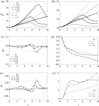
Next we examine the effect of mean surface tension, characterized by the Bond number,
 $\mathit{Bo}$
, on the bubble dynamics in a self-rewetting fluid; this is shown in figure 7(a,b) for
 $Ga=5$
and
 $Ga=10$
, respectively. It is seen clearly in figure 7(a,b) that there exists a critical value of
 $\mathit{Bo}$
above which flow reversal is no longer possible and
 $z_{CG}$
undergoes a monotonic rise with time whose rate decreases, and eventually reaches a limit with increasing
 $\mathit{Bo}$
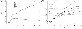
. These results highlight the role of bubble deformation in the dynamics: minimizing deformation, which is promoted by small values of
 $\mathit{Bo}$
, accelerates flow reversal, leading to lower terminal
 $z_{CG}$
values. For
 $Ga=5$
, measures of interfacial deformation are provided by the bubble length,
 $l_{B}$
, and aspect ratio of the bubble,
 $A_{r}$
, whose temporal variation are shown in figure 7(c–f), respectively, for small and large
 $\mathit{Bo}$
values. Inspection of these panels reveals that the extent of deformation increases with
 $\mathit{Bo}$
, as expected.
Effect of
 $\mathit{Bo}$
on bubble motion for (a)
 $Ga=10$
and (b)
 $Ga=5$
; effect of
 $\mathit{Bo}$
on the (c,d) length of the bubble,
 $l_{B}$
, (e,f) aspect ratio of the bubble,
 $A_{r}$
for
 $Ga=5$
. The rest of the parameter values are
 ${\it\rho}_{r}=10^{-3}$
,
 ${\it\mu}_{r}=10^{-2}$
,
 $M_{1}=0.4$
,
 $M_{2}=0.2$
,
 ${\it\Gamma}=0.1$
and
 ${\it\alpha}_{r}=0.04$
.

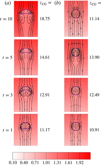
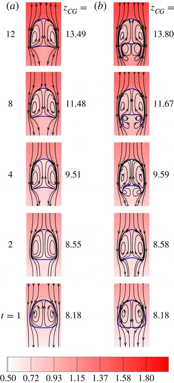
To elucidate the reasons for the behaviour depicted in figure 7, we show in figure 8 the evolution of the bubble shape and that of the temperature distribution in the fluid surrounding the bubble for two values of
 $\mathit{Bo}$
; the rest of the parameters remain fixed at their ‘base’ values. Also shown in figure 8 are streamlines which represent the structure of the flow within the bubble, in the surrounding fluid flowing past it, as well as in its wake region. It is seen that the bubble in the
 $\mathit{Bo}=10$
case (shown in figure 8
a), which rises starting from
 $z_{i}=10$
, coinciding with the surface tension minimum in figure 2, undergoes significant deformation; this begins at relatively early times, and culminates in the formation of a cap bubble. This deformation is accompanied by the formation of a pair of counter-rotating vortices within the bubble, and another pair in the wake region; the lateral and vertical extent of the latter increase with time, as the bubble rises towards the warmer regions of the tube. No evidence of flow reversal is observed, which is consistent with the results presented in figure 7.
Evolution of bubble shape (solid blue line), streamlines (lines with arrows) and temperature contours (shown in colour) with time for (a)
 $\mathit{Bo}=10$
and (b)
 $\mathit{Bo}=10^{-2}$
. The initial location of the bubble,
 $z_{i}=10$
. The inset at the bottom represents the colourmap for the temperature contours, for which values increase from bottom to top in the figures. The rest of the parameter values are
 $\mathit{Ga}=10$
,
 ${\it\rho}_{r}=10^{-3}$
,
 ${\it\mu}_{r}=10^{-2}$
,
 $M_{1}=0.4$
,
 $M_{2}=0.2$
,
 ${\it\Gamma}=0.1$
and
 ${\it\alpha}_{r}=0.04$
.

For the
 $\mathit{Bo}=10^{-2}$
case, it is seen from figure 8(b) that the bubble suffers negligible deformation, and its rise is accompanied by the formation of a pair of counter-rotating vortices inside the bubble at early times, as was also observed in the
 $\mathit{Bo}=10$
case (shown in figure 8
a). This flow structure persists until
 $t=5$
, at which the bubble is seen to develop a wake region, and two more vortices are formed within the bubble; this coincides with the onset of flow reversal, as can be ascertained upon inspection of figure 7(a). At later times, the direction of the flow is reversed, as indicated by the direction of the streamlines associated with the
 $t=10$
panel for
 $\mathit{Bo}=10^{-2}$
in figure 8(b), which points upwards since the liquid flows past a descending bubble. This is brought about by the fact that the vertical temperature gradient across the bubble is positive, which gives rise to a positive surface tension gradient since
 $z>z_{m}$
(viz. figure 2). This, then, sets up a Marangoni stress, which acts in the opposite direction to the flow past the rising bubble, retarding its motion. This stress becomes increasingly dominant, counterbalances, and then exceeds the magnitude of the buoyancy force, leading to the reversal of the bubble motion and its eventual arrest.
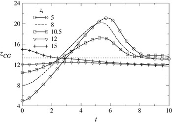
We have also studied the effect of varying the initial location of the bubble on the dynamics of the centre of gravity of bubble,
 $z_{CG}$
. In figure 9, we show the temporal evolution of
 $z_{CG}$
as a parametric function of
 $z_{i}$
, with the remaining parameters fixed at their ‘base’ values. For situations in which the initial location of the bubble is lower than that associated with the surface tension minimum in figure 2,
 $z=z_{m}$
, the surface tension gradient across the bubble reinforces the buoyancy-driven bubble rise. This results in an increase in
 $z_{CG}$
with time until the bubble reaches elevations such that
 $z>z_{m}$
, for which the sign of the surface tension gradient across the bubble is reversed, which drives Marangoni flow that acts to retard and eventually reverse the direction of bubble motion. The time associated with the onset of flow reversal decreases with increasing
 $z_{i}$
. For sufficiently large values of
 $z_{i}$
, the bubble moves in the negative
 $z$
direction under the action of Marangoni stresses whose magnitude exceeds that of the buoyancy force. The terminal value of
 $z_{CG}$
appears to be weakly dependent on
 $z_{i}$
for large
 $z_{i}$
values. Also,
 $z_{c}\sim 13.33$
from (4.1), which is in good agreement with the numerical predictions.
The effect of the initial location of the bubble on the temporal evolution of the centre of gravity,
 $z_{CG}$
. The rest of the parameter values are
 $\mathit{Ga}=10$
,
 $\mathit{Bo}=10^{-2}$
,
 ${\it\rho}_{r}=10^{-3}$
,
 ${\it\mu}_{r}=10^{-2}$
,
 $M_{1}=0.2$
,
 $M_{2}=0.1$
,
 ${\it\Gamma}=0.1$
and
 ${\it\alpha}_{r}=0.04$
. The prediction of (4.1) is shown by the dotted line.

(a) Evolution of the length of the bubble,
 $l_{B}$
, for two values of
 $\mathit{Bo}$
when the initial location of the bubble
 $z_{i}=8$
. (b) The effects of initial location of the bubble on elongation of the bubble for
 $\mathit{Bo}=100$
. The radius of the tube,
 $H=2.5$
. The rest of the parameters are
 $\mathit{Ga}=10$
,
 ${\it\rho}_{r}=10^{-3}$
,
 ${\it\mu}_{r}=10^{-2}$
,
 $M_{1}=0.4$
,
 $M_{2}=0.2$
,
 ${\it\Gamma}=0.1$
and
 ${\it\alpha}_{r}=0.04$
.

As was mentioned in the introduction, self-rewetting fluids have been used in heat pipes associated with substantially higher heat fluxes than normal liquids. In these applications, the bubbles are very confined, usually forming slugs. It therefore seems appropriate to investigate the effect of confinement. We have done this by varying the value of the dimensionless radius of the tube,
 $H$
, and plotted in figure 10(a) the temporal evolution of the bubble length,
 $l_{B}$
, for
 $\mathit{Bo}=10$
and
 $\mathit{Bo}=100$
, with
 $H=2.5$
. For this set of simulations we place the bubble below the position of minimum surface tension
 $(z_{i}=8,z_{m}=10)$
. As seen in this figure, the bubble undergoes a contraction at early times, which is followed by rapid expansion for both values of
 $\mathit{Bo}$
. This is then followed by a sustained increase (decrease) in
 $l_{B}$
with time for
 $\mathit{Bo}=100~(\mathit{Bo}=10)$
. The effect of the initial location of the bubble,
 $z_{i}$
, on the elongation of the bubble is investigated in figure 10(b). It can be seen that the length of the bubble,
 $l_{B}$
, increases as we move the initial location of the bubble in the positive
 $z$
direction.
The evolution of the bubble shape, temperature distribution and flow structure for the dynamics associated with
 $\mathit{Bo}=10$
and
 $\mathit{Bo}=100$
for parameter values the same as those used in figure 10(a) are shown in figure 11. Inspection of this figure reveals that the bubble remains essentially bullet shaped for
 $\mathit{Bo}=10$
, which is in contrast to the cap-like shape adopted by the bubble for the same
 $\mathit{Bo}$
and larger
 $H$
value. For
 $\mathit{Bo}=100$
, the bubble develops filaments in its wake region, driven by the formation of a pair of counter-rotating vortices in this region, leading to bubble elongation. This elongation is sustained by the action of the vortices whose size grows with time, causing stretching of the filaments from the main body of the bubble towards the wake region.
Evolution of bubble shape (solid blue line), streamlines (lines with arrows) and temperature contours (shown in colour) with time for (a)
 $\mathit{Bo}=10$
and (b)
 $\mathit{Bo}=100$
, and
 $H=2.5$
. The initial location of the bubble
 $z_{i}=8$
. The inset at the bottom represents the colourmap for the temperature contours, for which values increase from bottom to top in the figures. The rest of the parameters are
 $\mathit{Ga}=10$
,
 ${\it\rho}_{r}=10^{-3}$
,
 ${\it\mu}_{r}=10^{-2}$
,
 $M_{1}=0.4$
,
 $M_{2}=0.2$
,
 ${\it\Gamma}=0.1$
and
 ${\it\alpha}_{r}=0.04$
.

Next, we study the effect of the self-rewetting character of the liquid surrounding the bubble on its elongation in the presence of confinement effects. The results are shown in figure 12 for
 $\mathit{Bo}=2$
,
 $Ga=5$
, while the tube radius has been reduced to
 $H=2.1$
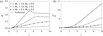
to intensify the effect of confinement; the rest of the parameters remain fixed at their ‘base’ values. It is seen clearly from figure 12(a) that the bubble elongation rate increases with
 $M_{2}(=M_{1}/2)$
; the maximal
 $l_{B}$
is reached at an earlier time with increasing
 $M_{2}$
. For the largest
 $M_{2}$
values studied, the bubble undergoes a weak contraction to an essentially terminal
 $l_{B}$
value. The bubble rise speed also increases with
 $M_{2}$
, as shown in figure 12(b), which depicts the temporal evolution of the bubble centre of gravity,
 $z_{CG}$
.
Evolution of (a) the length of the bubble,
 $l_{B}$
, (b) the location of centre of gravity, in a tube having
 $H=2.1$
. The initial location of the bubble
 $z_{i}=8$
. The rest of the parameters are
 $\mathit{Ga}=5$
,
 ${\it\rho}_{r}=10^{-3}$
,
 ${\it\mu}_{r}=10^{-2}$
. The non-isothermal curve is plotted for
 ${\it\Gamma}=0.1$
and
 ${\it\alpha}_{r}=0.04$
.

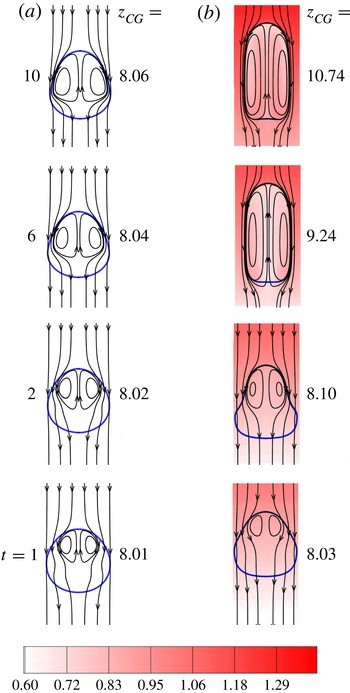
In figure 13 we contrast the flow dynamics associated with the isothermal and
 $(M_{1}=1.8,M_{2}=0.9)$
cases shown in figure 12. It is seen that, in contrast to the isothermal case, in which the bubble shape remains approximately spherical, the bubble rising in a non-isothermal, self-rewetting fluid deforms significantly in the presence of confinement, and assumes the shape of a Taylor bubble. It is difficult to compare this with the behaviour of a bubble in a linear fluid since there is no obvious basis for such a comparison.
Evolution of bubble shape (solid blue line) with time for (a) isothermal case and (b)
 $M_{1}=1.8,M_{2}=0.9$
(temperature contours shown in colour). The inset at the bottom represents the colourmap for the temperature contours, for which values increase from bottom to top in the figures. The rest of the parameters are the same as those used to generate figure 12.

5. Concluding remarks
We have carried out an analytical and numerical investigation of a gas bubble rising in a non-isothermal liquid in a cylindrical tube whose walls have a linearly increasing temperature. Two types of liquids were considered: a ‘linear’ liquid whose surface tension decreases linearly with temperature; and a so-called ‘self-rewetting’ liquid which exhibits a parabolic dependence of the surface tension on temperature, with a well-defined minimum. Attention was focused on how the latter can affect the development of thermocapillary Marangoni stresses and, in turn, the bubble dynamics.
We have shown that, in the Stokes flow limit, the motion of a spherical bubble can be arrested in a self-rewetting liquid, and derived a formula for the terminal distance in this case, even if the temperature gradient in this liquid, which surrounds the bubble, is positive. This is in contrast to the case of a linear liquid, in which a negative gradient is necessary to bring the bubble motion to a halt. We have also studied the bubble motion numerically to account for the presence of thermocapillarity, buoyancy, inertia, interfacial deformation and confinement effects. Our results have demonstrated that the motion of the bubble in a self-rewetting fluid can be reversed and then arrested in the limit of weak bubble deformation. In this limit, good agreement between the numerical and analytical predictions for the terminal distance was found, even for appreciable inertial contributions; this is due to the fact that, during the latter stages of the flow, the bubble enters the creeping flow regime prior to reaching its terminal location. The flow reversal becomes accentuated for strongly self-rewetting liquids in the presence of significant inertia. These phenomena are absent in the case of linear liquids and are attributed to the thermocapillary Marangoni stresses which oppose the direction of the buoyancy-driven bubble rise when the bubble crosses the vertical location associated with the surface tension minimum. These stresses gain in significance during the course of the flow and eventually become dominant, leading to reversal and arrest of the bubble motion.
We have also shown that a bubble in a self-rewetting fluid undergoes considerable elongation for significant confinement, forming a Taylor bubble; this is absent in the case of isothermal flows, in which the bubble remains essentially spherical.
Acknowledgements
O.K.M. wishes to thank the Engineering and Physical Sciences Research Council, UK, for their support through the MEMPHIS Programme Grant (number EP/K003976/1). K.C.S. would also like to thank Indian National Science Academy for their financial support. We thank the anonymous referee for providing an alternative derivation (included in the appendix A) of the creeping flow calculation given in § 3.
Appendix A
If we assume that convective heat transfer and drop deformation are negligible, the governing equations are linear and the motion due to gravity and thermocapillarity can be treated separately. Thus we write the drift velocity of the bubble as
 $U=U_{g}+U_{t}$
, where the gravitational contribution
 $$\begin{eqnarray}U_{g}=-\frac{{\it\rho}R^{2}}{3{\it\mu}}g.\end{eqnarray}$$
The thermocapillary contribution
 $U_{t}$
can be determined by solving the creeping flow problem.
 $$\begin{eqnarray}{\it\mu}{\rm\nabla}^{2}\boldsymbol{u}=\boldsymbol{{\rm\nabla}}p\quad \text{and}\quad \boldsymbol{{\rm\nabla}}\boldsymbol{\cdot }\boldsymbol{u}=0,\end{eqnarray}$$
 $$\begin{eqnarray}\displaystyle & \boldsymbol{n}\boldsymbol{\cdot }{\it\tau}\boldsymbol{\cdot }(\unicode[STIX]{x1D644}-\boldsymbol{n}\boldsymbol{n})=-\boldsymbol{{\rm\nabla}}_{s}{\it\sigma}\quad \text{at }r=R, & \displaystyle\end{eqnarray}$$
 $$\begin{eqnarray}\displaystyle & \boldsymbol{n}\boldsymbol{\cdot }\boldsymbol{u}=0\quad \text{at }r=R, & \displaystyle\end{eqnarray}$$
 $$\begin{eqnarray}\displaystyle & \boldsymbol{u}\rightarrow -U_{t}\boldsymbol{e}_{z}\quad \text{as }r\rightarrow \infty , & \displaystyle\end{eqnarray}$$
 ${\it\tau}=-P+(\boldsymbol{{\rm\nabla}}\boldsymbol{u}+\boldsymbol{{\rm\nabla}}\boldsymbol{u}^{\text{T}})/2$
,
 $\boldsymbol{{\rm\nabla}}_{s}$
is the surface gradient operator,
 $\boldsymbol{n}$
is the outward normal vector to the bubble surface,
 $P$
is the product of the pressure,
 $p$
, and the identity tensor,
 $\unicode[STIX]{x1D644}$
. Additionally, the drop is force-free in the thermocapillary problem, hence
 $\int _{S}{\it\tau}\boldsymbol{\cdot }\boldsymbol{n}\text{d}S=0$
, where the integral is over the bubble surface
 $S$
. Now, we invoke the Lorentz reciprocal theorem (exterior to the bubble), which states
 $$\begin{eqnarray}\int _{A}\boldsymbol{v}\boldsymbol{\cdot }{\it\tau}\boldsymbol{\cdot }\boldsymbol{n}\text{d}A+\int _{S}\boldsymbol{v}\boldsymbol{\cdot }{\it\tau}\boldsymbol{\cdot }\boldsymbol{n}\text{d}S=\int _{A}\boldsymbol{u}\boldsymbol{\cdot }{\it\Sigma}\boldsymbol{\cdot }\boldsymbol{n}\text{d}A+\int _{S}\boldsymbol{u}\boldsymbol{\cdot }{\it\Sigma}\boldsymbol{\cdot }\boldsymbol{n}\text{d}S\end{eqnarray}$$
where
 $A$
denotes an integral over a surface at infinity. In (A 6),
 $\boldsymbol{v}$
and
 ${\it\Sigma}$
are the velocity and stress fields belonging to a companion Stokes flow, which we take to be that produced by a bubble at rest in a uniform stream
 $\boldsymbol{V}$
. The first integral on the left of (A 6),
 $\int _{A}\boldsymbol{v}\boldsymbol{\cdot }{\it\tau}\boldsymbol{\cdot }\boldsymbol{n}\text{d}A=-\boldsymbol{V}\boldsymbol{\cdot }\int _{A}{\it\tau}\boldsymbol{\cdot }\boldsymbol{n}\text{d}A=0$
, since the bubble is force-free in the thermocapillary problem. The first integral on the right,
 $\int _{A}\boldsymbol{u}\boldsymbol{\cdot }{\it\Sigma}\boldsymbol{\cdot }n\text{d}A=-U_{t}\boldsymbol{e}_{z}\boldsymbol{\cdot }\int _{A}{\it\Sigma}\boldsymbol{\cdot }n\text{d}A=-4{\rm\pi}{\it\mu}R\boldsymbol{V}\boldsymbol{\cdot }(U_{t}\boldsymbol{e}_{z})$
, in which we have used the well-known result for the drag on a bubble. For the second integral on the left, note that
 $\boldsymbol{v}=(1/2)\boldsymbol{V}\boldsymbol{\cdot }(I-\boldsymbol{n}\boldsymbol{n})$
is the (purely tangential) fluid velocity at the bubble surface; hence, using the tangential stress balance in the thermocapillary problem gives
 $\int _{S}\boldsymbol{v}\boldsymbol{\cdot }{\it\tau}\boldsymbol{\cdot }\boldsymbol{n}\text{d}S=(1/2)\boldsymbol{V}\boldsymbol{\cdot }\int _{S}\boldsymbol{{\rm\nabla}}_{s}{\it\sigma}\text{d}S$
. Last, the second integral on the right of (A 6) equals zero, as there is no shear stress on the bubble in the complementary problem. Thus, we arrive at the following expression for the bubble velocity in the thermocapillary problem
 $$\begin{eqnarray}U_{t}\boldsymbol{e}_{z}=-\frac{1}{8{\rm\pi}{\it\mu}R}\int _{S}\boldsymbol{{\rm\nabla}}_{s}{\it\sigma}\text{d}S,\end{eqnarray}$$
which is essentially an average of the Marangoni stress over the bubble. Notably, (A 7) obviates the need to find the detailed flow field and is valid for any relation of surface tension to temperature.
For a self-rewetting fluid the surface tension is given by (2.5) We assume the bubble is a thermal insulator; hence, the temperature profile in the liquid
 $$\begin{eqnarray}T=T_{1}+\boldsymbol{h}\boldsymbol{\cdot }\boldsymbol{r}_{b}+\left(1+\frac{R^{3}}{2r^{3}}\right)\boldsymbol{h}\boldsymbol{\cdot }\boldsymbol{r},\end{eqnarray}$$
where
 $\boldsymbol{h}$
is the constant temperature gradient vector,
 $\boldsymbol{r}_{b}$
is the position of the bubble centre and
 $\boldsymbol{r}$
is the position vector from the centre. The difference between the temperature at the bubble centre and the reference temperature
 $T_{1}$
is equal to
 $\boldsymbol{h}\boldsymbol{\cdot }\boldsymbol{r}_{b}$
, which is equivalent to the quantity
 $T_{\infty }(0)-T_{1}$
in § 3. Inserting (A 8) into (2.5) yields
 $$\begin{eqnarray}{\it\sigma}={\it\sigma}_{0}+(-{\it\beta}_{1}+2{\it\beta}_{2}\boldsymbol{h}\boldsymbol{\cdot }\boldsymbol{r}_{b})\left(1+\frac{R^{3}}{2r^{3}}\right)\boldsymbol{h}\boldsymbol{\cdot }\boldsymbol{r}+{\it\beta}_{2}(\boldsymbol{h}\boldsymbol{\cdot }\boldsymbol{r}_{b})^{2}+{\it\beta}_{2}\left(1+\frac{R^{3}}{2r^{3}}\right)^{2}(\boldsymbol{h}\boldsymbol{\cdot }\boldsymbol{r})^{2}.\end{eqnarray}$$
The first and third terms in the above are constant and, therefore, do not generate a Marangoni stress. The fourth term generates a Marangoni stress that is symmetric about the bubble centre, due to the quadratic dependence of the surface tension on
 ${\it\beta}_{2}$
. This symmetry dictates that the fourth term does not yield a contribution to the thermocapillary velocity of the bubble. However, the second term does drive a Marangoni stress that contributes to the bubble velocity; specifically, from (A 9)
 $$\begin{eqnarray}\boldsymbol{{\rm\nabla}}_{s}{\it\sigma}={\textstyle \frac{3}{2}}(-{\it\beta}_{1}+2{\it\beta}_{2}\boldsymbol{h}\boldsymbol{\cdot }\boldsymbol{r}_{b})\boldsymbol{h}\boldsymbol{\cdot }(I-nn)+\cdots \,,\end{eqnarray}$$
where
 $\cdots \!$
indicates the Marangoni stress from the fourth term in (A 9), which, as mentioned above, does not contribute to the bubble velocity. Inserting (A 10) into (A 7) and performing the required integration yields
 $$\begin{eqnarray}U_{t}=\frac{{\it\beta}_{1}R}{2{\it\mu}}\left(1-\frac{2{\it\beta}_{2}}{{\it\beta}_{1}}\boldsymbol{h}\boldsymbol{\cdot }\boldsymbol{r}_{b}\right),\end{eqnarray}$$
which when summed with the gravitational velocity (A 1) yields the total bubble velocity given in (3.36). This derivation was provided by the anonymous referee.