





1. Introduction
The remarkable efficiency of insect and bird flight has inspired a plethora of recent studies investigating propulsion by both rigid and flexible flapping plates (Pullin & Wang Reference Pullin and Wang2004; Hua et al. Reference Hua, Zhu and Lu2013; Huang et al. Reference Huang, Nitsche and Kanso2016; Liu et al. Reference Liu, Huang and Lu2020; Alben Reference Alben2021a
,
Reference Albenb
; Nitsche et al. Reference Nitsche, Oza and Siegel2025). These studies are motivated in part by their implications for the control and design of bio-inspired robots and micro air vehicles. In the same spirit, many authors have employed computational and experimental techniques to study the aerodynamic forces experienced by plates undergoing highly unsteady aerial manoeuvres such as a complex pitch–ramp motion (Eldredge et al. Reference Eldredge, Wang and Ol2009; Ol et al. Reference Ol, Eldredge and Wang2009; Yu et al. Reference Yu, Amandolese, Fan and Liu2018). The relevant Reynolds numbers (
 ${\textit{Re}}$
) of such manoeuvres are typically
 ${\sim}10^2$
–
 $10^4$
(Eldredge et al. Reference Eldredge, Wang and Ol2009). Exploring large parameter spaces at these Reynolds numbers quickly becomes computationally prohibitive. As a result, many authors have turned to inviscid vortex sheet models as a computationally efficient alternative that can model and explain the aerodynamic mechanisms behind force generation during these manoeuvres (Alben et al. Reference Alben, Witt, Baker, Anderson and Lauder2012; Ramesh et al. Reference Ramesh, Gopalarathnam, Granlund, Ol and Edwards2014; Huang et al. Reference Huang, Nitsche and Kanso2016). The physics of force generation on a body can often be explained by relating the unsteady forces to the vortex shedding patterns induced by the body (Alben Reference Alben2021a
). Hence, by distilling the entire fluid–body system into a simplified vortex structure, vortex sheet models offer a promising route to both explaining and accurately predicting the aerodynamic forces experienced by plates and foils in terms of their vortex shedding patterns.
Several studies have compared inviscid vortex sheet models with direct Navier–Stokes simulations and/or experiments, in terms of the forces and vortex structures induced by solid bodies in flows (Nitsche & Krasny Reference Nitsche and Krasny1994; Knowles et al. Reference Knowles, Wilkins, Ansari and Zbikowski2007; Pan et al. Reference Pan, Dong, Zhu and Yue2012; Sheng et al. Reference Sheng, Ysasi, Kolomenskiy, Kanso, Nitsche and Schneider2012; Xia & Mohseni Reference Xia and Mohseni2013; Ramesh et al. Reference Ramesh, Gopalarathnam, Granlund, Ol and Edwards2014; Darakananda et al. Reference Darakananda, Eldredge, Colonius and Williams2016; Faure et al. Reference Faure, Dumas, Drouet and Montagnier2019). In Pan et al. (Reference Pan, Dong, Zhu and Yue2012), excellent agreement was obtained between the time-averaged thrust forces measured for a flapping airfoil in experiment and an inviscid vortex sheet model. A key caveat, however, is that good agreement was found only when leading-edge vortex shedding was included in the inviscid model. In both Pan et al. (Reference Pan, Dong, Zhu and Yue2012) and Sheng et al. (Reference Sheng, Ysasi, Kolomenskiy, Kanso, Nitsche and Schneider2012), omitting leading-edge shedding from the inviscid model led to relatively poor agreement with the forces computed by a direct Navier–Stokes simulation.
These observations motivate a closer examination of leading-edge vortex shedding in vortex sheet simulations, which remains a central difficulty for such models. When leading-edge shedding occurs, free vorticity released from the body often remains very close to the body surface; by contrast, vorticity released at the trailing edge is quickly advected away. As a result, computing the velocity of vorticity released at the leading edge often involves a so-called ‘near-singular integral’, which can introduce severe numerical error (Nitsche Reference Nitsche2021) that persists in the inviscid setting due to the absence of viscous dissipation. Aside from these numerical issues, there is also a physical ambiguity. In inviscid flow, the boundary condition enforces no-penetration but not no-slip, so newly shed vorticity must leave the body tangent to its edges. Hence, when the flow at a plate edge is directed onto the edge, it may not be clear to which side of the plate newly shed vortex particles should be advected.
Many vortex sheet models therefore deliberately halt the shedding of vorticity at the leading edge when the flow is directed onto it (Alben Reference Alben2010a
; Huang et al. Reference Huang, Nitsche and Kanso2016; Sohn Reference Sohn2024; Nitsche et al. Reference Nitsche, Oza and Siegel2025). This is done especially frequently in coupled simulations, where the motion of the body is driven by the fluid forces and can become unstable in the presence of leading-edge shedding. When the motion of the body is prescribed (i.e. not coupled to the fluid forces), there is a related body of work surrounding the so-called ‘leading-edge suction parameter’ (LESP): an experimentally determined quantity used in vortex sheet simulations to determine when leading-edge shedding should occur for bodies with rounded edges (Ramesh et al. Reference Ramesh, Gopalarathnam, Granlund, Ol and Edwards2012, Reference Ramesh, Gopalarathnam, Granlund, Ol and Edwards2014; Narsipur et al. Reference Narsipur, Ramesh, Gopalarathnam and Edwards2023). This parameter depends on both the prescribed motion and the geometry of the body, and can be viewed as a modelling choice that allows one to fit vortex sheet simulations to experiments or direct Navier–Stokes simulations. In Faure et al. (Reference Faure, Dumas, Drouet and Montagnier2019), for example, the critical LESP value was chosen based on the body geometry and the desired
 ${\textit{Re}}$
. In practice, both special quadrature rules (Nitsche Reference Nitsche2021; Sohn Reference Sohn2024) and smoothing techniques (Alben Reference Alben2010b
; Alben et al. Reference Alben, Miller and Peng2013) are often necessary to resolve the near-leading-edge flow accurately and robustly in vortex sheet models.
Recently, a vortex sheet model has been proposed by the present authors that allows for stable, continuous leading-edge vortex shedding in vortex sheet simulations with strong flow-body coupling (Loo & Alben Reference Loo and Alben2025). This model was used to simulate freely falling plates undergoing both side-to-side fluttering and end-over-end tumbling. Its predicted value of the plate density parameter where fluttering transitions to tumbling was consistent with both experiments and direct Navier–Stokes simulation (Loo & Alben Reference Loo and Alben2025). Here, we build on that approach with an improved formulation and address a complementary but distinct question: to what extent can an inviscid vortex sheet model with continuous leading-edge shedding quantitatively reproduce forces and vortex dynamics from direct Navier–Stokes simulations?
Previous comparisons between vortex sheet models and viscous simulations have typically focused on a small number of representative kinematics, chosen to illustrate specific flow features or the capabilities of a given formulation. These studies have played an important role in establishing the physical relevance of inviscid formulations. At the same time, because treatments of leading-edge shedding were often sensitive to kinematics or relied on model-specific assumptions, extending such comparisons in a uniform way across a broad range of unsteady motions has remained challenging. The continuous leading-edge shedding framework introduced in Loo & Alben (Reference Loo and Alben2025) reduces these sensitivities and allows us to conduct a more systematic assessment. In the present study, we use a single vortex sheet model to compare force predictions with direct Navier–Stokes simulations for
 ${\approx} 70$
distinct plate manoeuvres, providing a broad evaluation of model performance across a wide range of conditions.
A meaningful comparison requires that the viscous simulations accurately represent the same zero-thickness geometry assumed by the vortex sheet model. Indeed, the flows induced by plates of zero and small but non-zero thickness can be quite different. In Nuriev et al. (Reference Nuriev, Kamalutdinov and Egorov2019), for instance, the relative error between the time-averaged pressure drag on an oscillating plate with zero and non-zero thickness (
 $5\,\%$
of the plate length) at
 ${\textit{Re}} = 1000$
is as large as
 ${\approx} 15\,\%$
. The pressure jump across a zero-thickness plate is greater at all times, consistent with the classical result that the normal force on the plate increases with decreasing thickness in an unbounded domain (Plotkin & Kennell Reference Plotkin and Kennell1981). A similar effect arises when the leading edge of a flat plate is rounded, which can change the normal force coefficient by about
 $25\,\%$
, possibly by altering both the separation point and circulation intensity at the leading edge (Rival et al. Reference Rival, Kriegseis, Schaub, Widmann and Tropea2014). In many of the aforementioned studies comparing inviscid models with direct Navier–Stokes simulations, the zero-thickness plate is instead approximated by a plate of small but non-zero thickness (
 ${\approx} 2$
–
 $6\,\%$
of the plate length).
At the same time, accurate Navier–Stokes simulation of a plate of exactly zero thickness presents well-known numerical challenges. The pressure and vorticity fields exhibit inverse-square-root singularities at the plate tips (Koumoutsakos & Shiels Reference Koumoutsakos and Shiels1996; Alben Reference Alben2021a ), and resolving these requires specialised numerical treatment. Prior studies have addressed these difficulties using approaches such as grid clustering near the tips (Tamaddon-Jahromi et al. Reference Tamaddon-Jahromi, Townsend and Webster1994; Najjar & Vanka Reference Najjar and Vanka1995; Alben Reference Alben2021a ), viscous particle methods that integrate vorticity to remove singular behaviour (Koumoutsakos & Shiels Reference Koumoutsakos and Shiels1996) and discrete kernel methods suitable for high-Reynolds-number immersed-plate problems (Sader et al. Reference Sader, Hou, Hinton, Pullin and Colonius2024). Even with high-order methods and fine resolution, the computed forces can differ significantly depending on how the singular region is treated (Najjar & Vanka Reference Najjar and Vanka1995; Xu & Nitsche Reference Xu and Nitsche2014). Following Alben (Reference Alben2021a ), Tamaddon-Jahromi et al. (Reference Tamaddon-Jahromi, Townsend and Webster1994), Najjar & Vanka (Reference Najjar and Vanka1995), we therefore cluster the grid near the plate tips to mitigate these singularities.
In this study, we consider plates of exactly zero thickness and validate our viscous solver against the benchmark results of Koumoutsakos & Shiels (Reference Koumoutsakos and Shiels1996). We then compare the aerodynamic forces and resulting vorticity fields for several unsteady plate manoeuvres using both direct Navier–Stokes simulations and an improved vortex sheet model with continuous leading-edge shedding. This comparison will help elucidate which vortex-dynamical features of unsteady high-Re flows can be approximated well by inviscid models. Because inviscid vortex sheet simulations are both orders of magnitude faster and less expensive than corresponding viscous simulations, the present results also indicate where such models can be reliably used for rapid exploration of large kinematic parameter spaces or control.
The structure of the paper is as follows. In § 2 we describe our viscous (§ 2.1) and inviscid (§ 2.2) models. Section 3 compares the forces and induced vorticity fields in five scenarios, namely plate oscillation (§ 3.1), heaving and pitching (§ 3.2), pitch-up (§ 3.3), uniform rotation (§ 3.4) and steady translation (§ 3.5). In § 4 we summarise our findings and conclude in § 5.
2. Methodology and validation
Here we describe both the viscous and inviscid numerical models of the zero-thickness plate. In both models, we assume two-dimensional flow, and the plate is represented by a line segment of unit length. The motion of the plate is completely characterised by two quantities, the position of its centre of mass and its orientation angle (i.e. the oriented angle a line tangent to the plate makes with the
 $x$
-axis) denoted by
 \begin{align} \boldsymbol{X}_G(t) &: \text{plate centre of mass} \nonumber \\ \beta (t) &: \text{plate orientation angle} \end{align}
2.1. Viscous numerical model
We consider a plate with zero thickness and unit length occupying the interval
 $[-1/2,1/2]$
on the
 $x$
-axis and solve the two-dimensional Navier–Stokes equations in the body frame of the plate (Li et al. Reference Li, Sherwin and Bearman2002) given by
 \begin{equation} \begin{cases} \partial _t \boldsymbol{u} + \boldsymbol{u}\boldsymbol{\cdot }\boldsymbol{\nabla }\boldsymbol{u} - \dfrac {1}{{\textit{Re}}}\Delta \boldsymbol{u} = -\boldsymbol{\nabla }\!p - 2\boldsymbol{\varOmega }\times \boldsymbol{u} - \boldsymbol{\varOmega }\times (\boldsymbol{\varOmega }\times \boldsymbol{r}) -\dot {\boldsymbol{\varOmega }}\times \boldsymbol{r} - \boldsymbol{A}(t) \\[5pt] \boldsymbol{\nabla }\boldsymbol{\cdot }\boldsymbol{u} = 0 \end{cases} \end{equation}
A complete derivation of (2.2) is given in Appendix A. Here,
 $\boldsymbol{r} = [x,y,0]^T$
,
 $\boldsymbol{u} = [u,v,0]^T$
is the fluid velocity,
 $\boldsymbol{A}(t) = [A_x(t),A_y(t),0]^T$
is the acceleration of the plate centre of mass (expressed in body-frame coordinates),
 $\boldsymbol{\varOmega }(t) = [0,\ 0,\ \varOmega (t)]^T$
is the vector of angular velocity of the plate about its centre of mass and
 $\dot {\boldsymbol{\varOmega }}(t)=[0,\ 0,\ \dot \varOmega (t)]^T$
is its angular acceleration vector. By definition, we have that
 $({\rm d}/{\rm d}t)\beta (t) = \varOmega (t)$
. We non-dimensionalise distances by the plate length
 $L$
and velocities by a characteristic velocity
 $U$
defined separately for each problem in § 3. Then
 ${\textit{Re}} = UL/\nu$
is a dimensionless inverse viscosity that we set to 1000. These equations can be simplified in terms of the variables
 $u,v,p$
yielding
 \begin{equation} \begin{cases} \partial _t u + u\partial _xu + v\partial _yu - \dfrac {1}{{\textit{Re}}}\Delta u= -\partial _x p + 2\varOmega v + \dot {\varOmega }y +\varOmega ^2x - A_x,\\[7pt] \partial _t v + u\partial _xv + v\partial _yv - \dfrac {1}{{\textit{Re}}}\Delta v= -\partial _y p -2\varOmega u - \dot {\varOmega }x + \varOmega ^2y - A_y, \\[5pt] \partial _x u + \partial _y v = 0. \end{cases} \end{equation}
Henceforth we let
 $\boldsymbol{r} = [x,y]^T$
,
 $\boldsymbol{u} = [u,v]^T$
and
 $\boldsymbol{A}(t) = [A_x(t),A_y(t)]^T$
. Since the centrifugal force
 $[\varOmega (t)^2x,\varOmega (t)^2 y]^T$
and the inertial force
 $[-A_x(t),-A_y(t)]^T$
are conservative, we may write them as the gradient of a potential:
 \begin{equation} [\varOmega (t)^2x - A_x(t),\varOmega (t)^2y - A_y(t)]^T = \boldsymbol{\nabla }\left(\frac {1}{2}\varOmega (t)^2 (x^2 + y^2)- A_x(t)x - A_y(t)y \right)\!. \end{equation}
Hence, as the pressure is unique only up to the addition of a potential, we may absorb these forces into the pressure to form the simplified equations:
 \begin{equation} \begin{cases} \partial _t u + u\partial _xu + v\partial _yu - \dfrac {1}{{\textit{Re}}}\Delta u= -\partial _x p + 2\varOmega v + \dot {\varOmega }y,\\[9pt] \partial _t v + u\partial _xv + v\partial _yv - \dfrac {1}{{\textit{Re}}}\Delta v= -\partial _y p -2\varOmega u - \dot {\varOmega }x, \\[5pt] \partial _x u + \partial _y v = 0. \end{cases} \end{equation}
Note that only the Coriolis force
 $[2\varOmega v,-2\varOmega u]^T$
and the Euler force
 $[\dot \varOmega y,-\dot \varOmega x]^T$
remain, as these forces are non-conservative.
Having presented the equations, we now briefly describe how we solve them numerically. Our viscous model for the flat plate is based on the method described in Alben (Reference Alben2021a
) with a few modifications. A similar model was also employed to study heat transfer from a flapping plate in Wang & Alben (Reference Wang and Alben2025) and validated at
 $ {\textit{Re}}\sim 150$
. Here we briefly review some of the essential details. The system of (2.5) is solved on a rectangular grid with length
 $\ell _x$
and width
 $\ell _y$
in the
 $x$
and
 $y$
directions, respectively. Here
 $x$
and
 $y$
are discretised with
 $m$
and
 $n$
points, respectively. It is a finite-difference method, using a second-order stencil to compute spatial derivatives on a staggered marker-and-cell (MAC) grid aligned with the plate. The grid is non-uniform, and clustered near both the sides and edges of the plate. More precisely, assume we have (piecewise) uniformly spaced grids on
 $X$
and
 $Y$
such that
 \begin{align} -l_x/2 \lt X \lt l_x/2,\ -l_y/2 \lt Y \lt l_y/2. \end{align}
Here
 $l_x$
and
 $l_y$
are the length and width, respectively, of the computational domain. The uniform grids are mapped to non-uniform grids on
 $(x, y)$
by
 \begin{equation} x = \begin{cases} X - \eta _L\dfrac {l_x - 1}{4\pi }\sin (4\pi (X - 1/2)/(l_x - 1)), & \text{if } -l_x/2 \lt X \lt -1/2 ,\\[11pt] X + \eta \dfrac {1}{2\pi }\sin (2\pi X), & \text{if } -1/2 \lt X \lt 1/2, \\[11pt] X - \eta _R \dfrac {l_x - 1}{4\pi }\sin (4\pi (X + 1/2)/(l_x- 1)), & \text{if } 1/2\lt X \lt l_x/2 ,\end{cases} \end{equation}
 \begin{equation} y = Y + \eta \frac {l_y}{2\pi }\sin \left(\frac {2\pi }{l_y} Y \right)\!. \end{equation}
Here we take
 $l_y = l_x = 22$
and
 $\eta = 0.95$
. We choose
 $\eta _L$
and
 $\eta _R$
so that the mesh length changes smoothly across the edges of the plate (i.e. the mesh length is a smooth function of
 $x$
at
 $\pm 1/2$
). Concentrating the grid points near the edges of the plate is necessary to suppress the inverse-square-root singularities in both the vorticity and pressure fields and allow for accurate computation of aerodynamic forces. As discussed in (Alben Reference Alben2021a
), these singularities can also pose an obstruction to convergence. The highly stretched grid does however raise the condition number of the linear system (Alben Reference Alben2021a
). Since the Navier–Stokes equations are solved in the body frame of the plate, the
 $x$
-axis of the grid is aligned with the plate regardless of its orientation angle.
In all that follows,
 $X$
and
 $Y$
are discretised with
 $768$
points. The minimum and maximum mesh lengths are roughly
 $4\times 10^{-4}$
and
 $6\times 10^{-2}$
, respectively. We choose
 ${\rm d}t = 2\times 10^{-4}$
so that for each motion and corresponding characteristic velocity
 $U$
the maximum convective CFL number
 $\approx ( {{\rm d}t}/{\min {{\rm d}x}})U \leq 0.5 \lt 1$
. The time derivative is discretised with second-order backward differentiation (BDF2) and we solve for the pressure iteratively using a variation of the SIMPLE scheme (Ferziger et al. Reference Ferziger, Perić and Street2019). To accelerate convergence we apply a sixth-order Shapiro filter (Falissard Reference Falissard2013) before solving for the pressure at each iteration of the SIMPLE scheme.
2.1.1. Boundary conditions
We seek to solve (2.5) on an unbounded domain. Assuming that the plate is initially at rest, the motion of the plate is completely determined by the translational velocity of the plate centre of mass
 $\boldsymbol{U}(t)$
and its angular velocity
 $\varOmega (t)$
. To be precise, the translational velocity expressed in body-frame coordinates,
 $\boldsymbol{U}(t)$
, is given by
 \begin{equation} \boldsymbol{U}(t) = R_{-\beta (t)} \frac {\rm d}{{\rm d}t}\boldsymbol{X}_G(t). \end{equation}
The vector
 $( {\rm d}/{{\rm d}t})\boldsymbol{X}_G(t)$
gives the translational velocity of the plate centre in the laboratory frame. The rotation
 $R_{-\beta (t)}$
changes coordinates, expressing this velocity in the body frame. We illustrate this in figure 1. In panel (a) we show an example of the plate in the lab frame, at position
 $\boldsymbol{X}_G(t) = [X_G(t),Y_G(t)]^T$
making orientation angle
 $\beta (t)$
with the
 $x$
-axis and moving in the direction
 $({\rm d}/{{\rm d}t})\boldsymbol{X}_G(t)$
. In panel (b) we show the corresponding situation in the body frame. The plate occupies
 $[-1/2,1/2]\times \{0\}$
and the velocity of the body expressed in the coordinates of the body frame must be rotated so that
 $\boldsymbol{U}(t) = R_{-\beta (t)}({\rm d}/{{\rm d}t})\boldsymbol{X}_G(t)$
.
Schematic showing the plate in
 $(a)$
the lab frame and
 $(b)$
the body frame.

The reason for this definition is that for a plate moving with velocity
 $({\rm d}/{{\rm d}t})\boldsymbol{X}_G(t)$
, in the body frame of the plate, the far field moves with velocity
 \begin{equation} \boldsymbol{U}_{\!f}(t,x,y) = [U_{\!f}(t,x,y),V_{\!f}(t,x,y)]^T =-\boldsymbol{U}(t) - [-\varOmega (t) y, \varOmega (t) x]^T. \end{equation}
Let
 $\hat {\boldsymbol{S}}$
and
 $\hat {\boldsymbol{N}}$
denote the unit tangent vector and inward unit normal vector, respectively, along the computational boundary (with anticlockwise orientation). We use the far-field velocity
 $\boldsymbol{U}_{\!f}$
to impose Dirichlet and Neumann boundary conditions on the boundary where
 $\boldsymbol{U}_{\!f}$
is flowing into and out of the fluid domain, respectively. The tangential velocity at the boundary is specified with Neumann boundary conditions. Stated more precisely, for each point in our computational boundary, we let
 \begin{align} \begin{cases} \partial _{\hat {\boldsymbol{N}}}(\boldsymbol{u}-\boldsymbol{U}_{\!f} ) = 0\ &\text{ if } \boldsymbol{U}_{\!f}\boldsymbol{\cdot }\hat {\boldsymbol{N}} \lt 0, \\[7pt] \partial _{\hat {\boldsymbol{N}}}(\boldsymbol{u} - \boldsymbol{U}_{\!f})\boldsymbol{\cdot }\hat {\boldsymbol{S}} = 0,\ (\boldsymbol{u} - \boldsymbol{U}_{\!f})\boldsymbol{\cdot }\hat {\boldsymbol{N}}=0\ &\text{ if } \boldsymbol{U}_{\!f}\boldsymbol{\cdot }\hat {\boldsymbol{N}} \gt 0. \end{cases} \end{align}
To suppress any spurious vorticity that may be generated at the walls of the computational domain, we supplement our boundary conditions with an absorbing sponge layer using Rayleigh damping near the computational boundaries (Slinn & Riley Reference Slinn and Riley1998). This approach has been used successfully to suppress boundary reflections in both incompressible (Slinn & Riley Reference Slinn and Riley1998; Pant & Bhattacharya Reference Pant and Bhattacharya2016) and compressible (Hu Reference Hu2005; Hu et al. Reference Hu, Li and Lin2008) vortex-dominated flows in an unbounded domain. The application of this sponge boundary condition consists of adding a damping term
 \begin{equation} -\sigma (x,y)(\boldsymbol{u} -\boldsymbol{U}_{\!f}) \end{equation}
to the right-hand side of (2.5) in a thin region (sponge layer) containing the boundary. Here we take the damping function to be
 \begin{equation} \sigma (x,y) = \begin{cases} 0.5((x^2 + y^2)^{ 1/2}-R)^{3} & \text{if } x^2 +y^2 \gt R^2, \\[5pt] 0 & \text{otherwise.} \end{cases} \end{equation}
Here
 $\sigma (x,y)$
controls the strength and spatial distribution of the absorbing layer (Hu et al. Reference Hu, Li and Lin2008), where
 $R=8$
defines the radius of our computational domain, so that our sponge layer has a minimum thickness of
 $\epsilon = 3$
. Note that outside this circle, the true Navier–Stokes equations are not being solved, and hence we think of the region outside the circle as part of the boundary, not the computational domain.
2.1.2. Validation
To validate our viscous solver, we consider an impulsively started flat plate moving normal to itself with unit speed at
 ${\textit{Re}} = 1000$
. In figure 2 we compare the computed forces between our viscous solver with the numerical results of Koumoutsakos & Shiels (Reference Koumoutsakos and Shiels1996). The results are in good agreement.
(a) The drag coefficient
 $F_D$
and (b) the length of the recirculation bubble
 $S$
over time for an impulsively started flat plate moving normal to itself with unit speed at
 ${\textit{Re}} = 1000$
, compared with data obtained from figure 13 in Koumoutsakos & Shiels (Reference Koumoutsakos and Shiels1996).

In figure 3 we reproduce the vorticity contours shown in figure 20 of Koumoutsakos & Shiels (Reference Koumoutsakos and Shiels1996). The circulation bubble is outlined in black, and our vorticity is presented on a bi-directional logarithmic scale, with contour levels ranging from
 $\pm 2^{-4}$
to
 $\pm 2^{10}$
. Here, the vorticity contours are visualised with the perceptually uniform colour map ‘balance’ described in Thyng et al. (Reference Thyng, Greene, Hetland, Zimmerle and DiMarco2016) (i.e. each doubling of vorticity magnitude corresponds to a fixed decrease in colour brightness). Each panel is overlaid with the corresponding streamlines (top half) and vorticity contours (bottom half) in figure 20 in Koumoutsakos & Shiels (Reference Koumoutsakos and Shiels1996). In the top half of each panel the streamlines from Koumoutsakos & Shiels (Reference Koumoutsakos and Shiels1996) inside are given as dotted lines, while in the bottom half of each panel, the vorticity contours are given as dark lines. The circulation bubble in the top half of the figure in Koumoutsakos & Shiels (Reference Koumoutsakos and Shiels1996) overlaps with the present viscous model.
Vorticity fields (labelled by colour bar) for an impulsively started plate at times
 $t$
= 0.5, 2.5, 6 and 10, with circulation bubble outlined in black and
 ${\textit{Re}} = 1000$
. The streamlines (a,b) and vorticity contours (c,d) from figure 20 in Koumoutsakos & Shiels (Reference Koumoutsakos and Shiels1996) are overlaid on each panel.

Figure 3. Long description
Panel A: A contour plot shows the vorticity field for an impulsively started plate at time t = 0.5. The x-axis ranges from −1.5 to 1.5 and the y-axis ranges from 0 to 3. The circulation bubble is outlined in black. The top half of the panel displays streamlines, while the bottom half shows vorticity contours overlaid on the vorticity field. Panel B: A contour plot shows the vorticity field for an impulsively started plate at time t = 2.5. The x-axis ranges from −1.5 to 1.5 and the y-axis ranges from 0 to 3. The circulation bubble is outlined in black. The top half of the panel displays streamlines, while the bottom half shows vorticity contours overlaid on the vorticity field. Panel C: A contour plot shows the vorticity field for an impulsively started plate at time t = 6. The x-axis ranges from -1.5 to 1.5 and the y-axis ranges from 0 to 3. The circulation bubble is outlined in black. The top half of the panel displays streamlines, while the bottom half shows vorticity contours overlaid on the vorticity field. Panel D: A contour plot shows the vorticity field for an impulsively started plate at time t = 2.5. The x-axis ranges from -1.5 to 1.5 and the y-axis ranges from 0 to 3. The circulation bubble is outlined in black. The top half of the panel displays streamlines, while the bottom half shows vorticity contours overlaid on the vorticity field.
In figure 4 we show a grid refinement study using the drag coefficient
 $F_D$
of this example of an impulsively started plate moving normal to itself. We consider grid sizes
 $n = m = 256, 384, 576, 864, 1296$
, the grid sizes increasing by factors of
 $3/2$
. We plot the relative
 $L^2$
error against the number of grid points
 $n = m$
with a log–log scale. The relative
 $L^2$
error of the drag force
 $F_D$
is given by
 \begin{equation} L^2\textrm { error} = \frac {\|F_D(t) - F_D^{\textit{ref}}(t)\|_{L^2}}{\|F_D^{\textit{ref}}(t)\|_{L^2}}, \end{equation}
where the reference drag coefficient
 $F_D^{\textit{ref}}$
is obtained by Richardson extrapolation from the solutions on the two finest grids (
 $n = m = 864, 1296$
). As shown by the dotted line in figure 4, the four points are approximately collinear with the dotted line with slope
 $-2$
. Hence, we see that the
 $L^2$
error is approximately second order with respect to the number of grid points, which is consistent with the numerical scheme described in § 2.1. As discussed in § 2.1, we take
 $n = m = 768$
in this study, where the relative
 $L^2$
error of the forces is
 ${\lessapprox} 0.2\,\%$
.
Relative
 $L^2$
error against number of grid points in each axis
 $n$
. The dotted line has slope
 $-2$
and passes through the first data point.

2.2. Inviscid numerical model
We now describe the inviscid model. The model is essentially the same as that in Loo & Alben (Reference Loo and Alben2025), but with a few improvements which we will highlight. The discussion presented here is similar to Loo & Alben (Reference Loo and Alben2025) but we use vector notation instead of complex variables. In the limit of zero viscosity, the two boundary layers along the two sides of the plate shrink to a zero-thickness vortex sheet along the body surface. In the limit of zero body thickness, these two vortex sheets merge into a single vortex sheet called the ‘bound’ vortex sheet, and the fluid velocity tangent to the body surface jumps discontinuously across the vortex sheet (Eldredge Reference Eldredge2019).
In our zero-viscosity model there is no diffusion of vorticity from the vortex sheets, only advection from the separation points, which we assume to occur at the two edges of the plate only. Consequently, two ‘free’ vortex sheets emanate from the body, one from each edge. The bound vortex sheet along the body and the free vortex sheets form one continuous vortex sheet that we compute at each time step.
As the body is accelerated into motion, there is a corresponding fluid motion that can be computed from the strengths and positions of the bound and free vortex sheets. As time increases, the lengths of the free vortex sheets increase at each edge, starting from zero. The bound vortex sheet coincides with the flat plate, given by
 $\boldsymbol{X}(s,t) = [X(s,t),Y(s,t)]^T, -1/2 \leq s \leq 1/2$
. Note that
 \begin{equation} \boldsymbol{X}(s,0) = [s,0]^T,\ -1/2 \leq s \leq 1/2 ,\end{equation}
 \begin{equation} \boldsymbol{X}(s,t) = \boldsymbol{X}_G(t) + {R}_{\beta (t)}\boldsymbol{X}(s,0). \end{equation}
In this work,
 $\boldsymbol{X}_G(t)$
and
 $\beta (t)$
are prescribed, which determines
 $\boldsymbol{X}(s,t)$
. The free vortex sheets emanating from the
 $s = \pm 1/2$
edges are denoted
 $\boldsymbol{X}_{+}(s,t) = [X_+(s,t),Y_+(s,t)]^T,\ s \in [1/2,s_{+} + 1/2]$
and
 $\boldsymbol{X}_{-}(s,t) = [X_{-}(s,t),Y_{-}(s,t)],\ s \in [-s_{-} -1/2,-1/2]$
, respectively. Here,
 $s_{\pm }$
are the lengths of the positive and negative vortex sheets, respectively, and the vortex sheet strengths
 $\gamma _{\pm }(s,t)$
are defined on the same intervals.
The strength of the entire (bound and free) vortex sheet is denoted
 $\gamma (s,t)$
, with
 $s \in [-1/2 -s_{-}, 1/2 + s_{+}]$
. We denote the restriction of
 $\gamma (s,t)$
to the negative, positive, and bound vortex sheets as
 $\gamma _{-}(s,t)$
,
 $\gamma _{+}(s,t)$
and
 $\gamma _b(s,t)$
, respectively.
Convolving the vortex sheet strengths
 $\gamma _b$
, and
 $\gamma _\pm$
with the Biot–Savart kernel
 \begin{equation} \boldsymbol{K}(\boldsymbol{r}) =\frac {1}{2\pi }\frac {[-y,x]^T}{|\boldsymbol{r}|^2} \end{equation}
along the vortex sheet results in the following equation for the fluid velocity
 $\boldsymbol{u}$
:
 \begin{align} \boldsymbol{u}(\boldsymbol{r},t) &= \int _{-1/2}^{1/2}{\boldsymbol{K}(\boldsymbol{r} - \boldsymbol{X}(s,t))\gamma _b(s,t)\, {\rm d}s} \nonumber \\ &\quad +\int _{{-s_{-}} -1/2}^{-1/2}\boldsymbol{K}(\boldsymbol{r} - \boldsymbol{X}_{-(s,t)})\gamma _{-(s,t)} \,{\rm d}s + \int _{1/2}^{{s_{+}} + 1/2}\boldsymbol{K}(\boldsymbol{r} - \boldsymbol{X}_+(s,t))\gamma _+(s,t)\, {\rm d}s. \end{align}
Let
 $\varGamma (s,t)$
denote the arc length integral of
 $\gamma$
along the positive and negative vortex sheets, defined piecewise,
 \begin{align} \varGamma (s,t) = \begin{cases} \int _{-s_--1/2}^s \gamma (s',t)\,{\rm d}s', & s \in [-s_--1/2, -1/2], \\[7pt] \int _{1/2}^{s}\gamma _+(s',t)\,{\rm d}s', & s \in [1/2, 1/2+s_+], \end{cases} \end{align}
and
 $\varGamma _\pm (t)$
denote the total circulations in the positive and negative vortex sheets, i.e.
 \begin{align} \varGamma _+(t) \equiv \int _{1/2}^{1/2+s_{+}}\gamma _{+}(s,t)\, {\rm d}s ; \quad \varGamma _-(t) \equiv \int _{-s_{-}-1/2}^{-1/2}\gamma _{-}(s,t)\, {\rm d}s. \end{align}
Then, by reparameterising the positions of the free vortex sheets in terms of
 $\varGamma$
, we may rewrite the equation for the fluid velocity as
 \begin{align} \boldsymbol{u}(\boldsymbol{r},t) &= \int _{-1/2}^{1/2}{\boldsymbol{K}(\boldsymbol{r} - \boldsymbol{X}(s,t))\gamma _b(s,t)\, {\rm d}s} \nonumber \\ &\quad +\int _{0}^{\varGamma _-(t)}\boldsymbol{K}(\boldsymbol{r} - \boldsymbol{X_-}(\varGamma ,t))\,{\rm d}\varGamma + \int _{0}^{\varGamma _+(t)}\boldsymbol{K}(\boldsymbol{r} - \boldsymbol{X}_+(\varGamma ,t))\,{\rm d}\varGamma . \end{align}
The first term on the right-hand side is the contribution of the bound vortex sheet, while the last two terms are the contributions of the negative and positive free vortex sheets, respectively. Hence, we see that the fluid velocity
 $\boldsymbol{u}$
can be determined from the unknown functions
 $\varGamma _\pm (t), \boldsymbol{X}_\pm (\varGamma ,t)$
, and
 $ \gamma _b(s,t)$
.
We now discuss how we solve for these functions. At each time step,
 $\varGamma _\pm (t)$
are chosen such that the Kutta conditions
 $\gamma _b(\pm 1/2) = \gamma _\pm (\pm 1/2)$
are satisfied. In Appendix B we discuss how this is done numerically. This condition ensures that the vortex sheet strength is finite and continuous across the edges of the plate. At each time step,
 $\boldsymbol{X_\pm }(t)$
is determined by solving the Birkhoff–Rott equations, which asks that the free sheets move with the average of the fluid velocity on the two sides of the vortex sheet. Hence from (2.21) we obtain the classical Birkhoff–Rott equations:
 \begin{align} \partial _t\boldsymbol{X}_\pm (\varGamma ,t) & = \int _{-1/2}^{1/2}{\boldsymbol{K}\big (\boldsymbol{X}_\pm (\varGamma ,t) - \boldsymbol{X}(s,t)\big )\gamma _b(s,t)\, {\rm d}s} \nonumber \\ &\quad +\int _{0}^{\varGamma _-(t)}\boldsymbol{K}\big (\boldsymbol{X}_\pm (\varGamma ,t) - \boldsymbol{X_-}(\varGamma ',t)\big )\,{\rm d}\varGamma ' + \int _{0}^{\varGamma _+(t)}\boldsymbol{K}\big (\boldsymbol{X}_\pm (\varGamma ,t) - \boldsymbol{X}_+(\varGamma ',t)\big )\,{\rm d}\varGamma '. \end{align}
The classical Birkhoff–Rott equations (with principal valued integrals for the free sheets) are in fact ill-posed, and develop a curvature singularity at a finite critical time (Moore Reference Moore1979; Krasny Reference Krasny1986b
; Shelley Reference Shelley1992). Krasny showed that the Birkhoff–Rott equations can be evolved numerically past this critical time by introducing a smoothing parameter
 $\delta$
to ‘desingularise’ the equations (Krasny Reference Krasny1986a
). This regularisation consists of replacing the kernel
 $\boldsymbol{K}(\boldsymbol{r})$
with
 $\boldsymbol{K}_\delta (\boldsymbol{r}) = \boldsymbol{K}(\boldsymbol{r})({|\boldsymbol{r}|^2}/{{|\boldsymbol{r}|^2 + \delta ^2 }})$
in the free-vortex-sheet terms, eliminating the integrand singularity. This smoothing parameter inhibits the growth of small spatial features and prevents the formation of curvature singularities on free vortex sheets. However, the smoothing parameter jumps discontinuously from
 $\delta$
on the free vortex sheets to
 $0$
on the bound vortex sheet, which creates logarithmic singularities at the edges of the plate in the resulting flow velocity. Following the method described in Loo & Alben (Reference Loo and Alben2025), it is possible to remove these logarithmic singularities by regularising the contribution of the bound vortex sheet, i.e. by replacing the kernel
 $\boldsymbol{K}(\boldsymbol{r} - \boldsymbol{X})$
with
 \begin{align} \tilde {\boldsymbol{K}}_\delta (\boldsymbol{r},\boldsymbol{X}(\boldsymbol{\cdot }),s) = B_\delta (\min _{s'}|\boldsymbol{r} - \boldsymbol{X}(s')|)\boldsymbol{K}(\boldsymbol{r} - \boldsymbol{X}(s)) + (1 - B_\delta (\min _{s'}|\boldsymbol{r} - \boldsymbol{X}(s')|))\boldsymbol{K}_\delta (\boldsymbol{r} - \boldsymbol{X}(s)), \end{align}
where
 \begin{align} B_\delta (l) = \begin{cases} 0, & \text{if } l = 0, \\[9pt] \displaystyle \frac {\exp (-\delta /l)}{\exp (-\delta /l) + \exp (-\delta /(\delta -l))} , & \text{if } 0 \lt l \lt \delta , \\[7pt] 1, & \text{if } l \geq \delta. \end{cases} \end{align}
In plain language,
 $\min _{s'}|\boldsymbol{r} - \boldsymbol{X}(s')|$
is the distance from
 $\boldsymbol{r}$
to the curve parameterised by
 $\boldsymbol{X}$
. Intuitively,
 $\tilde {\boldsymbol{K}}_\delta$
interpolates between the unsmoothed and smoothed kernels (
 $\boldsymbol{K}$
and
 $\boldsymbol{K}_\delta$
, respectively) over a
 $\delta -$
neighbourhood of the plate. That is,
 $\tilde {\boldsymbol{K}}\approx \boldsymbol{K}_\delta$
when
 $\min _{s'}|\boldsymbol{r} - \boldsymbol{X}(s')| \lt \delta$
, and
 $\tilde {\boldsymbol{K}}= \boldsymbol{K}$
when
 $\min _{s'}|\boldsymbol{r} - \boldsymbol{X}(s)| \geq \delta$
. Note that to compute the integral of
 $\tilde {\boldsymbol{K}}_\delta$
, one must compute the integral of
 $\boldsymbol{K}$
. For points near the body, this is a so-called ‘near singular integral’ that requires specialised quadrature rules to compute (Nitsche Reference Nitsche2021; Sohn Reference Sohn2024). In this study, we handle the near singular integral by integrating
 $\boldsymbol{K}$
on each segment using an exact formula. This can be done by first assuming that the body is a piecewise linear function of the circulation
 $\varGamma$
. A complete derivation of this second order quadrature rule can be found in Loo & Alben (Reference Loo and Alben2025).
To summarise, we determine the position of the free vortex sheets
 $\boldsymbol{X}_\pm$
by solving the (blob-regularised) velocity-smoothed Birkhoff–Rott equations given by
 \begin{align} \partial _t\boldsymbol{X}_\pm (\varGamma ,t) &= \int _{-1/2}^{1/2}{\tilde {\boldsymbol{K}}_\delta \big (\boldsymbol{X}_\pm (\varGamma ,t), \boldsymbol{X}(\boldsymbol{\cdot },t),s\big )\gamma _b(s,t)\, {\rm d}s}\nonumber \\ &\quad +\int _{0}^{\varGamma _-(t)}\boldsymbol{K}_\delta \big (\boldsymbol{X}_\pm (\varGamma ,t) - \boldsymbol{X_-}(\varGamma ',t)\big )\,{\rm d}\varGamma ' + \int _{0}^{\varGamma _+(t)}\boldsymbol{K}_\delta \big (\boldsymbol{X}_\pm (\varGamma ,t) - \boldsymbol{X}_+(\varGamma ',t)\big )\,{\rm d}\varGamma '. \end{align}
Here
 $\gamma _b$
is determined by solving the no-penetration condition, which requires that the fluid velocity normal to the plate equal the plate’s normal velocity, at the plate:
 \begin{align} \hat {\boldsymbol{n}}\boldsymbol{\cdot }\partial _t\boldsymbol{X} &= \hat {\boldsymbol{n}}\boldsymbol{\cdot }\bigg (\int _{-1/2}^{1/2}{\boldsymbol{K}\big (\boldsymbol{X}(s,t) - \boldsymbol{X}(s',t)\big )\gamma _b(s',t) \,{\rm d}s'} \nonumber \\ &+\int _{0}^{\varGamma _-(t)}\boldsymbol{K}_{\tilde {\delta }(s')}\big (\boldsymbol{X}(s,t) - \boldsymbol{X_-}(\varGamma ',t)\big )\,{\rm d}\varGamma ' + \int _{0}^{\varGamma _+(t)}\boldsymbol{K}_{\tilde {\delta }(s')}\big (\boldsymbol{X}(s,t) - \boldsymbol{X}_+(\varGamma ',t)\big )\,{\rm d}\varGamma '\bigg ). \end{align}
There are two noteworthy aspects of (2.26) that we highlight. The first is that, unlike in (2.25), there is no smoothing of the body’s contribution to the fluid velocity, which is given by the singular integral operator
 $C[\gamma _b](\boldsymbol{r}) = \int _{-1/2}^{1/2}\hat {\boldsymbol{n}}\boldsymbol{\cdot }\boldsymbol{K}(\boldsymbol{r} - \boldsymbol{X}(s,t))\gamma _b(s,t)\,{\rm d}s$
. This is because replacing the singular kernel in
 $C[\boldsymbol{\cdot }]$
with a smooth function makes solving for
 $\gamma _b$
ill-posed. Indeed, consider the smoothed operator
 $C_\delta [\gamma _b] = \int _{-1/2}^{1/2}\hat {\boldsymbol{n}}\boldsymbol{\cdot }\boldsymbol{K}_\delta (\boldsymbol{r} - \boldsymbol{X}(s,t))\gamma _b(s,t)\,{\rm d}s$
. Unlike
 $\boldsymbol{K}$
,
 $\boldsymbol{K}_\delta$
is a smooth function. As an integral operator with smooth kernel, it is easy to show that
 $C_\delta$
is a compact operator from
 $L^2([-1/2,1/2]) \rightarrow L^2([-1/2,1/2])$
. A compact operator cannot have a bounded inverse. Indeed, if it did have a bounded inverse, the identity map, being the composition of a bounded operator and a compact operator, must be compact as well. But this contradicts the well-known fact that the unit ball is not compact in an infinite-dimensional space. Hence, as the inverse of
 $C_\delta$
is unbounded, solving for
 $\gamma _b$
in the blob-regularised no-penetration condition is ill-posed for any
 $\delta \gt 0$
, however small; as the inverse of
 $C_\delta$
is discontinuous, any small numerical error in the no-penetration condition would be magnified in
 $\gamma _b$
and prohibit any guarantee of accuracy or stability.
By contrast, (2.26) can be solved by inverting the singular integral operator
 $C[\gamma _b] (\boldsymbol{r}) =\int _{-1/2}^{1/2}\hat {\boldsymbol{n}}\boldsymbol{\cdot }\boldsymbol{K}(\boldsymbol{r} - \boldsymbol{X}(s,t))\gamma _b(s,t)\,{\rm d}s$
in the no-penetration condition. This determines
 $\gamma _b(s,t)$
to lie within a one-dimensional space of functions, each corresponding to a different amount of circulation around the plate. The particular value of circulation is set by Kelvin’s circulation theorem, which requires that the total circulation in the flow is conserved. Since the plate is accelerated from rest, the initial circulation in the flow is zero. Hence, Kelvin’s circulation theorem dictates that
 \begin{equation} \int _{-1/2}^{1/2}\gamma _b(s,t)\,{\rm d}s +\varGamma _+(t) + \varGamma _-(t) = 0. \end{equation}
With this additional constraint, we may invert the operator
 $C[\boldsymbol{\cdot }]$
to obtain a unique
 $\gamma _b(s,t)$
. This is discussed in detail in Appendix B.
Equations and unknown variables we solve for at each time
 $t$
.

The second important aspect of (2.26) that we now highlight is that the smoothing parameter on the free sheets varies with
 $s' = s'(\varGamma ')$
, the arc length parameter on the free sheet, i.e.
 $\delta = \tilde {\delta }(s')$
. More specifically, on the free vortex sheet connected to the
 $\pm 1/2$
edge of the plate, we take
 \begin{equation} \tilde {\delta }(s) =\delta _0 + (\delta - \delta _0) (1 - {\rm e}^{-(( \pm 1/2 -s)/\delta )^2}). \end{equation}
Here we take
 $\delta _0 =\delta /1000$
, a much smaller amount of regularisation than
 $\delta$
. Note that
 $s' = s'(\varGamma ')$
is a function of the circulation. This aspect of the model is different from that of Loo & Alben (Reference Loo and Alben2025), where a uniform regularisation parameter was used. With
 $\tilde {\delta }$
tapered to a smaller value near the edge of the plate, the computed
 $\gamma _b$
more closely approximates the unregularised version (Alben Reference Alben2010b
; Loo & Alben Reference Loo and Alben2025). We also find that it reduces the sensitivity of the model to the far-field value of the smoothing parameter
 $\delta$
, since near the edges of the plate
 $\tilde {\delta }(s) \approx 0$
regardless of the value of
 $\delta$
. In summary, the core insight in the vortex sheet model developed in Loo & Alben (Reference Loo and Alben2025), which we build upon in this study, is that one may use different fluid velocities in both the no-penetration and Birkhoff–Rott equations. In the no-penetration condition, we use the fluid velocity corresponding to:
 \begin{align} &\textrm {1. } \,\,\delta = 0 \,\,\text{on the body;} \nonumber \\ &\text{2. } \,\,\delta \,\, \text{tapers to zero on the sheets near the body's edges.} \end{align}
The former makes the no-penetration condition well-posed while the latter greatly improves the force agreement of the model and reduces its sensitivities to
 $\delta$
. In the Birkhoff–Rott equations, we use a different fluid velocity because tapering
 $\delta$
in the Birkhoff–Rott equations decreases numerical stability and can sometimes result in non-physical vortex dynamics, especially near the leading edge. This time the fluid velocity is obtained by interpolating between the fluid velocity with uniform delta, and the fluid velocity with
 $\delta = 0$
on the body. By interpolating between the two over a numerical transition layer of thickness
 $\delta$
, we improve the satisfaction of the no-penetration condition. Indeed, mismatching the velocity introduces
 $O(\delta )$
error into the no-penetration condition that needs to be controlled, and interpolation helps suppress this error. Finally, as shown in Loo & Alben (Reference Loo and Alben2025), the remaining error can be controlled by fencing: clipping the displacements of points normal to the plate to prevent them from passing through the plate at each substep of a time step. Fencing suppresses the error incurred from the mismatched velocities in the two equations, resulting in a numerical scheme that was shown to be at least first order in time for the dynamics of falling plates with different densities computed in Loo & Alben (Reference Loo and Alben2025). In general, the fluid dynamics are less complicated in the present work because the plate motion is fully prescribed. The present vortex sheet model differs from many prior formulations in that it involves many detailed corrections to overcome specific technical obstructions (e.g. logarithmic singularity formation). These corrections are necessary to achieve both the level of accuracy presented in the subsequent sections as well as the robustness required to exhibit the wide variety of dynamical motions considered.
In table 1 we list the coupled system of equations we solve in the first column, with the corresponding unknown variables in the second column.
The fluid velocity can then be obtained from the following formula:
 \begin{align} \boldsymbol{u}(\boldsymbol{r},t) &= \int _{-1/2}^{1/2}{\tilde {\boldsymbol{K}}_\delta (\boldsymbol{r}, \boldsymbol{X}(\boldsymbol{\cdot },t),s)\gamma _b(s,t)\, {\rm d}s} \nonumber \\ &\quad +\int _{0}^{\varGamma _-(t)}\boldsymbol{K}_\delta (\boldsymbol{r} - \boldsymbol{X_-}(\varGamma ,t))\,{\rm d}\varGamma + \int _{0}^{\varGamma _+(t)}\boldsymbol{K}_\delta (\boldsymbol{r} - \boldsymbol{X}_+(\varGamma ,t))\,{\rm d}\varGamma . \end{align}
2.2.1. Inviscid algorithm
In the following algorithm block we summarise the numerical procedure which we use to solve for
 $\boldsymbol{X}_\pm (s,t),\ \varGamma _\pm (t),\ \gamma _b(s,t)$
simultaneously at each time step.
Algorithm. Inviscid vortex solver when the motion of the body
 $\boldsymbol{X}(s,t)$
is prescribed.
For each time step
 $k = 1,2,\ldots$
:
-
(i) Solve for the free-sheet positions
 $\boldsymbol{X}_\pm (s,t)$
explicitly.
-
(a) Use the velocity-smoothed Birkhoff–Rott equations (2.33) to compute
$\boldsymbol{X}_\pm (s,t)$
at time
$t = k\,{\rm d}t$
using a third-order Adams–Bashforth scheme.
-
-
(ii) Substep fence for the free sheets.
-
(a) Project all crossing free-sheet points normally to the plate surface to eliminate crossing.
-
-
(iii) Create new points on the free sheets.
-
(a) Update the body position
$\boldsymbol{X}(s,t)$
using the prescribed motion and again project any crossing free-sheet points normally to the plate surface. -
(b) Add one new point to each free sheet, placed exactly at the plate edges. These points are labelled with the total sheet circulations
$\varGamma _\pm (t)$
, which are determined in the next step.
-
-
(iv) Solve for the new free-sheet circulations
$\varGamma _\pm (t)$
implicitly.-
(a) Construct the helper function
(2.35)where
\begin{align} F(\varGamma _+,\varGamma _-) = \big [ \gamma _b(1/2)-\gamma _+(1/2),\ \gamma _b(-1/2)-\gamma _-(-1/2) \big ]^{\mathsf T}, \end{align}
$\gamma _b(\pm 1/2)$
is obtained by inverting the singular integral in the no-penetration condition (2.30), with Kelvin’s circulation theorem (2.31) used to fix the gauge (see Appendix B).
-
(b) Solve
$F(\varGamma _+,\varGamma _-)=\boldsymbol{0}$
using Broyden’s method to obtain
$\varGamma _\pm (t)$
and
$\gamma _b(s,t)$
simultaneously. The initial guess is formed using second-order extrapolation in time.
-


End
2.2.2. Computing aerodynamic forces
By considering the Bernoulli equation in the reference frame of the moving body, and taking its difference when evaluated on both sides of the body, the following pressure-jump equation can be obtained (Eldredge Reference Eldredge2019, 85) (Alben Reference Alben2012):
 \begin{equation} [p]^+_-(s,t) = \partial _t\big (\varGamma _-(t) + \varGamma _b(s,t)\big ) + \gamma _b(s,t)(\boldsymbol{u}(\boldsymbol{X}(s,t),t)-\partial _t\boldsymbol{X}(s,t))\boldsymbol{\cdot }\hat {\boldsymbol{s}}. \end{equation}
Here,
 $[p]^+_-(s,t)$
is the pressure jump across the plate and
 $\varGamma _b(s,t) = \int _{-1/2}^s\gamma _b(s,t)\, {\rm d}s$
. The net normal force on the (inviscid) plate is therefore
 \begin{equation} C_N(t) = -\int _{-1/2}^{1/2}[p]_{-}^+(s,t)\,{\rm d}s. \end{equation}
2.2.3. Computing the vorticity
The Biot–Savart law states that the velocity induced by a blob-regularised point vortex with circulation
 $\varGamma _0$
situated at position
 $\boldsymbol{x}_0$
is given by
 \begin{equation} \frac {1}{2\pi }\frac {(\boldsymbol{x} - \boldsymbol{x}_0)^\perp \varGamma _0}{|\boldsymbol{x}- \boldsymbol{x}_0|^2 + \delta ^2}. \end{equation}
Following Holm et al. (Reference Holm, Nitsche and Putkaradze2006), the blob-regularised vorticity induced by this point vortex is
 \begin{equation} \omega _\delta (\boldsymbol{x}) = \boldsymbol{\nabla }\times \frac {1}{2\pi }\frac {(\boldsymbol{x} - \boldsymbol{x}_0)^\perp \varGamma _0}{|\boldsymbol{x}- \boldsymbol{x}_0|^2 + \delta ^2} = \frac {\delta ^2\varGamma _0}{\pi (|\boldsymbol{x}- \boldsymbol{x}_0|^2 + \delta ^2)^2} .\end{equation}
For the case of a vortex sheet with length
 $L$
and cumulative circulation
 $\varGamma (s),\ 0 \lt s \lt L$
and position parameterised by
 $\boldsymbol{x}'(\varGamma (s))$
, we may let
 $W_\delta (\boldsymbol{x}) = {\delta ^2}/{\pi (|\boldsymbol{x}|^2 + \delta ^2)^2}$
so that
 \begin{equation} \omega _\delta (\boldsymbol{x})= \int _0^{\varGamma (L)}W_\delta (\boldsymbol{x} - \boldsymbol{x}'(\varGamma '))\,{\rm d}\varGamma '. \end{equation}
2.3. Non-dimensionalisation
Note that we have implicitly non-dimensionalised the quantities in this study so that
 $\rho = U = L = 1$
, where
 $\rho$
is the fluid density,
 $U$
is the maximum velocity of the plate and
 $L$
is the plate length. The normal force is non-dimensionalised by
 $\rho U^2 L$
, and the Reynolds number is
 $Re = \rho U L / \mu = U L / \nu$
, where
 $\mu$
and
 $\nu$
are the dynamic and kinematic viscosity, respectively.
3. Comparing inviscid and viscous simulations
In this section we compare the inviscid and viscous models described in the previous section across five distinct motions, some taken from previous studies: periodic oscillation (§ 3.1), heaving and pitching in a background flow (§ 3.2), pitch-up (§ 3.3), uniform rotation (§ 3.4) and steady translation (§ 3.5). The cases of steady translation and uniform rotation with no background flow have flow-dominated vortex dynamics while the others have body-dominated vortex dynamics. We classify the vortex dynamics as body-dominated when the free-vortex-sheet motions and resulting aerodynamic forces correspond to the body accelerations, so that the instantaneous forces are relatively insensitive to the evolution of the previously shed vorticity. Conversely, the vortex dynamics is referred to as flow-dominated when the body undergoes little or no acceleration and the forces are governed primarily by the natural dynamics of the free vortex sheets, such as quasi-periodic vortex shedding.
All results in this section are shown for
 ${\textit{Re}}=1000$
. To assess whether the observed level of agreement is specific to this Reynolds number, Appendix C presents a representative comparison for
 ${\textit{Re}}=500$
,
 $1000$
and
 $2000$
.
The net normal force up to time
 $t = \textit{KC}$
(top) and time
 $t = 3\textit{KC}$
(bottom) for both the viscous (blue) and inviscid (orange) models.

Figure 5. Long description
Nine line graphs show the net normal force (C_N) over time (t) for both viscous (blue) and inviscid (orange) models at different KC values. Each graph is divided into two subplots: the upper subplot shows the net normal force up to a certain time, and the lower subplot shows the net normal force up to a longer time. The KC values range from 0.4 to 3.6. Panel A (KC = 0.4): The upper subplot shows a peak around t = 0.15 and a trough around t = 0.25. The lower subplot shows oscillatory behavior with peaks and troughs. Panel B (KC = 0.8): The upper subplot shows a peak around t = 0.3 and a trough around t = 0.6. The lower subplot shows oscillatory behavior with peaks and troughs. Panel C (KC = 1.2): The upper subplot shows a peak around t = 0.3 and a trough around t = 0.9. The lower subplot shows oscillatory behavior with peaks and troughs. Panel D (KC = 1.6): The upper subplot shows a peak around t = 0.6 and a trough around t = 1.2. The lower subplot shows oscillatory behavior with peaks and troughs. Panel E (KC = 2): The upper subplot shows a peak around t = 0.6 and a trough around t = 1.8. The lower subplot shows oscillatory behavior with peaks and troughs. Panel F (KC = 2.4): The upper subplot shows a peak around t = 0.6 and a trough around t = 1.8. The lower subplot shows oscillatory behavior with peaks and troughs. Panel G (KC = 2.8): The upper subplot shows a peak around t = 1 and a trough around t = 2. The lower subplot shows oscillatory behavior with peaks and troughs. Panel H (KC = 3.2): The upper subplot shows a peak around t = 1 and a trough around t = 3. The lower subplot shows oscillatory behavior with peaks and troughs. Panel I (KC = 3.6): The upper subplot shows a peak around t = 1 and a trough around t = 3. The lower subplot shows oscillatory behavior with peaks and troughs.
3.1. Oscillating plates
First, we consider a plate oscillating normal to itself with frequencies
 $\omega = {2\pi }/{\textit{KC}}$
where
 ${\textit{KC}} = 0.4, 0.8, \ldots , 3.6$
. That is,
 \begin{align} \boldsymbol{X}_G(t) &= \frac {\textit{KC}}{2\pi }\sin \left(\frac {2\pi }{\textit{KC}}t\right)[0,1]^T, \\[-12pt]\nonumber \end{align}
 \begin{align} \beta (t) &= 0. \end{align}
The amplitude is proportional to KC, ensuring that
 $\max _t |{\rm d}\boldsymbol{X}_G(t)/{\rm d}t| =1$
and
 ${\textit{Re}} = 1000$
. With our non-dimensionalisation (chord and maximum plate speed set to unity), the standard definition
 $\textit{KC} = \textit{UT}/L = 2\pi A/L$
applies. Here
 $T$
is the dimensionless period and
 $A$
is the dimensionless amplitude. Hence, KC can be thought of as either the dimensionless period or amplitude (up to a factor of
 $ {1}/{2\pi }$
). In this work we think of it as the dimensionless period. As the plate’s motion is purely normal to itself, pressure forces dominate over the tangential (skin-friction) contribution, and we might expect the attached viscous shear layer to have a negligible effect on the total force. Therefore, the oscillating plate represents an ideal situation for the inviscid model to agree with the direct viscous simulation.
In figure 5 we show a
 $3\times 3$
grid of plots. Each plot corresponds to a different value of KC and is divided into a top and bottom panel. In the top and bottom panels we plot the net normal force
 $C_N(t)$
for both viscous (blue) and inviscid (orange) models up to
 $t = \textit{KC}$
and
 $t = 3\textit{KC}$
, respectively. In figure 6 we show a
 $3\times 3$
grid of vorticity plots at the corresponding KC values. In each plot, the viscous flapping plate is placed on the left subpanel and the inviscid plate is placed in the right subpanel and are separated by a dotted line. Note that the
 $x-$
labels have been removed as the vorticity field is shown in one-to-one scale.
Vorticity
 $\omega$
at
 $t = \textit{KC}$
for an oscillating plate with
 $\textit{KC} = 0.4,\ldots , 3.6$
in viscous (left) and inviscid (right) models.

Figure 5 shows good agreement between the computed normal force in both the viscous and inviscid models. Figure 6 shows relatively worse agreement in the global vorticity fields. One reason for this discrepancy is the chaotic nature of two-dimensional vortex dynamics (Aref Reference Aref1983) which amplifies small discrepancies exponentially over time. Small differences between the models gradually introduce errors in the global vorticity fields that are later amplified by chaos. In general, however, the most recently shed vorticity near the edges of the plate in both viscous and inviscid models match up well. This can be seen in the panels corresponding to
 $\textit{KC}$
= 1.6–3.6, and to a smaller extent the panels corresponding to
 $\textit{KC}$
= 0.4–1.2. Figure 7 shows snapshots of the vorticity fields of an oscillating plate with
 $\textit{KC} = 3.6$
at times
 $t = 1.4, 2.7,4.1,5.4$
(i.e. over 1.5 flapping periods). At early times the vorticity fields match up well, but by
 $t = 4.1$
these small differences have amplified, and the positions of the colliding dipoles above the plate are quite different. Examining KC = 3.6 in figure 5, we see that
 $C_N(t)$
is similar in the two models but with a phase shift that increases with time. It would seem that the aerodynamic forces on the plate are tightly coupled to the local vorticity field near the body of the plate and less sensitive to the global vorticity dynamics. A similar observation was made in Koumoutsakos & Shiels (Reference Koumoutsakos and Shiels1996); since the net normal force on the body is an integrated quantity, it may be less sensitive to some details of the far-field flow such as the sizes and locations of the vortex cores.
Vorticity fields at times
 $t = 1.4,2.7,4.1$
and 5.4 for an oscillating plate with
 $\textit{KC} = 3.6$
in viscous (left) and inviscid (right) models.

Figure 7. Long description
Panel A: A heat map showing vorticity fields at time 1.4 for an oscillating plate in a viscous model. The x and y axes range from −2 to 4. The color scale indicates vorticity values, with red representing positive values and blue representing negative values. Panel B: A heat map showing vorticity fields at time 2.7 for an oscillating plate in a viscous model. The x and y axes range from −2 to 4. The color scale indicates vorticity values, with red representing positive values and blue representing negative values. Panel C: A heat map showing vorticity fields at time 4.1 for an oscillating plate in a viscous model. The x and y axes range from −2 to 4. The color scale indicates vorticity values, with red representing positive values and blue representing negative values. Panel D: A heat map showing vorticity fields at time 5.4 for an oscillating plate in a viscous model. The x and y axes range from −2 to 4. The color scale indicates vorticity values, with red representing positive values and blue representing negative values.
Note, however, that despite the accumulation of errors in the vorticity field as time progresses, the force agreement does not deteriorate even as the simulation approaches steady state. In figure 8 we show this for two examples (a)
 $\textit{KC} =0.4$
and (b)
 $\textit{KC} = 0.8$
which we simulate for
 $25$
and
 $12.5$
oscillating periods, respectively. The discrepancy in forces is mostly uniform as time increases. However, although the force agreement is generally good, the inviscid model introduces some small sharp spikes in the force at later times (e.g. panel (b),
 $t \approx 8$
). This is because as the vortex sheets stretch and foliate the region near the plate, they introduce under-resolved high-frequency components into the force time series. It is possible that fully resolving these complex vortex structures may show the inviscid model undergoing flow regime transitions similar to that shown by viscous models in Nuriev et al. (Reference Nuriev, Kamalutdinov and Egorov2019). However, that is beyond the scope of the present work.
Normal force
 $C_N$
against time
 $t$
for oscillating plates with
 $\textit{KC} = 0.4$
and
 $0.8$
until
 $t = 10$
.

3.1.1.
The small amplitude limit
$(\textit{KC} \rightarrow 0)$

Many studies have considered the small amplitude limit (
 $\textit{KC} \rightarrow 0$
) of a thin oscillating body (Tuck Reference Tuck1969; Sader Reference Sader1998). By linearising the Navier–Stokes equations about the rest state and thereby ignoring the nonlinear advection term, it is possible to compute an analytical formula for the pressure jump on the oscillating plate by solving the Stokes equation. As discussed in Tuck (Reference Tuck1969) it is not hard to show that this yields the following exact formula for the pressure jump
 \begin{equation} [p]^{+}_- =2\ddot {Y}_G(t)\sqrt {\frac {1}{4} - s^2}, \end{equation}
which is precisely what one expects from a plate in potential flow normal to itself (Saffman Reference Saffman1992). In other words, in the limit of small KC, forces on the body induced by vortex shedding are negligible. By integrating (3.3) exactly, the normal force on the plate is
 \begin{equation} C_N = -\frac {\pi }{4}\ddot {Y}_G(t). \end{equation}
This is the added-mass force experienced by a plate moving normal to itself in an inviscid fluid (Saffman Reference Saffman1992). When
 $\textit{KC} \ll 1$
the inviscid model recovers this analytical result. Indeed, figure 9 shows the normal force
 $C_N$
in the inviscid model against time (orange), as well as the analytical normal force
 $C_N$
when
 $\textit{KC} = 0.1$
(black). They are in excellent agreement even after long times.
We note that even when KC is large and vortex effects are much more significant, the inviscid model still accurately predicts the resulting forces. This is shown in the following section.
Normal force
 $C_N$
against time
 $t$
for an oscillating plate with
 $\textit{KC} = 0.1$
. The analytical result is shown in black and inviscid model’s prediction in orange.

3.1.2. Force decomposition
Following Nuriev et al. (Reference Nuriev, Kamalutdinov and Egorov2019) we decompose the normal force into an added-mass component
 $C_M$
and vortex-induced-drag component
 $C_D$
, respectively. This idea dates back to Morison et al. (Reference Morison, Johnson and Schaaf1950) and can be summarised as follows. Let
 $C_M$
and
 $C_D$
be constants that minimise
 \begin{equation} \left \|C_N +C_M\frac {\pi }{4}\ddot {Y}_G +C_D\frac {1}{2}|\dot {Y}_G|\dot {Y}_G\right \|_{L^2}. \end{equation}
Recall that
 $Y_G = ({{\textit{KC}}}/{2\pi })\sin (({2\pi }/{{\textit{KC}}})t)$
is the vertical component of the plate centre of mass. For this particular choice of
 $Y_G$
, both terms involving
 $Y_G$
in expression (3.5) are
 $L^2$
orthogonal over each period. Hence, it is easy to compute
 $C_M$
and
 $C_D$
exactly (Nuriev et al. Reference Nuriev, Kamalutdinov and Egorov2019) via the following formulae:
 \begin{align} C_M &= -\frac {4}{\pi }\, \frac {\displaystyle \int _0^{T} C_N\,\ddot {Y}_G\,\mathrm{d}t} {\displaystyle \int _0^{T}\ddot {Y}_G^{\,2}\,\mathrm{d}t}, \\[-12pt]\nonumber \end{align}
 \begin{align} C_D &= -2\, \frac {\displaystyle \int _0^{T} C_N\,\lvert \dot {Y}_G\rvert \,\dot {Y}_G\,\mathrm{d}t} {\displaystyle \int _0^{T}\dot {Y}_G^{\,4}\,\mathrm{d}t}. \end{align}
Here
 $T = 3\textit{KC}$
. In figure 10 we show
 $C_M$
and
 $C_D$
against KC in panels (a) and (b), respectively. Like before, the viscous quantities are shown in blue while the inviscid quantities are shown in orange. In panel (a) we display a horizontal dotted line at
 $C_M = 1$
which is the inertial force for a plate in potential flow. As KC approaches
 $0$
,
 $C_M$
approaches
 $1$
approximately. This is consistent with the small KC analysis performed in the previous section.
(a) The inertial force
 $C_M$
against KC. (b) The vortex induced drag
 $C_D$
against KC.

3.2. Heaving and pitching
3.2.1. Pure heaving and pitching
We now consider heaving and pitching motions of a plate in a uniform flow parallel to the plate’s time-averaged orientation, a model of animal locomotion (Lighthill Reference Lighthill1969). By introducing motion parallel (as opposed to perpendicular) to the plate, one expects the effect of viscosity to increase, leading to relatively worse agreement. For a heaving plate, we have
 \begin{align} \boldsymbol{X}_G(t) &= -\left[0,\frac {{\textit{St}\,\textit{KC}}}{2}\sin \left(\frac {2\pi }{\textit{KC}} t\right)\right]^T -[t,0]^T, \\[-12pt]\nonumber \end{align}
 \begin{align} \beta (t) &= 0. \end{align}
Similarly, for a plate pitching about its leading edge we have
 \begin{align} \boldsymbol{X}_G(t) &= -[1/2-\cos (\beta (t))/2,-\sin (\beta (t))/2]^T - [t,0]^T, \\[-12pt]\nonumber \end{align}
 \begin{align} \beta (t) &= -\arcsin \left (\frac {{\textit{St}\, \textit{KC}}}{2}\right )\sin \left(\frac {2\pi }{\textit{KC}} t\right)\!. \end{align}
Note that the inclusion of the
 $[-t,0]^T$
term is equivalent to introducing a background flow
 $[1,0]^T$
. Here we consider Strouhal numbers
 $\textit{St}$
= 0.2 and 0.4 and
 $\textit{KC}$
= 0.5, 1, 1.5 and 2 for both pitching and heaving foils. In figure 11 we show snapshots of a plate undergoing these motions. Panels (a)–(d) show snapshots of a plate undergoing pitching (black) and heaving (red) at
 $\textit{St} = 0.4$
for
 $\textit{KC}=0.5,1,1.5,2$
, respectively. Panels (e)–(h) show the same for a plate undergoing a mixed pitching-heaving motion with St = 0.4, KC = 1 and phase offsets
 $\alpha = 0^\circ ,90^\circ ,180^\circ ,270^\circ$
, respectively. In the subsequent § 3.2.2 we discuss the mixed pitching-heaving motions.
(a)–(d) Snapshots of a plate undergoing pitching (black) and heaving (red) with St = 0.4 and
 $\textit{KC} =0.5,1,1.5,2$
, respectively. (e)–(g) Snapshots of a plate undergoing a mixed pitching-heaving motion with
 $\textit{St} = 0.4$
,
 $\textit{KC} =1$
and phase offsets
 $\alpha = 0^\circ ,90^\circ ,180^\circ ,270^\circ$
, respectively. The shading of the plates ranges from light to dark as time proceeds. In the bottom right we show an arrow from right to left showing the direction of the plate’s motion.

Figure 11. Long description
Panel A: A line graph shows a plate undergoing pitching motion with KC = 0.5. The plate’s motion is depicted in black lines, with the shading ranging from light to dark as time proceeds. Panel B: A line graph shows a plate undergoing pitching motion with KC = 1. The plate’s motion is depicted in black lines, with the shading ranging from light to dark as time proceeds. Panel C: A line graph shows a plate undergoing pitching motion with KC = 1.5. The plate’s motion is depicted in black lines, with the shading ranging from light to dark as time proceeds. Panel D: A line graph shows a plate undergoing pitching motion with KC = 2. The plate’s motion is depicted in black lines, with the shading ranging from light to dark as time proceeds. Panel E: A line graph shows a plate undergoing a mixed pitching-heaving motion with alpha = 0 degrees. The plate’s motion is depicted in black lines, with the shading ranging from light to dark as time proceeds. Panel F: A line graph shows a plate undergoing a mixed pitching-heaving motion with alpha = 90 degrees. The plate’s motion is depicted in black lines, with the shading ranging from light to dark as time proceeds. Panel G: A line graph shows a plate undergoing a mixed pitching-heaving motion with alpha = 180 degrees. The plate’s motion is depicted in black lines, with the shading ranging from light to dark as time proceeds. Panel H: A line graph shows a plate undergoing a mixed pitching-heaving motion with alpha = 270 degrees. The plate’s motion is depicted in black lines, with the shading ranging from light to dark as time proceeds. An arrow in the bottom right indicates the direction of the plate’s motion from right to left.
Net normal force on a pitching plate in viscous (blue) and inviscid (orange) flow, at four KC values. (a) shows results for
 $\textit{St} = 0.2$
while (b) shows results for
 $\textit{St} = 0.4$
. Each plot is divided into a top and bottom panel, showing the net normal force
 $C_N$
up to time
 $t=\textit{KC}$
and
 $t = 3\textit{KC}$
, respectively.

Vorticity
 $\omega$
at time
 $t = 3\textit{KC}$
for a pitching plate in both viscous (bottom) and inviscid (top) models, at four KC values. (a) shows results for
 $\textit{St} = 0.2$
while (b) shows results for
 $\textit{St} = 0.4$
.

As in the previous section, KC is the dimensionless period. Increasing KC thus decreases the dimensionless frequency, which in turn increases the strength of the resulting leading-edge vortex (Anderson et al. Reference Anderson, Streitlien, Barrett and Triantafyllou1998; Rival et al. Reference Rival, Kriegseis, Schaub, Widmann and Tropea2014). By contrast, experiments suggest that varying the Strouhal number has less of an effect on leading-edge vortex formation (Rival et al. Reference Rival, Kriegseis, Schaub, Widmann and Tropea2014). Figures 12 and 14 show
 $C_N(t)$
for pitching and heaving plates, respectively. In both figures the plots are presented in a
 $2\times 4$
grid, each column corresponding to a different KC, increasing left to right, and the top and bottom rows corresponding to
 $\textit{St} = 0.2$
and 0.4, respectively. As before, each panel is divided into a top and bottom subpanel showing the net normal force
 $C_N$
for both viscous (blue) and inviscid (orange) up to times
 $t = \textit{KC}$
and
 $t =3\textit{KC}$
, respectively (i.e. one and three flapping periods). Figures 13 and 15 show the corresponding vorticity fields for pitching and heaving plates, respectively, in the viscous and inviscid flows at time
 $t = \textit{3KC}$
. Each panel is divided into a top and bottom subpanel. The viscous model is shown in the bottom subpanel and the inviscid model is shown in the top subpanel.
Net normal force on a heaving plate in viscous (blue) and inviscid (orange) flow, at four KC values. (a) shows results for
 $\textit{St} = 0.2$
while (b) shows results for
 $\textit{St} = 0.4$
. Each panel is divided into a top and bottom subpanel, showing the normal force
 $C_N$
up to time
 $t=\textit{KC}$
and
 $t = 3\textit{KC}$
, respectively.

Figure 14. Long description
Eight line graphs show the net normal force on a heaving plate in viscous (blue) and inviscid (orange) flow at four different KC values (0.5, 1, 1.5, 2). The top row of graphs represents results for St = 0.2, while the bottom row represents results for St = 0.4. Each panel is divided into a top and bottom subpanel, showing the normal force up to time t = 0.5 and t = 1.5, respectively. The x-axis represents time (t) and the y-axis represents the net normal force (C_N). The graphs illustrate how the net normal force varies over time for different KC values and St values.
Vorticity
 $\omega$
at time
 $t = 3\textit{KC}$
for a heaving plate in both viscous (bottom) and inviscid (top) models, at four KC values. (a) shows results for
 $\textit{St} = 0.2$
while (b) shows results for
 $\textit{St} = 0.4$
.

In the viscous simulations, one often observes vortices rolling up at the leading edge, which later form small vortex dipoles that travel along the surface of the plate before being released at the trailing edge. This is readily apparent in the bottom row of figure 13, at
 $\textit{St}=0.4$
. Indeed, in all four panels one observes a recently released dipole above the plate, and the formation of a small leading-edge vortex below the plate in both the inviscid and viscous models. This form of vortex generation is neglected in vortex-sheet models without leading-edge shedding and can significantly affect the resulting forces (Pan et al. Reference Pan, Dong, Zhu and Yue2012). An investigation similar to the present study is done for a pitching plate for the single case with
 $\textit{St} = 0.4$
and
 $\textit{KC} = 0.5$
in Sheng et al. (Reference Sheng, Ysasi, Kolomenskiy, Kanso, Nitsche and Schneider2012) for an inviscid model without leading-edge shedding and obtains relatively worse agreement in the computed forces than the present model does with continuous leading-edge shedding.
At the same time, however, the absence of viscous diffusion in the inviscid model means that these leading-edge vortices do not dissipate. In the viscous model, by the time the leading-edge vortices have travelled near the trailing edge of the plate, they have almost completely dissipated, and hence do not affect the wake topology. This is particularly apparent in the viscous model when KC is small (and, hence, the leading-edge vortex is weak). This can be clearly observed in the panels corresponding to St = 0.2 at KC = 0.5 and 1 in figure 13 for the pitching plate, where the viscous wake topology is characterised almost completely by the vorticity shed at the trailing edge.
As KC increases, the vortex sheets transition from appearing sheet-like to appearing as discrete vortices in figures 13 and 15. This is because the vorticity snapshots are taken at time 3KC, so when KC is larger, the vortex sheets will have had more time to roll up (due to the Kelvin–Helmholtz instability). More specifically, note that the blob-regularised Biot–Savart kernel has symmetry
 $K_\delta (\boldsymbol{x}) = ({1}/{\textit{KC}})K_{\delta /\textit{KC}}(\boldsymbol{x}/\textit{KC})$
. If we then consider the rescaled time, space and regularisation parameters
 $\tilde {t} =t/\textit{KC}$
,
 $\tilde {\boldsymbol{x}} = \boldsymbol{x}/\textit{KC}$
and
 $\tilde {\delta } = \delta /\textit{KC}$
, the motion of the heaving plate can be written as
 \begin{align} \tilde {\!\boldsymbol{X}}_G(t) &= -\left[0,\frac {\textit{St}}{2}\sin (2\pi \tilde {t})\right]^T -[\tilde {t},0]^T, \\[-12pt]\nonumber \end{align}
 \begin{align} \tilde {\beta }(t) &= 0. \end{align}
Note that the motion is now independent of
 $\textit{KC}$
. Hence for fixed St, the effect of changing KC on the resulting dynamics is equivalent to scaling the plate length by a factor of
 ${1}/{\textit{KC}}$
and evolving it with the apparent regularisation parameter
 $\tilde {\delta } = {\delta }/{\textit{KC}}$
. The pitching case is similar. Hence, heuristically, for fixed
 $\delta$
, shrinking KC increases the apparent regularisation of the sheets
 $ {\delta }/{\textit{KC}}$
. It is well known that increasing the regularisation parameter delays vortex sheet roll-up, causing it to appear more sheet-like (Krasny Reference Krasny1986b
; Loo & Alben Reference Loo and Alben2025). On the other hand, with larger KC,
 $\delta$
is smaller relative to KC, making the vortex sheet more point-like. In general, tuning
 $\delta$
can make the inviscid and viscous vortex wakes match more closely.
The vorticity fields for the heaving plate show comparatively worse agreement between inviscid and viscous models. Indeed, for a heaving plate, the leading edge moves in both the
 $x$
and
 $y$
directions as opposed to the pitching plate, whose leading edge moves only in the
 $x$
direction. The leading-edge vortex dynamics for the heaving plate is much more complicated. As the plate reverses direction, strong dipoles are released from the leading edge (e.g. KC
 $= 0.5$
and St
 $= 0.2$
in figure 15). This leading-edge vortex often collides with the body of the plate leading to secondary vortex formation through complex boundary layer interactions that the inviscid model does not represent. As the heaving-plate flow is more sensitive to the leading-edge vortex dynamics, the inviscid model exhibits generally lower accuracy than it does for pitching. In addition, the heaving-plate flow appears more sensitive to the Strouhal number. In figures 14 and 15, the inviscid model exhibits more accuracy at
 $\textit{St} =0.2$
(top row) than at
 $\textit{St}=0.4$
. When the Strouhal number is lower, the leading-edge vorticity is smaller in magnitude, and the dynamics of the dipoles released at the leading edge is less chaotic. By contrast, the Strouhal number of the pitching plate has a weaker effect on the accuracy of the inviscid model: good accuracy is attained at both Strouhal numbers.
3.2.2. Mixed heaving and pitching
We now superpose the pure heaving and pitching motions we have introduced, for the single
 $\textit{KC} = 1$
, but for four different phase differences between heaving and pitching given by
 $\alpha = 0^\circ , 90^\circ , 180^\circ $
and
 $270^\circ$
. That is, we set
 \begin{equation} \boldsymbol{X}_G(t) = -\left[t,\frac {{\textit{St}\, \textit{KC}}}{2}\sin \left(\frac {2\pi }{\textit{KC}} t\right)\right]^T - [1/2-\cos (\beta (t))/2,-\sin (\beta (t))/2]^T \end{equation}
and
 \begin{equation} \beta (t) = -\arcsin \left(\frac {{\textit{St}\, \textit{KC}}}{2}\right)\sin \left(\frac {2\pi }{\textit{KC}} t + \alpha \right)\!. \end{equation}
The motions are shown in figure 11(e–g).
 $\alpha = 0^\circ$
corresponds to heaving in phase with pitching, while
 $\alpha = 180^\circ$
is anti-phase.
 $\alpha = 90^\circ$
and
 $270^\circ$
are one-quarter and three-quarters of a period out of phase. In the latter motion the plate moves more tangentially to its path at the pitching axis, decreasing resistance in the normal direction. This case is the closest to the motions of the relatively-rigid crescent or ‘lunate’ tail fins of swimming tuna and mackerel, and has been studied by many authors including Lighthill, who termed the ratio of the plate slope to the path slope at the pitching axis the ‘proportional feathering’ parameter (Lighthill Reference Lighthill1969; Chopra Reference Chopra1974), referring to the ‘feathering’ of aircraft wings.
In figure 16 we present the net normal forces for these motions with a
 $2\times 4$
grid of panels. From left to right, the columns correspond to
 $\alpha$
=
 $0^\circ ,90^\circ , 180^\circ $
and
 $270^\circ$
. Each panel consists of a top and bottom subpanel showing the net normal force
 $C_N$
for the viscous (blue) and inviscid (orange) simulations up to times
 $t = \textit{KC}$
and
 $t = 3\textit{KC}$
, respectively. The top row corresponds to
 $\textit{St} = 0.2$
and the bottom row corresponds to
 $\textit{St} = 0.4$
. The forces are largest when
 $\alpha = 0^\circ$
and smallest when
 $\alpha = 180^\circ$
, presumably because these are the cases with largest and smallest normal motions, as shown in figure 11(e)–(g).
One might expect the inviscid model to be least accurate at
 $\alpha = 270^\circ$
since the plate motion is more tangential in this case. Viscous effects might then dominate the flow field causing greater discrepancy in the computed forces. From figure 16 however, this does not appear to be the case. Indeed, the error in computed forces across
 $\alpha$
is mostly uniform.
It is worth noting that in the viscous model, vorticity is generated at the surface of the plate as a result of the no-slip condition, which is a purely viscous boundary condition. In the inviscid model however, vorticity is instead generated to enforce the no-penetration condition on the surface of the plate together with Kelvin’s theorem and the Kutta conditions. Despite apparently different sources of vorticity and hence force generation, both appear to induce similar aerodynamic forces.
Net normal force on a heaving and pitching plate in viscous (blue) and inviscid (orange) flow, with
 $\textit{KC} = 1$
and
 $\alpha$
varying across the columns. (a) shows results for
 $\textit{St} = 0.2$
while (b) shows results for
 $\textit{St} = 0.4$
. Each plot is divided into a (top) and (bottom) panel, showing the net normal force
 $C_N$
up to time
 $t=$
KC and
 $t = 3$
KC, respectively.

Figure 16. Long description
The image contains multiple line graphs showing the net normal force on a heaving and pitching plate in viscous (blue) and inviscid (orange) flow. The graphs are arranged in a grid with four columns and two rows. Each column represents a different angle (alpha = 0°, 90°, 180°, 270°). The top row shows results for St = 0.2, while the bottom row shows results for St = 0.4. Each plot is divided into a top and bottom panel, showing the net normal force up to time t = 0.8 and t = 3, respectively. The x-axis represents time (t) and the y-axis represents the net normal force (C_N). The graphs illustrate the variation in net normal force over time for different angles and Stokes numbers.
In this section we considered only the first three oscillation periods of pitching and heaving in a uniform flow. However, the agreement in both forces and vorticity fields continues even in the steady state. Indeed, in figure 8 we showed good agreement in the forces for an oscillating plate in a quiescent flow. When a uniform stream is included (as was done in this section), the surrounding vorticity is swept away and does not interact with the body. As a result, the vorticity field surrounding the body is more regular. Consequently, for the motions considered in this section we observe agreement in the steady-state forces at least as good as that shown in figure 8.
3.3. Pitch-up
In the examples considered thus far, the leading-edge vortex is relatively weak. We now turn to motions in which the leading-edge vortex is much stronger, focusing on the pitch-up motion, a configuration studied extensively in the literature (Eldredge et al. Reference Eldredge, Wang and Ol2009; Eldredge & Wang Reference Eldredge and Wang2010). Here we examine a comprehensive collection of pitch-up motions with a fixed angle of attack,
 $45^\circ$
. We take
 \begin{align} \boldsymbol{X}_G(t) &= [t,0]^T + (I - R_{\beta (t)})[1/2 - X_p, 0]^T , \\[-12pt]\nonumber \end{align}
 \begin{align} \beta (t) &=\alpha _0 \frac {G(t)}{\max _{0\leq \tau \leq t_4}{G}(\tau )} ,\end{align}
where
 \begin{equation} G(t) = \ln \bigg (\frac {\cosh (a_s(t -t_1))\cosh (a_s(t - t_4))}{\cosh (a_s(t-t_2))\cosh (a_s(t-t_3))}\bigg ). \end{equation}
Here,
 $\alpha _0 = {\pi }/{4},\ a_s = 11,\ t_1 = 1,\ t_2 = t_1 +( {\alpha _0}/{2K}),\ t_3 = t_2 + 1.12, \ t_4 = t_3 + ( {\alpha _0}/{2K})$
as was done in Eldredge & Wang (Reference Eldredge and Wang2010),
 $I$
is the
 $2\times 2$
identity matrix and
 \begin{align} R_{\beta (t)} = \left [\begin{matrix} \cos (\beta (t)) & -\sin (\beta (t)) \\[5pt] \sin (\beta (t)) & \cos (\beta (t)) \end{matrix}\right ]\!. \end{align}
In plain language, the plate angle is zero from
 $t=0$
to
 $t_1$
. From
 $t=t_1$
to
 $t_2$
the plate angle rises from
 $0$
to
 $\alpha _0$
approximately linearly (hence, with angular velocity
 $\approx 2K$
). From
 $t=t_2$
to
 $t_3$
the plate orientation remains constant at
 $\alpha _0$
. In figure 17(a) we show how the orientation angle of the plate evolves. In panel (b) we show snapshots of the plate undergoing a pitch-up motion in red, blue and black, corresponding to the time intervals
 $[0,t_1], [t_1,t_2], [t_2,t_3]$
, respectively. We consider
 $K = 0.2,\ 0.4,\ldots , 1$
and pitch axis location
 $X_p = 0,\ 0.25,\ 0.5$
. Here
 $X_p$
= 0 corresponds to pitching about the leading edge and
 $X_p$
= 0.5 corresponds to pitching about the plate centre.
(a) The orientation angle
 $\beta (t)$
of a plate undergoing a pitch-up motion (b) snapshots of plate position while undergoing a pitch-up motion with pivot
 $X_p = 0.5$
in red, blue and black corresponding to the time intervals
 $[0,t_1], [t_1,t_2], [t_2,t_3]$
, respectively.

Net normal force during pitch-up up to time
 $t = t_3$
for both the viscous (blue) and inviscid (orange) models. The pitch rate
 $K$
increases from the left column to the right column, and the pitch axis location
 $X_p$
increases from (a–c).

Figure 18. Long description
Panel A: A line graph shows net normal force over time for pitch-up with K = 0.2 and Xp = 0. The blue line represents the viscous model, and the orange line represents the inviscid model. Panel B: A line graph shows net normal force over time for pitch-up with K = 0.4 and Xp = 0. The blue line represents the viscous model, and the orange line represents the inviscid model. Panel C: A line graph shows net normal force over time for pitch-up with K = 0.6 and Xp = 0. The blue line represents the viscous model, and the orange line represents the inviscid model. Panel D: A line graph shows net normal force over time for pitch-up with K = 0.8 and Xp = 0. The blue line represents the viscous model, and the orange line represents the inviscid model. Panel E: A line graph shows net normal force over time for pitch-up with K = 1 and Xp = 0. The blue line represents the viscous model, and the orange line represents the inviscid model. Panel F: A line graph shows net normal force over time for pitch-up with K = 0.2 and Xp = 0.25. The blue line represents the viscous model, and the orange line represents the inviscid model. Panel G: A line graph shows net normal force over time for pitch-up with K = 0.4 and Xp = 0.25. The blue line represents the viscous model, and the orange line represents the inviscid model. Panel H: A line graph shows net normal force over time for pitch-up with K = 0.6 and Xp = 0.25. The blue line represents the viscous model, and the orange line represents the inviscid model. Panel I: A line graph shows net normal force over time for pitch-up with K = 0.8 and Xp = 0.25. The blue line represents the viscous model, and the orange line represents the inviscid model. Panel J: A line graph shows net normal force over time for pitch-up with K = 1 and Xp = 0.25. The blue line represents the viscous model, and the orange line represents the inviscid model. Panel K: A line graph shows net normal force over time for pitch-up with K = 0.2 and Xp = 0.5. The blue line represents the viscous model, and the orange line represents the inviscid model. Panel L: A line graph shows net normal force over time for pitch-up with K = 0.4 and Xp = 0.5. The blue line represents the viscous model, and the orange line represents the inviscid model. Panel M: A line graph shows net normal force over time for pitch-up with K = 0.6 and Xp = 0.5. The blue line represents the viscous model, and the orange line represents the inviscid model. Panel N: A line graph shows net normal force over time for pitch-up with K = 0.8 and Xp = 0.5. The blue line represents the viscous model, and the orange line represents the inviscid model. Panel O: A line graph shows net normal force over time for pitch-up with K = 1 and Xp = 0.5. The blue line represents the viscous model, and the orange line represents the inviscid model.
Figure 18 shows a
 $3\times 5$
grid of plots of the net normal force
 $C_N$
over time. Each plot corresponds to a different pair of values of
 $K$
and
 $X_p$
, with the inviscid and viscous normal forces in orange and blue, respectively. Figure 19 shows a
 $3\times 5$
grid of the corresponding vorticity fields at the final times, with the viscous model placed on the bottom and inviscid plates placed on top, 2.5 units apart.
The pitch-up motion is a rotary motion about a pitch axis on the plate. During the pitch-up (blue snapshots in figure 17
b), the rotary motion contributes a large component of plate velocity perpendicular to the plate. The pitch-up manoeuvre therefore appears to be a highly pressure-driven motion. Hence, much like the oscillating plate, we expect the inviscid model to accurately capture the resulting aerodynamic forces. Figure 18 shows that this generally holds. The error is mostly uniform among these plots, but is largest when
 $X_p = 0.5$
and
 $K \geq 0.4$
. One reason for the discrepancy at these values of
 $(K,X_p)$
is that the local vorticity fields near the plate predicted by the viscous and inviscid models are somewhat different. This can be seen most clearly in the panel corresponding to
 $K = 0.8$
and
 $X_p = 0.5$
in figure 19. Below the trailing edge of the top plate (inviscid) is a small dipole. When the plate pitches upwards at
 $t = t_1$
, for
 $X_p = 0.5$
and
 $K \geq 0.4$
a dipole is released below the plate. In the viscous models however, no dipole forms below the plate. This may be due to viscous effects that suppress the formation of a concentrated dipole at the leading edge through dissipation. At the higher Reynolds number
 ${\textit{Re}} = 2000$
, dipoles do form at the leading edge for a plate undergoing a somewhat different pitching motion (Moubogha et al. Reference Moubogha, Ehrenstein and Astolfi2017). We note that varying
 $\delta$
in the inviscid model does not suppress the aforementioned dipole formation.
Vorticity
 $\omega$
at time
 $t = t_3$
for plate undergoing a pitch-up manoeuvre in both viscous (bottom) and inviscid (top) models.

3.4. Uniform rotation
We now consider motions with even greater rotation than in the pitch-up example: plates rotating uniformly about the origin. More precisely, we consider plates that travel along a circular path of radius
 $R$
about the origin and rotate as they do so, such that the angle
 $\theta$
between the plate and the vector of displacement from the origin remains fixed (see figure 20
a). For each
 $(R,\theta )$
, we consider the resulting forces and vortex dynamics with and without a background flow
 $[-U_b,0]^T$
. If the background flow is sufficiently strong, the leading and trailing edges swap periodically. The remaining
 $4\times 3$
array of panels in figure 20 shows the
 $12$
motions we consider in this section. Each is labelled with a tuple
 $(R,\theta ,U_b)$
and shows snapshots of a plate uniformly rotating with the aforementioned parameters up to
 $t =10$
, the final time we consider in this section. In the panels corresponding to
 $U_b = 1$
(i.e. bottom two rows) we show the plate translating rightward with velocity
 $U_b =1$
which is equivalent to a background flow
 $[-U_b,0]^T$
.
(a) Schematic showing the uniformly rotating plate with angular velocity
 $\varOmega$
making angle
 $\theta$
with the line segment through the origin and its centre of mass with length
 $R$
and background flow
 $[-U_b,0]^T$
. (b) The remaining panels are labelled with a tuple
 $(R,\theta ,U_b)$
and show snapshots of a uniformly rotating plate with the given parameters up to
 $t = 10$
.

This class of motions is motivated in part by their relevance to vertical axis wind turbines (VAWTs), for which two-dimensional viscous models have been shown to capture aerodynamic forces with reasonable accuracy (Nobile et al. Reference Nobile, Vahdati, Barlow and Mewburn-Crook2014; Lam & Peng Reference Lam and Peng2016). This is particularly important in configurations involving multiple turbines, where fully resolved simulations can become computationally prohibitive (Nazari et al. Reference Nazari, Zamani and Moshizi2018). In the same spirit, there has been growing interest in low-order models that aim to represent the dominant aerodynamic forces at even lower computational cost, which may enable the computational study of large turbine arrays (Yuan et al. Reference Yuan, Jiang, Zang, Sheng, Sun, Zhang and Ji2020; Nikiforov & Rahman Reference Nikiforov and Rahman2022).
The angular velocity of plate rotation
 $\varOmega$
is chosen as
 $\varOmega = {1}/({R^2 + ({1}/{4}) +R\cos (\theta )})$
, so that the maximum velocity at the plate tips remains
 $\approx 1$
as
 $R$
varies. More precisely, we set
 \begin{align} \boldsymbol{X}_G(t) &= [R\cos (\varOmega t), R\sin (\varOmega t)]^T + t[U_b,0]^T \\[-12pt]\nonumber \end{align}
 \begin{align} \beta (t) &= \varOmega t - \theta . \end{align}
For
 $\theta = 0^\circ$
we choose
 $R$
= 0, 0.5 and 1; for
 $\theta =45^\circ$
we choose
 $R$
= 0.5 and 1; and for
 $\theta = 90^\circ$
we choose
 $R =1$
, giving six
 $(R,\theta )$
pairs in all. Note that the
 $t[U_b,0]^T$
term corresponds to a background flow speed
 $U_b$
, which we set to 0 and 1 for each
 $(R,\theta )$
pair, giving
 $12$
cases in all.
Figure 21 presents a
 $4\times 3$
array of plots of net normal force
 $C_N$
, with each panel labelled with the corresponding value of
 $(R,\theta )$
. The top and bottom two rows correspond to
 $U_b = 0$
and 1, representing the absence and presence of a background flow respectively. Predictions from the viscous and inviscid models are shown in blue and orange, respectively. A corresponding comparison of the induced vorticity fields at time
 $t = 4$
is shown in figure 22, with the viscous and inviscid flows shown on the left- and right-hand sides of each panel, respectively.
In a relative sense, the viscous and inviscid forces agree better when
 $U_b=1$
(the bottom two rows) than when
 $U_b=0$
. In the absence of a background flow, the force magnitudes are approximately an order of magnitude smaller (figure 21), so in an absolute sense, the level of agreement is similar at
 $U_b=0$
and 1. Figure 22 shows that the vorticity fields agree slightly better at
 $U_b=0$
than at
 $U_b=1$
. When a background flow is present, the body motions are more complex, as shown in figure 20, which may lead to more complex vortex dynamics that are more difficult to approximate with the inviscid model. Nonetheless, these results show a generally high level of agreement between the two models.
The force discrepancies can be traced back to differences in the local vorticity fields near the plate. For example, in figure 21 the panel corresponding to
 $(R,\theta ) = (1,45^\circ )$
with
 $U_b$
= 1 (bottom row, middle column) shows the worst agreement in forces among the examples considered with
 $U_b = 1$
particularly around
 $t \approx 4$
. Inspecting the corresponding panel in figure 22 reveals that at
 $t = 4$
the left edge of the plate is shedding positive vorticity above the plate rather than below it.
Net normal force of a uniformly rotating plate up to time
 $t = 10$
for both viscous (blue) and inviscid (orange) models. Each panel is labelled with the corresponding value of
 $(R,\theta )$
, and the top two and bottom two rows corresponds to the motion with and without a background flow (
 $-U_b$
).

Figure 21. Long description
The image contains twelve line graphs arranged in a 3x4 grid. Each graph shows the net normal force (C_N) on the vertical axis and time (t) on the horizontal axis. The graphs are grouped into two main sections based on the background flow (U_b) values of 0 and 1. Each panel is labeled with specific parameters (0, 0°), (0.5, 0°), (1, 0°), (0.5, 45°), (1, 45°), and (1, 90°). The top two rows correspond to the motion without a background flow (U_b = 0), and the bottom two rows correspond to the motion with a background flow (U_b = 1). The blue lines represent the viscous model, and the orange lines represent the inviscid model. Each graph shows how the net normal force varies over time for different parameter values and background flow conditions.
When
 $\theta = 0^\circ$
, the rotation axis lies on the line containing the body of the plate. Hence, the velocity at any point on the plate body is always perpendicular to its motion, in which case we expect normal (pressure) forces to be strong relative to viscous forces. Thus, we may expect good agreement between inviscid and viscous models in the resulting vortex structures. In figure 23 we show one such example. The four plots show the vorticity fields of the viscous model at times
 $t = 1.5,3,4.5,6$
with the outlines of the corresponding inviscid vortex sheets superimposed on them. Even at
 $t = 6$
, when the shed vortices collide with the body of the plate and interact with the viscous boundary layer, the positions of the shed vortex cores show good, though reduced, agreement.
Vorticity
 $\omega$
at time
 $t =4$
for a plate rotating with uniform angular velocity about a circle with radius
 $R$
and making angle
 $\theta$
with the line connecting the rotation axis to the plate centre in inviscid (right) and viscous (left) models. The top two and bottom two rows show the vorticity fields with background flow speeds
 $U_b = 0$
and 1, respectively.

Vorticity
 $\omega$
at times
 $t$
= 1.5, 3, 4.5 and 6 for a uniformly rotating plate with
 $(R,\theta ,U_b) = (0,0^\circ ,0)$
in a viscous model with the inviscid vortex sheets (black lines) superimposed.

The robustness and accuracy of the inviscid model in rotary motions with a background flow suggest it may be an effective tool in predicting both the efficiency and vortex shedding patterns of VAWTs. In Yuan et al. (Reference Yuan, Jiang, Zang, Sheng, Sun, Zhang and Ji2020) for example, a two-dimensional inviscid model similar to that in the present study is coupled with viscous effects to predict the flow induced behind a VAWT.
For the gravity-driven freely-falling plate studied in Loo & Alben (Reference Loo and Alben2025), we observed that beyond a critical density ratio the plate enters an autorotating regime in which the angular velocity grows approximately cubically in time before saturating at a terminal value. While this behaviour was identified empirically, the present agreement between inviscid and viscous leading-edge shedding models for rotating plates provides additional evidence for its physical origin. This scaling law can be explained intuitively as follows. Consider the angular momentum balance
 $I \ddot {\beta } = \tau$
where
 $I$
is the plate moment of inertia and
 $\tau$
is the aerodynamic torque. As the plate falls, prior to reaching terminal velocity, the translational velocity satisfies
 $U(t) \sim g t$
. For a thin plate at finite angle of attack, the dominant contribution to the torque arises from pressure forces associated with leading-edge vortex shedding (which scales quadratically with velocity in a quasi-steady approximation), yielding
 $\tau \sim U^2$
. Combining these scalings gives
 $\ddot {\beta } \sim t^2$
, which upon integration implies
 $\dot {\beta } \sim t^3$
, consistent with the cubic growth observed numerically.
3.5.
Steady translation and the effect of
$\delta$

The preceding examples were all driven primarily by the acceleration of the body. As noted in the previous section, it would appear that in such body-dominated regimes the inviscid model can indeed accurately model both the net normal force and the local vorticity field. We now turn to a flow-dominated case: a plate translating at unit speed in the direction making angle
 $\theta$
with the
 $x$
-axis. That is,
 \begin{align} \boldsymbol{X}_G(t) &= [t\cos (\theta ),t\sin (\theta )]^T \\[-12pt]\nonumber \end{align}
 \begin{align} \beta (t) &= 0 \end{align}
with
 $\theta = 10^\circ , \ldots ,90^\circ$
. After the impulsive start, the plate acceleration vanishes. At the moderate Reynolds number considered (
 ${\textit{Re}} = 1000$
), vortex layer roll-up is a prominent feature of the flow and the resulting forces are dominated by this fluid instability. We considered this problem in our validation in § 2.1.2 and the problem has been studied previously in the literature by Koumoutsakos & Shiels (Reference Koumoutsakos and Shiels1996), Knowles et al. (Reference Knowles, Wilkins, Ansari and Zbikowski2007), Sader et al. (Reference Sader, Hou, Hinton, Pullin and Colonius2024). A similar comparison using passive particles can be found in Xu et al. (Reference Xu, Nitsche and Krasny2017). Their viscous solver is validated against Koumoutsakos & Shiels (Reference Koumoutsakos and Shiels1996) in Xu & Nitsche (Reference Xu and Nitsche2014) and shows agreement in the steady state. For bluff bodies, including cylinders and airfoils, such flows are known to exhibit strong sensitivity to the Reynolds number and the period, phase, and amplitude of the forces can change sharply with
 ${\textit{Re}}$
(Singh & Mittal Reference Singh and Mittal2005; Yarusevych et al. Reference Yarusevych, Sullivan and Kawall2009; Yarusevych & Boutilier Reference Yarusevych and Boutilier2011). Consequently, in contrast to the previously considered body-dominated examples, one should not expect the same level of agreement between viscous and inviscid models. Unlike the previous examples considered, here we also vary the smoothing parameter
 $\delta$
which determines the core size of the vortex blobs, as discussed in § 2.2.
Net normal force induced by an impulsively started plate moving at unit velocity in the direction with angle
 $\theta = 10^\circ , \ldots ,90^\circ$
with respect to the
 $x$
axis up to times
 $t =3$
(top) and
 $t = 10$
(bottom).

Figure 24. Long description
Nine line graphs show the net normal force induced by an impulsively started plate moving at unit velocity in the direction with angle θ with respect to the axis up to times t. Each graph represents a different angle θ ranging from 10° to 90° in increments of 10°. The horizontal axis represents time t, and the vertical axis represents the net normal force C_N. Each graph includes multiple lines representing different conditions: Viscous, θ = 0:1, θ = 0:15, and θ = 0:2. The top row shows angles 10°, 20°, and 30°; the middle row shows angles 40°, 50°, and 60°; and the bottom row shows angles 70°, 80°, and 90°. Each graph illustrates how the net normal force changes over time for the given angle and conditions.
Figure 24 shows a
 $3\times 3$
grid of panels showing the net normal force
 $C_N$
on the plate. The top and bottom subpanels show the net normal force up to times
 $t =3$
and
 $t= 10$
, respectively. The normal forces on the plates are plotted in blue and orange for the viscous and inviscid (
 $\delta = 0.1$
) models, respectively. In addition, we include the normal force induced by the same inviscid model with different values of
 $\delta$
: 0.15 (yellow) and 0.2 (purple), respectively. Figure 25 shows the corresponding vorticity plots, with viscous plate placed at the bottom and the inviscid plate placed on top.
One might expect that decreasing the angle of translation increases the discrepancy in the comparison. Indeed, when the plate is aligned with the flow (i.e.
 $\theta \approx 0^\circ$
), viscous effects dominate. Conversely, when the plate is perpendicular to its direction of motion, pressure effects are approximately maximised relative to viscous effects, leading to closer agreement. Figures 24 and 25 appear to confirm this expectation: agreement in both the net normal force and the vorticity plots worsens as
 $\theta$
decreases. In spite of this, the forces generally agree well for early times as evidenced from the top plot in each panel of figure 24. However, the forces eventually deviate due to differences in the vortex shedding phase and structure that accumulate over time. For example, when
 $10^\circ \leq \theta \leq 30^\circ$
quasi-periodic vortex shedding occurs much earlier in the inviscid model. Viscosity appears to stabilise the vorticity shed from the leading edge and allows it to reattach, delaying the onset of the formation of the leading-edge vortex as shown in the first panel (
 $\theta = 10^\circ$
) of figure 25. In the corresponding panel of figure 24 the early onset of shedding in the inviscid model introduces high-frequency components to the net normal force not seen in the viscous model. When
 $\theta = 20^\circ$
, however, the opposite occurs. In the inviscid model, the leading-edge vortex forms a circulation bubble which remains attached for most of the inviscid simulation duration (but detaches around
 $t= 3$
on the viscous model). This difference in the vortex shedding details leads to comparatively worse agreement here than at other
 $\theta$
values. The attached leading-edge circulation bubble is visible in the
 $\theta = 20^\circ$
panel for the top plate (inviscid) of figure 25, but is already detaching from the bottom plate (viscous). Note that in the pitching motions studied in § 3.2, the pitching amplitude is only
 $\arcsin ( {\textit{St}\,\textit{KC}}/{2})\approx 2.9^\circ$
at
 $\textit{KC}=0.5$
,
 $\textit{St}=0.2$
, so the plate remains essentially aligned with the oncoming flow. Nevertheless, figures 12 and 13 show very good agreement in both the forces and the vorticity fields. It would seem that what matters is not the angle of attack but whether the prescribed motion dominates the flow: as long as the plate undergoes significant normal acceleration that governs the dynamics, rather than allowing the vortex sheets to evolve under their own natural dynamics, agreement remains good even at low angles of attack. This is consistent with our earlier observation that force agreement holds at all angles until the onset of quasi-periodic vortex shedding.
Vorticity
 $\omega$
at time
 $t$
= 5 for an impulsively started plate moving at unit velocity in the direction with angle
 $\theta = 10^\circ , \ldots ,90^\circ$
with respect to the
 $x$
axis in inviscid (top) and viscous (bottom) models.

When
 $\theta$
is large,
 $\delta$
has little effect on the inviscid model. Indeed, as discussed in § 2.2, tapering
 $\tilde {\delta }(s)$
to
 $0$
near the plate in the no-penetration condition (but keeping it uniform during advection) ensures that the total circulation shed at each instant does not depend strongly on
 $\delta$
. When
 $\theta$
is small, however, the close interaction between the body and free sheets makes the effect more apparent. Indeed, the effect of each blob-regularised point vortex is weakened in a
 $O(\delta )$
radius. Hence, at low angles of attack, increasing
 $\delta$
has a stabilising effect similar to viscosity. For example, in the first panel of figure 24 (
 $\theta =10^\circ$
), when
 $\delta = 0.2$
, there are no oscillations in the net normal force, as the shed vorticity is relatively weak and the leading-edge vortex has a weak effect on the bound vorticity and forces. In Appendix C we show that when
 $\theta = 30^\circ$
, increasing Re affects the forces in the viscous model in a manner comparable to decreasing
 $\delta$
in the inviscid model. Indeed, decreasing
 $\delta$
in the inviscid model both increases the shedding frequency and causes the vortex sheets to roll up into small cores which move to and away from the plate as they spiral; both of which create fine scale oscillations in the force time series, much like increasing Re does in the viscous simulation. At higher angles of attack (
 $\theta \geq 30^\circ$
), the effect of changing
 $\delta$
is much milder, though the discrepancies increase with time as error accumulates. We observe that when
 $\delta = 0.2$
there are some sharp spikes in the force when
 $\theta = 50^\circ , 60^\circ$
. This under-resolved event is caused by the close interaction between the plate and surrounding vortices. This effect is more pronounced for large delta, due to poorer satisfaction of the no-penetration condition. Interestingly,
 $\delta$
also has a regularising effect on the impulsive start, with the force singularity smoothed over a time scale
 $t \approx \delta$
. Conversely, as
 $\delta$
decreases, the impulsive start is more faithfully represented by the inviscid model. In all cases examined, the inviscid model (with
 $\delta = 0.1$
) remains in good agreement until vortex shedding initiates at
 $t \approx 3$
, as shown in the top panels of figure 24. This trend aligns with the observation that the model is most reliable for body-dominated flows. In Appendix D we also show the effect of
 $\delta$
on the forces for a body-dominated motion, the oscillating plate. Similar to the cases with
 $\theta \geq 30^\circ$
, in that example, varying
 $\delta$
has only a mild effect on the resulting forces.
Vorticity
 $\omega$
at times
 $t = 2.5,\ 5,\ 7.5$
and 10 for an impulsively started plate moving at unit velocity at angle
 $\theta = 70^\circ$
to the
 $x$
axis in a viscous model and inviscid models with
 $\delta = 0.1, 0.15,0.2$
.

Figure 26. Long description
Panel A: A heat map showing vorticity fields at time t = 2.5 for an impulsively started plate in a viscous model. The x and y axes range from −4 to 0 and −6 to 0, respectively. The color scale indicates vorticity values, with red representing higher values and blue representing lower values. Panel B: A heat map showing vorticity fields at time t = 5 for an impulsively started plate in a viscous model. The x and y axes range from −4 to 0 and −6 to 0, respectively. The color scale indicates vorticity values, with red representing higher values and blue representing lower values. Panel C: A heat map showing vorticity fields at time t = 7.5 for an impulsively started plate in a viscous model. The x and y axes range from −4 to 0 and −6 to 0, respectively. The color scale indicates vorticity values, with red representing higher values and blue representing lower values. Panel D: A heat map showing vorticity fields at time t = 10 for an impulsively started plate in a viscous model. The x and y axes range from −4 to 0 and −6 to 0, respectively. The color scale indicates vorticity values, with red representing higher values and blue representing lower values. Panel E: A heat map showing vorticity fields at time t = 2.5 for an impulsively started plate in an inviscid model with delta = 0.2. The x and y axes range from −4 to 0 and −6 to 0, respectively. The color scale indicates vorticity values, with red representing higher values and blue representing lower values. Panel F: A heat map showing vorticity fields at time t = 5 for an impulsively started plate in an inviscid model with delta = 0.2. The x and y axes range from −4 to 0 and −6 to 0, respectively. The color scale indicates vorticity values, with red representing higher values and blue representing lower values. Panel G: A heat map showing vorticity fields at time t = 7.5 for an impulsively started plate in an inviscid model with delta = 0.2. The x and y axes range from −4 to 0 and −6 to 0, respectively. The color scale indicates vorticity values, with red representing higher values and blue representing lower values. Panel H: A heat map showing vorticity fields at time t = 10 for an impulsively started plate in an inviscid model with delta = 0.2. The x and y axes range from −4 to 0 and −6 to 0, respectively. The color scale indicates vorticity values, with red representing higher values and blue representing lower values. Panel I: A heat map showing vorticity fields at time t = 2.5 for an impulsively started plate in an inviscid model with delta = 0.15. The x and y axes range from −4 to 0 and −6 to 0, respectively. The color scale indicates vorticity values, with red representing higher values and blue representing lower values. Panel J: A heat map showing vorticity fields at time t = 5 for an impulsively started plate in an inviscid model with delta = 0.15. The x and y axes range from −4 to 0 and −6 to 0, respectively. The color scale indicates vorticity values, with red representing higher values and blue representing lower values. Panel K: A heat map showing vorticity fields at time t = 7.5 for an impulsively started plate in an inviscid model with delta = 0.15. The x and y axes range from −4 to 0 and −6 to 0, respectively. The color scale indicates vorticity values, with red representing higher values and blue representing lower values. Panel L: A heat map showing vorticity fields at time t = 10 for an impulsively started plate in an inviscid model with delta = 0.15. The x and y axes range from −4 to 0 and −6 to 0, respectively. The color scale indicates vorticity values, with red representing higher values and blue representing lower values. Panel M: A heat map showing vorticity fields at time t = 2.5 for an impulsively started plate in an inviscid model with delta = 0.1. The x and y axes range from −4 to 0 and −6 to 0, respectively. The color scale indicates vorticity values, with red representing higher values and blue representing lower values. Panel N: A heat map showing vorticity fields at time t = 5 for an impulsively started plate in an inviscid model with delta = 0.1. The x and y axes range from −4 to 0 and −6 to 0, respectively. The color scale indicates vorticity values, with red representing higher values and blue representing lower values. Panel O: A heat map showing vorticity fields at time t = 7.5 for an impulsively started plate in an inviscid model with delta = 0.1. The x and y axes range from −4 to 0 and −6 to 0, respectively. The color scale indicates vorticity values, with red representing higher values and blue representing lower values. Panel P: A heat map showing vorticity fields at time t = 10 for an impulsively started plate in an inviscid model with delta = 0.1. The x and y axes range from −4 to 0 and −6 to 0, respectively. The color scale indicates vorticity values, with red representing higher values and blue representing lower values.
Even when the shedding patterns are similar, subtle errors can accumulate over time. Figure 26 demonstrates this effect. It shows a
 $4\times 4$
grid of vorticity plots corresponding to
 $\theta = 70^\circ$
. The first three rows show the vorticity in the inviscid model for
 $t$
= 2.5, 5, 7.5 and 10, and
 $\delta$
= 0.1, 0.15 and 0.2, with the value
 $0.1$
used in most of this study. The last row shows the same for the Re = 1000 viscous model. As the figure shows, when
 $t$
is small all inviscid models agree well with the viscous model (e.g.
 $t$
= 2.5 and 5). However, at later times (e.g.
 $t$
= 7.5 and 10) subtle differences have appeared. For example, in the viscous model, the secondary positive vorticity on the right edge at
 $t = 7.5$
has rolled up into several smaller positive vortex cores near the right edge. The vortex core shed from the left edge is also noticeably larger than in any of the inviscid models. These discrepancies are smaller in the motions considered in the previous sections, for which the vortex shedding is triggered by body motions rather than natural vortex sheet dynamics, as occurs in quasi-periodic vortex shedding from a plate. Here the dynamics are more sensitive to the change from the viscous to inviscid model.
Relative
 $L^1$
error in the net normal force between inviscid vortex sheet simulations and Navier–Stokes simulations at Re = 1000 for each class of plate motion. The
 $L^1$
norm is computed over the full simulation time interval.

Table 2. Long description
A table comparing relative errors in net normal force between inviscid vortex sheet simulations and NavierStokes simulations at Re = 1000 for different plate motions. The table has four columns: Motion type, Min. error, Avg. error, and Max. error. Row 1: Oscillating plates, 0.092, 0.18, 0.29. Row 2: Heaving plates, 0.063, 0.19, 0.30. Row 3: Pitching plates, 0.097, 0.18, 0.25. Row 4: Mixed heaving and pitching, 0.13, 0.18, 0.21. Row 5: Pitch-up motions, 0.084, 0.11, 0.17. Row 6: Uniform rotation with background flow, 0.083, 0.15, 0.21. Row 7: Uniform rotation without background flow, 0.15, 0.31, 0.84. Row 8: Steady translation, 0.10, 0.20, 0.51.
4. Summary statistics
In table 2 we list the
 $L^1$
errors averaged across all the plate motions considered. We define the
 $L^1$
norm of a time-dependent function
 $f$
with domain
 $[0,T]$
as
 $\|f\|_{L^1} :=\int _0^T|f(t)|\,{\rm d}t$
and compute it using the trapezoidal rule. In the previous sections, we compared
 $C_N(t)$
, the net normal force on the plate as a function of time, between the viscous and inviscid models. We define the relative
 $L^1$
error between the inviscid and viscous normal forces as
 \begin{equation} \frac {2\|C_N^{\textit{viscous}} - C_N^{\textit{inviscid}}\|_{L^1}}{\|C_N^{\textit{viscous}} \|_{L^1} + \|C_N^{\textit{inviscid}}\|_{L^1}} \end{equation}
This quantity provides a measure of the accuracy of the inviscid models in predicting the Re = 1000 results over different types of motions. For the motions we defined as flow-dominated (steady translation and uniform rotation without background flow) the maximum
 $L^1$
error exceeds
 $50\,\%$
. For the body-dominated motions, the average
 $L^1$
errors are between
 $11\,\% \text{ and }19\,\%$
. In Appendix F we also briefly summarise the effect of the viscous boundary layer across all the comparisons considered in this study.
5. Conclusion
In this work, we have performed a systematic comparison between an inviscid vortex sheet model with continuous leading-edge shedding and direct Navier–Stokes simulations for a broad range of unsteady plate motions at moderate Reynolds number (
 ${\textit{Re}} = 1000$
). We assessed the extent to which inviscid formulations can reproduce viscous force predictions and the associated vortex dynamics. Our results show that in body-dominated regimes, where the forces are primarily driven by prescribed plate accelerations, the inviscid model captures both the normal force histories and the qualitative structure of the induced vorticity field near the plate with good accuracy. In these cases, the vortex shedding patterns near the edges of the plate are represented well by the vortex sheet formulation, and discrepancies attributable to viscous effects remain comparatively small. By contrast, for flow-dominated dynamics (i.e. with steady body motions), agreement between viscous and inviscid force predictions is reduced at low angles of attack. At
 ${\textit{Re}} = 1000$
, such configurations exhibit vortex shedding that is sensitive to the detailed near-body flow, a sensitivity that is well-documented for bluff bodies. In these regimes, small differences in vortex placement and evolution can lead to appreciable differences in the resulting forces. While the inviscid model continues to capture overall force trends, quantitative agreement is necessarily limited by the absence of viscous dissipation and Reynolds-number-dependent effects.
The central outcome of this study is that allowing for continuous leading-edge vortex shedding enables stable, robust and generally accurate inviscid simulations across a wide range of unsteady motions. These results clarify the regimes in which inviscid vortex sheet models can be expected to provide accurate force predictions, as well as the regimes in which their limitations are more apparent. The findings support the use of such models as efficient tools for interpreting force generation mechanisms and exploring large parameter spaces in unsteady high-Reynolds-number flows, while also underscoring the importance of viscous simulations for capturing flow-dominated dynamics.
Funding
This research was supported by the NSF-DMS Applied Mathematics program under award number DMS-2204900.
Declaration of interests
The authors report no conflict of interest.
Appendix A. Navier–Stokes equations in a translating and rotating reference frame
In this appendix we give a detailed derivation of the Navier–Stokes equations in a translating and rotating frame of reference. The main ideas can be found in Li et al. (Reference Li, Sherwin and Bearman2002) and in standard textbooks on classical mechanics, such as Morin (Reference Morin2008), but we include the derivation here for completeness and to fix notation.
A.1. Pure translation
We first consider the simpler case of a purely translating, non-rotating frame of reference. Let
 $\boldsymbol{R}(t)$
denote the position of the origin of this translating frame with respect to an absolute stationary frame, and define
 \begin{align} \boldsymbol{U}(t) := \dot {\boldsymbol{R}}(t), \quad \boldsymbol{A}(t) := \dot {\boldsymbol{U}}(t). \end{align}
Let
 $\boldsymbol{r}$
denote the position of a fluid parcel in the absolute frame, and let
 $\boldsymbol{r}'$
denote its position in the translating frame. Then
 \begin{align} \boldsymbol{r}' := \boldsymbol{r} - \boldsymbol{R}, \quad \boldsymbol{r} = \boldsymbol{r}' + \boldsymbol{R}. \end{align}
Let
 $\boldsymbol{u}$
denote the velocity of the fluid parcel in the absolute frame and let
 $\boldsymbol{v}$
denote its velocity in the translating frame. Differentiating
 $\boldsymbol{r} = \boldsymbol{r}' + \boldsymbol{R}$
with respect to time yields
 \begin{equation} \boldsymbol{u} = \frac {\rm d}{{\rm d}t}\boldsymbol{r} = \frac {\rm d}{{\rm d}t}\boldsymbol{r}' + \dot {\boldsymbol{R}} = \boldsymbol{v} + \boldsymbol{U}. \end{equation}
Differentiating once more gives
 \begin{equation} \frac {\rm d}{{\rm d}t}\boldsymbol{u} = \frac {\rm d}{{\rm d}t}\boldsymbol{v} + \boldsymbol{A}. \end{equation}
The Navier–Stokes equations in the absolute stationary frame are
 \begin{equation} \frac {\rm d}{{\rm d}t}\boldsymbol{u} = -\boldsymbol{\nabla }\!p + \frac {1}{{\textit{Re}}}\Delta \boldsymbol{u}. \end{equation}
Since
 $\boldsymbol{U}(t)$
is spatially uniform, we have
 $\Delta \boldsymbol{u} = \Delta \boldsymbol{v}$
. Substituting (A4) into (A5) and relabelling
 $\boldsymbol{v}$
as
 $\boldsymbol{u}$
and
 $\boldsymbol{r}'$
as
 $\boldsymbol{r}$
yields
 \begin{equation} \frac {\rm d}{{\rm d}t}\boldsymbol{u} = -\boldsymbol{\nabla }\!p + \frac {1}{{\textit{Re}}}\Delta \boldsymbol{u} -\boldsymbol{A}. \end{equation}
This is the Navier–Stokes equation in a purely translating, non-rotating frame.
A.2. Mixed translation and rotation
We now consider a rotating frame attached to the body. Let
 $\boldsymbol r(\boldsymbol{x},t)$
denote the position of a fluid parcel originating from position
 $\boldsymbol{x}$
relative to the translating frame discussed above. Let
 $\mathcal B = \{\boldsymbol{b}_1,\boldsymbol{b}_2,\boldsymbol{b}_3\}$
denote an orthonormal frame rotating with angular velocity
 $\boldsymbol{\varOmega }(t)$
relative to the translating (non-rotating) frame introduced above. As before, the translating frame has velocity
 $\boldsymbol{U}(t)$
and acceleration
 $\boldsymbol{A}(t) = \dot {\boldsymbol{U}}(t)$
relative to an absolute stationary frame.
Note that observers in the frame
 $\mathcal B$
regard the basis vectors
 $\boldsymbol{b}_i$
as fixed in time, while observers in the translating frame see them as time-dependent. Consequently, observers in the two frames must define different time derivatives. Let
 ${\rm d}/{{\rm d}t}^{\!\mathcal B}$
denote the time derivative taken in the rotating frame
 $\mathcal B$
, defined by the requirement that
 \begin{align} \frac {\rm d}{{\rm d}t}^{\!\mathcal B}\boldsymbol{b}_i = \boldsymbol{0}, \quad i=1,2,3 \end{align}
(i.e. the frame
 $\mathcal{B}$
is constant with respect to this derivative). Explicitly, for any vector
 \begin{align} \boldsymbol{B} = B^1\boldsymbol{b}_1 + B^2\boldsymbol{b}_2 + B^3\boldsymbol{b}_3, \end{align}
we define
 \begin{align} \frac {\rm d}{{\rm d}t}^{\!\mathcal B}\boldsymbol{B} := \dot {B}^1\boldsymbol{b}_1 + \dot {B}^2\boldsymbol{b}_2 + \dot {B}^3\boldsymbol{b}_3. \end{align}
The derivative
 ${\rm d}/{{\rm d}t}$
without a superscript is defined analogously, and so denotes the standard time derivative in the translating frame.
Suppose for the moment that the following identity holds:
 \begin{equation} \frac {\rm d}{{\rm d}t}^{\!\mathcal B} = \frac {\rm d}{{\rm d}t} - \boldsymbol{\varOmega }\times (\boldsymbol{\cdot }). \end{equation}
Let
 $\boldsymbol{u}$
denote the velocity of a fluid parcel in the translating frame, and let
 $\boldsymbol{v}$
denote its velocity as measured in the rotating frame
 $\mathcal B$
, defined by
 \begin{align} \boldsymbol v := \frac {\rm d}{{\rm d}t}^{\!\mathcal B}\boldsymbol r, \quad \boldsymbol u := \frac {\rm d}{{\rm d}t}\boldsymbol r. \end{align}
Then (A10) implies
 \begin{equation} \boldsymbol{u} = \boldsymbol{v} + \boldsymbol{\varOmega }\times \boldsymbol{r}, \end{equation}
and, hence,
 \begin{align} \boldsymbol{u}-\boldsymbol{v} = \boldsymbol{\varOmega }\times \boldsymbol{r}. \end{align}
Differentiating once more gives
 \begin{align} \frac {\rm d}{{\rm d}t}\boldsymbol{u} &= \left(\frac {\rm d}{{\rm d}t}^{\!\mathcal B} + \boldsymbol{\varOmega }\times \boldsymbol{\cdot } \right) \big (\boldsymbol{v} + \boldsymbol{\varOmega }\times \boldsymbol{r}\big ) \\[-12pt]\nonumber \end{align}
 \begin{align} &= \frac {\rm d}{{\rm d}t}^{\!\mathcal B}\boldsymbol{v} +2\,\boldsymbol{\varOmega }\times \boldsymbol{v} +\dot {\boldsymbol{\varOmega }}^{\!\mathcal B}\times \boldsymbol{r} +\boldsymbol{\varOmega }\times (\boldsymbol{\varOmega }\times \boldsymbol{r}), \end{align}
where
 $\dot {\boldsymbol{\varOmega }}^{\!\mathcal B}$
denotes the time derivative of
 $\boldsymbol{\varOmega }$
taken in the rotating frame. Thus,
 \begin{equation} \frac {\rm d}{{\rm d}t}\boldsymbol{u} = \frac {\rm d}{{\rm d}t}^{\!\mathcal B}\boldsymbol{v} +2\,\boldsymbol{\varOmega }\times \boldsymbol{v} +\dot {\boldsymbol{\varOmega }}^{\!\mathcal B}\times \boldsymbol{r} +\boldsymbol{\varOmega }\times (\boldsymbol{\varOmega }\times \boldsymbol{r}). \end{equation}
By the chain rule,
 \begin{align} \frac {\rm d}{{\rm d}t}^{\!\mathcal B}\boldsymbol{v} = \frac {\partial }{\partial t}^{\!\mathcal B}\boldsymbol{v} + (\boldsymbol{v}\boldsymbol{\cdot }\boldsymbol{\nabla })\boldsymbol{v}. \end{align}
The gradient operator is frame-independent, and the Laplacian is invariant under orthonormal changes of coordinates.
Since the translating frame satisfies (A6), the Navier–Stokes equations take the form
 \begin{equation} \frac {\rm d}{{\rm d}t}\boldsymbol{u} = -\boldsymbol{\nabla }\!p + \frac {1}{{\textit{Re}}}\Delta \boldsymbol{u} - \boldsymbol{A}. \end{equation}
Using (A12) and the fact that
 $\Delta (\boldsymbol{\varOmega }\times \boldsymbol{r})=0$
, we may replace
 $\Delta \boldsymbol{u}$
by
 $\Delta \boldsymbol{v}$
.
Substituting (A16) into (A18) then yields
 \begin{align} \frac {\partial }{\partial t}^{\!\mathcal B}\boldsymbol{v} +(\boldsymbol{v}\boldsymbol{\cdot }\boldsymbol{\nabla })\boldsymbol{v} +2\,\boldsymbol{\varOmega }\times \boldsymbol{v} +\dot {\boldsymbol{\varOmega }}^{\!\mathcal B}\times \boldsymbol{r} +\boldsymbol{\varOmega }\times (\boldsymbol{\varOmega }\times \boldsymbol{r}) = -\boldsymbol{\nabla }\!p + \frac {1}{{\textit{Re}}}\Delta \boldsymbol{v} - \boldsymbol{A}. \end{align}
Finally, treating
 $\mathcal B$
as the canonical basis (suppressing the superscript
 $\mathcal B$
and relabelling
 $\boldsymbol{v}$
as
 $\boldsymbol{u}$
), we obtain
 \begin{equation} \partial _t\boldsymbol{u} +(\boldsymbol{u}\boldsymbol{\cdot }\boldsymbol{\nabla })\boldsymbol{u} -\frac {1}{{\textit{Re}}}\Delta \boldsymbol{u} = -\boldsymbol{\nabla }\!p -2\,\boldsymbol{\varOmega }\times \boldsymbol{u} -\dot {\boldsymbol{\varOmega }}\times \boldsymbol{r} -\boldsymbol{\varOmega }\times (\boldsymbol{\varOmega }\times \boldsymbol{r}) -\boldsymbol{A}. \end{equation}
This is exactly (2.2). The additional Coriolis, Euler and centrifugal acceleration terms all originate from the time dependence of the rotating basis through the identity (A10). To complete the derivation it remains to show equation (A10). To see this, we claim that for
 $i = 1, 2, 3$
we have
 \begin{equation} \frac {\rm d}{{\rm d}t}\boldsymbol{b}_i = \boldsymbol{\varOmega }\times \boldsymbol{b}_i. \end{equation}
Note that this equation immediately follows from the assumption that the frame
 $\mathcal{B}$
rotates with angular velocity
 $\boldsymbol{\varOmega }$
. Indeed, this follows from the following two observations. First, the distance from
 $\boldsymbol{b}_i$
to the axis of rotation (i.e. the line through
 $\boldsymbol{\varOmega }$
) is
 $|\boldsymbol{b}_i|\sin (\theta _i) = \sin (\theta _i)$
, where
 $\theta _i$
is the angle
 $\boldsymbol{b}_i$
makes with
 $\boldsymbol{\varOmega }$
. Hence, as the angular velocity of this point is
 $|\boldsymbol{\varOmega }|$
the magnitude of
 $({\rm d}/{{\rm d}t})\boldsymbol{b}_i$
is thus
 $|\boldsymbol{\varOmega }|\sin (\theta _i)$
. Second, as the point is rotating about the line containing
 $\boldsymbol{\varOmega }$
, it must be moving perpendicular to the plane containing both
 $\boldsymbol{\varOmega }$
and
 $\boldsymbol{b}_i$
. Hence, by the right hand rule,
 $({\rm d}/{{\rm d}t})\boldsymbol{b}_i$
must be a vector proportional to
 $\widehat {\boldsymbol{\varOmega }\times \boldsymbol{{b}_i}}$
where the hat denotes the vector has been normalised. Combining these two observations yields
 \begin{equation} \frac {\rm d}{{\rm d}t}\boldsymbol{b}_i = |\boldsymbol{\varOmega }|\sin (\theta _i)\widehat {\boldsymbol{\varOmega }\times \boldsymbol{b}_i} = \boldsymbol{\varOmega }\times \boldsymbol{b}_i. \end{equation}
Equation (A10) now follows immediately. Indeed, for any
 $\boldsymbol{B} = B^1\boldsymbol{b}_1 + B^2\boldsymbol{b}_2 + B^3\boldsymbol{b}_3$
,
 \begin{align} \frac {\rm d}{{\rm d}t}\boldsymbol{B}&= \frac {\rm d}{{\rm d}t}\big (B^1\boldsymbol{b}_1 + B^2\boldsymbol{b}_2 + B^3\boldsymbol{b}_3\big ) \\[-12pt]\nonumber \end{align}
 \begin{align} &=\dot {B}^1\boldsymbol{b}_1 + \dot {B}^2\boldsymbol{b}_2 + \dot {B}^3\boldsymbol{b}_3 + B^1\dot {\boldsymbol{b}}_1 + B^2\dot {\boldsymbol{b}}_2 + B^3\dot {\boldsymbol{b}}_3 \\[-12pt]\nonumber \end{align}
 \begin{align} &=\dot {B}^1\boldsymbol{b}_1 + \dot {B}^2\boldsymbol{b}_2 + \dot {B}^3\boldsymbol{b}_3 + \boldsymbol{\varOmega }\times \big (B^1\boldsymbol{b}_1 + B^2\boldsymbol{b}_2 + B^3\boldsymbol{b}_3\big ) \\[-12pt]\nonumber \end{align}
 \begin{align} &= \frac {\rm d}{{\rm d}t}^{\mathcal{B}} \boldsymbol{B} + \boldsymbol{\varOmega }\times \boldsymbol{B}. \end{align}
Appendix B. Numerical implementation of the Kutta condition
The Kutta condition is the principle that the fluid velocity should be bounded at every point in space and at every instant. As discussed in Loo & Alben (Reference Loo and Alben2025) this is mathematically equivalent to requiring the vortex strength
 $\gamma$
to be a continuous function across the edges of the plate:
 \begin{equation} \gamma _b(\pm 1/2,t) = \gamma _\pm (\pm 1/2,t) \end{equation}
In this appendix we briefly discuss how one can enforce this Kutta condition in step 4 of the numerical algorithm in § 2.2.1. We find that enforcing the Kutta condition this way improves the accuracy and stability of the numerical model. The no-penetration condition can be written in the form
 \begin{equation} C[\gamma _b](s,t)=\int _{-1/2}^{1/2} \tilde {C}(\boldsymbol{X}(s,t) - \boldsymbol{X}(s',t))\gamma _b(s',t)\,{\rm d}s' = f(s,t), \end{equation}
where
 \begin{align} \tilde {C}(\boldsymbol{x}) &= \hat {\boldsymbol{n}}\boldsymbol{\cdot }\boldsymbol{K}(\boldsymbol{x)} \end{align}
and
 \begin{align} f(s,t) &= \hat {\boldsymbol{n}}\boldsymbol{\cdot }\boldsymbol{U} - \hat {\boldsymbol{n}}\boldsymbol{\cdot }\bigg (\int _{0}^{\varGamma _-(t)}\boldsymbol{K}_{\tilde {\delta }(s')}\big (\boldsymbol{X}(s,t) - \boldsymbol{X_-}(\varGamma ',t)\big ){\rm d}\varGamma ' \nonumber \\ &\quad + \int _{0}^{\varGamma _+(t)}\boldsymbol{K}_{\tilde {\delta }(s')}\big (\boldsymbol{X}(s,t) - \boldsymbol{X}_+(\varGamma ',t)\big ){\rm d}\varGamma '\bigg ) \end{align}
Generically, the solution of (B2) has inverse-square-root singularities at the edges (Loo & Alben Reference Loo and Alben2025). Hence,
 $\gamma _b(s,t) = {\sigma (s,t)}/{\sqrt {1/4 - s^2}}$
. Now one may change variables using
 $s = -({1}/{2})\cos (\alpha )$
so that we have
 \begin{equation} \int _{0}^{\pi } \tilde {C}(\boldsymbol{X}(\alpha ,t) - \boldsymbol{X}(\alpha ',t))\sigma (\alpha ',t){\rm d}\alpha ' = f(\alpha ,t) \end{equation}
We determine
 $\sigma$
on the plate using the collocation method (Golberg Reference Golberg1990). Let
 $\alpha _{\!j} = j( {\pi }/{n})$
with
 $j = 0, \ldots ,n$
be a uniform grid over
 $[0,\pi ]$
, and
 $\alpha _{j + 1/2} = (j + 1/2)( {\pi }/{n})$
with
 $j = 0, \ldots ,n-1$
be the midpoints of the uniform grid. Let
 $w_{\!j},\ j = 0, \ldots ,n$
be quadrature weights on the uniform grid. Let
 $s_{j} = -({1}/{2})\cos (\alpha _{\!j})$
.
We may hence discretise (B5) to form an
 $n\times (n+1)$
under-determined linear system of equations
 \begin{equation} \sum _{j=0}^n \tilde {C}(\boldsymbol{X}(\alpha _{k+1/2},t) - \boldsymbol{X}(\alpha _{\!j},t))\sigma (\alpha _{\!j},t)w_{\!j} = f(\alpha _{k+1/2},t) \end{equation}
with
 $k = 0,\ldots , n-1$
. Recall that Kelvin’s circulation theorem demands that
 \begin{align} \int _{-1/2}^{1/2}\gamma _b(s,t)\,{\rm d}s +\varGamma _+(t) + \varGamma _-(t) = 0 . \end{align}
After changing variables again, Kelvin’s theorem is discretised as
 \begin{align} \sum _{j =0}^n \sigma (\alpha _{\!j},t)w_{\!j} = -\varGamma _+(t) - \varGamma _-(t). \end{align}
Now we have
 $n+1$
equations and
 $n+1$
unknowns, so we may invert the resulting linear system to obtain
 $\sigma (\alpha _{\!j},t)$
for
 $j = 0,\ldots , n$
. For
 $\gamma _b(\pm 1/2,t)$
to be finite we necessarily require
 $\sigma (\pm 1/2,t) = 0$
. Hence, we set
 $\sigma (\alpha _{\!j},t) = 0$
for
 $j = 0$
and
 $n$
. Finally, we obtain
 $\gamma _b$
from
 $\sigma$
through the observation that
 \begin{align} \int _0^\alpha \sigma (\alpha ',t)\,{\rm d}\alpha ' = \varGamma _b(\alpha ,t) = \varGamma _b(s,t)=\int _{-1/2}^s\gamma _b(s',t)\,{\rm d}s' \end{align}
with
 $s = -({1}/{2})\cos (\alpha )$
. Hence,
 \begin{align} \frac {\rm d}{{\rm d}s}\int _0^{\alpha } \sigma (\alpha ',t)\,{\rm d}\alpha ' = \gamma _b(s,t). \end{align}
Discretising the derivative and integral on the left-hand side yields
 $\gamma _b(s_{\!j},t),\ j = 0, \ldots ,n$
on the right-hand side, including
 $\gamma _b(\pm 1/2,t)$
for use in the Kutta condition.
Appendix C. Reynolds-number sensitivity
All comparisons presented in this study were performed at
 ${\textit{Re}}=1000$
, which corresponds to an object of length
 $\approx$
3 cm in water, or 12 cm in air, moving at about one body length per second. Generally, good agreement was obtained. To assess whether the observed agreement is specific to this Reynolds number, we perform an additional comparison for a representative class of motions at three Reynolds numbers.
Figure 27 compares the normal force history predicted by the inviscid vortex sheet model and direct Navier–Stokes simulations for a pitch-up manoeuvre with
 $K = 0.2$
and pivot point
 $X_p$
= 0, 0.25 and 0.5 at
 ${\textit{Re}}=500$
,
 $1000$
and
 $2000$
. Across this range, the dimensionless net normal force
 $C_N$
does not vary much in the viscous model, and is close to that of the inviscid model. Table 3 presents the
 $L^1$
error of the inviscid model relative to the Navier–Stokes simulation defined in § 4. Figure 27 and table 3 indicate that the effect of Re is slight in this range; the error decreases by about 1–2 % with each doubling of
 ${\textit{Re}}$
.
Relative
 $L^1$
error between inviscid and viscous models undergoing a pitch-up manoeuvre with different pivot positions
 $X_p$
and Reynolds numbers Re.

Table 3. Long description
A table with four rows and four columns. The columns are labeled Xp, Re = 500, Re = 1000, and Re = 2000. The row labels are 0, 0.25, and 0.5. The values in the table are as follows: Row 1: Xp, 0, Re = 500, 0.11, Re = 1000, 0.098, Re = 2000, 0.091. Row 2: Xp, 0.25, Re = 500, 0.11, Re = 1000, 0.094, Re = 2000, 0.086. Row 3: Xp, 0.5, Re = 500, 0.12, Re = 1000, 0.096, Re = 2000, 0.079.
Induced forces of a pitch-up manoeuvre with
 $X_p = 0,0.25,0.5$
and
 $\textit{K} = 0.2$
for
 $ {\textit{Re}} = 500,1000,2000$
.

These results indicate the possibility of a broad range of Re in which inviscid vortex sheet models with continuous leading-edge shedding may provide useful force predictions. For contrast, we show the normal force on a translating plate with
 $X_G(t) = (1 - {\rm e}^{-(t/0.1)^2}) [t\cos (\theta ),t\sin (\theta )]^T$
at
 $\theta = 30^\circ$
. This is analogous to the corresponding panel in figure 24 which differs only in the start-up. As soon as vortex shedding begins to occur, the forces vary significantly with Re. Comparing figure 28 to the corresponding panel in figure 24 shows that increasing Re in the viscous model and decreasing
 $\delta$
in the inviscid model are qualitatively similar. For example, they both introduce high-frequency features caused by vortex sheet roll up into the force time series.
Normal force
 $C_N$
for a translating plate at a fixed angle
 $\theta = 30^\circ$
for
 $Re = 500,\,1000,\,2000$
.

Appendix D. The effect of
$\boldsymbol\delta$
in body-dominated motions

In this appendix we discuss the effect of varying
 $\delta$
in a body-dominated motion: the oscillating plate. A similar discussion is found in § 3.5 for a flow-dominated motion. We find that for body-dominated motions such as oscillation in a quiescent flow, varying
 $\delta$
has little effect on the resulting forces. As discussed in § 2.2, this is a feature of the numerical model, which tapers
 $\delta$
to
 $0$
in the no-penetration condition in order to reduce the model’s sensitivities to
 $\delta$
and improve its force agreement. In figure 29 we show a
 $3\times 3$
array of panels, each corresponding to a value of
 $\textit{KC}=0.4,\ldots ,3.6$
. In each panel we plot the net normal force
 $C_N$
against time
 $t$
for the viscous model (blue) as well as the inviscid model with various values of
 $\delta = 0.05,0.1,0.15,0.2$
.
Note that we mainly use
 $\delta = 0.1$
in this study. Note that when
 $\delta$
is small, the vortex sheets can roll up into many small vortex cores. As these cores move towards and away from the body, they introduce additional high-frequency features into the force time series which can be seen for example at
 $\textit{KC}$
= 2 and 2.4 in figure 29.
Net normal force
 $C_N$
induced by an oscillating plate in a viscous model compared with the inviscid model with
 $\delta = 0.05,0.1,0.15,0.2$
.

Figure 29. Long description
Nine line graphs compare the net normal force induced by an oscillating plate in a viscous model with an inviscid model. Each graph represents different values of KC, ranging from 0.4 to 3.6. The x-axis is labeled ‘t’ and the y-axis is labeled ‘C_N’. The legend indicates different values of delta (0.05, 0.1, 0.15, 0.2) and a viscous model. Each graph shows the variation of C_N over time for the given KC value. The trends in the graphs show oscillatory behavior with varying amplitudes and frequencies depending on the KC value.
Appendix E. Passive particle comparison
Inviscid and viscous models can also be compared through the positions of passive particles released near the plate tips. Figure 30 shows such particle positions for the viscous (left) and inviscid (right) models at times
 $t = 1.4,\, 2.7,\, 4.1,\, 5.4$
, with points coloured by their release time
 $t_{{rel}}$
. This comparison is analogous to figure 7, which instead compares the vorticity fields at the same times. The particle positions and vorticity fields agree comparably well; since the two carry similar information, we focus on the vorticity comparison in the main text.
Passive particles released at the plate tips in viscous (left) and inviscid (right) models at times
 $t = 1.4, 2.7,4.1,5.4$
. The points on the particles are coloured by their time of release
 $t_{rel}$
.

Appendix F. Viscous boundary layer
In this appendix we briefly summarise the effect of the viscous boundary layer across all the motions considered. Indeed, the
 $10{-}20\,\%$
mean relative force error reported in § 4 is perhaps surprisingly small given that the inviscid model contains no wall vorticity generation.
In all cases, agreement is best when shed vorticity is swept away from the plate and does not interact closely with it. For example, in the uniformly rotating plate (§ 3.4, figure 23), the vortex core locations agree well until the cores approach the body, at which point viscous boundary layer effects visibly reduce the vorticity and degrade agreement. Introducing a uniform background flow to the rotating plates also significantly increases agreement in the forces.
A similar picture emerges for heaving and pitching plates in a uniform flow (§ 3.2). Force and vorticity agreement for heaving plates, while still good, is noticeably worse than for pitching plates. For pitching plates the leading edge remains fixed, whereas for heaving plates it moves, generating stronger and more complex leading-edge vortex structures. When these interact with the plate boundary layer, secondary vortices can form that have no counterpart in the inviscid model, degrading local vorticity agreement near the body and, consequently, force agreement.
For translating plates (§ 3.5), force and vorticity agreement deteriorates with decreasing angle of attack. At low angles, the boundary layer interacts more closely with the leading-edge shed vorticity, producing complex shedding dynamics that the inviscid model cannot capture. In summary, even when shed vorticity interacts with the body, force agreement remains good for body-dominated motions. For flow-dominated motions, which depend sensitively on the natural vortex shedding dynamics, boundary layer effects can be significant and are the primary source of disagreement between the two models.
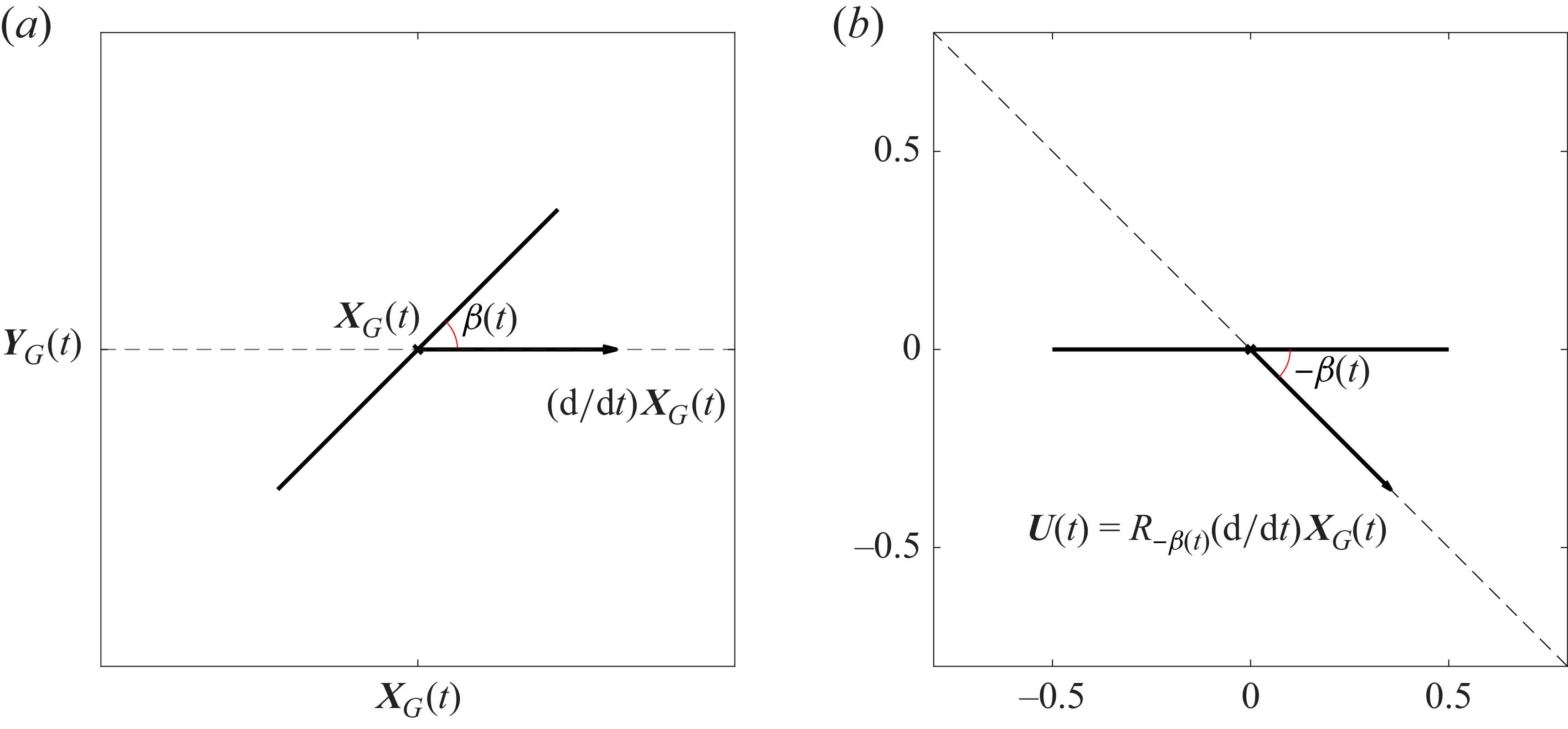
 (a)
 (b)
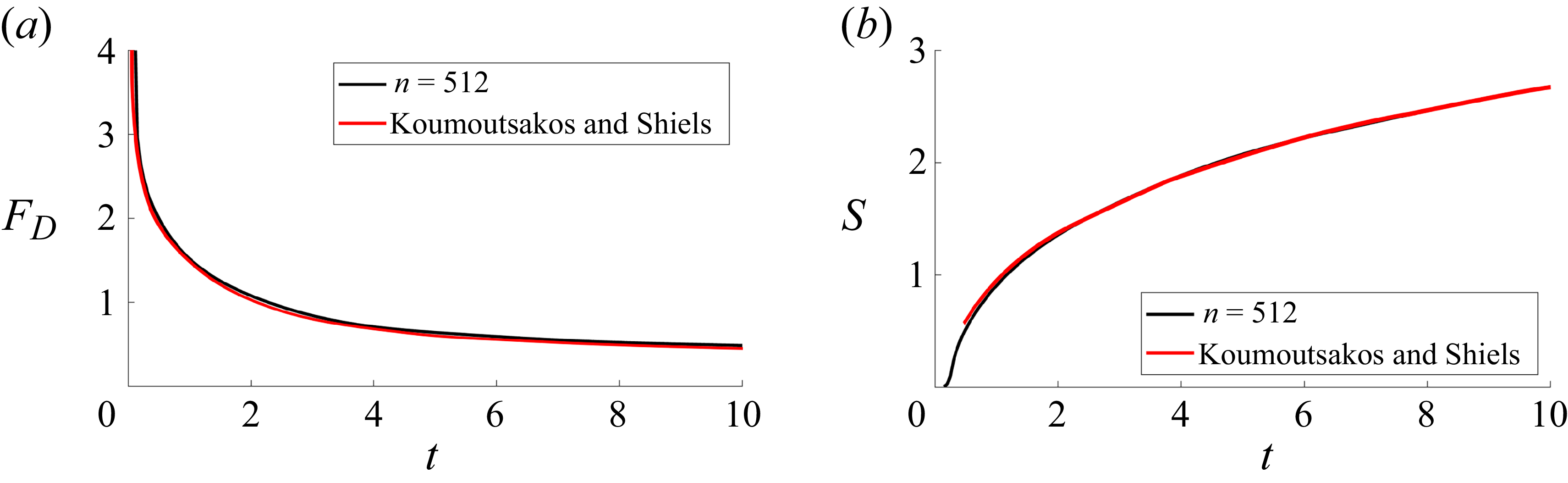
 FD
 S
 Re=1000
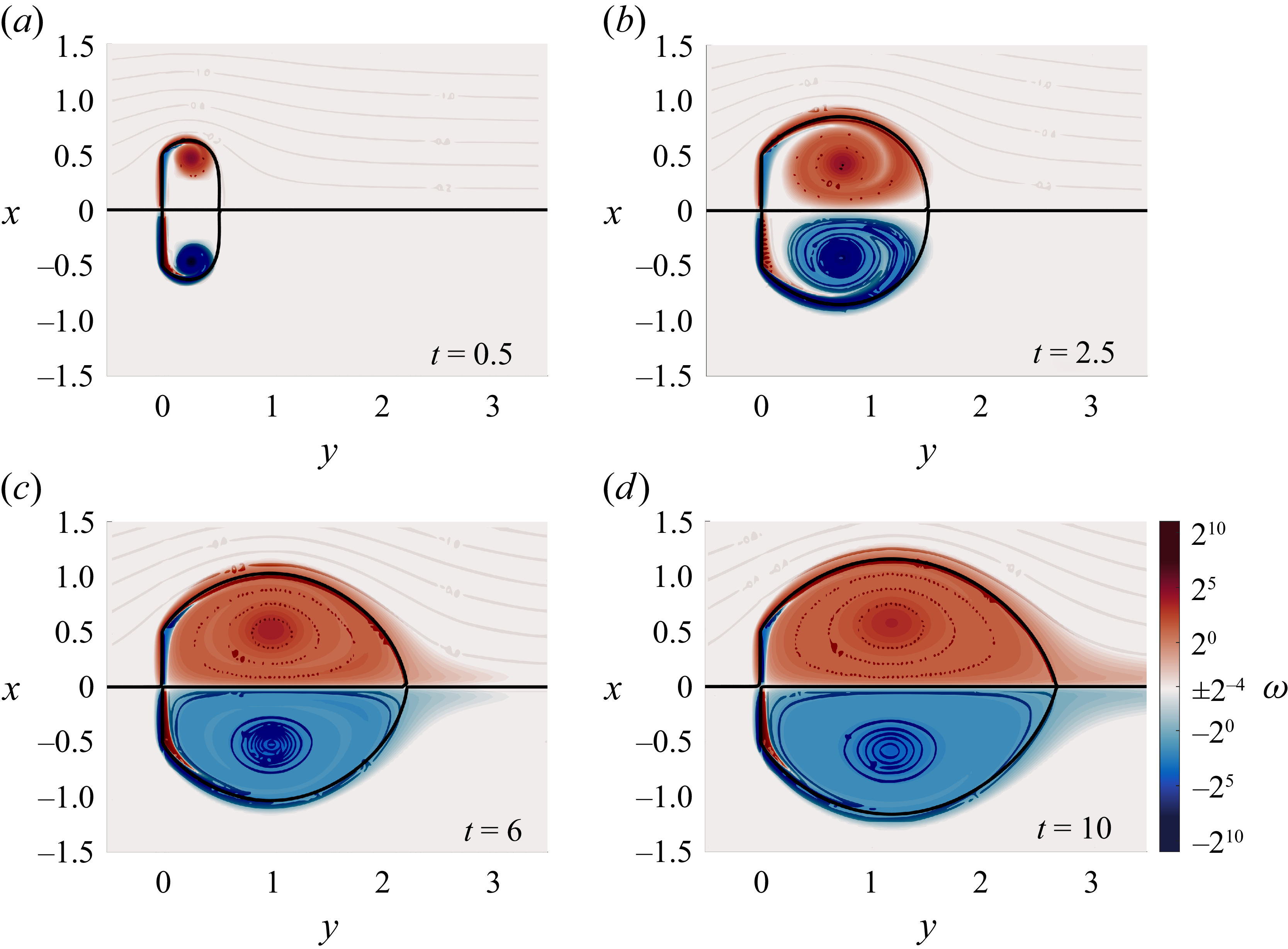
 t
 Re=1000
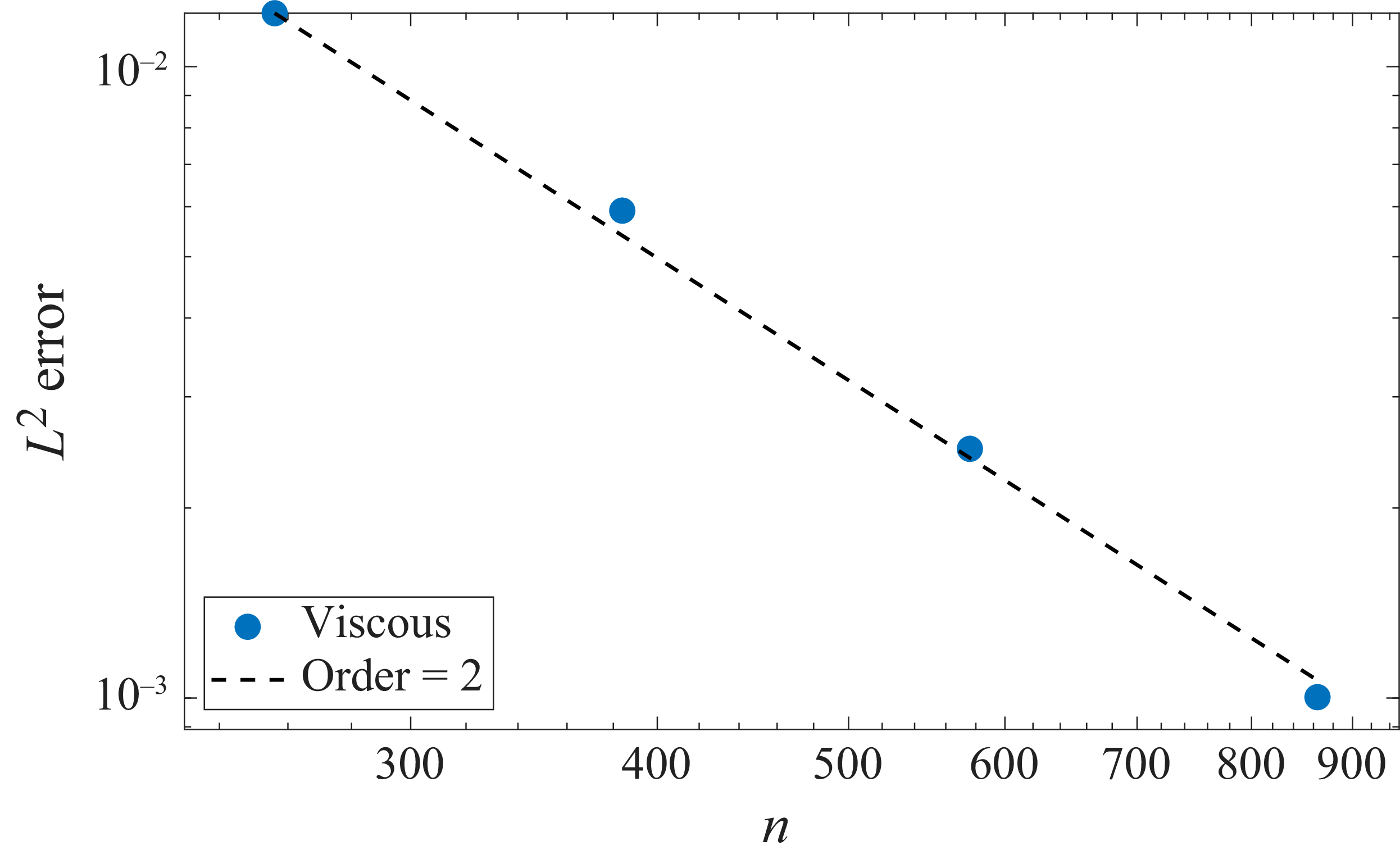
 L2
 n
 −2

 t
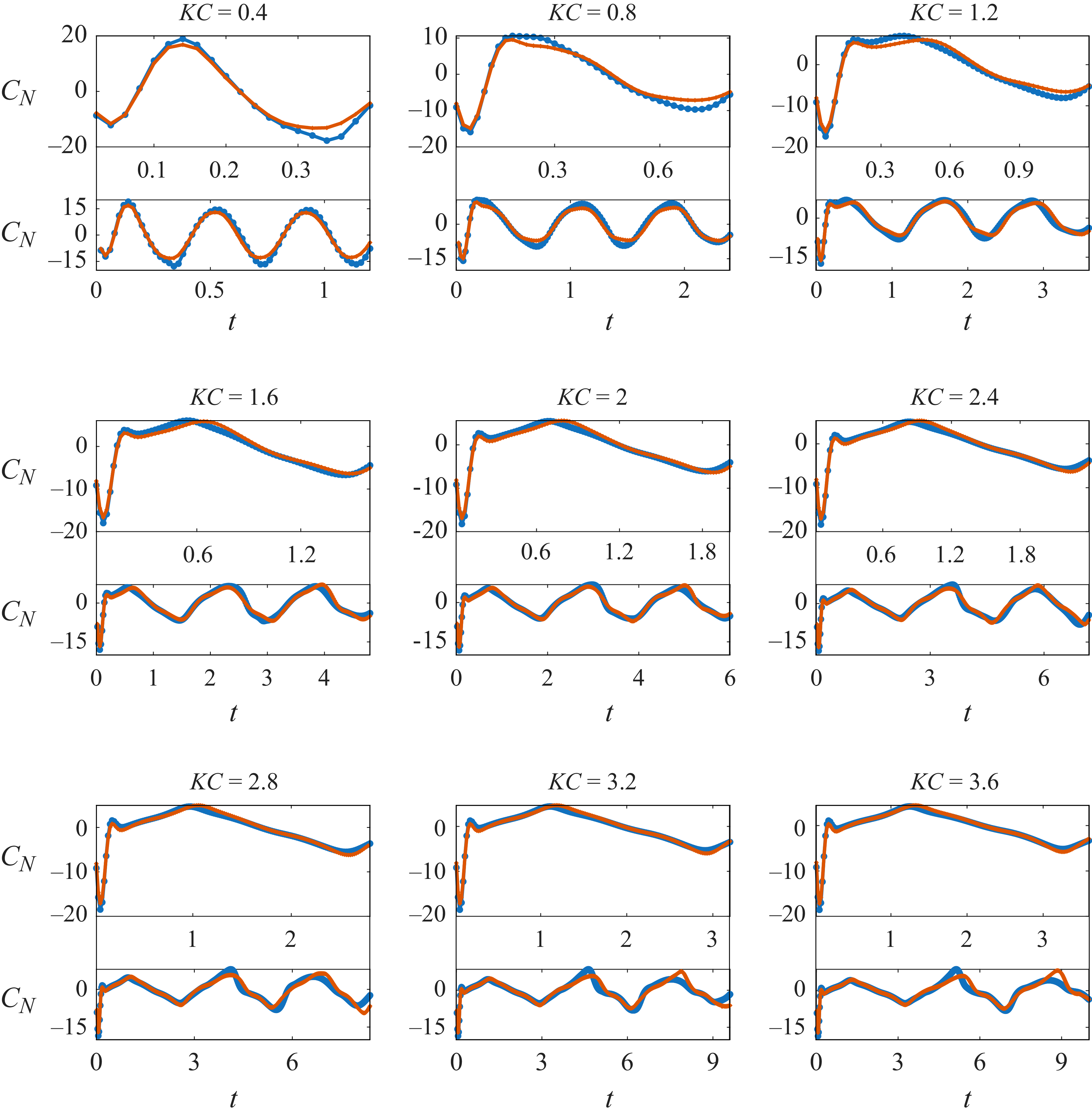
 t=KC
 t=3KC
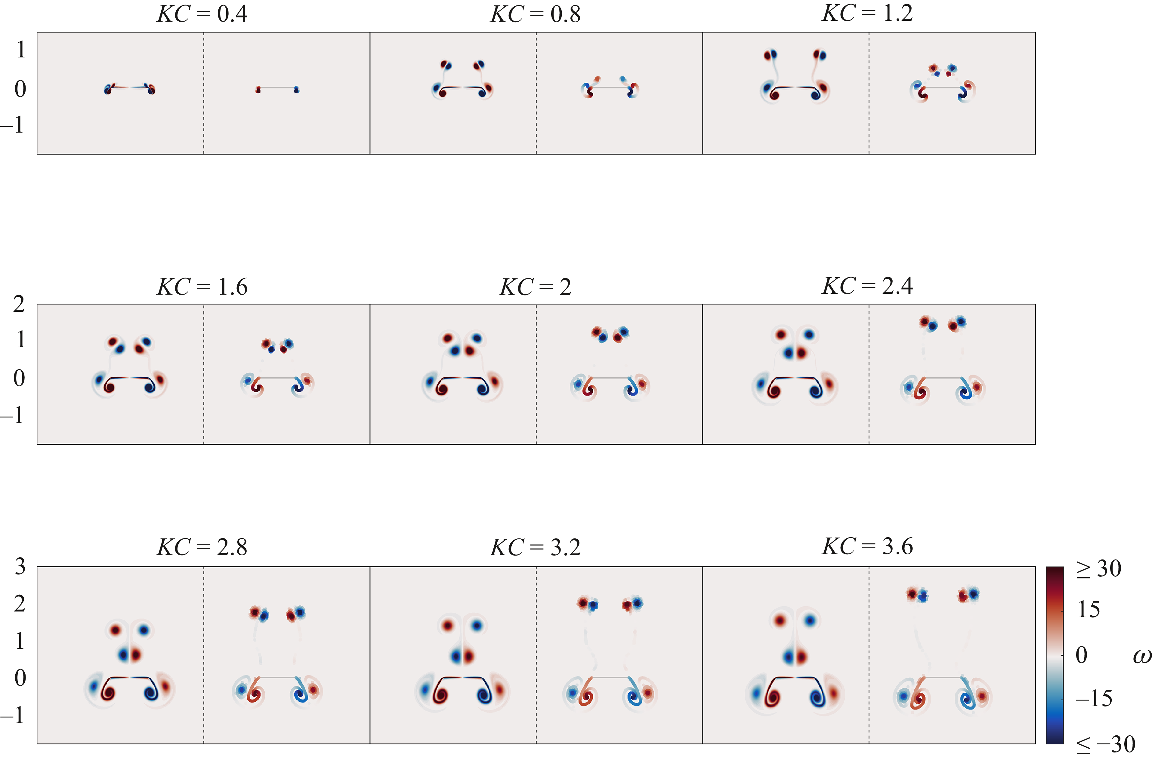
 ω
 t=KC
 KC=0.4,…,3.6
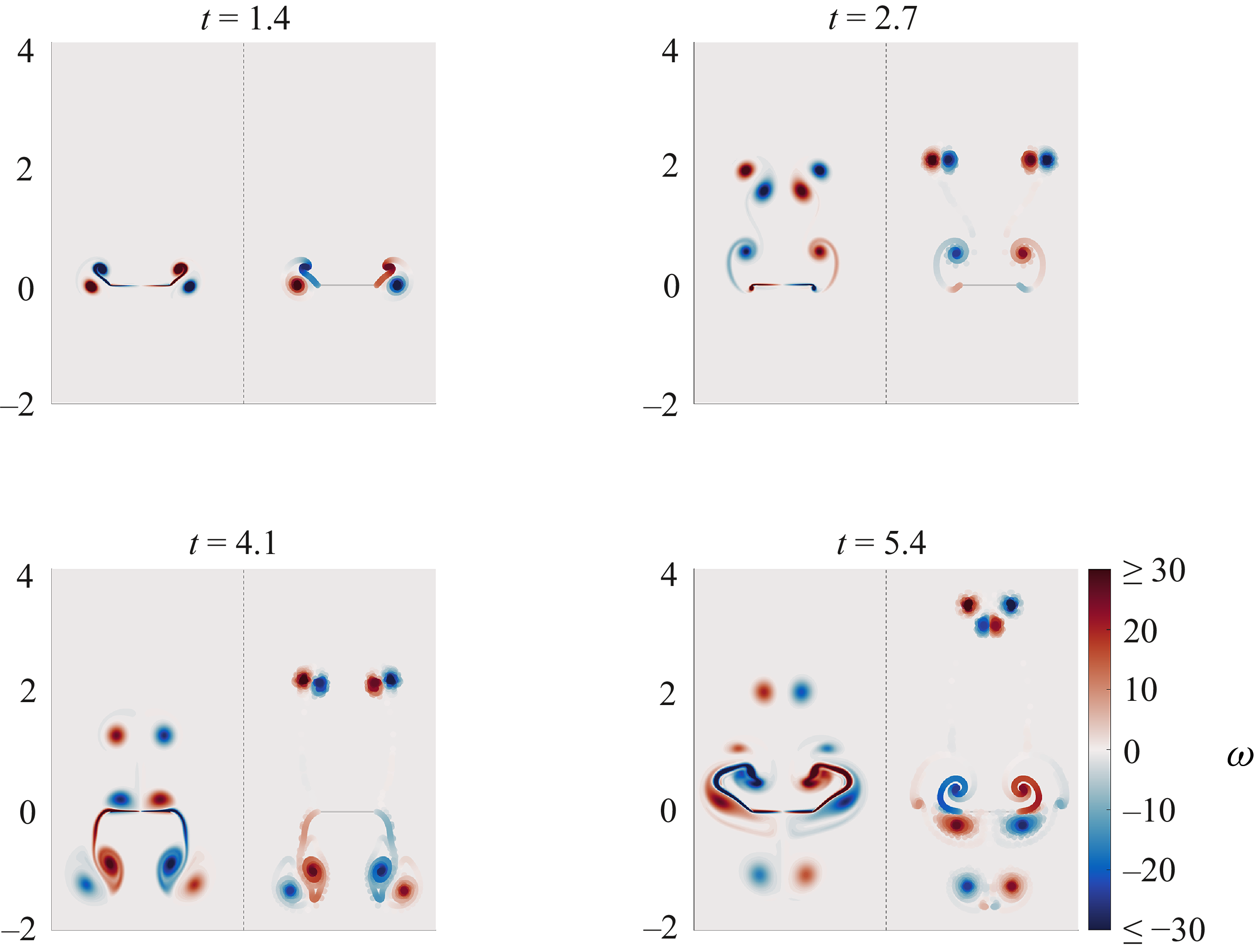
 t=1.4,2.7,4.1
 KC=3.6
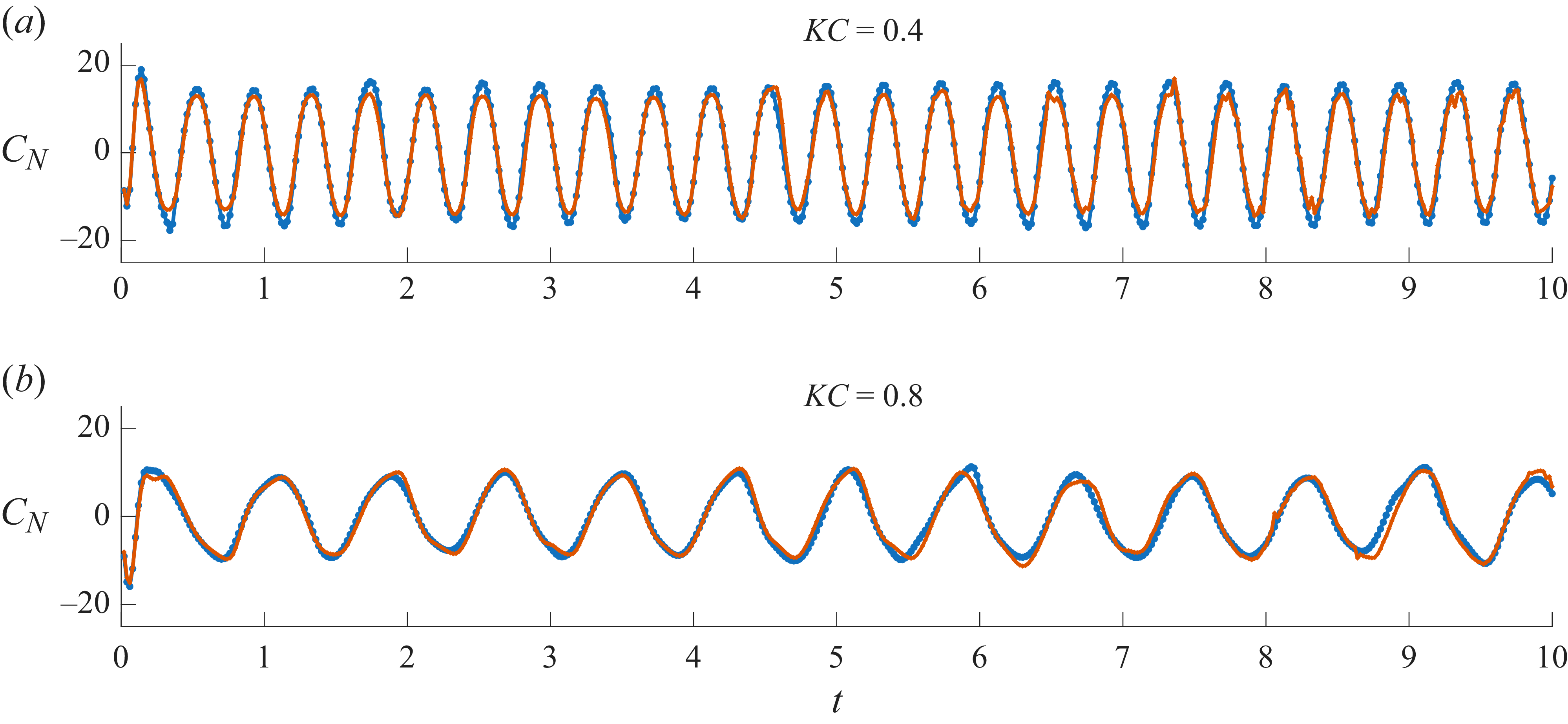
 CN
 t
 KC=0.4
 0.8
 t=10
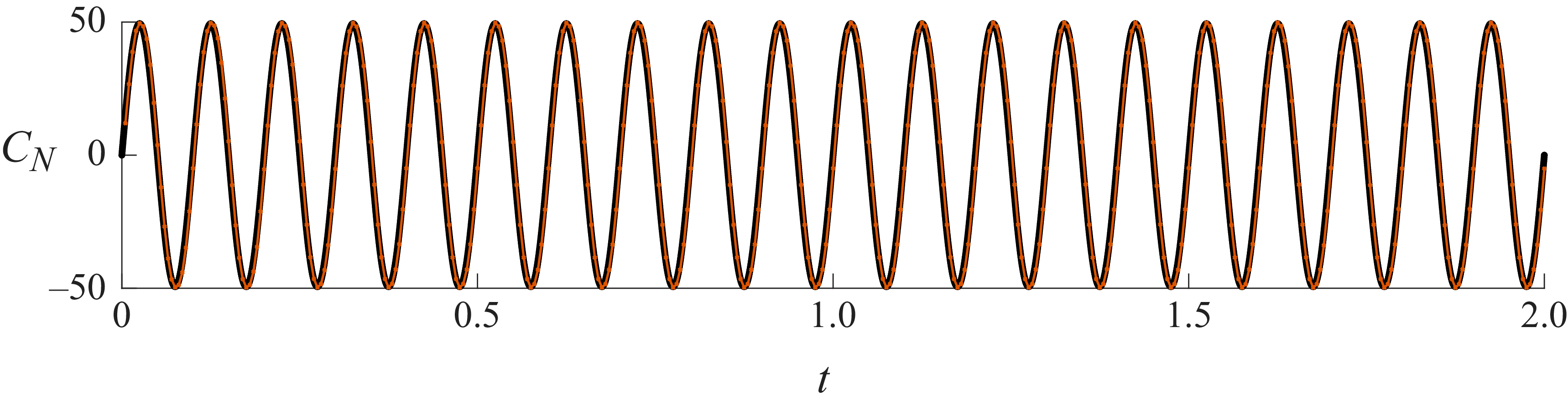
 CN
 t
 KC=0.1
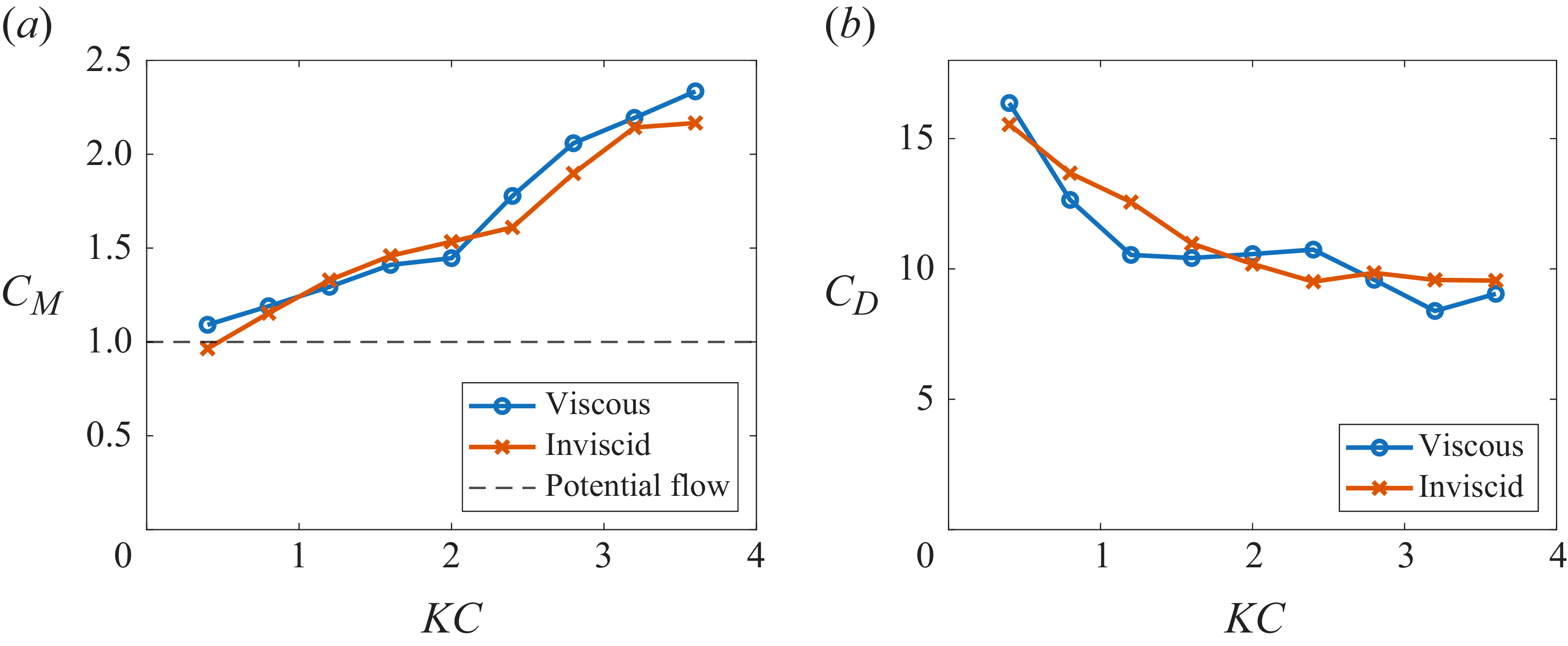
 CM
 CD
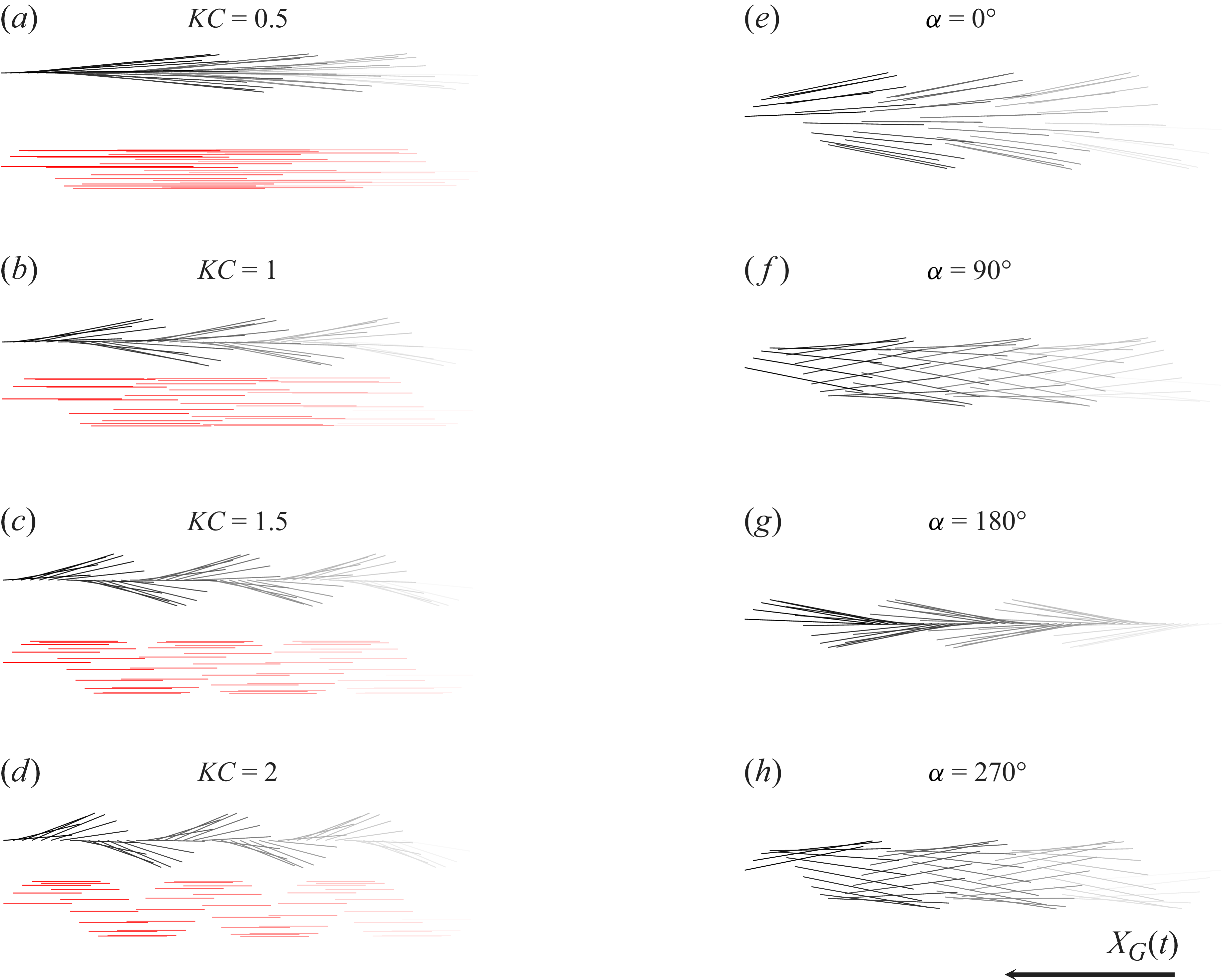
 KC=0.5,1,1.5,2
 St=0.4
 KC=1
 α=0∘,90∘,180∘,270∘

 St=0.2
 St=0.4
 CN
 t=KC
 t=3KC
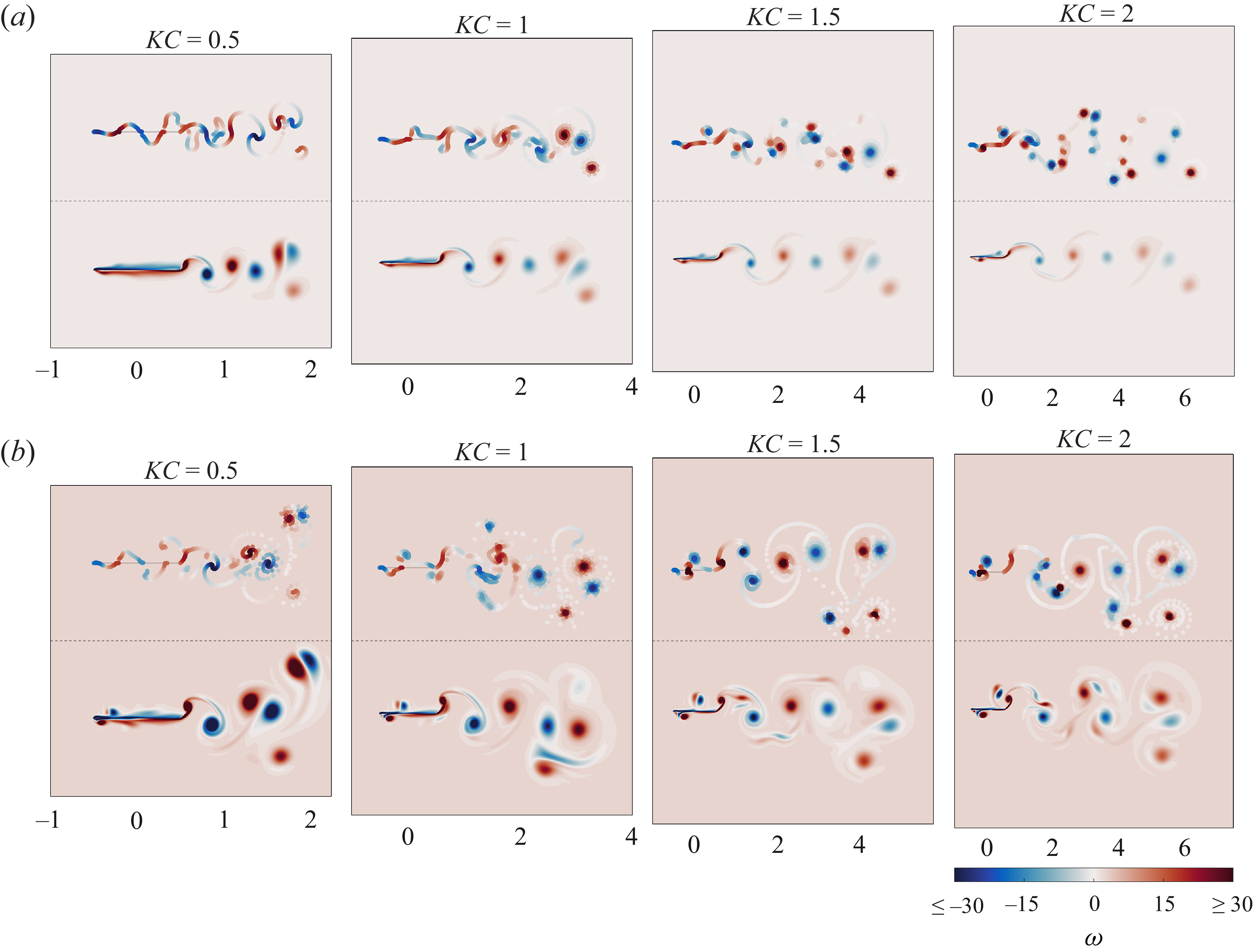
 ω
 t=3KC
 St=0.2
 St=0.4
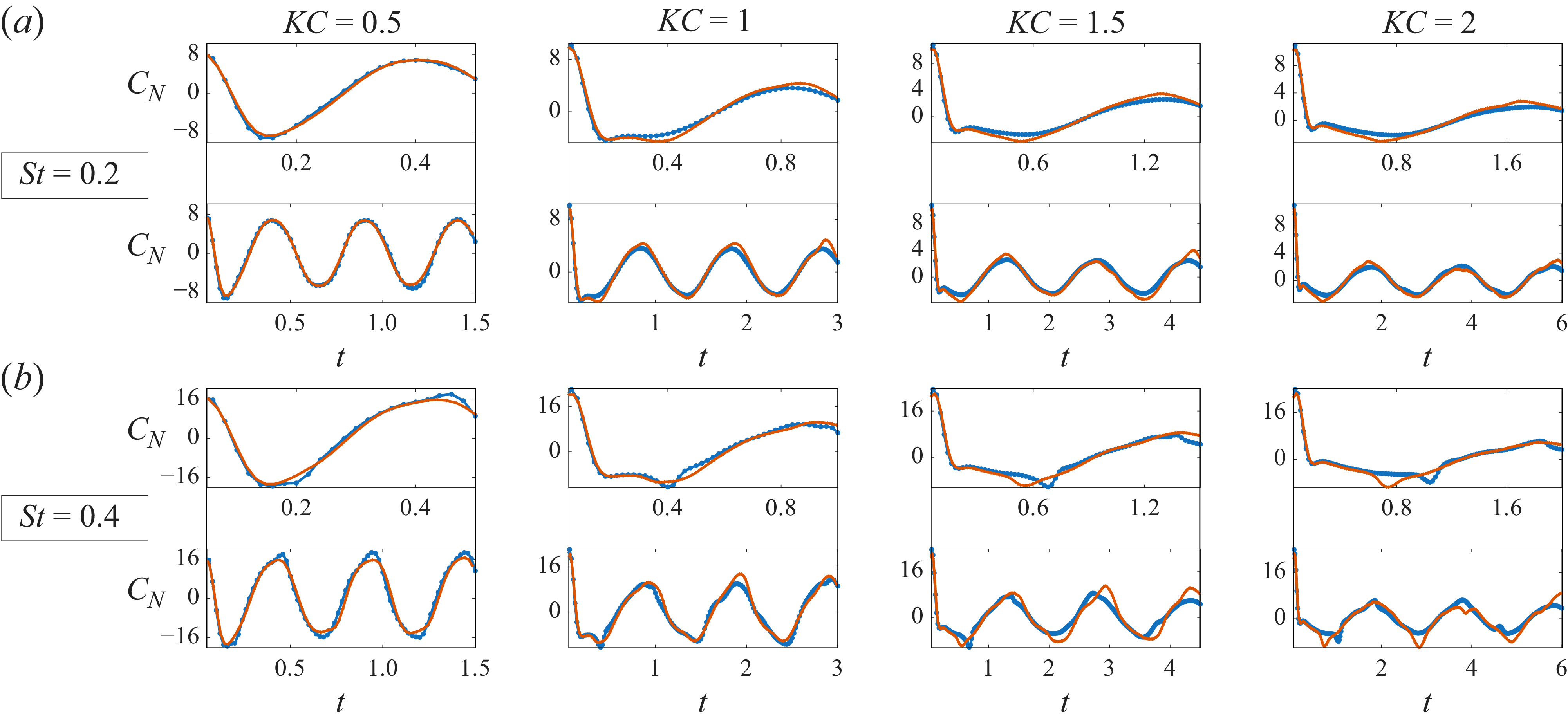
 St=0.2
 St=0.4
 CN
 t=KC
 t=3KC
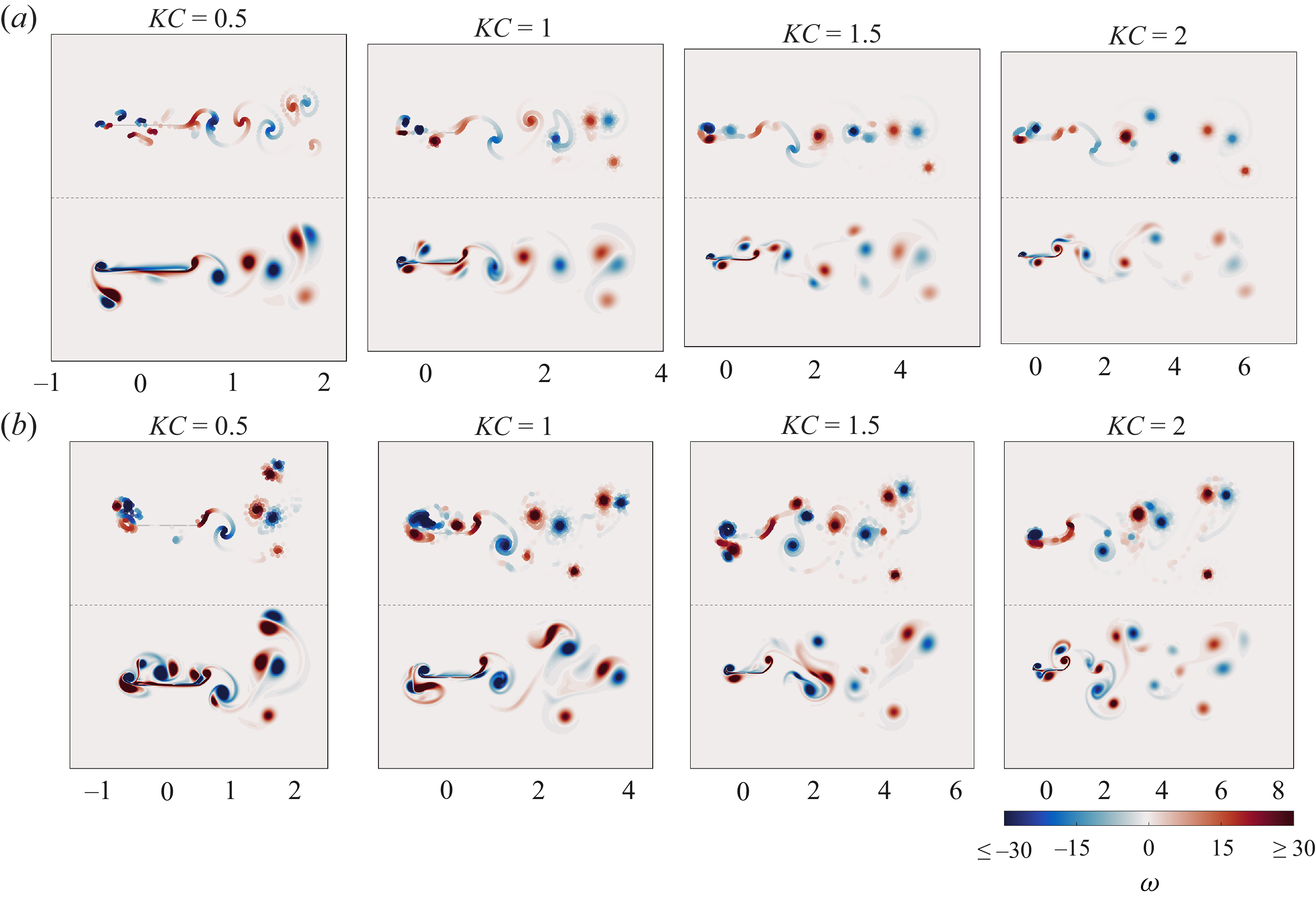
 ω
 t=3KC
 St=0.2
 St=0.4
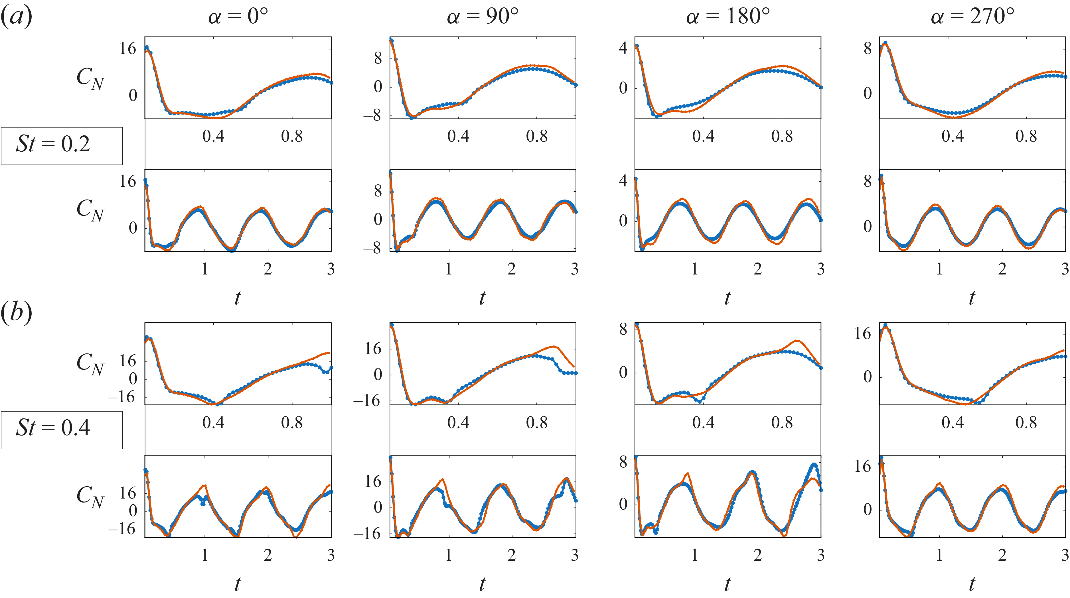
 KC=1
 α
 St=0.2
 St=0.4
 CN
 t=
 t=3
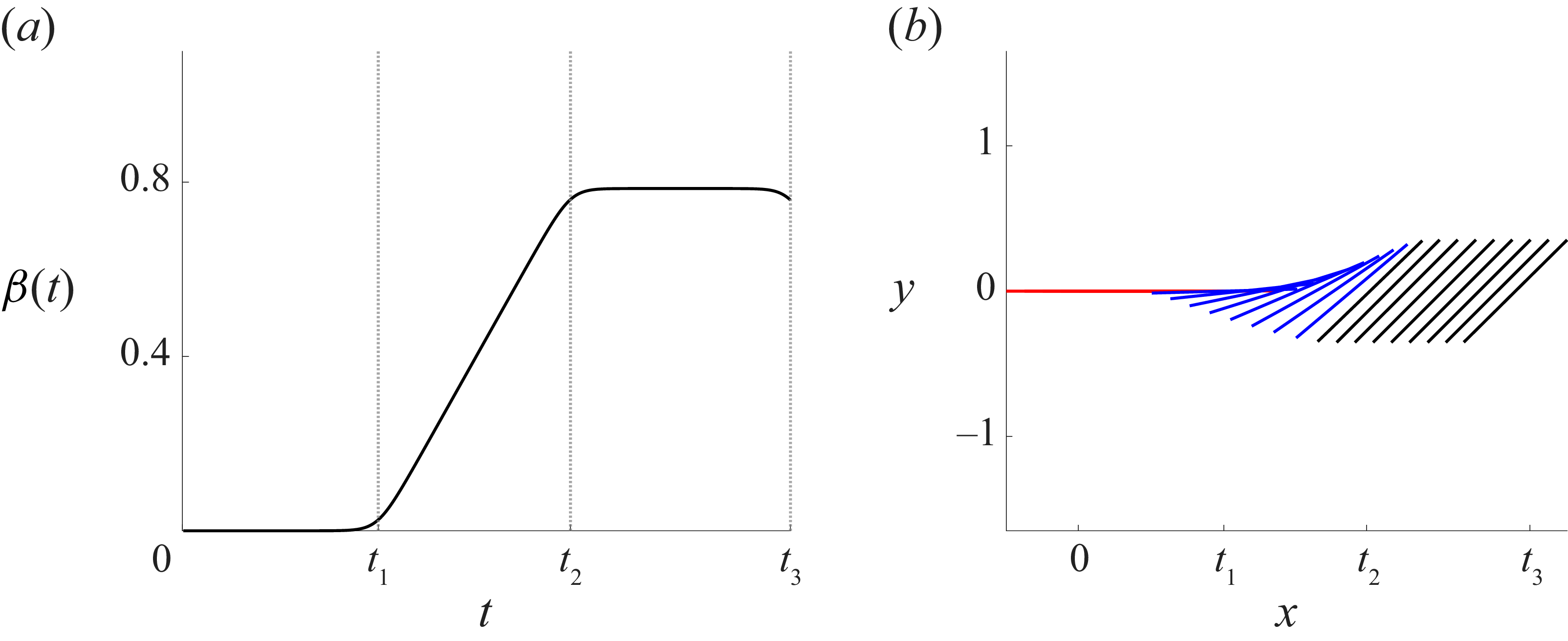
 β(t)
 Xp=0.5
 [0,t1],[t1,t2],[t2,t3]
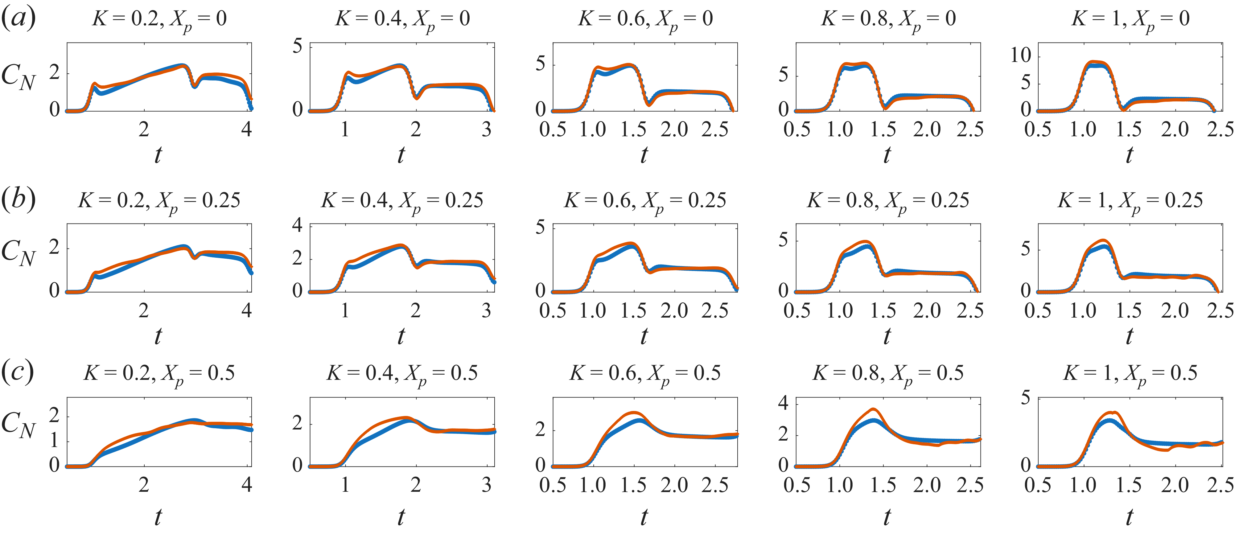
 t=t3
 K
 Xp
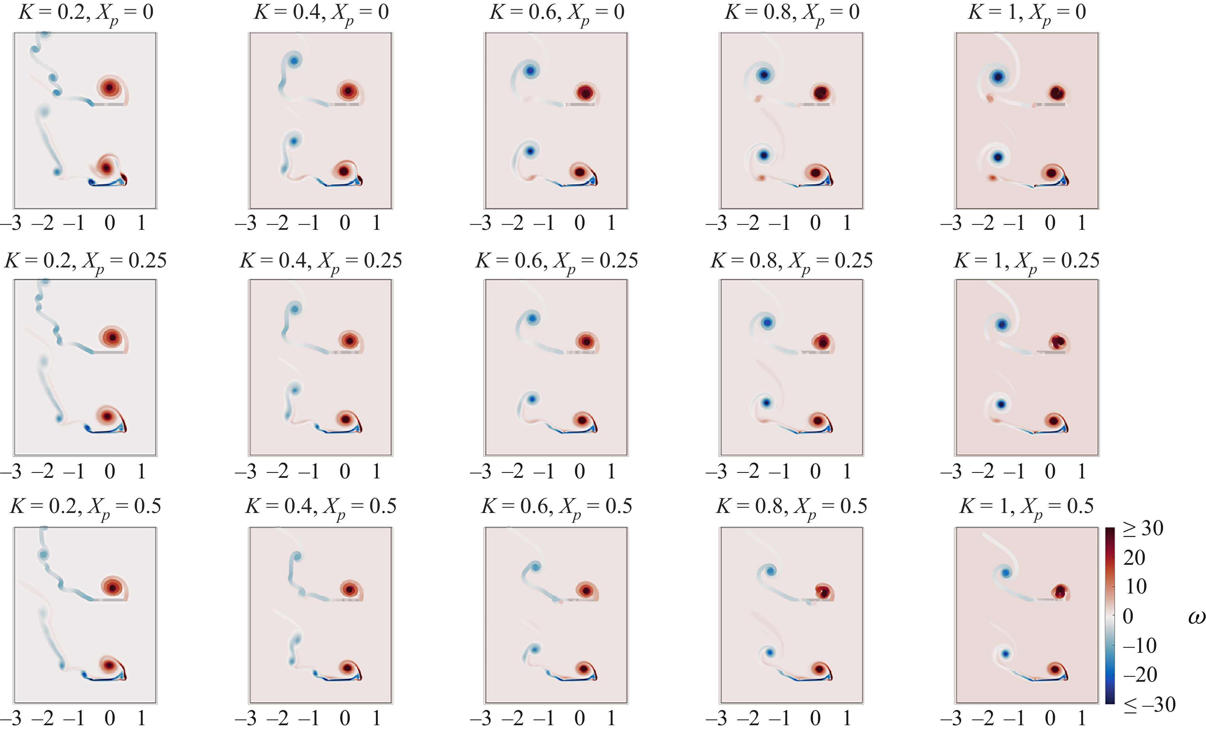
 ω
 t=t3
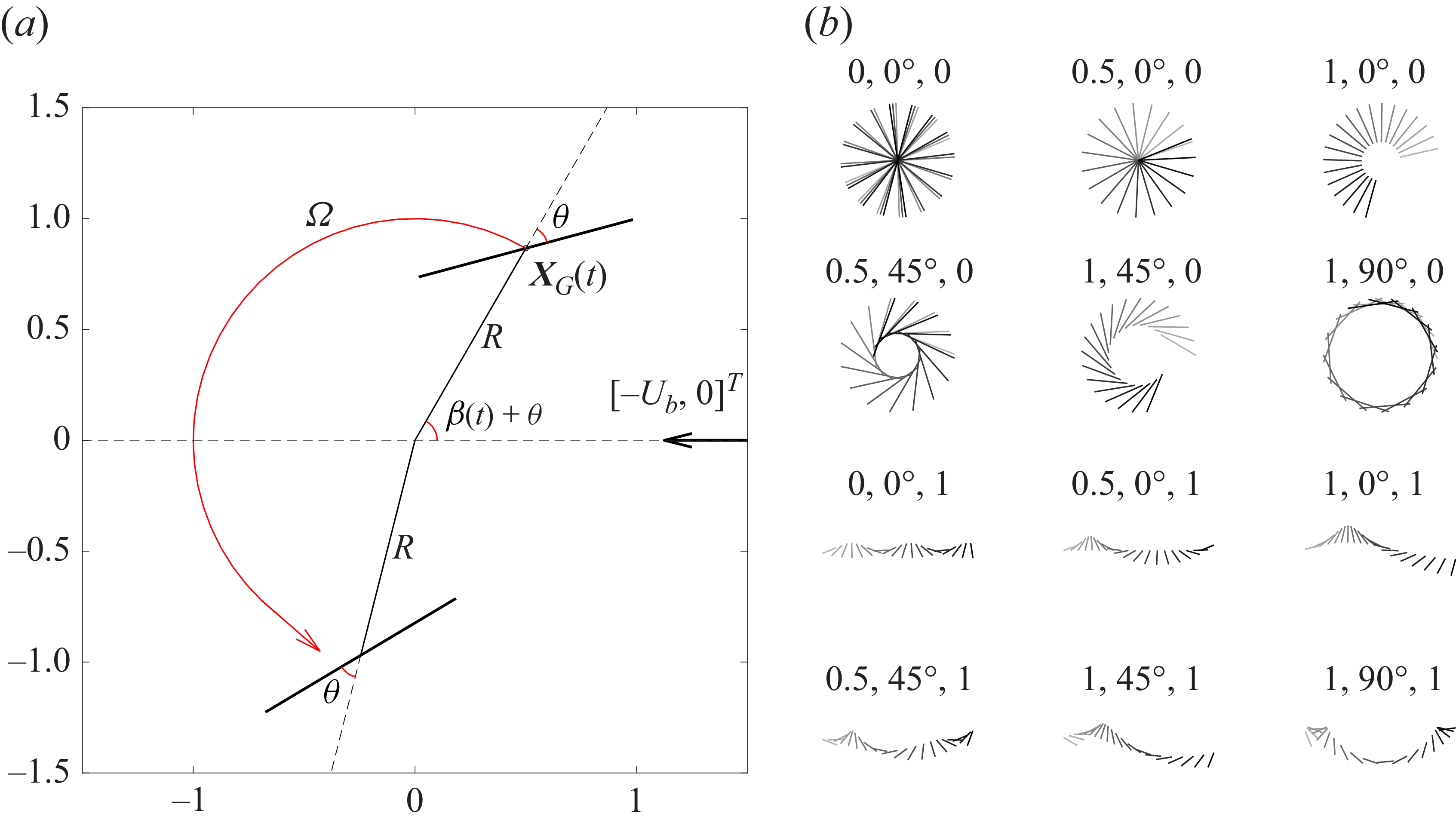
 Ω
 θ
 R
 [−Ub,0]T
 (R,θ,Ub)
 t=10

 t=10
 (R,θ)
 −Ub
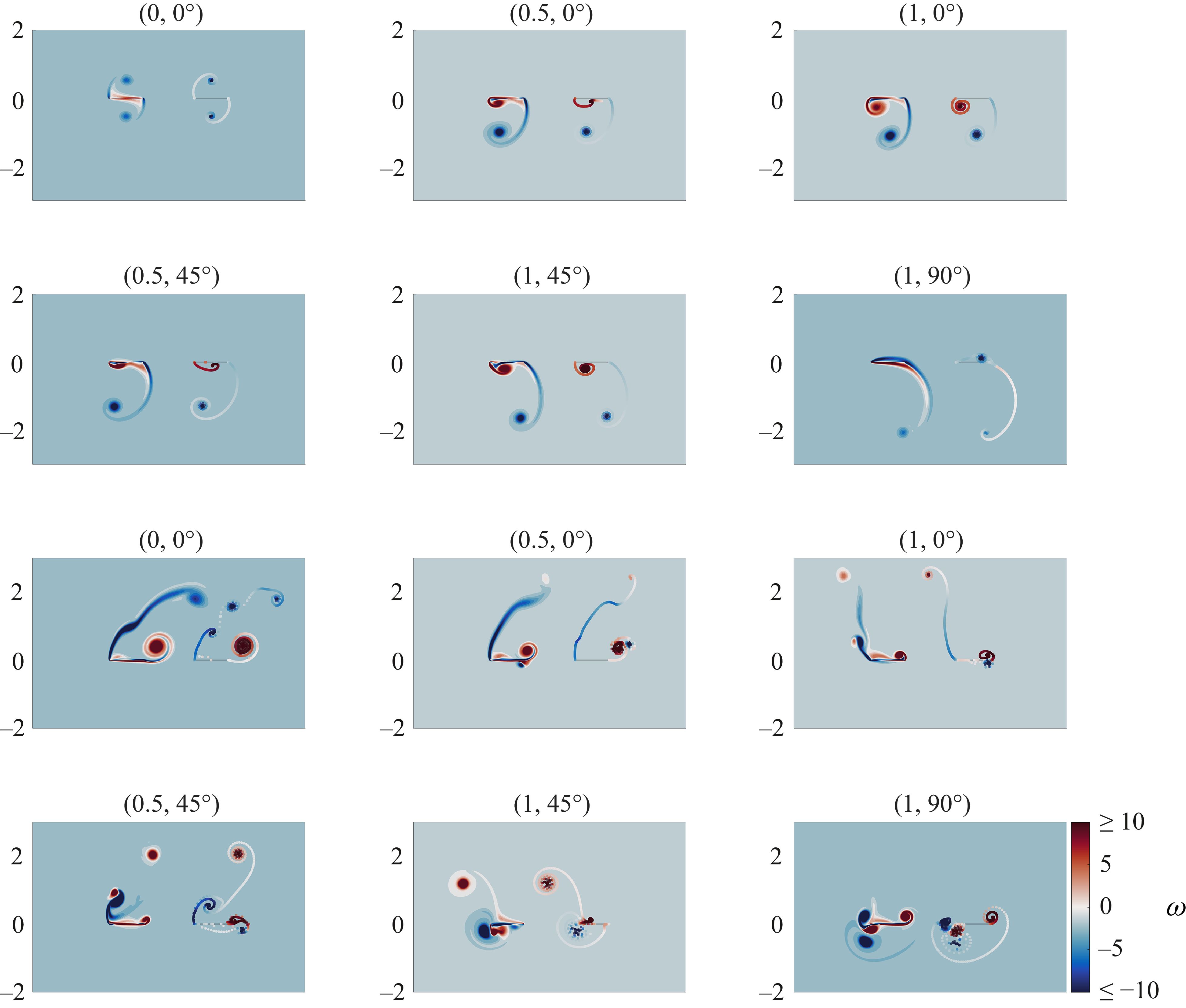
 ω
 t=4
 R
 θ
 Ub=0
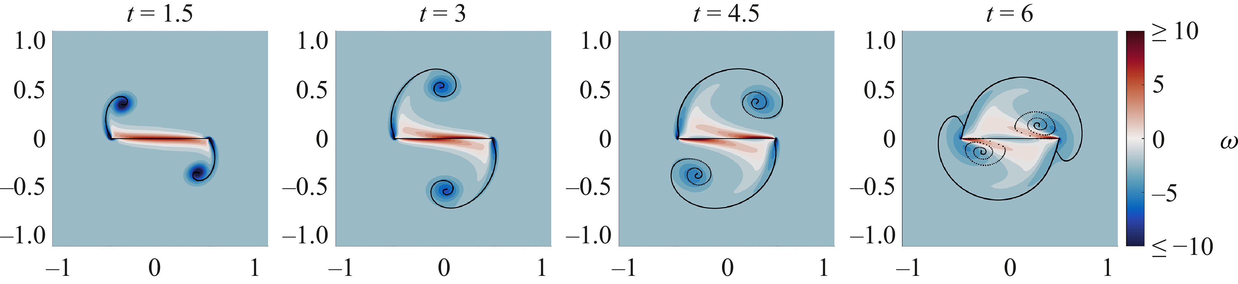
 ω
 t
 (R,θ,Ub)=(0,0∘,0)
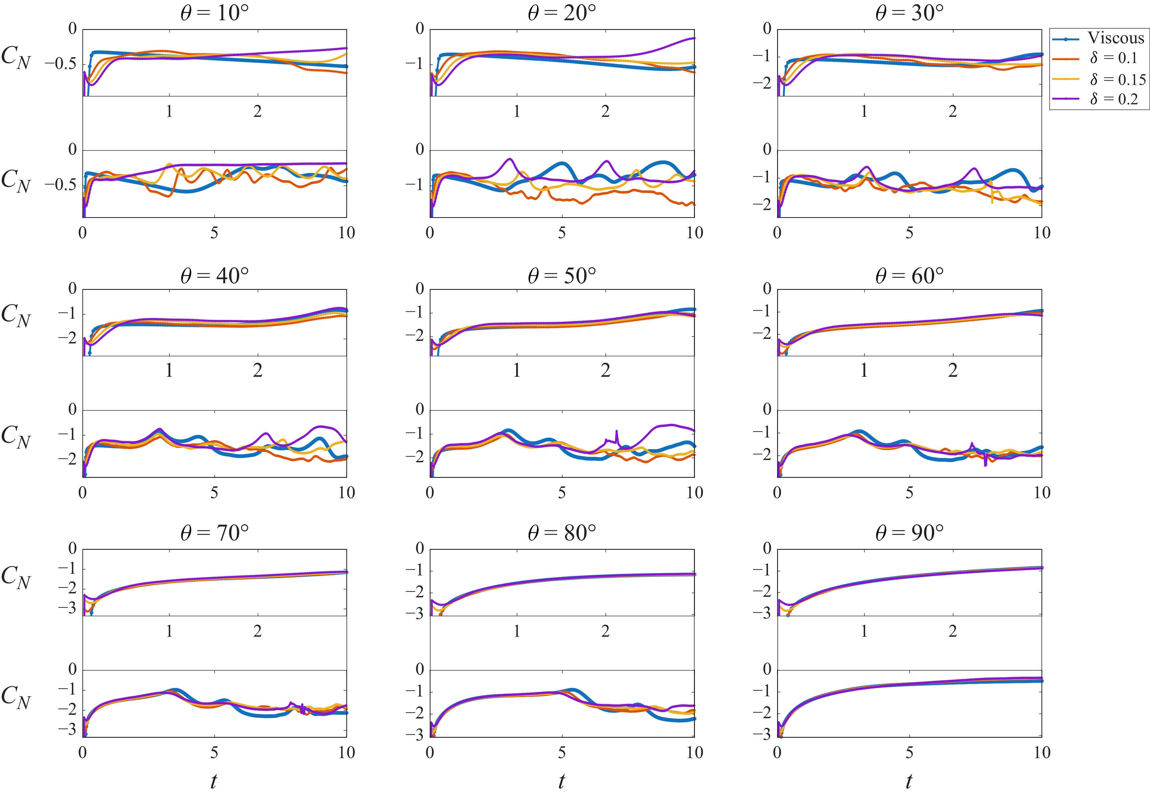
 θ=10∘,…,90∘
 x
 t=3
 t=10
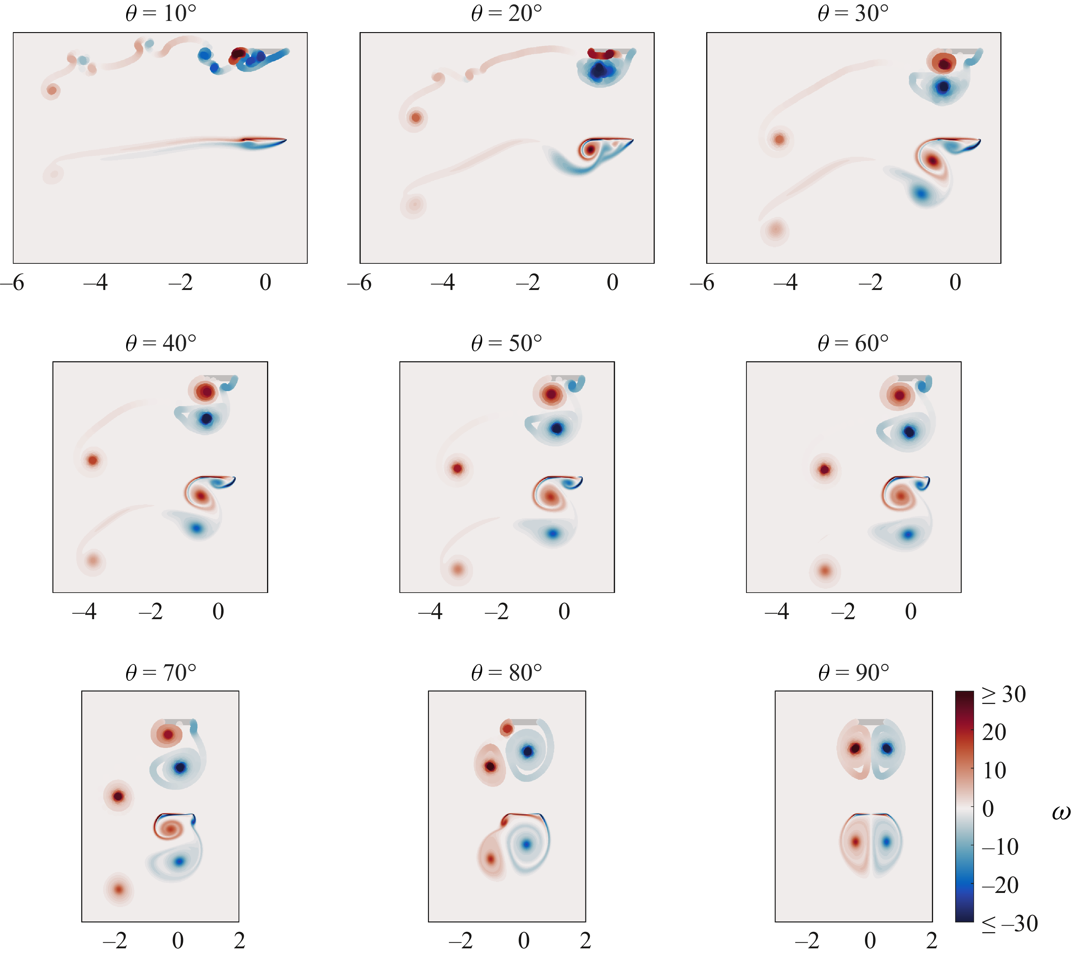
 ω
 t
 θ=10∘,…,90∘
 x
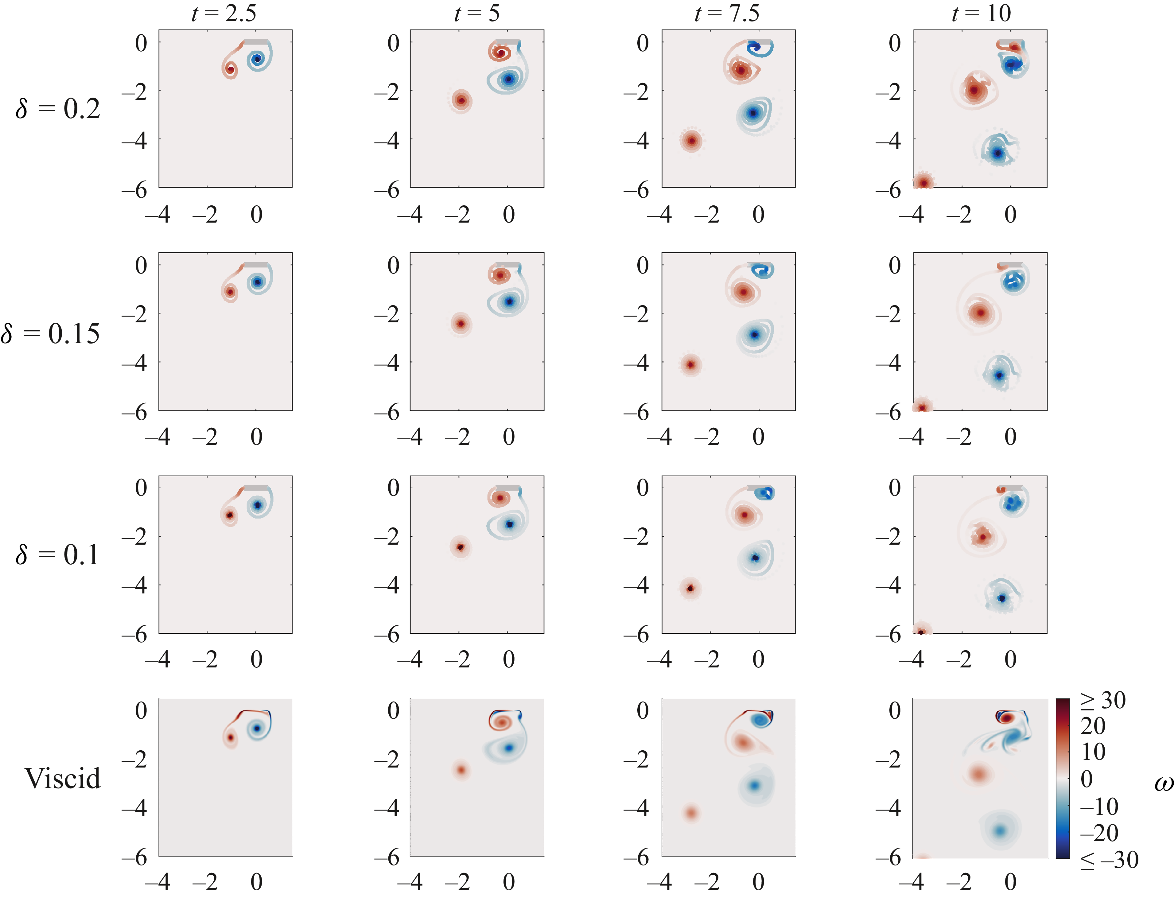
 ω
 t=2.5, 5, 7.5
 θ=70∘
 x
 δ=0.1,0.15,0.2
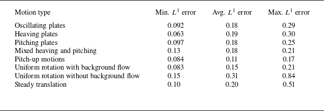
 L1
 L1
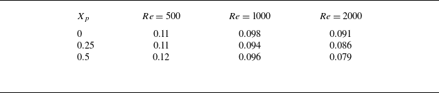
 L1
 Xp
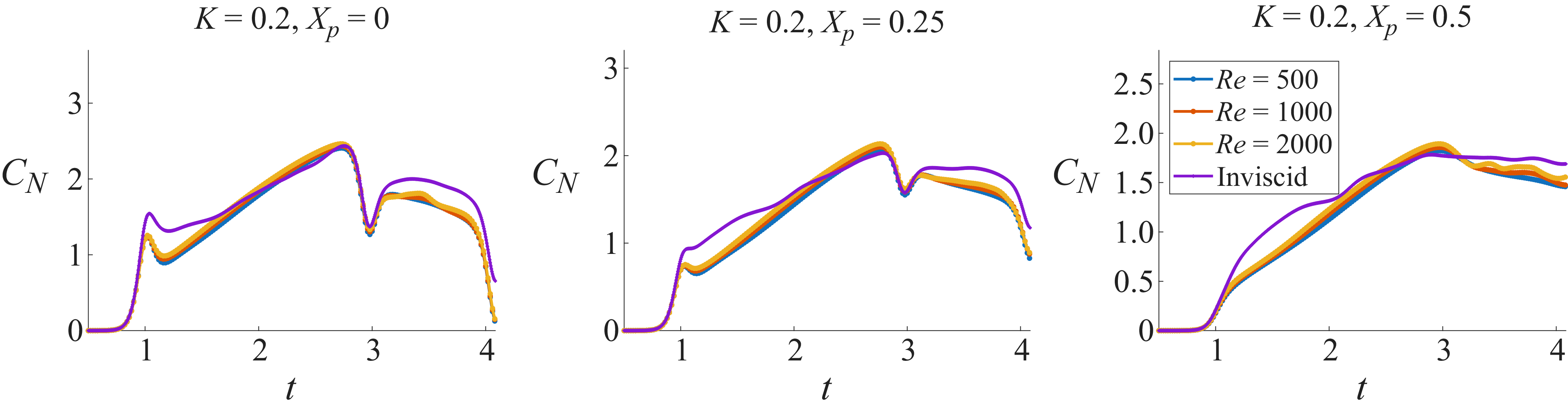
 Xp=0,0.25,0.5
 K=0.2
 Re=500,1000,2000
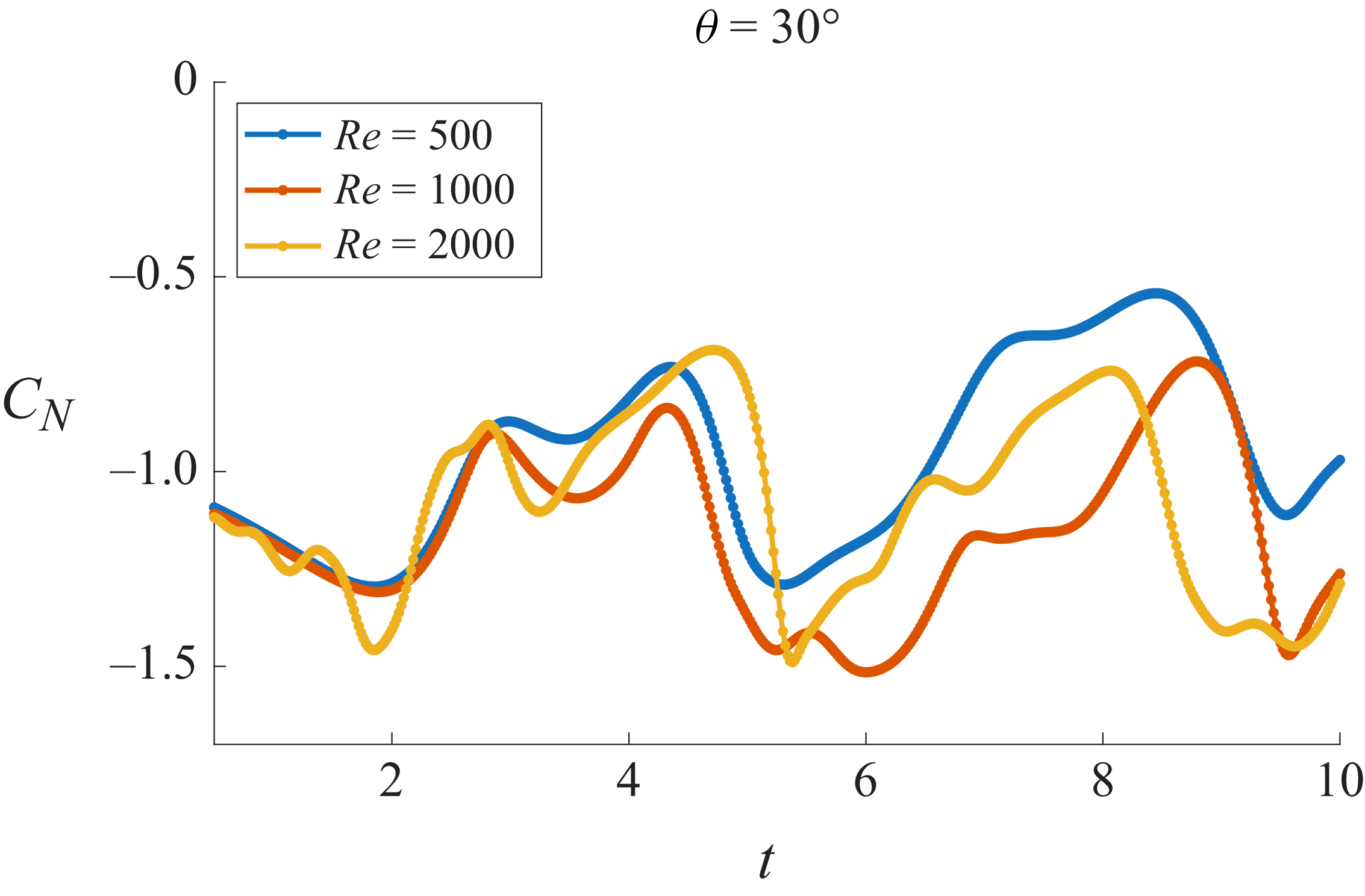
 CN
 θ=30∘
 Re=500,1000,2000
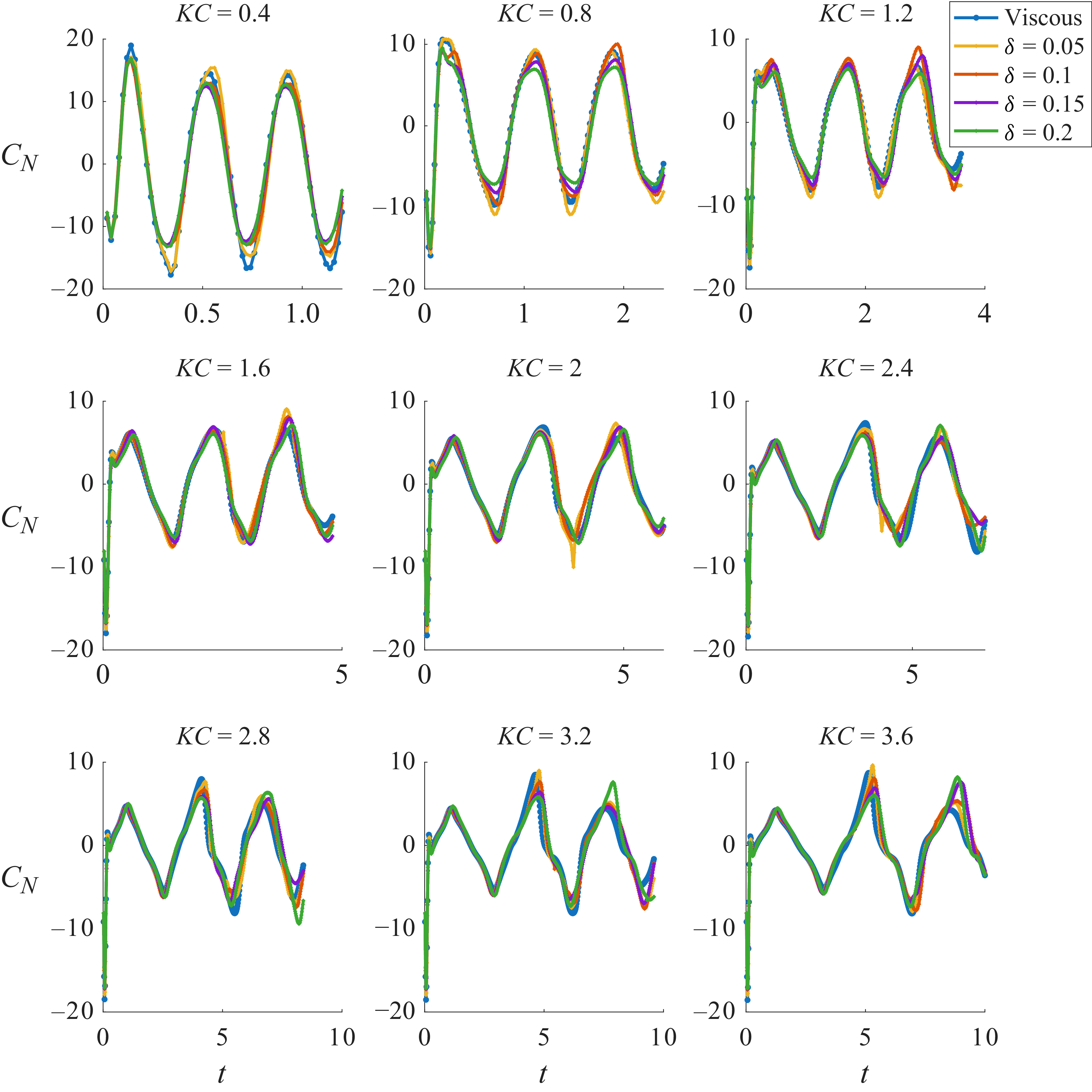
 CN
 δ=0.05,0.1,0.15,0.2
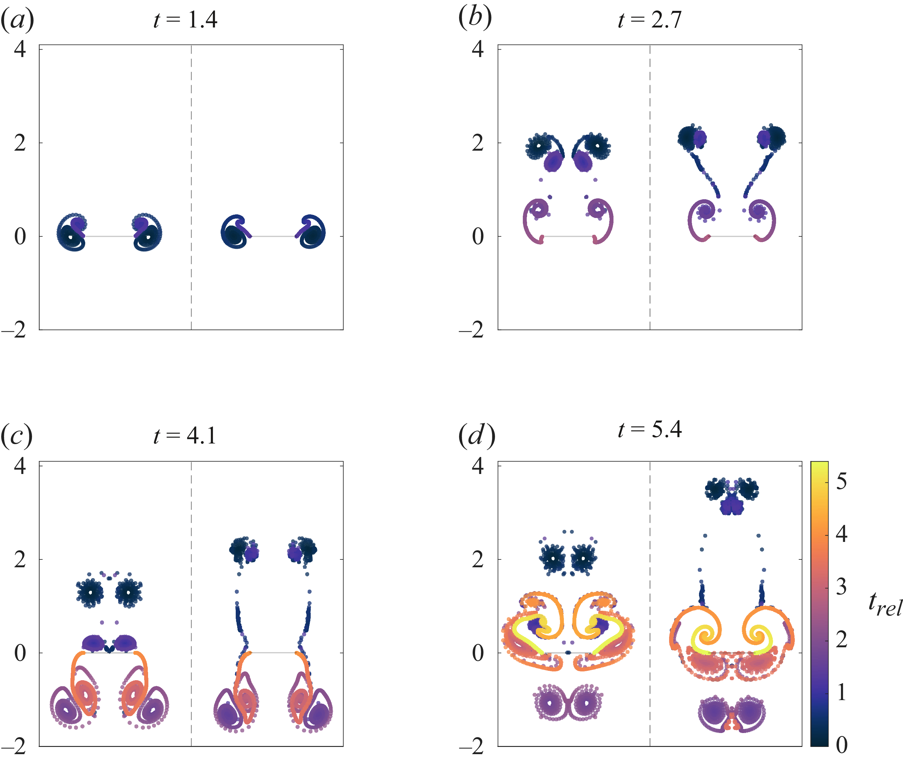
 t=1.4,2.7,4.1,5.4
 trel

 Open access

