2.1. Mathematical model for instability problem

2.1.1. Oscillatory Stokes flow

Stokes’ boundary layer theory has been effectively validated in characterising the influence of two lateral walls in the Hele-Shaw flow (Viola et al. Reference Viola, Gallaire and Dollet2017; Bongarzone et al. Reference Bongarzone, Jouron, Viola and Gallaire2023; Li & Li Reference Li and Li2024). The primary procedure is to derive the velocity profile along the gap direction and then calculate its spatial average to quantify the damping induced by the lateral confinement.

Under vertical periodic vibration, the effective gravitational acceleration is given by $G ( t' )=g-a\cos\, ( \varOmega t' )$ . Linearising the Navier–Stokes equations about the state of rest $\boldsymbol{U}'=0$ and $P' ( z',t' ) =-\rho G ( t' ) z'$ , the equations for the perturbation fields of velocity, $\boldsymbol{u}' ( x',y',z',t' ) = ( u',v',w' )^{\mathrm{T}}$ , and pressure, $p' ( x',y',z',t' )$ , within the fluid bulk read

(2.2) \begin{align} \frac {\partial \boldsymbol{u}'}{\partial t'}=-\frac {1}{\rho } \boldsymbol{\nabla }'\! p'+\nu {\boldsymbol{\nabla }'} ^2 \boldsymbol{u}',\quad \boldsymbol{\nabla }' \boldsymbol{\cdot } \boldsymbol{u}'=0. \end{align}

According to the feature of Faraday waves in Hele-Shaw cells, the gap is narrow enough that $bk\ll 1$ , with $k$ denoting the wavenumber. We assume that there are no flows along the $y'$ -direction and the velocity satisfies $v'=0$ . Equations (2.2) then reduce to

(2.3a) \begin{align} \frac {\partial u'}{\partial t'}=-\frac {1}{\rho } \frac {\partial p'}{\partial x'}+\nu \frac {\partial ^2 u'}{\partial y^{\prime 2}},& \quad \frac {\partial w'}{\partial t'}=-\frac {1}{\rho } \frac {\partial p'}{\partial x'}+\nu \frac {\partial ^2 w'}{\partial y^{\prime 2}}, \quad \frac {\partial p'}{\partial y'}=0, \\[-12pt]\nonumber \end{align}

(2.3b) \begin{align} &\frac {\partial u'}{\partial x'}+\frac {\partial w'}{\partial z'}=0. \end{align}

By making them dimensionless with the following expressions:

(2.4a–i) \begin{align} \begin{aligned} x=&\ kx',\quad y=\frac {y'}{b},\quad z=kz',\quad u=\frac {\varOmega u'}{g},\quad v=\frac {\varOmega v'}{bkg},\\ &w=\frac {\varOmega w'}{g},\quad p=\frac {k p'}{\rho g},\quad t=\varOmega t',\quad \zeta =k\zeta ', \end{aligned} \end{align}

the first two equations in (2.3a ) in dimensionless form become

(2.5a,b) \begin{align} \frac {\partial u}{\partial t}=- \frac {\partial p}{\partial x}+\frac {\delta _{St}^2}{2} \frac {\partial ^2u}{\partial y^2},\quad \frac {\partial w}{\partial t}=- \frac {\partial p}{\partial z}+\frac {\delta _{St}^2}{2} \frac {\partial ^2w}{\partial y^2}, \end{align}

where $\delta _{St}=\sqrt {2\nu /\varOmega } /b$ is the dimensionless thickness of the oscillating Stokes boundary layer (Bongarzone et al. Reference Bongarzone, Jouron, Viola and Gallaire2023).

Because the Faraday waves observed in Hele-Shaw cell experiments possess a subharmonic oscillation at a frequency of $\varOmega /2$ (Li et al. Reference Li, Li, Li, Liao and Chen2019b ), only the fundamental mode is considered, which is reflected in the separated exponential part of solutions associated with periodicity. Therefore, the ansatzes can be written as $\boldsymbol{u} ( x,y,z,t )=\text{Re} [ \tilde {\boldsymbol{u}} ( x,y,z ) e^{\mathrm{i}t/2 } ]$ and $p ( x,z,t )=\text{Re} [ \tilde {p} ( x,z ) e^{\mathrm{i}t/2 } ]$ . Substituting them into (2.5a , b ), together with the no-slip condition at $y=\pm 1/2$ , the resulting ordinary differential equations about $y$ are solved. Then we have

(2.6a,b) \begin{align} \tilde {u} =2\mathrm{i} \left \{ 1-\frac {\cosh \left [ \left ( 1+\mathrm{i} \right )y/\delta _1 \right ] }{\cosh \left [ \left ( 1+\mathrm{i} \right ) /2\delta _1 \right ] } \right \} \frac {\partial \tilde {p} }{\partial x},\quad \tilde {w} =2\mathrm{i} \left \{ 1-\frac {\cosh \left [ \left ( 1+\mathrm{i} \right )y/\delta _1 \right ] }{\cosh \left [ \left ( 1+\mathrm{i} \right ) /2\delta _1 \right ] } \right \} \frac {\partial \tilde {p} }{\partial z}, \end{align}

where $\delta _1=\delta _{St}/\sqrt {1/2}$ is a modified dimensionless Stokes boundary layer thickness specific to the fundamental wave mode.

By integrating (2.6a , b ) along the $y'$ -direction and taking the average, the gap-averaged velocity components $\bar {u}$ and $\bar {w}$ are expressed by the two-dimensional pressure field $\bar {p}$ , namely

(2.7a,b) \begin{align} \bar {u}\left ( x,z,t \right ) =\lambda _1 \frac {\partial \bar {p}}{\partial x},\quad \bar {w}\left ( x,z,t \right ) =\lambda _1 \frac {\partial \bar {p}}{\partial z}, \end{align}

with

(2.8) \begin{align} \lambda _1=2\mathrm{i} \left \{ 1-\left ( 1-\mathrm{i} \right )\delta _1 \tanh \left [ \left ( 1+\mathrm{i} \right )/2\delta _1 \right ] \right \}\!. \end{align}

After this gap-averaging process, the Hele-Shaw flow reduces to the two-dimensional dynamics in the $x'$ $z'$ plane and the dissipation resulting from the lateral walls is implicitly incorporated in the coefficient $\lambda _1$ .

2.1.2. Governing equations

The dimensionless continuity equation of (2.3b ), when gap-averaged and combined with (2.7a , b ), is simplified to a Laplace equation for the pressure field

(2.9) \begin{align} \frac {\partial ^2 \bar {p}}{\partial x^2}+\frac {\partial ^2 \bar {p}}{\partial z^2} =0. \end{align}

The dimensionless non-penetrable boundary condition at the solid bottom reads

(2.10) \begin{align} \frac {\partial \bar {p}}{\partial z}=0,\quad \text{at } \quad z=-\infty . \end{align}

Assuming that the location of the bottom extends to $z=-\infty$ is feasible since the experimental liquid layer is sufficiently deep and $kH\gg 1$ with $H$ denoting the liquid depth.

On the moving free surface, the normal stress is balanced by the capillary force. We mention here the Taylor expansion of boundary conditions on the free surface around $z'=0$ and, following elimination of the nonlinear terms, the normal stress boundary condition reads

(2.11) \begin{align} -p'+\rho G\left ( t' \right ) \zeta '+2 \mu \frac {\partial w'}{\partial z'}=\sigma \left ( \frac {\partial ^2 \zeta '}{\partial x^{\prime 2}} +\frac {\partial ^2 \zeta '}{\partial y^{\prime 2}}\right )\!,\quad \text{at } \quad z'=0, \end{align}

where $\sigma$ is the surface tension coefficient. The right-hand side of (2.11) represents the capillary force, incorporating curvature contributions from two principal directions. Because only the Faraday wave profile is considered in the current section (that is, only $\bar {\zeta }'$ in (2.1) is preserved), the meniscus curvature term $\partial ^2 \zeta '/\partial y^{\prime 2}$ in (2.11) should be removed. After turning into dimensionless form using (2.4a – i ) and gap averaging in the $y'$ -direction, the boundary condition (2.11) becomes

(2.12) \begin{align} -\bar {p}+\left ( 1- \frac {a}{g}\cos t \right ) \bar {\zeta }+\delta _{St}^2k^2b^2\lambda _1\frac {\partial ^2 \bar {p}}{\partial z^2}=l_c^2 k^2\frac {\partial ^2 \bar {\zeta }}{\partial x^2}, \quad \text{at } \quad z=0, \end{align}

where $l_c=\sqrt {\sigma /\rho g}$ denotes the capillary length, and $\bar {\zeta }$ represents the gap-averaged two-dimensional Faraday wave profile that has been made dimensionless with $\bar {\zeta }=k\bar {\zeta }'$ . In (2.12), the viscous stress reflected by the term $\partial ^2 \bar {p}/\partial z^2$ is retained. Although the previous theory indicates that the effect of fluid viscosity on dissipation in the Hele-Shaw system can be neglected (Li & Li Reference Li and Li2024), and this viscous term, scaling as $\delta _{St}^2k^2b^2\ll 1$ , has been ignored by Li et al. (Reference Li, Li and Liao2019a ) and Bongarzone et al. (Reference Bongarzone, Jouron, Viola and Gallaire2023), we retain it to preserve the fidelity of damping representation, with a detailed discussion on this viscous dissipation later.

The second boundary condition on the free surface is the linearised kinematic condition, whose dimensionless form is

(2.13) \begin{align} \frac {\varOmega ^2}{gk}\frac {\partial \zeta }{\partial t}=w,\quad \text{at } \quad z=0. \end{align}

After gap averaging, (2.13) reduces to

(2.14) \begin{align} \frac {\varOmega ^2}{gk}\frac {\partial \bar {\zeta }}{\partial t}=\lambda _1\frac {\partial \bar {p}}{\partial z},\quad \text{at } \quad z=0. \end{align}

The system of equations (2.9), (2.10), (2.12) and (2.14) constitutes the governing equations for the Faraday instability problem in Hele-Shaw cells under the oscillatory Stokes flow approximation.

2.2. Asymptotic expansion

The derivation of amplitude equations is a classical method to describe pattern selection beyond linear instability (see, for instance, the frameworks of Milner (Reference Milner1991), Chen & Viñals (Reference Chen and Viñals1999) and Westra et al. (Reference Westra, Binks and Van De Water2003)). This approach is also applied to obtain the critical condition for linear Faraday instability in Hele-Shaw cells (Rajchenbach et al. Reference Rajchenbach, Leroux and Clamond2011; Li et al. Reference Li, Li and Liao2019a ). Inspired by these studies, we derive the amplitude equation from the reestablished mathematical model given in § 2.1.2.

By introducing an expansion parameter $\epsilon$ , the physical parameters can be expressed by

(2.15a–c) \begin{align} a=\epsilon \hat {a},\quad \delta _{St}^2k^2b^2=\epsilon \hat {\delta },\quad \lambda _1=2\mathrm{i}\big( 1-\epsilon \hat {\delta }_1 \big), \end{align}

where $\epsilon \hat {\delta }_1= ( 1-\mathrm{i} )\delta _1 \tanh [ ( 1+\mathrm{i} )/2\delta _1 ]$ is the damping part of $\lambda _1$ . To examine the variation of variables in a long time scale, in the spirit of multiple scale analysis (Nayfeh Reference Nayfeh1993), a slow time scale $T=\epsilon t$ is introduced, and naturally $\partial _t \to \partial _t+\epsilon \partial _T$ . Then the rescaled governing equations read

(2.16a) \begin{align} &\def\lumina\hspace{11.5pc} \frac {\partial ^2 \bar {p}}{\partial x^2} +\frac {\partial ^2 \bar {p}}{\partial z^2}=0, \\[-12pt]\nonumber \end{align}

(2.16b) \begin{align} &-\bar {p}+\left ( 1- \epsilon \frac {\hat {a}}{g} \cos t \right ) \bar {\zeta }+ \epsilon \hat {\delta } 2\mathrm{i}\big ( 1-\epsilon \hat {\delta }_1 \big )\frac {\partial ^2 \bar {p}}{\partial z^2} =l_c^2 k^2\frac {\partial ^2 \bar {\zeta }}{\partial x^2},\quad \text{at } \quad z=0, \\[-12pt]\nonumber \end{align}

(2.16c) \begin{align} &\def\lumina\hspace{3.5pc} 4\omega ^2\big ( 1+l_c^2k^2 \big) \left ( \frac {\partial \bar {\zeta }}{\partial t} +\epsilon \frac {\partial \bar {\zeta }}{\partial T} \right )=2\mathrm{i}\big ( 1-\epsilon \hat {\delta }_1 \big) \frac {\partial \bar {p}}{\partial z},\quad \text{at } \quad z=0, \\[-12pt]\nonumber \end{align}

(2.16d) \begin{align} &\def\lumina\hspace{10pc} \frac {\partial \bar {p}}{\partial z}=0,\quad \text{at } \quad z=-\infty . \end{align}

In (2.16c ), the angular frequency has been non-dimensionalised with the expression $\varOmega /2=\omega \sqrt {gk+\sigma k^3/\rho }$ . We shall define $\omega _0$ as the limit of response frequency $\omega$ when $\epsilon =0$ with expansion $\omega ^2 = \omega _0^2 + \epsilon \omega _1^2$ . The variables in (2.16a )–(2.16d ) are expanded as follows:

(2.17a,b) \begin{align} \bar {p}=\bar {p}_1 + \epsilon \bar {p}_2 + \textit {O} ( \epsilon ^2 ),\quad \bar {\zeta }=\bar {\zeta }_1 + \epsilon \bar {\zeta }_2 + \textit {O} ( \epsilon ^2 ). \end{align}

According to these definitions, we find that $\bar {p}\sim \textit {O} (1)$ , $\bar {\zeta }\sim \textit {O} (1)$ , $a \sim \textit {O} (\epsilon )$ , $\delta _{St}^2k^2b^2 \sim \textit {O} (\epsilon )$ and the damping part of $\lambda _1$ is of the order $\sim \textit {O} (\epsilon )$ . In the absence of external forcing, the solutions corresponding to the static state are trivial, namely $\bar {\zeta }_s=0$ and $\bar {p}_s=0$ . Thus, the expansions in (2.17a , b ) refer exclusively to the perturbed components.

The equations at each order are solved analytically; details are provided in Appendix A.1. At order $\epsilon$ , a solvability condition arises from the Fredholm alternative, yielding

(2.18) \begin{align} \frac {\mathrm{d} A}{\mathrm{d} T} +\frac {1}{2} \left[ \mathrm{i} \big ( \hat {\delta }_{1,r}+\mathrm{i} \hat {\delta }_{1,i} \big)+\mathrm{i}\omega _1^2+2\hat {\delta } \right] A+\frac {\mathrm{i}\hat {a}}{4g\left ( 1+l_c^2k^2 \right ) }A^*=0, \end{align}

where $\hat {\delta }_{1,r}$ and $\hat {\delta }_{1,i}$ are the real and imaginary parts of $\hat {\delta }_1$ , respectively, $A(T)$ represents the complex amplitude of the linear Faraday wave on the slow time scale $T$ and the asterisk superscript ( $*$ ) designates the complex conjugate.

Equation (2.18) is the amplitude equation for the Faraday instability problem that incorporates dissipation from both the confinement of the lateral walls and the viscous stress, but excludes capillary damping induced by the contact angle dynamics. To derive an explicit expression of the damping, we decompose the complex amplitude $A$ into a modulus and phase, namely $A=|A |e^{\mathrm{i}\varPhi _A (T )}$ , and write the modulus as $|A |=A_0 e^{-\gamma _1 t}$ . The damping rate $\gamma _1$ and phase $\varPhi _A (T )$ are then given by

(2.19a) \begin{align} \gamma _1 &= -\frac {\mathrm{d} \log \left ( \left | A \right | /A_0 \right ) }{\mathrm{d} t} =-\frac {\epsilon }{\left | A \right | }\frac {\mathrm{d}\left | A \right | }{\mathrm{d}T} =\frac {1}{2} \big (\! - \delta _{1,i} +2\delta _{St}^2k^2b^2 \big ), \\[-12pt]\nonumber \end{align}

(2.19b) \begin{align} &\qquad \qquad \qquad \frac {\mathrm{d} \varPhi _A \left (T \right )}{\mathrm{d} T} =-\frac {1}{2} \big ( \hat {\delta }_{1,r} + \omega _1^2 \big ), \end{align}

where $\delta _{1,r}$ and $\delta _{1,i}$ denote the real and imaginary parts of $ ( 1-\mathrm{i} )\delta _1 \tanh [ ( 1+\mathrm{i} )/2\delta _1 ]$ , respectively, and are associated with the gap-averaged damping. The last term $\delta _{St}^2k^2b^2$ in (2.19a ) reflects the viscous dissipation arising from the normal stress boundary condition (2.11). Equation (2.19b ) indicates the frequency shift introduced by the Stokes flow approximation.

3.1. Incorporating meniscus effects into gap-averaged equations

If we take the meniscus $\eta '$ into account and substitute (2.1) into (2.11), another gap-averaged normal stress boundary condition is obtained as

(3.1) \begin{align} -\bar {p}+\left ( 1- \frac {a}{g}\cos t \right ) \bar {\zeta }+\delta _{St}^2k^2b^2\lambda _1\frac {\partial ^2 \bar {p}}{\partial z^2}=l_c^2 \left ( k^2\frac {\partial ^2 \bar {\zeta }}{\partial x^2}+\frac {2}{b^2}\left . \frac {\partial \eta }{\partial y} \right |_{y=1/2} \right )\!,\ \ \text{at } \ \ z=0, \end{align}

where $\eta '$ has been non-dimensionalised with $\eta =k\eta '$ . Comparing with (2.12), the last term in (3.1) refers to the curvature in the $y'$ -direction, and is associated with the contact angle $\theta$ through the geometrical relation $\partial \zeta '/\partial y'|_{y'=\pm b/2}=\pm \cot \theta$ , whose dimensionless form produces

(3.2) \begin{align} \frac {\partial \eta }{\partial y}=\pm kb \cot \theta ,\quad \text{at } \quad y=\pm \frac {1}{2}. \end{align}

Before Faraday onset, the meniscus fluctuates up-and-down periodically in response to the forcing, and $\theta$ changes constantly around a static contact angle $\theta _s$ . Existing theoretical analyses typically use the dynamic contact angle model (1.2) developed by Hamraoui et al. (Reference Hamraoui, Thuresson, Nylander and Yaminsky2000) to define the variation of the dynamic contact angle with vertical velocity (Li et al. Reference Li, Li and Liao2019a ; Bongarzone et al. Reference Bongarzone, Jouron, Viola and Gallaire2023; Li & Li Reference Li and Li2024). Figure 2(a) shows the dependence of $\theta$ on $\textit{Ca}$ as defined by (1.2), namely $\theta =\arccos {(1-\beta \textit{Ca}/\mu )}$ . As mentioned previously, this model was originally formulated for capillary rise phenomena, which inherently require $\textit{Ca}\ge 0$ and thus only the right-hand part of the curve exists. However, in oscillatory Hele-Shaw flows, the periodic nature permits negative velocity, namely $\textit{Ca}\lt 0$ , leading to $\cos \theta \gt 1$ . To avoid this non-physical phenomenon, a typical approach is expanding around the static state and considering only the varying part (Bongarzone et al. Reference Bongarzone, Jouron, Viola and Gallaire2023), which yields

(3.3) \begin{align} \frac {\partial \eta }{\partial y}=\mp \frac {kb\beta g}{\sigma \varOmega } \bar {w},\quad \text{at } \quad y=\pm \frac {1}{2}. \end{align}

The friction coefficient $\beta$ in (3.3) is a phenomenological parameter that quantifies the dissipation rate resulting from the dynamic wetting process. In fact, (3.3) is the so-called Hocking model (Hocking Reference Hocking1987) describing a linear variation of the contact angle with the velocity of the contact line. The two extremes $\beta =0$ and $\beta =\infty$ correspond to the free end and pinned contact line, respectively. For $\beta =0$ , the contact line oscillates freely and the friction force does not work, which means the damping of the contact line is zero. For $\beta =\infty$ , the contact line is always fixed for whatever velocity. This results in the damping approaching infinity and the instability will never emerge. Both limiting cases are not consistent with the dynamics of Faraday instability. In addition, the variation of the contact angle is not always proportional to the velocity in the present problem. From laboratory observations, when forcing acceleration is far below the critical threshold, $\theta$ varies in a small range around $\theta _s$ . As the acceleration amplitude increases, this range expands. But the contact line hardly moves before the onset threshold is reached. This phenomenon coincides with the hysteresis feature of the dynamic contact angle, and cannot be captured by Hocking’s model (3.3). Once the linear Faraday instability appears, the free surface rises rapidly and, naturally, the contact line moves.

Figure 2.

(a) Sketch of the dynamic contact angle model (1.2) developed by Hamraoui et al. (Reference Hamraoui, Thuresson, Nylander and Yaminsky2000). (b) Sketch of the contact angle hysteresis model (3.4) developed by Viola et al. (Reference Viola, Brun and Gallaire2018).

Inspired by Viola et al. (Reference Viola, Brun and Gallaire2018), we introduce a refined contact angle model to deal with (3.2), which reads

(3.4) \begin{align} \theta =\theta _s+\frac {\varDelta }{2} \tanh \left ( \alpha \varepsilon \textit{Ca} \right )\!,\quad \text{with } \quad \textit{Ca}=\frac {\mu }{\sigma }\frac {\varOmega }{k} \frac {\partial \bar {\zeta }}{\partial t}. \end{align}

Compared with the definition of $\textit{Ca}$ in (1.2), the expression of $\textit{Ca}$ in (3.4) is obtained by replacing the vertical velocity of the contact line with that of the gap-averaged free surface and combining with the kinematic condition (2.14). Figure 2(b) illustrates how (3.4) represents the dynamic contact angle variation within the hysteresis range $\varDelta$ around the static contact angle $\theta _s$ . The steepness parameter $\alpha \gg 1$ sets the velocity scale at which the contact angle varies. The effect of the pinned contact line is captured by the hyperbolic tangent function. Although the contact line velocity is almost zero prior to Faraday onset, a constitutive relationship between $\theta$ and $\textit{Ca}$ is required to model the contact angle dynamics. The hyperbolic tangent function ensures rapid variation of $\theta$ at even small velocities and, as long as $\alpha$ is sufficiently large, the approximation in (3.4) remains consistent with the pinned contact line condition. We note that figure 2 b gives a linear variation of $\theta$ beyond the hysteresis range, indicating a moving contact line. This physical regime corresponds to the fully developed Faraday wave stage and is outside the scope of both (3.4) and linear stability analysis.

Because the fluid field is gap averaged, one cannot distinguish the contact line motion near the lateral walls from the averaged interface elevation. We utilise the vertical velocity of in-plane Faraday waves to define (3.4). Nevertheless, to bridge these two velocity scales, we introduce a dimensionless coupling coefficient $\varepsilon$ , which may be treated as either constant or time-dependent. This process reflects how the gap-averaging method oversimplifies the transverse flow information. In other words, the inclusion of meniscus effects in the gap-averaged normal stress boundary condition (3.1) inherently impedes the accurate modelling of the contact angle dynamics.

Consequently, gap-averaged governing equations cannot properly account for contact angle effects, as they crudely approximate the contact line velocity through the gap-averaged vertical velocity of the free surface. The widely used Hamraoui linear model (1.2) in existing gap-averaging frameworks fundamentally conflicts with the Faraday instability problem. These constraints underscore the critical necessity of gap-resolved analysis in modelling a realistic contact angle dynamics.

3.2. Governing equations for the gap flow

When modelling the transverse gap flow, a distinct singularity arises: if the no-slip condition at the lateral walls is strictly enforced, the contact angle hysteresis model (3.4) that links the contact angle to the contact line velocity cannot be effectively introduced. This inherent incompatibility indicates a fundamental challenge in formulating a full gap-resolved description of the meniscus dynamics that simultaneously satisfies both the no-slip condition and a physically realistic contact angle model. Fortunately, since both the gap-averaged damping arising from the no-slip condition at the lateral walls and the linear viscous damping from the fluid bulk have already been included in the gap-averaged model of § 2, the objective here is solely to determine the contact angle hysteresis damping through the gap-resolved analysis of the meniscus wave. To obtain this term, Viola et al. (Reference Viola, Brun and Gallaire2018) adopted the potential flow theory, which effectively circumvents the aforementioned singularity and significantly simplifies the mathematical model. We follow a similar strategy and employ the potential flow theory to establish the gap-resolved model. We emphasise that we do not seek to completely reconstruct the real three-dimensional flow field; hence, solutions in different directions are neither completely solved nor simply summed to obtain a full solution. As elucidated at the beginning of § 2, focusing on the linear Faraday instability problem, the aim is to establish a more accurate amplitude equation and then apply stability analysis to determine the critical condition for Faraday onset. In such a linear framework, adding to or modifying the damping term in the amplitude equation has been confirmed to be a rigorous approach.

Under vertical periodic vibration, equations that govern the dimensional velocity potential $\phi '$ and meniscus elevation $\eta '$ are summarised as follows:

(3.5a) \begin{align} &\def\lumina\hspace{11pc} \frac {\partial ^2 \phi '}{\partial x^{\prime 2}} +\frac {\partial ^2 \phi '}{\partial y^{\prime 2}} +\frac {\partial ^2 \phi '}{\partial z^{\prime 2}} =0, \\[-12pt]\nonumber \end{align}

(3.5b) \begin{align} & \frac {\partial \phi '}{\partial t'} + \left ( g-a\cos \varOmega t' \right )\eta ' = \frac {\sigma }{\rho } \left \{ \frac {\partial _{y'y'} \eta '}{\left [ 1+\left (\partial _{y'}\eta _s' \right ) ^2 \right ]^{3/2} } + \frac {\partial _{x'x'} \eta '}{\left [ 1+\left (\partial _{y'}\eta _s' \right ) ^2 \right ]^{1/2} } \right \}\!,\quad \text{at } \quad z'=0, \end{align}

(3.5c) \begin{align} &\hspace{9pc} \frac {\partial \eta '}{\partial t'} + \frac {\partial \eta _s'}{\partial y'} \frac {\partial \phi '}{\partial y'} = \frac {\partial \phi '}{\partial z'},\quad \text{at } \quad z'=0, \\[-12pt]\nonumber \end{align}

(3.5d) \begin{align} &\def\lumina\hspace{11pc} \frac {\partial \phi '}{\partial z'}=0,\quad \text{at } \quad z'=-H, \\[-12pt]\nonumber \end{align}

(3.5e) \begin{align} &\def\lumina\hspace{11pc} \frac {\partial \phi '}{\partial y'}=0,\quad \text{at } \quad y'=\pm \frac {b}{2}, \\[-12pt]\nonumber \end{align}

(3.5f) \begin{align} &\hspace{9pc} \frac {\partial \eta '}{\partial y'}=\pm \cot \theta ,\quad \text{at }\quad y'=\pm \frac {b}{2}, \\[-12pt]\nonumber \end{align}

(3.5g) \begin{align} &\def\lumina\hspace{7.5pc} \theta =\theta _s + \frac {\varDelta }{2}\tanh \left ( \alpha \frac {\mu }{\sigma } \left . \frac {\partial \eta '}{\partial t'} \right |_{y'=\pm b/2} \right )\!. \end{align}

Equations (3.5b ) and (3.5c ) are the dynamic and kinematic conditions on the linearised free surface, respectively. Equations (3.5d ) and (3.5e ) represent the non-penetrable conditions at the solid bottom and lateral walls, respectively. Because a numerical method will be used to solve the governing equations, the solid bottom is set at $z'=-H$ . This setting remains consistent with (2.10), since the liquid is deep enough that the distinction of the final results between finite and infinite values of $H$ is negligible. Equations (3.5f ) and (3.5g ) work for the contact line condition.

Before solving the governing equations (3.5a )–(3.5g ), we decompose $\phi '$ , $\eta '$ and $\theta$ into their static and perturbed components, namely

(3.6a–c) \begin{align} \phi ' = \phi _s'+ \phi _p',\quad \eta ' = \eta _s'+ \eta _p',\quad \theta = \theta _s+ \theta _p. \end{align}

Unlike the perturbed quantities $\phi _p'$ , $\eta _p'$ and $\theta _p$ that will be expanded in the asymptotic analysis, the static components $\phi _s'$ , $\eta _s'$ and $\theta _s$ correspond to the equilibrium base state. These steady terms remain decoupled from the perturbed parts and consequently do not influence the linear characteristics of (3.5b ) and (3.5c ). Similar treatment has been successfully implemented in modelling the capillary damping of inviscid surface waves in a circular cylindrical container (Kidambi Reference Kidambi2009).

Without external vibration, the static state satisfies

(3.7a) \begin{align} &\qquad \quad \phi _s'=0, \\[-12pt]\nonumber \end{align}

(3.7b) \begin{align} & \ \ g\eta _s' = \frac {\sigma }{\rho } \frac {\partial _{y'y'}\eta _s' }{\left [ 1+\left (\partial _{y'}\eta _s' \right ) ^2 \right ]^{3/2} }, \\[-12pt]\nonumber \end{align}

(3.7c) \begin{align} & \frac {\partial \eta _s'}{\partial y'}=\pm \cot \theta _s,\quad \text{at }\quad y'=\pm \frac {b}{2}. \end{align}

Equation (3.7b ) is nonlinear in $\eta _s'$ and is solved numerically in MATLAB using an iterative Newton method (Viola et al. Reference Viola, Brun and Gallaire2018). The numerical procedure is detailed in Appendix B.1.

3.3. Asymptotic expansion

By introducing an expansion parameter $\epsilon$ , the physical parameters are expressed as $\varDelta =\epsilon \hat {\varDelta }$ , $a=\epsilon \hat {a}$ and $\alpha \mu /\sigma =\hat {\alpha }/\epsilon$ . These physical quantities are rescaled in order to incorporate, as much as possible, all the features of the contact line law (3.5g ), for instance, a small hysteresis range and a rapid variation of contact angle at sufficiently small contact line velocity.

We present an asymptotic analysis of the perturbed components governed by (3.5a )–(3.5g ). The variables are expanded as

(3.8a–c) \begin{align} \phi _p' = \phi _{p1}'+\epsilon \phi _{p2}'+ \textit {O} ( \epsilon ^2 ),\quad \eta _p' = \eta _{p1}'+\epsilon \eta _{p2}'+ \textit {O} ( \epsilon ^2 ),\quad \theta _p = \theta _{p1}+\epsilon \theta _{p2}+\textit {O} ( \epsilon ^2 ). \end{align}

The multiple scale approach (Nayfeh Reference Nayfeh1993) is also employed in this section. Hence, we have a slow time scale $T'=\epsilon t'$ and $\partial _{t'} \to \partial _{t'}+\epsilon \partial _{T'}$ . Please note that the present asymptotic analysis follows a slightly different ordering from that of Viola et al. (Reference Viola, Brun and Gallaire2018), where the static meniscus was expanded at the leading order, $\epsilon ^0$ .

3.3.1. Order $\epsilon ^0$

At order $\epsilon ^0$ , the free-edge boundary condition is considered at the contact line, which means $\theta _{p1}=0$ and, (3.5f ) reduces to

(3.9) \begin{align} \frac {\partial \eta _{p1}'}{\partial y'}=0,\quad \text{at } \quad y'=\pm \frac {b}{2}. \end{align}

To solve the equations at this order, the ansatzes are written as

(3.10a) \begin{align} \phi _{p1}' \big ( x',y',z',t',T' \big )=B'( T') \sin ( k_m x' ) \check {\phi }'_{p1} ( y',z')e^{\mathrm{i}\varOmega t'}+ \text{c.c.}, \\[-12pt]\nonumber \end{align}

(3.10b) \begin{align} \eta _{p1}' \big ( x',y',t',T' \big )=B'( T') \sin ( k_m x' ) \check {\eta }'_{p1}( y' )e^{\mathrm{i}\varOmega t'}+\text{c.c.}, \end{align}

where $B'(T')$ is the complex amplitude of the oscillation of the meniscus on the slow time scale. It is essential to distinguish this amplitude used to describe the meniscus oscillation from the counterpart $A(T)$ of the in-plane subharmonic Faraday wave. Existing studies have demonstrated that the meniscus wave oscillates harmonically (Shao et al. Reference Shao, Wilson, Saylor and Bostwick2021b ; Bongarzone et al. Reference Bongarzone, Viola, Camarri and Gallaire2022), a behaviour also confirmed by the subsequent experiments. Hence, the harmonic temporal dependence is adopted in (3.10a ) and (3.10b ). The meniscus is assumed to vary along the $x'$ -direction sinusoidally with $\sin ( k_m x' )$ . During the numerical solution process at this order, the values of $k_m$ must be specified in advance. Recalling that a traditional dispersion relation has been introduced at the same order in § 2.2, we adopt the results of $k_m$ calculated from this formulation.

Substituting (3.10a ) and (3.10b ) into the governing equations, we obtain a system of equations about the spatial variables $\check {\phi }'_{p1}$ and $\check {\eta }'_{p1}$ , which are solved numerically by means of a spectral method (Viola et al. Reference Viola, Arratia and Gallaire2016, Reference Viola, Brun and Gallaire2018). We refer to Appendix B.2 for details on the numerical method and associated convergence analysis.

3.3.2. Order $\epsilon$

At order $\epsilon$ , an amplitude equation that involves the contact angle hysteresis damping is derived. The contact angle condition (3.5g ) at this order reads

(3.11) \begin{align} \theta _{p2}= \frac {\hat {\varDelta }}{2}\tanh \left ( \frac {\hat {\alpha }}{\epsilon } \left . \frac {\partial \eta _{p1}'}{\partial t'} \right |_{y'= b/2} \right )\!. \end{align}

The ansatzes for $\phi _{p2}'$ and $\eta _{p2}'$ are written as

(3.12a) \begin{align} \phi _{p2}' \left ( x',y',z',t',T' \right ) =\sin ( k_m x' ) \tilde {\phi }_{p2}'\big ( y',z',T' \big )e^{\mathrm{i}\varOmega t'} + \text{c.c.}, \\[-12pt]\nonumber \end{align}

(3.12b) \begin{align} \eta _{p2}' \left ( x',y',t',T'\right) =\sin ( k_m x' ) \tilde {\eta }_{p2}'\big( y' ,T'\big)e^{{\mathrm{i}}\varOmega t'} + \text{c.c.}. \end{align}

We introduce an adjoint global mode $ \boldsymbol{q}_1^\dagger =(\phi _{p1}^\dagger , \eta _{p1}^\dagger )^{\mathrm{T}}$ to obtain the solvability condition based on the Fredholm alternative. By means of the Fourier expansion, the tangent function in (3.11) is properly treated to preserve hysteresis effects. The detailed derivation of the solvability condition and treatment of (3.11) are given in Appendix B.3. With these efforts, an amplitude equation is obtained, which reads

(3.13) \begin{align} \frac {\mathrm{d} B'}{\mathrm{d} T'} + \frac {2\mathrm{i}\sin \theta _s\hat {\varDelta } \sigma \kappa }{\pi \rho | \check {\eta }_{p1}' |_{y'=b/2} } \frac {B'}{| B' |} =0,\ \ \text{with }\ \ \kappa =\frac {\eta _{p1} ^{\dagger *} \check {\eta }_{p1}' \big|_{y'=b/2}}{ \int _{-b/2}^{b/2} \left . \left ( \eta _{p1} ^{\dagger *} \check {\phi }'_{p1} + \phi _{p1} ^{\dagger *} \check {\eta }'_{p1} \right )\right |_{z'=0} \mathrm{d} y'}. \end{align}

In accordance with the approach established in § 2, we non-dimensionalise (3.13) using $k^{-1}$ and $\varOmega ^{-1}$ as the characteristic length and time, respectively. The resulting dimensionless amplitude equation reads

(3.14) \begin{align} \frac {\mathrm{d} B}{\mathrm{d} T} + \chi B =0, \quad \text{with } \quad \chi = \frac {2\mathrm{i}\sin \theta _s\hat {\varDelta }\sigma \kappa }{\pi \rho \varOmega | \check {\eta }_{p1}' |_{y'=b/2}|B'| }. \end{align}

The amplitude (3.13), which exclusively accounts for the dissipation originating from the contact angle dynamics, indicates that capillary hysteresis damping depends solely on the contact line velocity through its sign. To isolate the damping contributions, following the approach used for (2.18), we decompose the complex amplitude $B$ into modulus and phase, namely $B=| B | e^{\mathrm{i}\varPhi _B(T)}$ with $\mathrm{d}\varPhi _B(T)/ \mathrm{d} T=0$ , and write the modulus as $|B |=B_0 e^{-\gamma _2 t}$ . Thus, the damping rate $\gamma _2$ is calculated by

(3.15) \begin{align} \gamma _2 = -\frac {\mathrm{d} \log \left ( \left | B \right | /B_0 \right ) }{\mathrm{d} t} =-\frac {\epsilon }{\left | B \right | }\frac {\mathrm{d}\left | B \right | }{\mathrm{d}T} =\epsilon \chi = \frac {2\mathrm{i}\sin \theta _s \varDelta \sigma \kappa }{\pi \rho \varOmega | \check {\eta }_{p1}' |_{y'=b/2} \left | B' \right |}. \end{align}

Recalling that we have set $| \check {\eta }_{p1}' |_{y'=0} =1$ , and combining with the definition of $B'(T')$ in (3.10a ) and (3.10b ), $| B' |$ refers to the magnitude of the steady oscillation amplitude of the meniscus, determined right at the onset threshold, before the Faraday instability is fully established. Although $|B'|$ is incorporated into the damping expression (3.15), the nonlinear character of the amplitude equations (3.13) and (3.14) remains unchanged, indicating that the contact angle hysteresis damping depends on the amplitude of the oscillatory meniscus. This fact agrees with the theoretical finding of Viola et al. (Reference Viola, Brun and Gallaire2018) when studying capillary hysteresis in the sloshing dynamics and is consistent with the experimental observations by Keulegan (Reference Keulegan1959) and Cocciaro et al. (Reference Cocciaro, Faetti and Festa1993). Viola et al. (Reference Viola, Brun and Gallaire2018) further noticed that the influence of the capillary-induced force, which is associated with the contact angle hysteresis, depends only on the sign of the contact line velocity, and therefore can be interpreted as a Coulomb-like friction force, as also pointed out by Miles (Reference Miles1967) in the context of the damping of gravity waves. Moreover, a similar mathematical formulation has been adopted by Noblin, Buguin & Brochard-Wyart (Reference Noblin, Buguin and Brochard-Wyart2004) to model the contact line dynamics in vibrated sessile drops.

We note some differences between the present problem and these earlier studies (Keulegan Reference Keulegan1959; Cocciaro et al. Reference Cocciaro, Faetti and Festa1993; Viola et al. Reference Viola, Brun and Gallaire2018). In those sloshing problems, an initial perturbation was applied to the fluid system, namely a non-zero initial value of $| B' |$ ; the subsequent wave attenuation was then measured with an amplitude that gradually decayed to zero. In this restoring stillness process, both $| B' |$ and $\chi$ evolve continuously. In contrast, the linear Faraday instability problem focuses on the critical condition for the onset of the free surface from a still state, a physically opposite process. In the initial stage of Faraday instability, experiments (described below in § 4.2) show that the subharmonic Faraday wave amplitude grows slowly and exponentially, while the harmonic meniscus wave oscillates with a nearly constant amplitude. Hence, the linear stability analysis examines the stability of the zero solution of the Faraday wave amplitude $A$ , with the trivial solution expressed by $| A | = 0$ representing the still free surface. In this stage, while the macroscopic Faraday waves have not yet emerged, the meniscus wave already oscillates at a harmonic frequency in response to the forcing, corresponding to a constant, non-zero amplitude $| B' |$ . This steady oscillation amplitude of the meniscus determines the contact angle hysteresis damping expressed by (3.15) which is part of the dissipation hindering the Faraday onset. Because $| B' |$ cannot be predicted a priori by the present theory, we employ experimentally measured values to calculate this gap-resolved capillary damping in the Faraday linear stability analysis.

Figure 3.

Schematic illustration of the experimental set-up for meniscus experiments, with the camera focused on the meniscus from a side view of the container.

4.1. Meniscus observation

In meniscus experiments, a wide-mouth container is employed (see figure 3 for the sketch), with a length of 120 mm, a width of 60 mm and a height of 60 mm. There are two panels made of PVC in the centre of this container that form a 4.8 mm gap. Therefore, the meniscus formed in this gap is consistent with that in Hele-Shaw cells. The camera is placed parallel to these panels and focuses on the meniscus. The Hele-Shaw cell is not employed as a working container in this experimental series because of the existence of two ends in the longitudinal direction of the cell. Under the interaction between the liquid and the walls, the free surface is three-dimensional near the ends. If we directly focus on the gap in Hele-Shaw cells, the liquid adhering to the end walls will disrupt the observation of a two-dimensional meniscus shape. Using such a wide-mouth container, and optimising focal length to isolate a specific cross-section, a two-dimensional free surface profile between the panels is captured and recorded by the high-speed camera.

The container is filled with the corresponding liquids to a depth of 20 mm and fixed on the vibration generator. Without external vibration, the static contact angle is extracted. When the amplitude of the forcing acceleration is lower than the critical threshold, the observed meniscus oscillates synchronously with the external vibration. Once $a_c$ is reached, Faraday waves emerge, and the meniscus oscillates at a frequency half that of the external vibration. In this circumstance, the contact line moves rapidly and the contact angle exceeds the hysteresis range. Therefore, experimental data obtained at acceleration levels just a step (0.1 $\mathrm{m\,s^{-2}}$ ) below the critical threshold $a_c$ are used to extract the hysteresis range. The temporal evolution of the meniscus profile under specified vibration parameters just before Faraday onset is presented in figure 4. In this configuration, the contact line remains almost pinned on the lateral walls, while the central region of the meniscus undergoes up-and-down motions. Near the equilibrium position (figure 4 a,h), the meniscus profile closely approximates a circular arc, but at maximum elevation (figure 4 d), the central region is significantly flattened.

To automatically extract the dynamic contact angle from the high-speed video frame by frame, a customised MATLAB program based on the polynomial fitting approach is developed (Kalantarian et al. Reference Kalantarian, David, Chen and Neumann2011; Shen et al. Reference Shen, Lee, Li, Zaleski, Amberg and Shiomi2024). For each experimental snapshot, the meniscus profile is extracted by means of the Canny edge detector and then approximated with a sixth-order polynomial curve fitted with 260 pixels. The contact angle is determined by the derivative of the polynomial fit at the lateral wall positions, followed by averaging the values obtained from both sides of the gap. We refer to the supplementary material for detailed image processing steps is available at https://doi.org/10.1017/jfm.2026.11578.

Through this technique, we obtain the temporal evolution of the contact angle, which is shown in figure 5. Fourier-fitted curves are superimposed on the experimental data to suppress high-frequency noise and elucidate the underlying trend. The contact angle varies periodically between its maximum and minimum values, namely the advancing and receding contact angles. Far from the limiting values, the contact angle varies rapidly. As it approaches the hysteresis boundary, the rate of variation decreases significantly. As a result, these signals exhibit an intermediate shape between sinusoidal and square wave patterns. This trend is consistent with the expected dynamic wetting behaviour observed by Cocciaro et al. (Reference Cocciaro, Faetti and Festa1993) and Shen et al. (Reference Shen, Lee, Li, Zaleski, Amberg and Shiomi2024).

Figure 5.

Temporal variation of the contact angle under 30 Hz external vibration for various liquids in the PVC container. (a) Pure ethanol, with $a=3.4\ \mathrm{m\,s^{-2}}$ . (b) An $80\ \text{vol}\%$ ethanol solution, with $a=3.9\ \mathrm{m\,s^{-2}}$ . (c) A $70\ \text{vol}\%$ ethanol solution, with $a=4.1\ \mathrm{m\,s^{-2}}$ . Red lines with circles represent for the experimental data in six cycles. In order to make the trend of $\theta$ more obvious, we perform Fourier fitting to the third order on these data and eliminate local deviation, which are plotted with blue lines. Red filled dots identify the maximum and minimum values of $\theta$ in one cycle and correspond to the advancing and receding contact angles.

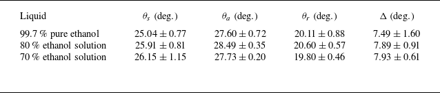
For each kind of liquid, the six maximum values, as shown in figure 5, are averaged as the advancing contact angle $\theta _a$ , while the six minimum values are averaged as the receding contact angle $\theta _r$ . The hysteresis range is then calculated by $\varDelta =\theta _a-\theta _r$ . The static contact angle $\theta _s$ is extracted from the snapshots that record the static free surface and has been averaged with repeated experiments. Measurements of these parameters are listed in table 2. Yang et al. (Reference Yang, Zheng, Luo, Xiao, Li, Luo, Tian, Jiang and Zhao2024) once studied the wettability property of ethanol–water solutions on hydrophobic highly oriented pyrolytic graphite and found that the contact angle decreases with increasing volume percentage of ethanol, consistent with our measured $\theta _s$ .

Table 2.

Contact angle parameters of pure ethanol and its solutions in the PVC container.

Furthermore, meniscus profiles are extracted from experimental snapshots (e.g. figure 4) and compared with numerical results. The static meniscus is obtained directly from the frames without external vibration. The maximum oscillatory displacement is then calculated by subtracting this static profile from the extreme meniscus position observed during vibration. Recalling that the equations governing the static meniscus (3.7b ) and the $\epsilon ^0$ -order problem in § 3.3.1 are solved numerically, using the experimentally measured contact angle parameters in table 2, we obtain the numerical results of $\eta _s'$ and $\check {\eta }_{p1}'$ . In figure 6(a), the theory developed for the static meniscus shows good agreement with experiments, particularly for the lower part. The heights of the menisci are nearly identical, which verifies the measured $\theta _s$ . In figure 6(b), results of $\check {\eta }_{p1}'$ are normalised by setting $\check {\eta }_{p1}'(0)=1$ . The shape of the oscillatory meniscus is basically captured by the theory, except for the region near the lateral walls. At order $\epsilon ^0$ , the free-edge boundary condition (3.9) is imposed on the free surface, implying a shape always orthogonal to the wall, which is absent in experiments.

Figure 6.

Comparison of meniscus dynamics for three working liquids: experimental observations (chain lines) versus numerical solutions (solid lines). (a) Static meniscus profiles $\eta _s'$ and (b) $\epsilon ^0$ -order results of $\check {\eta }_{p1}'$ , normalised by imposing that $\check {\eta }_{p1}' (0 )=1$ .

Figure 7.

Schematic illustration of the experimental set-up for Faraday instability experiments, with the camera focused on the free surface from a front view of the Hele-Shaw cell.

4.2. Faraday onset

In Faraday instability experiments, traditional rectangular Hele-Shaw cells are utilised (see figure 7 for the sketch), with a length of 300 mm and a height of 60 mm. Two different gap sizes are adopted, one of 2 mm and the other of 4.8 mm. The camera is placed perpendicular to the lateral wall of the cell, hence only the Faraday wave profile is observed. We concentrate on the critical acceleration amplitude $a_c$ and the critical wavenumber $k_c$ of linear instability of the free surface. Following the experimental procedure of Douady & Fauve (Reference Douady and Fauve1988) and Li et al. (Reference Li, Li and Liao2019a ), we gradually increase the external acceleration amplitude $a$ by a step of 0.1 $\mathrm{m\,s^{-2}}$ with a fixed driving frequency $f$ . At each level of acceleration amplitude, we wait for 1000 periods of the waves, which is regarded as the growth time for the onset. When Faraday waves emerge, the acceleration amplitude is recorded as the threshold $a_c$ , and the corresponding wavenumber is measured as the critical wavenumber $k_c=2\pi /L_c$ , with $L_c$ denoting the critical wavelength of Faraday waves. Each experiment is repeated three times.

Typically, the threshold measured by gradually raising the driving acceleration corresponds to the lowest point of the Faraday instability tongue (e.g. figure 10), which is, in fact, a tricritical point. Beyond this point, the emerging Faraday waves may be supercritical or subcritical depending on which side of the tongue is considered. The supercritical branch exhibits a continuous smooth instability with a single reversible threshold, whereas the subcritical branch shows hysteresis, with the onset acceleration exceeding the extinction acceleration. Such a bifurcation behaviour of Faraday waves has been well investigated by Rajchenbach & Clamond (Reference Rajchenbach and Clamond2015). However, in their derivation the dynamics of contact angle was not considered. In fact, for our cases, the wetting conditions on the lateral walls from rest to onset and the reverse are different. The contact angle hysteresis maters before the contact line is moving. Once the instability is triggered, the resulting wave amplitude is much higher than that in wide-mouth containers and, most importantly, a liquid film forms on the lateral walls, which was observed both by Li et al. (Reference Li, Li and Liao2019a ) and in our experiments. When such a film is present, there is no longer a sharp contact line between the liquid and the wall. Even if the acceleration is reduced from a fully developed Faraday wave stage, no clear hysteresis effect exists in the wetting dynamics, and the friction force near the lateral wall is significantly diminished, implying that the hysteresis model is not applicable anymore. Given this, when the acceleration decreases from the instability to the still state the model is apparently different from the one used for the emerging process. Therefore, we hypothesise that the supercritical branch could vanish for Faraday instability in Hele-Shaw cells.

Figure 8.

Temporal evolution of the experimentally observed meniscus bottom (black solid line), along with a signal decomposition via fast Fourier transform that extracts the harmonic meniscus wave $\eta '(t')|_{y'=0}$ (red chain line) and the rising subharmonic Faraday wave $\bar {\zeta }'(t')$ (blue dashed line). Results show the data for $80\,\%$ ethanol solution in a cell with $b=2\ \mathrm{mm}$ , measured at a driving frequency of $f=20\ \mathrm{Hz}$ .

The oscillation amplitude of the meniscus wave $| B' |$ is measured by the experimental set-up used in this section. From experimental snapshots in Faraday instability experiments (e.g. figure 7), the free surface is recorded by a distinct black band with a specific width. The upper edge of this band corresponds to the contact line between the liquid and the lateral walls, while the lower edge corresponds to the bottom of the meniscus, implying that the width of the black band reflects the height of the meniscus. The temporal evolution of the bottom of the meniscus is therefore tracked by monitoring the motion of the lower edge of the black band. Since the linear stability analysis targets the critical condition for Faraday onset, corresponding to the moment when the free surface begins to oscillate subharmonically and the contact line starts to move slightly, $| B' |$ should be measured when $a=a_c$ . An example of the experimental evolution of the meniscus bottom is plotted in figure 8. Before onset, the meniscus oscillates harmonically in response to the forcing (confirmed by figure 5), while no visible wave deformation is observed in the $x'$ -direction. Near the onset, the free surface oscillation amplitude grows gradually as the Faraday instability begins to form, as shown in figure 8. This observation interval corresponds to the earliest stage of Faraday instability: the recorded free surface displacement remains below approximately 0.5 mm, which is much smaller than the amplitude of the fully developed Faraday waves ( $\sim$ 10 mm), and is hence consistent with the regime of our study where the Faraday onset is just beginning to emerge. The step-like envelope shown in figure 8 is an artefact of measurement uncertainty, mainly resulting from the finite resolution of the imaging system. According to (2.1), the observed free surface evolution should reflect a superposition of the harmonic meniscus wave and the subharmonic Faraday wave. After a signal decomposition of the experimental data in figure 8 via fast Fourier transform, the amplitude spectrum exhibits two distinct peaks: one at the harmonic frequency (20 Hz, the driving frequency) and the other at the subharmonic frequency (10 Hz), supporting the decomposition treatment adopted for the three-dimensional free surface and the assumed temporal dependence in the ansatzes for both Faraday and meniscus waves. The separated signals are also presented in figure 8, revealing that the amplitude of the nearly invisible ‘Faraday waves’ grows slowly and exponentially while the amplitude of the meniscus wave remains almost constant. 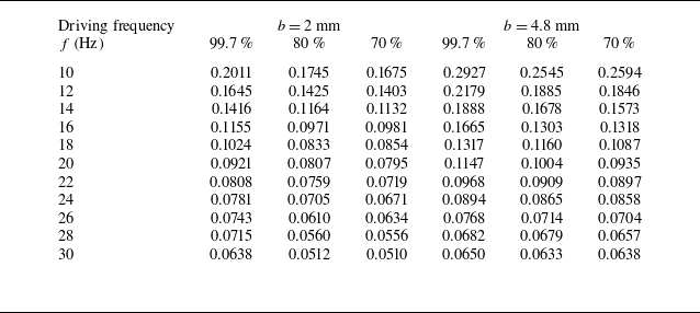The meniscus wave amplitude in each cycle is extracted and averaged to obtain the measurements of $| B' |$ , with three repeated experiments. The resulting values of $| B' |$ for different working liquids and gap sizes, obtained across all experimental driving frequencies, are summarised in table 3.

Table 3.

Experimental results of the real oscillation amplitude of the meniscus $| B' |$ measured in mm. The measurement error is approximately $\pm 0.0071$ mm, primarily resulting from the resolution of the imaging system.

In the present theory, the Hele-Shaw cell is assumed to be infinite in length, which results in the periodic condition in the $x'$ -direction. However, the presence of two ends in the longitudinal direction may influence the results of linear stability analysis. Bongarzone et al. (Reference Bongarzone, Jouron, Viola and Gallaire2023) once employed a thin annulus container to eliminate the effect of two ends. But they imposed that the azimuthal wavenumber is always an integer. Hence, these experiments are limited for identifying the change of $a_c$ and $k_c$ induced by the ends of the cell. Here, we employ a shorter Hele-Shaw cell, which has a length of 100 mm. In this case, the container is not so long compared with the wavelength, and the influence of the ends is more significant. As shown in figure 9(a), for different cell lengths, the critical acceleration $a_c$ is generally consistent, except for the case of $f=14$ Hz. At this driving frequency, the experimental wavelength $L_c$ is not small relative to the cell length $L$ , and $L$ is closest to an integer multiple of $L_c$ ( $L\approx 2.85 L_c$ ). This unique length-scale relationship, absent at other frequencies, may explain the observed discrepancy between different $L$ at $f=14$ Hz. When the cell length is increased to 300 mm, the impact of the ends can be basically ignored. A more detailed examination of this phenomenon lies outside the scope of this work. When it comes to the critical wavenumber, from figure 9(b), we can conclude that the ends of the cell do not affect the dispersion relation at all. Based on the comparisons of $a_c$ and $k_c$ between two different cell lengths, the use of containers with a length of 300 mm guarantees that the Hele-Shaw cell is sufficiently long to make the effect of the two ends negligible when modelling the Faraday instability problem.

Figure 9.

(a) Comparison of the experimental results on $a_c$ for different cell length $L$ . Three different ethanol solutions are used, and $b=2$ mm. (b) Comparison of the experimental results on $k_c$ for different $L$ . The working liquids and gap size are consistent with those in (a). (c) Comparison of the experimental results on $a_c$ for different materials of the Hele-Shaw cell. Pure ethanol is used as the working liquid, and $b=2$ mm.

As we have emphasised before, contact angle hysteresis damping plays an important role in the threshold of Faraday instability and is related to the static contact angle and hysteresis range. These parameters depend on both the liquid (Yang et al. Reference Yang, Zheng, Luo, Xiao, Li, Luo, Tian, Jiang and Zhao2024) and the solid substrate (Shen et al. Reference Shen, Lee, Li, Zaleski, Amberg and Shiomi2024). If we change the material of the Hele-Shaw cell, the contact angle parameters will naturally change, leading to the variation of $a_c$ . This may give intuitive evidence of the impact of dynamic wetting on Faraday waves. Therefore, we conduct experiments in Hele-Shaw cells made of different materials, one of PVC and the other of polycarbonate (PC). As shown in figure 9(c), with only the material changing, the values of $a_c$ are different. This discrepancy cannot be attributed to viscosity or gap-averaged damping, and indicates the significance of contact angle on the Faraday instability problem in Hele-Shaw cells. The comparison also reflects the limitation of the widely used Hamraoui model (1.2) by Li et al. (Reference Li, Li and Liao2019a ), Bongarzone et al. (Reference Bongarzone, Jouron, Viola and Gallaire2023) and Li & Li (Reference Li and Li2024), in which the friction coefficient $\beta$ is only determined by the liquid (Hamraoui et al. Reference Hamraoui, Thuresson, Nylander and Yaminsky2000). This dynamic contact angle model cannot explain the discrepancy in figure 9(c). In addition, noting that $\beta =0.04\ \mathrm{Pa\ s}$ for pure ethanol is obtained using glass capillaries as elucidated by Hamraoui et al. (Reference Hamraoui, Thuresson, Nylander and Yaminsky2000), it is not rigorous to directly apply the experimental measurements of $\beta$ in glass containers to the contact angle dynamics in PVC containers. These wetting parameters must be experimentally measured using containers made of identical materials to those employed in Faraday instability experiments.