


1. Notation
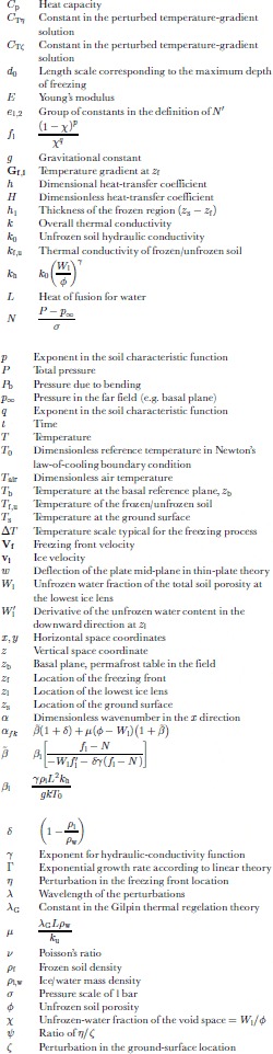
2. Introduction
Frost heave refers to the uplifting of the ground surface owing to freezing of water within the soil. Its typical magnitude exceeds that owing to the mere expansion of water upon freezing (∼9%)because of freezing additional water drawn upward from the unfrozen soil below the freezing front. The process of drawing water through a soil matrix towards a freezing domain is known as cryostatic suction. Primary frost heave is characterized by a sharp interface between a frozen region and an unfrozen region. In contrast, secondary frost heave (SFH) is characterized by a thin, partially frozen region separating the completely frozen region from the unfrozen region. Within this region, termed the frozen fringe, discrete ice lenses can form if there is sufficient ice present to support the overburden pressure. The theory of primary frost heave cannot account for the formation of multiple, discrete ice lenses. Reference Miller and HillelMiller (1980) states that ice-lens formation probably only occurs by the primary heave mechanism in highly colloidal soils with negligible soil particle-to-particle contact.
Frost heave that is laterally non-uniform is referred to as differential frost heave. Differential frost heave (DFH) requires that the freezing be both significant and slow. Adequate upward water flow by cryostatic suction requires either saturated soil conditions or a very high water table because unsaturated soil conditions can suppress the heaving process. Suppression occurs due to insufficient interstitial ice, which is required to support the overburden pressure and allow for ice-lens formation (Reference MillerMiller, 1977).
The DFH process is not fully understood. The complex interactions that occur in freezing soil have not been fully determined or described and there are as yet no predictive models for this phenomenon. However, secondary frost heave, which is often associated with DFH, has received a certain amount of attention from the scientific community. Several mathematical models and empirical correlations have been developed to describe one-dimensional SFH. Most of the mathematical models represent variations and refinements of the original one-dimensional SFH model of Reference O’Neill and MillerO’Neill and Miller (1985). A set of describing equations for three-dimensional SFH based on the O’Neill and Miller model has been developed by Reference Fowler and KrantzFowler and Krantz (1994). Here these equations are used as a basis for investigating the DFH process.
DFH has been cited as a possible cause for some forms of patterned ground by Reference TaberTaber (1929) and Reference WashburnWashburn (1980) among others. Patterned ground refers to surface features made prominent by the segregation of stones, ordered variations in ground cover or color, or regular topography. Since patterned ground is a manifestation of self-organization in nature, its formation is a question of fundamental significance. In this paper, we present a mathematical model for a mechanism by which DFH can occur and may cause the initiation of some types of patterned ground. Using this model, a limited parameter space of environmental (i.e. temperature, snow cover) and physical (i.e. soil porosity, hydraulic conductivity) conditions is defined within which DFH can initiate spontaneously.
3. Prior Studies
Semi-empirical models correlate observable characteristics of the SFH process with the relevant soil properties and climatic variables. The more prevalent models include the segregation potential (SP) model of Reference Konrad and MorgensternKonrad and Morgenstern (1980, Reference Konrad and Morgenstern1981, Reference Konrad and Morgenstern1982) and that of Reference Xiaobai and WangChen and Wang (1991). Typically, semi-empirical models are calibrated at a limited number of sites under unique conditions. Since these unique conditions are accounted for by using empirical constants, it can be difficult to generalize the models for use with varying environmental conditions and field sites. Semi-empirical models are easy to use, computationally simple, and provide fairly accurate predictions of SFH (Reference Hayhoe and BalchinHayhoe and Balchin, 1990; Reference Konrad, Shen and LadetKonrad and others, 1998). However, they provide limited insight into the underlying physics and cannot predict DFH.
Fully predictive models are derived from the fundamental transport and thermodynamic equations. In theory, they require only soil properties and boundary conditions in order to be solved. Based on ideas due to Reference GilpinGilpin (1980) and Reference HopkeHopke (1980), Reference MillerMiller (1977, Reference Miller1978) proposed a detailed model for SFH. This model was later simplified by Reference FowlerFowler (1989), extended to include DFH by Reference Fowler and KrantzFowler and Krantz (1994) and extended further to include the effects of solutes and compressible soils by Reference NoonNoon (1996). Reference NakanoNakano (1990, Reference Nakano1999) introduced a model called M 1 for frost heave using a similar approach. Fully predictive models do not require calibration and can be applied to anywhere the relevant soil properties and thermal conditions are known.These models also provide insight into the underlying physics involved. These attributes facilitate model improvements and extensions. Due to the complexity of some models, they can be computationally difficult and inconvenient to use.
Except under asymptotic conditions, these models must be solved numerically. One-dimensional, numerical solutions to the model by Reference MillerMiller (1977,Reference Miller1978) have been presented by Reference O’Neill and MillerO’Neill and Miller (1982, Reference O’Neill and Miller1985), Reference Black, Miller, Anderson and WilliamsBlack and Miller (1985), Reference Fowler and NoonFowler and Noon (1993), Reference BlackBlack (1995) and Reference Krantz and AdamsKrantz and Adams (1996). In several instances, numerical results agree favorably with laboratory results such as those of Reference KonradKonrad (1989). The predictive capability of the M 1 model has also been demonstrated (Reference Nakano and TakedaNakano and Takeda, 1991, Reference Nakano and Takeda1994).
Reference LewisLewis (1993) and Reference Lewis, Krantz, Caine and ChengLewis and others (1993) were the first to use a linear stability analysis (LSA) in an attempt to predict the occurrence of DFH. Using the model equations developed by Reference Fowler and KrantzFowler and Krantz (1994), they found that DFH occurs spontaneously under a wide range of environmental conditions. Reference LewisLewis (1993) included the necessary rheology by modeling the frozen region as an elastic material and using thin-plate theory. However, this “elastic condition” was incorrectly integrated into the analysis, giving unconventional results that predicted a single unstable wavenumber.
Independently, Reference NoonNoon (1996) and Reference Fowler, Noon and KnutssonFowler and Noon (1997) reported results for a LSA using the Fowler and Krantz model with a purely viscous rheology. Noon’s results indicated that one-dimensional heave is linearly unstable using two different ground-surface temperature conditions: constant temperature and snow cover. However, the constant-temperature results are not physical due to unrealistic parameter choices. The remaining condition necessary for instability, the presence of snow cover, appears too restrictive. Patterned ground is observed both in the presence and in the absence of snow cover (Reference Williams and SmithWilliams and Smith, 1989). Furthermore, since only a single soil was investigated, the influence of soil type on the predictions is difficult to evaluate. In light of these points, further investigation of the linear stability of DFH (this study) was warranted.
4. The DFH Model
The model for SFH that we use in this paper is that due to Reference Fowler and KrantzFowler and Krantz (1994), which is a modified version of the O’Neill and Miller model.We chose to use this model because it contains all the necessary physics to describe DFH while maintaining a numerically tractable form (Reference Fowler and NoonFowler and Noon, 1993). Most importantly, this model properly takes into account thermal regelation in the partially frozen region termed the frozen fringe. Thermal regelation within the fringe allows for differential heaving. The original Reference O’Neill and MillerO’Neill and Miller (1982, Reference O’Neill and Miller1985) model used a rigid-ice approximation that assumes all the ice within the frozen fringe and lowest ice lens moves as a uniform body with a constant velocity. In order for differential heave to occur, this cannot be the case. Reference Fowler and KrantzFowler and Krantz (1994) demonstrate that thermal regelation within the fringe allows for DFH. Readers should refer to Reference Fowler and KrantzFowler and Krantz (1994) and Reference Krantz and AdamsKrantz and Adams (1996) for details.
4.1. Physical description
The physical system in which frost heaving occurs is shown in Figure 1. Top-down freezing occurs over a time-scale of weeks to months. The upper, frozen region is separated from the lower, unfrozen region by the frozen fringe, a partially frozen transition region containing ice, liquid water and soil. The thickness of the frozen fringe in seasonally frozen ground is on the order of 1–10 mm. The frozen region is characterized by regular bands of pure ice called ice lenses. It is the existence of ice lenses that gives rise to surface heave greater than the 9% associated with the volume change of water upon freezing (Reference WashburnWashburn, 1980). In typical field situations where frost heave occurs, permafrost underlies the unfrozen region (Reference Williams and SmithWilliams and Smith, 1989).
Diagram of saturated soil undergoing top-down freezing. The region between zl and zf is the frozen fringe. Ice lenses occur in the frozen region, giving rise to frost heave.

Because the frozen fringe is relatively thin, it can be reduced mathematically to a plane across which jump boundary conditions are applied (Reference Fowler and KrantzFowler and Krantz, 1994). This plane is located at z
f in Figure 1. Freezing of saturated soils is fairly slow, as can be inferred from the large Stefan number  associated with this process. Because the time-scale for freezing is much longer than that for heat conduction, the temperature distributions in the unfrozen and frozen regions are quasi-steady state. The thermal gradients in the unfrozen and frozen region are obtained by solving for the temperature distributions in each region.
Because ice lenses occur in a discrete manner, the frost-heave process is inherently a discontinuous process. However, Reference Fowler and KrantzFowler and Krantz (1994) demonstrate using scaling arguments that the time-scales for equilibration of the pressure and temperature profiles within the frozen fringe are much shorter than the time-scale for the freezing process. Thus, the entire frost-heave process can be modeled as semi-continuous where some parameters are evaluated at the base of the warmest (lowest) ice lens, z l.
For one-dimensional frost heave, the surfaces z s and z f are parallel planes. The frozen region including ice lenses moves upwards relative to z b but does not deform. In this instance, the rheology of the frozen material is irrelevant. In DFH, however the frozen region deforms as it moves, and the rheology of the material must be specified so the mechanical problem can be solved in conjunction with the thermal and frost-heave problems.
4.2. Thermal problem
Due to the large Stefan number for freezing soil, the thermal problems in both the frozen and unfrozen regions above and below the frozen fringe, respectively, are greatly simplified. The two-dimensional, steady-state temperature distributions in both regions are obtained from the solution to the Laplace equation:


The boundary condition at the ground surface is Newton’s law of cooling. For both problems, the boundary condition at z f specifies the temperature as the standard temperature and pressure (STP) freezing point of water. For this paper, the temperature at z b will also be specified.


where H is a heat-transfer coefficient, T air is the dimensionless air temperature at the ground surface and T b is the dimensionless temperature of the underlying permafrost. In the absence of significant solutes, T b = 0, corresponding to 0°C.
4.3. Mechanical problem
The choice of an elastic rheology can introduce several conceptual and modeling difficulties. To address these difficulties, we adopt several assumptions about the geometry of the frozen region as well as its mechanical properties. The frozen fringe is, mathematically, reduced to a plane across which jump boundary conditions are applied (Reference Fowler and KrantzFowler and Krantz, 1994). This plane is the lower boundary of the frozen region, z f . However, because it will be perturbed and distorted, albeit infinitesimally, and will no longer be a plane in a strict mathematical context, we refer to it as an interface.
Figure 2 shows a schematic of the frozen fringe before and after inception of DFH due to initiation of a new ice lens. In fact, the location of the newly forming ice lens is very close to the base of the lowest ice lens relative to the thickness of the frozen fringe. There is a boundary layer in the frozen fringe near the lowest ice lens wherein most of the pressure drop causing upward permeation occurs. The new ice lens will form within this boundary layer (Reference Fowler and KrantzFowler and Krantz, 1994).
Diagram of the frozen fringe showing the initiation of DFH. Relative dimensions are not to scale.The dashed line in the left figure shows the location of zf which is defined where the ice content is zero. A new ice lens forms within the water-pressure boundary layer below the lowest ice lens. After initiation of a new ice lens, the location of zf will move either upwards or downwards relative to its previous position. The two possibilities are shown by  and
 .The ice crystals labeled “possible ice” will exist for
 and not for
 .The new location of zf is predicted by the LSA and is not prescribed in the model.

The dashed line labeled z f is the bottom of the frozen fringe, defined as where the ice content is zero. At the inception of DFH, the location of z f can move either up or down. Because of the quasi-steady-state assumption, any movement of z f is relative to the stationary, one-dimensional boundary. Although z f is always moving downwards on the time-scale of freezing-front penetration, quasi-steady state must be assumed in order to conduct the LSA. While this is an abstraction from reality, it is an expedient and useful practice for LSA of systems with unsteady basic states (Reference FowlerFowler, 1997). Two possible locations for z f are shown in Figure 2 (right side): one for upward movement and one for downward movement. Which of these two possible outcomes actually occurs is not prescribed in the model but is a result of the LSA. However, linear theory does prescribe that z f is either in phase or anti-phase with the ground-surface perturbation, z s. Any relative displacement other than 0 or π is not allowed. The location of z l in Figure 2 will be in phase with the ground surface at z s since the lowest ice lens precludes water migration above it. Thus, Figure 2 demonstrates how z s and z f can be either in phase or anti-phase due to the formation of a new ice lens.
Mechanically, when non-uniform ice-lens formation begins, the frozen region will begin to deform and bend. We model this as the bending of a thin, elastic plate, though a viscous, viscoelastic or visco-plastic model might also be used. Laboratory experiments by Reference TystovichTsytovich (1975) demonstrate that frozen soil does behave elastically on short time-scales. The necessity for including the rheology of the frozen material in the model is to provide a “resistive force” to deformation of the frozen material. As will be demonstrated later, when the rheology is neglected, a LSA predicts that the most unstable mode has a wavelength approaching zero, which is intuitively incorrect.
A conceptual difficulty is encountered when assuming an elastic rheology in this problem since frozen material is being accreted. This problem can be avoided if we neglect the addition of newly frozen material in the geometry of the elastic material being bent. What this means physically is that when a non-uniform ice lens begins to form, only the material spanning from the ground surface, z s to the lowest ice lens, z l, is actually being bent. In the sense of the elastic model, the newly accreted material has an elastic modulus of zero. This approach is convenient because it avoids some inherent complexity, and there is considerable justification for its use. Experimental data for Young’s modulus of frozen soil as a function of temperature show that the modulus approaches zero as the sub-freezing temperature approaches zero (Reference TystovichTsytovich, 1975, p.185). Large amounts of unfrozen water at 0°C are the cause of this “weakness”. Thus, we would expect the newly accreted material to have a very low Young’s modulus, so that neglecting it completely introduces only a small error. In fact, as a first approximation the entire frozen region is assumed to have a constant Young’s modulus. This approximation is crude since there is a non-zero temperature gradient within the frozen region. In reality, the Young’s modulus monotonically increases with decreasing temperature and has a maximum value at the ground surface where it is coldest.
Due to the simplifications discussed above, the mechanical model reduces to the bending of a thin, elastic plate with a constant Young’s modulus. If the deformation is small relative to the thickness of the plate, the deflection of the plate’s mid-plane from equilibrium, w, can be approximated as (Reference Brush and AlmrothBrush and Almroth, 1975):


where P b is the pressure, E is Young’s modulus, h 1 is the frozen-region thickness and ν is Poisson’s ratio. In this analysis, ν = 0.5.
Boundary conditions for Equation (7) must be specified in the x and y directions. Because the problem is unbounded in these directions, periodic boundary conditions are used. For the x direction,


There is a corresponding set for the y direction (however, only the two-dimensional problem will be considered here). The mechanical problem is coupled to the frost-heave problem through the load pressure at z l. In the one-dimensional basic state, the frozen region is planar and there is no bending (P b = 0). In the two-dimensional state, the non-zero P b is a function of x. The load pressure is the sum of the weight of the overlying soil and the pressure due to bending.

4.4. Non-dimensionalized frost-heave equations
The Fowler and Krantz frost-heave equations are two coupled vector equations that describe the velocity of both the upward-moving ice at the top of the lowest ice lens, vi , and the downward-moving freezing front, Vf . Specifically, the equations are:


where Gi and Gf are the thermal gradients in the unfrozen and frozen regions, respectively, φ is the soil porosity, W l is the unfrozen-water volume fraction at the top of the frozen fringe (base of the lowest ice lens), and k f and k u are the frozen and unfrozen thermal conductivities, respectively. Vectors are denoted in bold, and the coordinate system is oriented with z pointing up as shown in Figure 1. The value of W l is determined using the lens-initiation criterion (Reference Fowler and KrantzFowler and Krantz, 1994) that involves the characteristic function.

The solution to the one-dimensional problem is fairly straightforward.The steady-state, one-dimensional Laplace equation for temperature is solved to determine the relevant temperature gradients Gi and Gf . Work by Reference Fowler and NoonFowler and Noon (1993) and Reference Krantz and AdamsKrantz and Adams (1996) has shown that this model predicts the one-dimensional frost-heave behavior observed in the laboratory quite well.
5. Linear Stability Analysis
LSA is performed here to determine under what circumstances the one-dimensional solution to the SFH equations (15) and (16) is unstable to infinitesimal perturbations. The conditions under which the one-dimensional solution is unstable will provide insight into the mechanisms responsible for DFH. This in turn will help explain the evolution of some types of patterned ground that are due to DFH.
The LSA performed here follows standard linear stability theory (Drazin and Reid, 1981). A complete detailed analysis is available in Reference PetersonPeterson (1999). Equations (15) and (16) are perturbed around the one-dimensional basic state solution and linearized. Because the equations are linear in the perturbed variables, the solution to these perturbed variables will take the general form:

where α and β are the wavenumbers of the disturbance in the x and y directions, respectively. Because one-dimensional frost heave occurs in the z direction, perturbations in both the x and y directions cause a three-dimensional shape to evolve. Initially, however, only the propensity for a two-dimensional instability will be investigated by setting β = 0. The functional form of  in Equation (18) depends on whether the problem is steady-state or transient. Although the frost-heave process is inherently transient, it will be treated as quasi-steady-state. If the instabilities grow very rapidly relative to the basic state, this assumption is justified. A successful example using this technique for alloy solidification is presented in Reference FowlerFowler (1997). In this instance, assuming quasi-steady state yields results somewhat close to experimental observations. Thus, the solution to the perturbed variables takes the general form:

where Γ is an exponential growth coefficient.
The perturbed temperature distribution is determined in terms of the basic-state temperature distribution. First, the solution to Equation (2) subject to boundary conditions (3) and (4) yields the unperturbed temperature in the frozen region:

Solution of Equation (1) subject to boundary conditions (5) and (6) is trivial when T b = 0.

The frost-heave equations (15) and (16) require the thermal gradient at z f. Steady state is also assumed in the perturbed region in anticipation that the time-scale for perturbation growth is greater than the time-scale for heat conduction. Starting with the two-dimensional form of Equation (2), the temperature is perturbed and the differentiation carried out. Boundary conditions are applied at perturbed locations, where the Taylor series is truncated after the linear term. The perturbed temperature field is solved and then differentiated again to yield:

Where


The thermal gradient below the freezing front is assumed to be zero in this analysis. This condition is representative of active-layer freezing above permafrost. Thus,  .
The perturbed mechanical problem begins by perturbing the pressure condition, Equation (14). The pressure is non-dimensionalized with the pressure scale σ.

The linearized form of N′ is:

where


 is the thickness of the frozen region and E is Young’s modulus.
The frost-heave equations (16) and (15) are complicated functions of the temperature gradients and the pressure at the top of the frozen fringe. Each potentially varying parameter must be perturbed (e.g. replacin  with
 ). Thus, the following parameters are perturbed: β, f
l, G
i, G
f, N, V
f, v
i, W
l, z
f and z
s.
The perturbed variables are substituted into Equations (15) and (16), and the equations linearized. Two equations result that describe the perturbed ice and freezing-front velocities in terms of perturbed quantities:

and

The perturbed temperature gradients and pressure were determined in the previous sections. The remaining perturbed variables can be cast in terms of N′ by use of their definitions. Then using Equation (26), the two equations are only functions of η and ±. This process is straightforward but algebraically complicated (Reference PetersonPeterson, 1999).
The perturbed velocities are determined using the kinematic condition. The kinematic condition at the freezing front is slightly complicated because the flux of material through the boundary z f must be accounted for. However, because the accreted material is neglected in the elastic model, both conditions are straightforward:


Solution of the perturbed frost-heave equation is now possible. Equations (29) and (30) can be expressed in terms of Γ, α, η, ζ and parameters that are constant for the specific case being analyzed. An eigenvalue problem for the growth coefficient Γ as a function of α results.

The algebraically cumbersome expressions for A, B and C can be seen in Reference PetersonPeterson (1999). An explicit expression for the two roots of Γ is easily obtained.
6. Linearized Model Predictions
This section presents the predictions obtained from the LSA. It was shown in section 4 that there are many parameters that arise from the frost-heave model. These are divided into three groups: soil parameters, environmental conditions and physical constants. We define a reference set that comprises a set of environmental conditions about which we will vary some parameters and analyze their effect on the stability of one-dimensional frost heave. These conditions were chosen to be representative of areas where DFH is observed. There are an additional six parameters that describe the particular soil being analyzed: p, q, φ, k 0, γ and ρ s. The first two come from the characteristic function that relates the difference in ice and water pressures to the amount of unfrozen water. The values of p and q are determined empirically by fitting the characteristic function to experimental data. In this paper, three different types of frost-susceptible soils are analyzed: Chena Silt, Illite Clay and Calgary Silt. These soils were chosen because values for all six parameters could be obtained from previously published data (Reference Horiguchi and MillerHoriguchi and Miller, 1983) with curve fitting when necessary. Table 1 lists the values for all six soil parameters for the three soils investigated.
Parameter values for frost-susceptible soils

The environmental conditions include the temperature boundary conditions at the ground surface, z s, and at the permafrost table, z b. The general Newton’s law-of-cooling boundary condition is applied at the ground surface. The effects of varying degrees of snow cover (including none) and differing vegetative cover can be explored using this boundary condition. For simplicity, the gradient in the lower, unfrozen region is zero for this analysis.
The final environmental condition is the freezing depth, h 1. This parameter has a range in dimensional form of 0 → d 0, where d 0 is the depth of the active layer. It should be apparent that the freezing depth is a function of time. As freezing progresses, h 1 increases. Thus, by specifying a value for h 1 in the reference set of parameters, the stability of one-dimensional frost heave at a certain, frozen instant of time is being analyzed. The value of h 1 for the reference set was chosen to correspond to a time early in the freezing process, when it is believed DFH is most likely to be initiated. It will be shown in section 6.7 that the mechanism for instability is related to differential heat transfer. The temperature gradient in the frozen region is greatest early in the ground-freezing process, so DFH is more likely to initiate at early times in the freezing process. The quasi-steady-state assumption allows for specification of h 1.
The physical constants that arise in this problem are primarily concerned with the properties of ice and liquid water. These values are summarized in Table 2. A constant-temperature boundary condition of −10°C was chosen for the top surface (Reference SmithSmith, 1985). This is accomplished in the thermal problem by allowing H → ∞. Chena Silt was chosen as the soil type because, as will be demonstrated, it has the greatest range of unstable behavior. A depth of freezing of 10 cm, or about 10% of the maximum depth of freezing, was also chosen. There is no surface load because in field situations the only overburden is the weight of the frozen soil. A Young’s modulus of 5 MPa is used for the elastic modulus (Reference Andersland and LadanyiAndersland and Ladanyi, 1994).
Physical constants for the LSA model

6.1. Effects of parameter variations
In the following subsections, the effects of varying different parameters from their reference-set values are investigated. The results are presented by plotting the dimensionless growth rate, Γ, as a function of the dimensionless wavenumber, α (see Equation (19)). The scaling factors for these parameters are


For comparison purposes, the results will be presented in dimensionless form. The stability criterion, Equation (33), is quadratic, and therefore there are two roots Γ+, Γ−, with Γ+ > Γ−. In this analysis, the lower root Γ− was always negative. The positive value, Γ+, is plotted for the reference set using Chena Silt in Figure 3. In all cases, both roots are real numbers for the range of α values presented, and the principle of exchange of stabilities is valid (Reference Drazin and ReidDrazin and Reid, 1991).
Plot of the positive root of the linear stability relation as a function of the wavenumber for the reference set of parameter values.The soil is Chena Silt.Wavenumbers greater than αntl are stable and αmax is the wavenumber with the maximum growth rate under these conditions.

There are three values that are of most importance in each plot: Γmax, α max and α ntl, indicated in Figure 3. The maximum value of the growth rate, Γmax, and the corresponding value of the wavenumber, α max, indicate which mode grows fastest in the linearized model. Also, α max indicates the lateral spacing of the most highly amplified, two-dimensional mode through Equation (35). The neutrally stable wavenumber, α ntl, indicates the maximum wavenumber for which modes can be linearly unstable. These values are not explicitly marked in subsequent figures, to reduce clutter.
6.2. Effect of soil type
The type of soil is the most influential parameter in the model when determining the stability of one-dimensional frost heave. It is important to note that only a small fraction of soils exhibit frost heave (Reference Williams and SmithWilliams and Smith, 1989). A delicate balance between the hydraulic conductivity of the partially frozen soil, particle size and its porosity is necessary for frost heave to occur. Silts and silty clays meet these requirements in general. Furthermore, DFH is not necessarily observed in all frost-susceptible soils. Determining whether this observation is due to the specific soil or its environmental conditions is a major objective of this analysis. Figure 4 plots the growth rate as a function of wavenumber for the three soil types specified in Table 1.
The linear growth coefficient for three soil types using the reference set of parameter values.

All three soils are considered frost-susceptible. However, for the reference set of parameter values, only Chena Silt has a propensity for DFH (i.e. positive value of Γ+). It should be noted that these results do not indicate that Calgary Silt and Illite Clay will never heave differentially. Other parameters can have a significant effect on the stability predictions, and under the correct conditions the soils may heave differentially.
The utility of a model such as this one hinges on whether it can predict observations made in the field. Unfortunately, there is a limited number of soil types to analyze due to a dearth of adequate characterization data including hydraulic conductivity and sub-freezing temperature as functions of unfrozen water content. In fact, the work by Reference Horiguchi and MillerHoriguchi and Miller (1983) is one of the few comprehensive datasets for frost-susceptible soils available in the open literature. Fortunately, the predictions shown in Figure 4 do agree with observations made in the field. In almost all instances, hummocks are observed in silty-clayey materials. The value of α max for Chena Silt is of the order unity. This wavenumber corresponds to a dimensional wavelength on the order of meters, which is also observed in the field (Reference Williams and SmithWilliams and Smith, 1989). The value of Γmax is several orders of magnitude less than unity, indicating that DFH will take (dimensionally) several years to develop. It is commonly believed that most types of patterned ground form on the 10–100 year time-scale (Reference MackayMackay, 1980; Reference Hallet, Nicolis and NicolisHallet, 1987).
6.3. Effect of the elastic constant
In this and subsequent subsections, we investigate the effects of parameter variations away from the reference set for Chena Silt, which has the greatest propensity for DFH. Although calculating the effect of the elastic constant on linear stability is not difficult, interpreting the results can be confusing due to some of the assumptions made in the mechanical model. The complication arises due to the difficulty in determining an appropriate value for the Young’s modulus, E. While there are several references that address the Young’s modulus for frozen soils (Reference TystovichTsytovich, 1975; Reference Puswewala and RajapaksePuswewala and Rajapankse, 1993; Reference Andersland and LadanyiAndersland and Landanyi, 1994; Reference Yuanlin, Ping, Jiayi and JianmingYuanlin and others 1998), there is a large range of reported values. Reference Andersland and LadanyiAndersland and Ladanyi (1994) report that for frozen silts, sands and clays, a Young’s modulus of about 5 MPa is typical for the temperature range of interest: −10 → 0°C. The effect of Young’s modulus on the growth-rate predictions is shown in Figure 5.
The linear growth coefficient, Γ+, as a function of wavenumber, α, for three values of the Young’s modulus, E.The soil type is Chena Silt.

As might be expected, the range of unstable modes decreases with increasing Young’s modulus. The value of α max decreases, indicating that a “stiffer” soil results in less closely spaced patterning. Because Γmax decreases with increasing E, it would also take longer for patterns to become expressed in stiffer soils. It appears that increasing elasticity is a stabilizing mechanism. As it becomes more difficult to “bend” the frozen region, the propensity for differential heave is reduced.
It is worth noting that only in the limit of E → ∞ does the propensity for DFH at some value of α disappear. Both α ntl and α max approach zero only when E → ∞. One major cause for larger values of E for a particular soil would be colder temperatures. However, colder temperatures also affect the thermal regime in the frozen region.This effect is explored separately in section 6.4 and 6.5.
6.4. Effect of the ground surface heat-transfer coefficient
In all the previous results, we have assumed a constant temperature of −10°C at the ground surface. However, a constant-temperature condition is unrealistic for prolonged periods of time (i.e. > 1–2 days). A lumped parameter boundary condition with an overall heat-transfer coefficient is more reasonablefor long-term analysis.The constant-temperature condition is obtained from the heat-transfer-coefficient condition by allowing H → ∞. Figure 6 plots Γ+ as a function of α for three values of the dimensionless heat-transfer coefficient. A dimensional value of the heat-transfer coefficient, h, can be obtained by reversing the scaling  .
The linear growth coefficient, Γ+, as a function of wavenumber, α, for three values of the dimensionless heat-transfer coefficient  . The value of Γmax for H = 10 is two orders of magnitude greater than for a constant-temperature boundary condition (H → ∞).

It is readily apparent that the “insulating” effect represented by smaller values of H causes a greater range of unstable modes. Furthermore, as H decreases from ∞ to 10, Γmax increases two orders of magnitude. Insulation obviously has a destabilizing effect.
Both α max and the corresponding value of Γmax increase as H decreases. There are several scenarios in the field in which small values of H might be applicable. The most obvious instance is that of increased ground cover in the form of grasses, mosses and shrubs. It is noteworthy that the extensive survey of earth hummocks byReference Tarnocai and ZoltaiTarnocai and Zoltai (1978) supports this prediction. In essentially all places where earth hummocks are found, there is a moderate amount of organic ground cover. The fact that the tops of hummocks are sometimes more barren than the trough regions is most likely the result of changes in soil moisture after the hummock shape has matured. It is reasonable to assume that the differential height between the crest and the trough would cause water drainage from the top that collects in the inter-hummock spaces, thus propagating further organic growth in the depressions.
6.5. Effect of ground-surface temperature
Snow cover, which is almost always present to some degree in arctic and subarctic regions, also has an insulating effect. However, snow is more likely to maintain a constant temperature at the ground surface due to its ability to function as a “heat sink” because of the relatively large latent heat associated with freezing. To analyze the effect of snow cover, it is more useful to return to the constant-temperature boundary condition and vary the value of T air. Since H → ∞ for the constant-temperature condition, the ground-surface temperature is equivalent to T air. A smaller (in magnitude) value of T air corresponds to a thicker and/or less thermally conductive snow layer. In fact, the only limitation in this case is T air < 0. The effect of the ground-surface temperature is shown in Figure 7.
The effect of warmer constant-temperature conditions on the growth of differential modes for the reference set of parameter values.The growth rate, Γ is plotted in dimensional form.

In Figure 7 it can be observed that as the ground-surface temperature warms, Γmax decreases. Furthermore, in the limit of T air → 0, the growth coefficient for all unstable modes tends to zero. These results indicate that the occurrence of DFH should be more prevalent in less snow-covered areas than those where snow accumulates, and in fact this is observed. A good example is the Toolik Lakes (Alaska, U.S.A.) field site where D. A. Walker (personal communication, 2000) has observed that frost boils tend to be more prevalent in the wind-blown areas. Frost boils are small mounds of soil material, ∼1 m in diameter, presumed to have been formed by frost action (NSIDC, 1998). Ground-surface temperature measurements in both regions confirm that surface temperatures are indeed colder in the barren regions.
6.6. Effect of freezing depth
It is appropriate to investigate the effect of freezing depth, h 1 ≡ z s − z f, on the stability theory predictions.The non-dimensionalization establishes that h 1 is of the order one.When ground freezing commences, h 1 begins at zero and increases (approximately with the square root of time (Reference Fowler and NoonFowler and Noon, 1993)). By examining the behavior of α max and Γmax for increasing values of h 1, we are able to observe how the stability of the system changes as ground freezing progresses. Figure 8 shows the effect of freezing depth on the stability analysis predictions. As one might expect, the largest range of unstable modes occurs at the smallest values of the freezing depth and slowly decreases as h 1 increases. However, contrary to previous results where unstable modes existed for all values of a parameter, stabilization occurs at a finite value of h 1. For the reference set of parameter values shown here, that value is h 1 ≈ 0.23, which corresponds to a dimensional value of 23 cm.
The linear growth coefficient, Γ+, as a function of wavenumber, α, for three depths of freezing, h1.There are no positive roots (Γ+, Γ− <0) at freezing depths greater than h1 ≈ 0.23.

The fact that there is a critical value of the freezing depth is important when attempting to gauge what wave-number might commonly be most expressed in the field. In the limit h 1 → 0, all wavenumbers have a positive growth rate. As freezing progresses and h 1 increases from zero, the largest wavenumbers are “cut off ” (i.e. Γ+ < 0) while the smaller wavenumbers continue to grow, albeit at a slower rate. As h 1 continues to increase, more and more wavenumbers are cut off. Eventually when h 1 ≈ 0.23, all wavenumbers are cut off and no differential modes are unstable. It can be seen in Figure 8 that very small wavenumbers always have small positive growth rates until cut off. Large wavenumbers have large growth rates but are cut off early. Mid-range wavenumbers have moderate growth rates for intermediate periods of time. Thus, mid-range wavenumbers might become most expressed in the field since they have a moderate length of time to grow and moderate growth rates for most of the time.
Although linear theory is not strictly valid once differential modes grow to a finite amplitude, it is insightful to see what wavenumber the model predicts would become most expressed during the entire period of freeze-up. This assumption is not excessively crude since the dimensionless growth rates are much less than unity in this case, and the perturbations are going to grow relatively slowly. As a simple approximation, we define the normalized growth rate as follows:

where ζ is the perturbation in the ground-surface location. The magnitude of ± at time t′ is determined by integration:


where ζ 0 is the magnitude of the original perturbation at t = 0.
Figure 9 shows the numeric results of integrating Equation (38) for several values of the wavenumber α, indicated by the dots. The integration is performed until a time t′, at which point all modes become stable (i.e. h 1 ≈ 0.23). The most expressed wavenumber under these conditions is α = 2.3 which corresponds to a dimensional wavelength of 2.7 m. This result is quite encouraging since the spacing of hummocks is typically 1–3 m (Reference Tarnocai and ZoltaiTarnocai and Zoltai, 1978). Because all modes are stable for times greater than t′ (or h 1 > 0.23), a further increase in frost depth will result in all modes decreasing in amplitude.
Relative amplitude of the ground-surface perturbation, ζ/ζ0, for several values of the wavenumber, α, at the time t′ when all modes become stable. Soil type is Chena Silt and H = 10. At t = t′, h1 ≈ 0.23.

To determine the evolution of ζ/ζ 0 in time as h 1 increases, Equation (38) is integrated in time up to t′ for a given wavenumber. The results for α = 2.6 are shown in Figure 10. This figure shows the evolution of ζ/ζ 0 as freezing progresses (i.e. h 1 increases). The normalized perturbation amplitude reaches a maximum at h 1 ≈ 0.08 and then begins to decrease. At h 1 = 0.2, ζ/ζ 0 ≈ 2.65 as expected from Figure 9. The amplitude returns to its initial value at h 1 ≈ 0.36 and continues to decrease as h 1 increases further. These results indicate that an initial perturbation of magnitude ζ 0 will have increased in magnitude at the end of the freezing season for active-layer depths < 0.36 m.
Evolution of the normalized ground-surface perturbation as a function of the freezing depth, h1.

There is no assumption in this derivation that the perturbation grows as exp[Γ t] as linear theory requires. In this sense, this is a real-time analysis. However, other assumptions have implications that must be examined. Perhaps most importantly, all product terms in perturbed variables are assumed small and neglected. Hence, this real-time analysis is still only applicable when all perturbations are relatively small in magnitude.
6.7. Mechanism for instability
It has been demonstrated above that there is a range of modes that are unstable for most cases of interest. In fact, if the Young’s modulus is allowed to approach zero (E → 0), all modes are unstable for some soils while no modes are unstable for other soils. In this limit, the bending resistance of the frozen soil is essentially removed (see Equation (7)). Figure 11 shows the LSA prediction for the reference set of parameter values and Chena Silt except that E = 0. It is evident that the elasticity of the frozen layer is providing the stabilizing mechanism for DFH.
Stability predictions for the fundamental case when theYoung’s modulus is set to zero (E = 0).

In order to help explain the mechanism that causes the instability, Figure 12 shows a schematic of the in-phase perturbed surfaces. Also sketched are approximate isotherms for the constant-temperature boundary condition at the top surface. The large arrow pointing to the right shows the net direction of differential heat flow that is occurring from a crest region to a trough region. Before the perturbations occur, heat transfer occurs only in the vertical direction. However, once the system is perturbed, heat transfer can occur in both the horizontal and vertical directions.
Schematic of the perturbed surfaces showing isotherms and the direction of differential heat flow.The basic state surfaces  and
 are shown by the dashed lines, and the perturbed surfaces are the thick solid lines.

Solving Equation (33) for η/ζ indicates that the magnitude of the bottom surface perturbation, η, is less than the top surface perturbation, ζ, albeit by a small difference. However, linear stability theory predicts perturbations grow exponentially. Thus, although the difference between η and ζ is small initially, that difference will grow exponentially fast (at least until non-linear terms become significant). In fact, it is difficult to speculate about what form the perturbations will take once non-linear terms become significant. Figure 12 shows that the thickness has increased from the basic state value underneath a crest, and decreased underneath a trough. Because the temperatures at the boundaries z f and z s are fixed at the basic-state values and the conduction path length has changed, the temperature gradient at the bottom surface, Gi, has also changed. Underneath a crest the gradient has decreased in magnitude and, according to Equation (15), the velocity of the freezing front will also decrease. Continuing this line of reasoning, since the conduction path underneath a trough has decreased, the gradient at z f has increased and the velocity of the freezing front has correspondingly increased. Since there is a positive feedback mechanism occurring at this point, the perturbations will continue to grow.
In order to understand the increase in Γ with increasing wavenumber observed in Figure 11, it is necessary to consider the magnitude of differential heat flow shown in Figure 12. As the wavenumber increases, the magnitude of heat flux from a crest region to a trough region increases. In order for frost heave to occur, the latent heat of the incoming water at z l must be removed. Since there is differential flow from a crest to a trough, additional heaving can occur underneath the crest region. This also corresponds to less heave occurring in the trough region.
6.8. Implications of the steady-state assumption
This analysis is based on the quasi-steady-state assumption that perturbations grow much faster than changes in the basic state. However, predictions indicate that the growth rate Γ is actually less than unity in most cases, and thus perturbations grow slowly relative to changes in the basic state. For some time-periodic problems with slow growth rates, Floquet theory has been successfully applied when solving the linear stability problem (Reference Drazin and ReidDrazin and Reid, 1991, p. 354). However, the entire freeze–thaw cycle (or period) must be modeled. This analysis has only addressed the frost-heave process that occurs during freezing, which is only part of a larger cycle. The thawing process involves solifluction, soil consolidation, water percolation and evaporation, and possibly other processes.
The present analysis indicates that the frost-heave process alone is capable of causing spontaneous pattern generation, albeit on a 10–100 year time-scale. Combination of the frost-heave model with a thaw model could possibly yield more conclusive theoretical evidence that patterns are generated by the processes discussed here. It may be that the mature periglacial patterns observed are actually the result of a complex combination of all the processes mentioned above.
7. Conclusions
In this paper, we have demonstrated that the frost-heave model due to Reference Fowler and KrantzFowler and Krantz (1994) is linearly unstable under a range of environmental conditions and for several (but not all) soil types. Differential heat flow coupled with the delicate balance between hydraulic conductivity and cryostatic suction potential act as a destabilizing mechanism for one-dimensional frost heave. When the upper frozen region is modeled as a purely elastic material, the force required to deform the frozen region acts as a stabilizing mechanism to DFH. Previous stability analyses in the literature (Reference Lewis, Krantz, Caine and ChengLewis and others, 1993; Reference Fowler, Noon and KnutssonFowler and Noon, 1997) have failed to describe accurately the mechanisms at work that can give rise to DFH. The analysis presented here has corrected errors in how Reference LewisLewis (1993) coupled the mechanical problem to the frost-heave problem, and identified a source of instability that was overlooked by Reference NoonNoon (1996) in the case of a constant-temperature boundary condition.
The mechanisms responsible for DFH are dependent on the instantaneous depth of freezing and can effectively be shut off when depths of freezing exceed a critical value. Numerical integration of the predicted growth rates as freezing progresses beyond this critical value indicates that there is an intermediate-valued wavenumber that is most expressed.
The dimensionless growth rates predicted by the theory presented here are small, ≪1, indicating that pattern expression would take tens to hundreds of years to mature. This predicted length of time is similar to the scale reported by many field observers (Reference WashburnWashburn, 1980; Reference Williams and SmithWilliams and Smith, 1989). However, the mechanisms discussed here apply only to the freezing process. Active-layer thaw is itself a unique process and may possess additional mechanisms that could give rise to patterning. One possibility is the buoyancy-induced soil circulation theory presented by Reference Hallet, Waddington, Dixon and AbrahamsHallet and Waddington (1992). Coupling the DFH model with Hallet and Waddington’s model might provide a more complete explanation of pattern formation and soil circulation by accounting for both the freezing and thawing processes.
The use of thin-plate theory to describe the upper, frozen region as a purely elastic material is restricted to the linear region. Vertical displacements are assumed very small. Furthermore, thin-plate theory assumes h 1 ≪ 2πλ, or that the thickness of the region being deformed is much less than the characteristic lateral dimension. This assumption is obviously not valid for larger freezing depths. To describe the evolution of DFH after initiation when these assumptions break down, a more comprehensive elastic constitutive relation needs to be implemented. Alternatively, a different rheology can be used such as viscous, viscoelastic or viscoplastic. These rheologies may in fact describe the long-term evolution of DFH more accurately than a purely elastic one.
The steady-state assumption can only be used as a first approximation and is obviously invalid near marginal stability. This drawback points to the necessity of solving the non-linear equations as a time-evolution problem. While a non-linear stability analysis can provide further information about the observed planform and sub- or supercritical stability, it must also use a frozen-time assumption. Current stability theory cannot adequately account for the effects of a changing basic state. Thus, a numerical solution of the time-evolution problem is probably the most valuable continuation of this investigation.
Acknowledgements
We greatly appreciate the helpful comments from S. J. Jones, M. Sturm and an anonymous reviewer. This work was supported by U.S. National Science Foundation grant OPP-9321405. R.A.P. acknowledges the American Geophysical Union for financial support.



