1. Introduction
The phenomenon of turbulent thermal convection occurs widely in both natural and industrial processes. Rayleigh–Bénard convection (RBC), which comprises a fluid layer that is heated below and cooled above, is a simple but classical model of thermal convection that has been studied extensively over several decades (for reviews, see Siggia Reference Siggia1994; Kadanoff Reference Kadanoff2001; Ahlers Reference Ahlers2009; Ahlers, Grossmann & Lohse Reference Ahlers, Grossmann and Lohse2009; Lohse & Xia Reference Lohse and Xia2010; Chillà & Schumacher Reference Chillà and Schumacher2012). For a given geometry, the state of the system is controlled by two-dimensionless parameters, the Rayleigh number (
 $\mathit{Ra}$
) and the Prandtl number (
 $\mathit{Pr}$
), which are defined as
 $$\begin{eqnarray}\mathit{Ra}=\frac{{\it\alpha}g{\rm\Delta}TH^{3}}{{\it\nu}{\it\kappa}}\end{eqnarray}$$
and
 $$\begin{eqnarray}\mathit{Pr}=\frac{{\it\nu}}{{\it\kappa}}.\end{eqnarray}$$
Here,
 ${\it\alpha}$
is the isobaric thermal expansion coefficient,
 $g$
is the gravitational acceleration,
 ${\rm\Delta}T$
is the applied temperature difference between the bottom and top conductive plates,
 $H$
is the height of the cell,
 ${\it\nu}$
is the kinematic viscosity and
 ${\it\kappa}$
is the thermal diffusivity. The cell geometry is described by the aspect ratio
 ${\it\Gamma}=L/H$
, where
 $L$
is the horizontal characteristic length of the cell.
Two important coherent structures are found in the RBC cell, these being the large-scale circulation (LSC) and the intermittent plumes (Castaing et al.
Reference Castaing, Gunaratne, Kadanoff, Libchaber and Heslot1989; Sano, Wu & Libchaber Reference Sano, Wu and Libchaber1989; Ciliberto, Cioni & Laroche Reference Ciliberto, Cioni and Laroche1996). The LSC is generally an elliptical single-cellular structure that spans the whole cell, at least for an aspect ratio close to one (Xia, Sun & Zhou Reference Xia, Sun and Zhou2003). Owing to sufficient heating on the bottom plate and the cooling on the top plate, the thermal boundary layer eventually becomes unstable, and the buoyant plumes are emitted into the bulk flows. The buoyant plumes are swept away laterally, coupled with the LSC, and rise or fall near the sidewall of the cell (Villermaux Reference Villermaux1995; Xi et al.
Reference Xi, Zhou, Zhou, Chan and Xia2009). The heat transport of the RBC system is mediated by the plumes detached from the thermal boundary due to their buoyancy (Shang et al.
Reference Shang, Qiu, Tong and Xia2003; Funfschilling & Ahlers Reference Funfschilling and Ahlers2004; Xi, Lam & Xia Reference Xi, Lam and Xia2004), which is usually described in terms of the Nusselt number (
 $\mathit{Nu}$
),
 $$\begin{eqnarray}\mathit{Nu}=\frac{F_{T}H}{{\it\lambda}{\rm\Delta}T},\end{eqnarray}$$
where
 $F_{T}$
is the heat flux of the system and
 ${\it\lambda}$
is the thermal conductivity.
A prominent feature in RBC is the emergence of a well-defined low-frequency oscillation of the local temperature and velocity, which has been observed in many experiments (Castaing et al. Reference Castaing, Gunaratne, Kadanoff, Libchaber and Heslot1989; Sano et al. Reference Sano, Wu and Libchaber1989; Niemela et al. Reference Niemela, Skrbek, Sreenivasan and Donnelly2001; Funfschilling & Ahlers Reference Funfschilling and Ahlers2004; Qiu et al. Reference Qiu, Shang, Tong and Xia2004; Brown & Ahlers Reference Brown and Ahlers2006; Zhou, Sun & Xia Reference Zhou, Sun and Xia2007; Xi et al. Reference Xi, Zhou, Zhou, Chan and Xia2009). In earlier studies, it was suspected that the oscillation is caused by the thermal boundary layer instability that is periodically triggered by the incoming plumes coupled with the LSC, and it was found that the oscillation period is more or less the same as the turnover time of the LSC (Castaing et al. Reference Castaing, Gunaratne, Kadanoff, Libchaber and Heslot1989; Sano et al. Reference Sano, Wu and Libchaber1989). Recently, it has been found that the dynamic evolution of the LSC is the main source for the low-frequency oscillation of the system (Niemela et al. Reference Niemela, Skrbek, Sreenivasan and Donnelly2001; Funfschilling & Ahlers Reference Funfschilling and Ahlers2004; Brown & Ahlers Reference Brown and Ahlers2006, Reference Brown and Ahlers2008, Reference Brown and Ahlers2009; Xi et al. Reference Xi, Zhou, Zhou, Chan and Xia2009; Zhou et al. Reference Zhou, Xi, Zhou, Sun and Xia2009). Two dynamical modes of the LSC (the sloshing mode and the torsional mode) have been found in cylindrical cells (Funfschilling & Ahlers Reference Funfschilling and Ahlers2004; Xi et al. Reference Xi, Zhou, Zhou, Chan and Xia2009), and the oscillations observed in the temperature and velocity fields are the result of these two modes. A dynamical model of the LSC was proposed by Brown & Ahlers (Reference Brown and Ahlers2007, Reference Brown and Ahlers2008, Reference Brown and Ahlers2009) to explain the origin of the two modes.
The tilting of the cell, where the tilt angle is denoted as
 ${\it\beta}$
, is a significant external parameter on the thermal and flow dynamics of the RBC system. Ciliberto et al. (Reference Ciliberto, Cioni and Laroche1996) reported their measurements in a rectangular cell with water, where
 $\mathit{Pr}\simeq 3$
,
 $\mathit{Ra}\sim 10^{6}\text{{-}}10^{11}$
and
 ${\it\Gamma}=1\text{{-}}6$
. They found that the heat transport characteristics do not change in a cell being tilted by 10° (0.175 rad), in spite of important changes to the large-scale flow structure. A similar conclusion regarding the influence of cell tilting on heat transport within a cylindrical cell was given by Cioni, Ciliberto & Sommeria (Reference Cioni, Ciliberto and Sommeria1997) with
 ${\it\Gamma}=1$
for a tilt angle of up to 4° (0.07 rad). Chillà et al. (Reference Chillà, Rastello, Chaumat and Castaing2004) performed a systematic study of the influence of small tilt angle (
 $0<{\it\beta}<0.03\ \text{rad}$
) on the heat transport in a cylindrical cell with
 ${\it\Gamma}=0.5$
and
 $\mathit{Ra}\sim 10^{12}$
. They found that
 $\mathit{Nu}$
decreases with increasing
 ${\it\beta}$
and that this dependence was given by
 $\mathit{Nu}({\it\beta})/\mathit{Nu}(0)\simeq 1-2{\it\beta}$
. Similarly, in a cylindrical cell with
 ${\it\Gamma}=0.5$
, Sun, Xi & Xia (Reference Sun, Xi and Xia2005a
) observed a reduction of between 2 and 5 % of
 $\mathit{Nu}$
as the cell was tilted by
 ${\it\beta}\simeq 0.035\ \text{rad}$
. Chillà et al. (Reference Chillà, Rastello, Chaumat and Castaing2004) developed a model of two convection rolls to explain the decrease of
 $\mathit{Nu}$
with increasing
 ${\it\beta}$
in a cell with
 ${\it\Gamma}=0.5$
, and predicted that there is no
 $\mathit{Nu}$
reduction with increasing
 ${\it\beta}$
in a cell with
 ${\it\Gamma}=1$
because only a single convection roll exists. Nikolaenko et al. (Reference Nikolaenko, Brown, Funfschilling and Ahlers2005) observed a 0.1 % difference in
 $\mathit{Nu}$
when such a cell was set horizontally and tilted by 0.035 rad. A more comprehensive study of the cell tilting effect was carried out by Ahlers, Brown & Nikolaenko (Reference Ahlers, Brown and Nikolaenko2006). In cylindrical cells with
 $\mathit{Ra}\simeq 10^{11}$
,
 $\mathit{Pr}=4.38$
and
 ${\it\Gamma}\simeq 1$
, they measured
 $\mathit{Nu}$
as a function of
 ${\it\beta}$
and gave the dependence as
 $\mathit{Nu}({\it\beta})/\mathit{Nu}(0)=1-(3.1\pm 0.1)\times 10^{-2}\,|{\it\beta}|$
for
 ${\it\beta}$
less than 0.21 rad. This reduction was approximately 50 times smaller than that observed by Chillà et al. (Reference Chillà, Rastello, Chaumat and Castaing2004) in a cell with
 ${\it\Gamma}=0.5$
. The turnover time of the LSC was also measured, and the corresponding Reynolds-number (
 $\mathit{Re}$
) dependence was given by
 $\mathit{Re}({\it\beta})/\mathit{Re}(0)=1+(1.85\pm 0.21)|{\it\beta}|-(5.9\pm 1.7){\it\beta}^{2}$
. The large effect of
 ${\it\beta}$
on
 $\mathit{Re}$
and its small effect on
 $\mathit{Nu}$
imply that the heat transport is not influenced significantly by the LSC, but instead is determined by the instability of the boundary layers (Ahlers et al.
Reference Ahlers, Brown and Nikolaenko2006). However, Weiss & Ahlers (Reference Weiss and Ahlers2013) recently reported that
 $\mathit{Nu}$
increases slightly for
 ${\it\beta}$
up to approximately 0.1 rad in a cylindrical cell with
 $\mathit{Pr}=4.38$
,
 ${\it\Gamma}=0.5$
and
 $\mathit{Ra}\sim 10^{10}$
. They proposed that the slight increase of
 $\mathit{Nu}$
was caused by competition between the stabilization of the single roll and the destabilization of the double roll. Using an indirect method (thermistors embedded in the plates and sidewall), it was found that the azimuthal diffusion and reorientation of the bulk flows within the cylindrical cell can be suppressed by a small
 ${\it\beta}$
(Ahlers et al.
Reference Ahlers, Brown and Nikolaenko2006; Xi et al.
Reference Xi, Zhou, Zhou, Chan and Xia2009; Zhou et al.
Reference Zhou, Xi, Zhou, Sun and Xia2009). Bairi, Laraqi & de María (Reference Bairi, Laraqi and de María2007) performed natural convection both experimentally and numerically over a range of tilt angles
 $0<{\it\beta}<2{\rm\pi}$
, but the range of
 $\mathit{Ra}$
was small (
 $\mathit{Ra}<10^{8}$
). Recently, Wei & Xia (Reference Wei and Xia2013) reported the effect of cell tilting on the boundary layer properties of RBC. Their experiments were carried out in a cylindrical cell with
 $2.8\times 10^{8}<\mathit{Ra}<5.6\times 10^{9}$
,
 $\mathit{Pr}=5.3$
,
 ${\it\Gamma}\simeq 1$
and
 ${\it\beta}\leqslant 3.4^{\circ }$
. They found that the scaling of boundary layer thickness depends on
 ${\it\beta}$
, while the Reynolds number and other quantities are independent of
 ${\it\beta}$
.
Based on the above literature review, it can be seen that previous studies have focused mainly on the small-angle cell-tilt effect on the RBC system. The common conclusion is that cell tilting at a small angle only slightly influences the heat transport, but has a significant effect on the LSC of the RBC system. Little work has been done to characterize the LSC flow pattern for different values of
 ${\it\beta}$
, however, although the LSC is the key structure to determine if one wants to understand the dependences of
 $\mathit{Re}$
and
 $\mathit{Nu}$
on
 ${\it\beta}$
. In this paper, we report the results of turbulent thermal convection experiments in a rectangular cell over a large cell-tilt angle range of
 $0\leqslant {\it\beta}\leqslant {\rm\pi}/2\ \text{rad}$
. With the velocity field measured using particle image velocimetry (PIV), the LSC patterns at different tilt angles are described in detail. The oscillation intensity and period are presented in terms of the temporal temperature and velocity variances. Subsequently, the dependence of the Reynolds number (
 $\mathit{Re}$
) on
 ${\it\beta}$
has been discussed. Simultaneously, the dependence of Nusselt number (
 $\mathit{Nu}$
) on
 ${\it\beta}$
is presented to explore the influence of cell-tilt angle on heat transport.
2. Experimental apparatus and methods
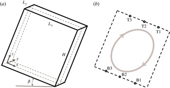
The experiments were carried out in a rectangular cell, as shown in figure 1. Its length
 $L_{x}$
, width
 $L_{y}$
and height
 $H$
are
 $257\ \text{mm}\times 65\ \text{mm}\times 257\ \text{mm}$
, which correspond to the aspect ratios
 ${\it\Gamma}_{x}=L_{x}/H=1$
and
 ${\it\Gamma}_{y}=L_{y}/H=0.25$
. With this geometry, rotational symmetry does not exist and only a single-roll LSC is expected, mainly confined within the plane of
 ${\it\Gamma}_{x}=1$
. The working fluid is water, with
 $\mathit{Pr}\simeq 6.3$
. The experimental apparatus and set-up are similar to those described by Xia et al. (Reference Xia, Sun and Zhou2003) and Zhou et al. (Reference Zhou, Sun and Xia2007), except that the cell size is smaller here. The top and bottom plates are made of copper, and the sidewall is made of Plexiglas. The temperature of the top plate is kept constant at 16.63 °C by a refrigerated circulator (Polyscience Model 9702) with a temperature stability of
 $\pm 0.01\,^{\circ }\text{C}$
. An electric heater pad, connected to the DC power supply, is inserted into the bottom plate to provide the heating power. When the cell-tilt angle varies, the electric power is adjusted to keep the temperature difference between the bottom and top plates
 ${\rm\Delta}T\ (=14.37\pm 0.06\,^{\circ }\text{C})$
approximately constant, corresponding to the Rayleigh number (
 $\mathit{Ra}=4.42\times 10^{9}$
). Six thermistors are embedded into the top and bottom plates to monitor the temperature of the plates, as shown in figure 1(b). The resistances of the thermistors are recorded by a digital multimeter (Keithley Model 2700) with a sampling rate of 4 Hz. The corresponding temperature is then converted from the resistances according to calibration curves. For each run, the left side of the cell is carefully tilted and fixed by a stainless-steel frame to achieve the tilt angle
 ${\it\beta}$
(ranging from 0 to
 ${\rm\pi}/2\ \text{rad}$
).
(a) Schematic diagram of the convection cell and the coordinate frame of the experiments. The length, width and height of the cell are represented by
 $L_{x}$
,
 $L_{y}$
and
 $H$
, respectively, and
 ${\it\beta}$
is the cell-tilting angle relative to the horizontal. The
 $x$
and
 $z$
coordinate axes are along the bottom plate and the sidewall in the LSC plane, and the
 $y$
coordinate axis is perpendicular to the LSC plane. The coordinate frame moves with the angle
 ${\it\beta}$
. (b) The
 $x\text{{-}}z$
cross-sectional plane of the cell at
 $y=0$
(shown as the dashed plane in (a)). Inside the plane, the LSC flow is indicated by the grey ellipse. Six thermistors are embedded in the top and bottom plates at the positions T1 to T3 and B1 to B3.

Besides the temperature measurements, the velocity field in the mid-width plane at
 $y=0$
is measured using PIV. As shown in figure 1(a), the coordinate frame is set in terms of the mid-width plane. The origin is at the bottom left corner, the
 $x$
and
 $z$
axes are along the bottom plate and the sidewall, respectively, and the
 $y$
axis points inwards. The velocity components
 $u$
and
 $w$
are in the
 $x$
and
 $z$
directions, respectively. The application of PIV to the RBC system has been described in previous works (Xia et al.
Reference Xia, Sun and Zhou2003; Sun, Xia & Tong Reference Sun, Xia and Tong2005b
; Wei & Xia Reference Wei and Xia2013). In the present study, a double-cavity neodymium-doped yttrium aluminium garnet (Nd:YAG) laser, with an interval time 0.068 s, provides a light sheet (
 ${\sim}3\ \text{mm}$
thick) to illuminate the convection cell. Polyamide seeding particles (
 ${\sim}20\ {\rm\mu}\text{m}$
,
 ${\it\rho}=1.03\ \text{g}\ \text{cm}^{-3}$
) are used to visualize the flow. The charge-coupled device (CCD) camera has
 $2048\times 2048\ \text{pixels}$
, and the capture rate is 1 Hz. For the measurements, the camera is tilted with the same angle as that of the cell, so that the whole flow field of the LSC plane can be captured. In data analysis, an interrogation window with
 $32\times 32\ \text{pixels}$
is used. As there is a 50 % overlap with adjacent interrogation windows,
 $127\times 127$
vectors can be obtained in each velocity map, which leads to the spatial resolution of 2.02 mm in the
 $x$
and
 $z$
directions. The errors in the velocity vectors and their positions are approximately
 $\pm 1.8\times 10^{-4}\ \text{m}\ \text{s}^{-1}$
and
 $\pm 0.1\ \text{mm}$
, respectively. The first available vectors are typically at a distance of
 ${\sim}3\ \text{mm}$
from the walls. Depending on the tilt angle
 ${\it\beta}$
, a waiting period of between 6 and 24 h was required to obtain a stable flow state, after which two 1 h PIV measurements were recorded with a time interval of 2 h.
To minimize the heat loss, both conductive plates and the sidewall are covered with several Styrofoam insulation layers. The apparatus is placed in a thermostatic chamber, which has a temperature close to that of the bulk flow, to reduce heat exchange between the fluid and the surroundings. The thermostatic chamber is made of Plexiglas sheets and its temperature stability is better than
 $\pm 1\,^{\circ }\text{C}$
. The PIV measurements required the removal of the sidewall insulation layers.
3. Results and discussion
3.1. The velocity field
Using the PIV velocity measurements, we are able to describe the flow field as a function of tilt angle
 ${\it\beta}$
. PIV measurements of RBC in a horizontal rectangular cell with
 ${\it\Gamma}\simeq 1$
have been reported by Xia et al. (Reference Xia, Sun and Zhou2003). In their experiments, the distinct features of the mean flow field were well described in terms of a central low-velocity elliptical core, two high-velocity bands outside of the central core, and two counter-rotating vortices at the cell corners. Among these flow structures, the high-velocity band reflects one of the basic characteristics of the LSC, and is the main focus in the following discussion.
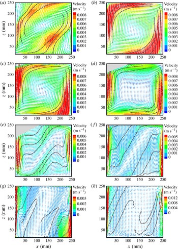
Coarse-grained vector map of the time-averaged velocity field for an angle
 ${\it\beta}$
of (a) 0, (b) 0.15, (c) 0.23, (d) 0.64, (e) 0.92, ( f) 1.05, (g) 1.17 and (h) 1.41 rad. At each
 ${\it\beta}$
, the velocity magnitude is scaled by the different colour bar. The trajectories produced by the Tecplot software are plotted to highlight the flow pattern. At (d)
 ${\it\beta}=0.64\ \text{rad}$
and (e)
 ${\it\beta}=0.92\ \text{rad}$
, some velocity distortions in the upper left corner manifest due to the weak laser light, and are shaded.

Figure 2 shows the time-averaged velocity maps at eight different tilt angles. Note that here the velocity vectors have been further averaged by using a
 $3\times 3$
window, so that they can be more clearly exhibited. The velocity magnitude
 $V$
is defined as
 $V=\sqrt{U^{2}+W^{2}}$
, where
 $U$
and
 $W$
are the time-averaged velocity components along the
 $x$
and
 $z$
axes, respectively. In the level case (figure 2
a), a clear clockwise LSC spans the whole cell, with two counter-rotating eddies at the upper left and lower right corners. These flow features are similar to those described by Xia et al. (Reference Xia, Sun and Zhou2003). As
 ${\it\beta}$
increases from 0 to 0.64 rad (figure 2
a–d), the pattern of the LSC gradually changes from oblique ellipse-like to square-like. Meanwhile, the counter-rotating eddies seem to disappear. In previous studies it was reported that the LSC pattern shifted from an elliptical shape at low Rayleigh numbers to a squarish shape at high Rayleigh numbers in a level cell (Niemela & Sreenivasan Reference Niemela and Sreenivasan2003; Xia et al.
Reference Xia, Sun and Zhou2003). The present observations may suggest that the increasing value of
 ${\it\beta}$
plays the same role as the increasing value of
 $\mathit{Ra}$
in modifying the LSC pattern. When
 ${\it\beta}$
is increased further the flow pattern becomes relatively complicated. At
 ${\it\beta}=0.92\ \text{rad}$
(figure 2
e), the flow along the sidewall first strikes the lower right (or upper left) corner, then bounces towards the bulk region, but finally turns back to the plates. That is, the flow moves in a tortuous way. At
 ${\it\beta}=1.05\ \text{rad}$
(figure 2
f), the flow pattern is similar to that at
 ${\it\beta}=0.92\ \text{rad}$
, but the bouncing height seems to be greater. In both cases, a single LSC can still be discernible. At
 ${\it\beta}=1.17\ \text{rad}$
(figure 2
g), the high-velocity band is still adjoining the sidewall, and two large backflows occur in the right and left halves of the cell. For
 ${\it\beta}\geqslant 1.41\ \text{rad}$
, the bulk region is full of small chaotic flow structures, which cannot be well distinguished because of the extremely slow flow speed. Generally, figure 2 shows that the high-velocity zone approaches the sidewall and departs from the conductive plates as the tilt angle
 ${\it\beta}$
increases.
In order to quantify the global flow pattern, it is assumed that there is still a single large-scale flow roll in the convection cell. The origin of the roll is defined to be the cell centre; then the position (
 $x,z$
) is transformed into (
 $r,{\it\theta}$
), where
 $r$
is the polar radius and
 ${\it\theta}$
is the polar angle. Usually, the velocity profiles along
 $x=L_{x}/2$
and
 $z=H/2$
are analysed in order to characterize the LSC (Qiu & Tong Reference Qiu and Tong2001; Xia et al.
Reference Xia, Sun and Zhou2003). Here, an alternative strategy is applied using the azimuthal average velocity,
 $V_{a}$
, so that the global flow field can be involved. However, as shown in figure 2, the LSC pattern is affected by the square shape of the cell. Thus, when the azimuthal average velocity,
 $V_{a}$
, is examined, it makes sense to analyse the velocity of the same
 $r/r_{b}$
, where
 $r_{b}$
is the distance between the boundary and the cell centre and with the same
 ${\it\theta}$
as
 $r$
. Therefore, the azimuthal average velocity
 $V_{a}$
has the form
 $$\begin{eqnarray}V_{a}(r/r_{b})=\frac{1}{N_{r/r_{b}}}\mathop{\sum }_{r-{\it\delta}r}^{r+{\it\delta}r}\mathop{\sum }_{{\it\theta}=0}^{2{\rm\pi}}V(r/r_{b},{\it\theta}),\end{eqnarray}$$
where
 ${\it\delta}r=r_{b}/100$
and
 $N_{r/r_{b}}$
is the number of velocity vectors along the normalized radius
 $r/r_{b}$
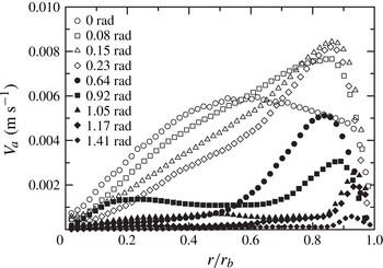
. Figure 3 shows the circulating velocity
 $V_{a}$
as a function of the normalized radius
 $r/r_{b}$
for different tilt angles. It indicates that the
 $V_{a}$
profile varies with the tilt angle
 ${\it\beta}$
. Generally, a velocity peak appears in each
 $V_{a}$
profile, which corresponds to the high-velocity band of the LSC. Therefore, the LSC can be described using the amplitude
 $V_{ap}$
, position
 $(r/r_{b})_{p}$
and width
 $hw/r_{b}$
of the velocity peak.
The azimuthal average velocity
 $V_{a}$
as a function of the normalized radius
 $r/r_{b}$
at
 ${\it\beta}=0$
, 0.08, 0.15, 0.23, 0.64, 0.92, 1.05, 1.17 and 1.41 rad (as indicated).

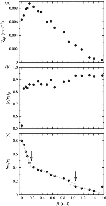
(a) The amplitude (
 $V_{ap}$
), (b) position (
 $(r/r_{b})_{p}$
) and (c) width (
 $hw/r_{b}$
) of the high-velocity band as functions of the tilt angle (
 ${\it\beta}$
). In (c), the three grey lines are least-squares linear fits for
 $0\leqslant {\it\beta}\leqslant 0.15\ \text{rad}$
,
 $0.15<{\it\beta}<1.05\ \text{rad}$
and
 $1.05\leqslant {\it\beta}<{\rm\pi}/2\ \text{rad}$
, with slopes
 $-2.2$
,
 $-0.3$
and
 $-0.17\ \text{rad}^{-1}$
, respectively.

The results obtained for the amplitude
 $V_{ap}$
are shown in figure 4(a). First,
 $V_{ap}$
increases with increasing
 ${\it\beta}$
, before reaching a maximum at
 ${\it\beta}\simeq 0.15\ \text{rad}$
. After this,
 $V_{ap}$
gradually decreases as
 ${\it\beta}$
increases further. The position of the high-velocity band has a different
 ${\it\beta}$
dependence. As shown in figure 4(b), the high-velocity band concentrates at
 $(r/r_{b})_{p}\simeq 0.5$
(about a quarter width from the boundary) in the level case (
 ${\it\beta}=0\ \text{rad}$
). When the cell is slightly tilted (
 ${\it\beta}=0.04\ \text{rad}$
), the high-velocity band moves abruptly towards the cell boundary (
 $(r/r_{b})_{p}\simeq 0.83$
). As
 ${\it\beta}$
increases further to
 ${\rm\pi}/2\ \text{rad}$
, even though the data are somewhat scattered, the high-velocity band can be seen to progressively approach the boundary to
 $(r/r_{b})_{p}\simeq 0.93$
. The position of the high-velocity band shows that the LSC has different flow patterns between the level and tilted cases. In the level case, the convection cell is axisymmetric with respect to the cell’s vertical centreline, and so is the buoyancy force produced from the conductive plates. It should not matter whether the LSC flow is clockwise or anticlockwise, accompanied with the large eddies in the corners (figure 2
a). In the tilted case, the buoyancy force of the system is no longer axisymmetric with respect to the cell’s vertical centreline, the LSC is forced into a certain flow direction (Ahlers et al.
Reference Ahlers, Brown and Nikolaenko2006) and the eddies inside the corners are strongly suppressed. The LSC pattern is, therefore, very sensitive to the symmetry of the system. The width of the high-velocity band,
 $hw/r_{b}$
, is defined as the width at half the velocity amplitude,
 $V_{ap}$
, in the velocity profile (figure 3). Figure 4(c) shows the values obtained for the width
 $hw/r_{b}$
. These indicate that the width
 $hw/r_{b}$
decreases with increasing
 ${\it\beta}$
. It seems that there are two transitions at
 ${\it\beta}=0.15\ \text{rad}$
and
 ${\it\beta}=1.05\ \text{rad}$
. The reduction slopes are 2.2, 0.3 and
 $0.17\ \text{rad}^{-1}$
in the ranges
 $0\leqslant {\it\beta}\leqslant 0.15\ \text{rad}$
,
 $0.15<{\it\beta}<1.05\ \text{rad}$
and
 $1.05\leqslant {\it\beta}<{\rm\pi}/2\ \text{rad}$
, respectively. Note that the width,
 $hw/r_{b}$
, at
 ${\it\beta}={\rm\pi}/2\ \text{rad}$
is not included in the analysis as it is beyond the low-velocity measurement limit. Recent studies have shown that the aspect ratio
 ${\it\Gamma}_{y}$
also has a strong effect on the flow dynamics and heat transport (Huang et al.
Reference Huang, Kaczorowski, Ni and Xia2013; Wagner & Shishkina Reference Wagner and Shishkina2013). Therefore, the dependence of the LSC on the tilt angle
 ${\it\beta}$
might be different for different
 ${\it\Gamma}_{y}$
.
3.2. Temperature and velocity oscillations
Compared to the cylindrical cell (Cioni et al. Reference Cioni, Ciliberto and Sommeria1997; Chillà et al. Reference Chillà, Rastello, Chaumat and Castaing2004; Sun et al. Reference Sun, Xi and Xia2005a ; Ahlers et al. Reference Ahlers, Brown and Nikolaenko2006), the rectangular cell simplifies the flow dynamics by lowering the degrees of freedom of the LSC. Twisting and sloshing of the LSC are expected to be suppressed in this quasi-two-dimensional case, possibly influencing the temperature and velocity oscillation. Therefore, it is worth examining the dependence of the oscillation intensity and period on the tilt angle in both temperature and velocity fields. Generally, the coherent oscillation is examined by analysing the autocorrelation function,
 $$\begin{eqnarray}C_{X}({\it\tau})=\frac{\langle {\it\delta}X_{i}(t){\it\delta}X_{i}(t+{\it\tau})\rangle }{\langle {\it\delta}X_{i}(t)^{2}\rangle },\end{eqnarray}$$
where
 $X$
can be temperature or velocity,
 ${\it\delta}X$
is the fluctuation in
 $X$
, the subscript
 $i$
denotes the sample position and the angle brackets denote the time average. The intensity (
 $I$
) and period (
 ${\it\tau}_{o}$
) of oscillation are defined as the amplitude and time period of the second-order peak in the autocorrelation function, respectively.
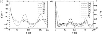
Figure 5(a) shows an example of the temperature autocorrelation functions measured by the six thermistors in the plates at
 ${\it\beta}=0.38\ \text{rad}$
. An obvious oscillation (
 ${\it\tau}_{o}=80.7\pm 1.7\ \text{s}$
) can be identified in all autocorrelation functions, even though the oscillation intensity is different at different positions. In the bottom plate, the oscillation intensity is strongest at position B1, as shown in figure 1(b), where the cold descending flow arrives. The intensity gets weaker and weaker from right to left (from B1 to B3). Similar observations are found at the top plate, where the intensity is weakened from left to right (from T3 to T1). This result is somewhat similar to that in the cylindrical cell (Xi et al.
Reference Xi, Zhou, Zhou, Chan and Xia2009), where the oscillations are also found at the positions of plume impingement and are absent at the positions of plume emission. At other tilt angles, the strongest oscillations are always found at positions B1 and T3, too.
(a) Autocorrelation functions of the temperature signals at the six thermistor positions in the plates for
 ${\it\beta}=0.38\ \text{rad}$
. (b) Autocorrelation functions of the velocity component,
 $w$
, at the eight positions for
 ${\it\beta}=0.38\ \text{rad}$
. These positions are described in the text.

Eight positions are selected to examine the oscillation in the velocity signals. Three of them are 15 mm above B1, B2 and B3 and are denoted by Bv1, Bv2 and Bv3, respectively. The other three positions are 12 mm below T1, T2 and T3 and are denoted by Tv1, Tv2 and Tv3, respectively. In addition, we select a position at the mid-height of the cell and approximately 25 mm from the sidewall, denoted by S1. The last position is in the centre, denoted by C1. At each position it is found that the velocity components
 $u$
and
 $w$
have more or less the same autocorrelation functions. Therefore, only the velocity
 $w$
is used for the oscillation analysis. The autocorrelation functions of
 $w$
at these eight positions for
 ${\it\beta}=0.38\ \text{rad}$
are shown in figure 5(b). They indicate that an obvious oscillation with a period of
 ${\sim}80\ \text{s}$
appears, which is consistent with the observations in the temperature signals (figure 5
a). At positions Bv1 and Tv3, the oscillation is found to be strongest, also consistent with the temperature observation. The oscillation is found to be very obvious near the sidewall (at position S1), where the oscillation intensity is nearly as strong as those at positions Bv1 and Tv3. On the other hand, the oscillation is weakest in the cell centre (at position C1). Therefore, the oscillation distributions near the sidewall and in the centre are consistent with the previous observations in the level case (Zhou et al.
Reference Zhou, Sun and Xia2007).
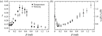
As shown in figure 5, the intensity of oscillation is the strongest, and is almost the same at the positions B1 (Bv1) and T3 (Tv3) in temperature (velocity) signals. We can use the average intensity at these two positions to represent the temperature (velocity) oscillation of the whole system. Figure 6(a) shows the oscillation intensity (
 $I$
) as a function of the tilt angle
 ${\it\beta}$
. Within the experimental errors, the oscillation intensity
 $I$
follows similar trends for the temperature and velocity signals. It first increases with increasing
 ${\it\beta}$
, until it reaches its maximum at around
 ${\it\beta}\simeq 0.48\ \text{rad}$
, before decreasing as
 ${\it\beta}$
is increased further. For
 ${\it\beta}>1.05\ \text{rad}$
, the oscillation is not detectable in the temperature autocorrelation function at all thermistor positions. For
 ${\it\beta}>1.32\ \text{rad}$
, the oscillation cannot be detected in the velocity signals either. Figure 6(b) shows the oscillation period
 ${\it\tau}_{o}$
as a function of the tilt angle
 ${\it\beta}$
. The temperature and velocity oscillation periods agree well with each other. With increasing
 ${\it\beta}$
,
 ${\it\tau}_{o}$
first decreases, it has a remarkable transition at an angle of approximately
 ${\it\beta}=0.15\ \text{rad}$
, then it increases gradually as
 ${\it\beta}$
increases from 0.15 to 1.32 rad.
(a) Oscillation intensity (
 $I$
) and (b) oscillation period (
 ${\it\tau}_{o}$
) as functions of the tilt angle
 ${\it\beta}$
from temperature and velocity signals.

3.3. The Reynolds numbers
In this section, the Reynolds number, which is defined as
 $\mathit{Re}=LV/{\it\nu}$
, is discussed using several characteristic speeds for
 $V$
. In RBC, the oscillation period is comparable to the complete turnover time of the single LSC, for aspect ratios close to one (Ahlers et al.
Reference Ahlers, Brown and Nikolaenko2006; Zhou et al.
Reference Zhou, Sun and Xia2007; Weiss & Ahlers Reference Weiss and Ahlers2013). Thus, the Reynolds number
 $\mathit{Re}_{o}$
, based on the oscillation period (
 ${\it\tau}_{o}$
), can be defined as
 $$\begin{eqnarray}\mathit{Re}_{o}=\frac{L}{{\it\nu}}\frac{4L}{{\it\tau}_{o}},\end{eqnarray}$$
where
 ${\it\tau}_{o}$
is the average oscillation period from the temperature and velocity signals at the same tilt angle
 ${\it\beta}$
. In addition, the maximum velocity of the whole velocity field,
 $V_{m}$
, is selected, which corresponds to the Reynolds number
 $\mathit{Re}_{m}$
. As mentioned in § 3.1,
 $V_{ap}$
is the velocity amplitude of the LSC, with the corresponding Reynolds number being denoted by
 $\mathit{Re}_{ap}$
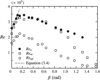
. The results are shown in figure 7. It is interesting that
 $\mathit{Re}_{o}$
and
 $\mathit{Re}_{m}$
are more or less the same over the
 ${\it\beta}$
range between 0 and 1.05 rad, and their deviation appears and gets larger as
 ${\it\beta}$
increases. This is probably caused by complicated flow patterns in the bulk region, such as the backflows shown in figure 2(g). Compared to
 $\mathit{Re}_{o}$
,
 $\mathit{Re}_{ap}$
has a smaller magnitude, which should be due to the different definitions of the characteristic speed. The various Reynolds numbers
 $\mathit{Re}_{o}$
,
 $\mathit{Re}_{m}$
and
 $\mathit{Re}_{ap}$
have a common trend. With increasing
 ${\it\beta}$
, the
 $\mathit{Re}$
number first increases until it reaches its maximum at approximately
 ${\it\beta}=0.15\ \text{rad}$
, after which it gradually decreases.
The Reynolds numbers,
 $\mathit{Re}_{o}$
,
 $\mathit{Re}_{m}$
and
 $\mathit{Re}_{ap}$
, as functions of the tilt angle
 ${\it\beta}$
. Equation (3.4) is plotted as a grey dashed line.

For small values of
 ${\it\beta}$
, Chillà et al. (Reference Chillà, Rastello, Chaumat and Castaing2004) and Ahlers et al. (Reference Ahlers, Brown and Nikolaenko2006) also found that cell tilting leads to an enhancement of the Reynolds number of the LSC. Chillà et al. (Reference Chillà, Rastello, Chaumat and Castaing2004) modelled this by considering the equilibrium of the buoyancy and shear forces for the top and bottom boundary layer. Ahlers et al. (Reference Ahlers, Brown and Nikolaenko2006) deduced that the Reynolds number is of the form
 $$\begin{eqnarray}\mathit{Re}=\mathit{Re}(0)\left(1+\frac{\mathit{Ra}}{8\,\mathit{Re}(0)\mathit{Pr}\,\mathit{Nu}^{2}}{\it\beta}\right),\end{eqnarray}$$
where
 $\mathit{Re}(0)$
is the Reynolds number at
 ${\it\beta}=0$
, and the Reynolds number is based on the oscillation period. By substituting the present experimental parameters, we can obtain
 $\mathit{Re}=\mathit{Re}(0)(1+3.56{\it\beta})$
. This model is shown as the grey dashed line in figure 7; it agrees with the data for small angles (
 ${\it\beta}<0.15\ \text{rad}$
). As the model predicts that the Reynolds number increases with increasing angle
 ${\it\beta}$
, however, it cannot explain the observation of a decreasing trend at larger values of
 ${\it\beta}$
.
3.4. Heat transport
Lastly, the heat transport of thermal convection is discussed. The calculation of
 $\mathit{Nu}$
needs the values of the heat flux
 $F_{T}$
and the temperature difference
 ${\rm\Delta}T$
. Considering the variances of these quantities, the main measurement error comes from the temperature inhomogeneity of the plates, which is less than 2 % for all tilt angles. When the cell is level, the value of
 $\mathit{Nu}$
is calculated to be 97.8 at
 $\mathit{Ra}=4.42\times 10^{9}$
. In a recent experiment with a rectangular cell with
 ${\it\Gamma}_{x}=1$
and
 ${\it\Gamma}_{y}=0.3$
,
 $\mathit{Nu}=99.3$
has been obtained at
 $\mathit{Ra}=4.6\times 10^{9}$
and
 $\mathit{Pr}=7$
(Zhou et al.
Reference Zhou, Liu, Li and Zhong2012). This is close to the present measurement. As the thermal boundary condition at each
 ${\it\beta}$
is almost the same, e.g. the temperatures of the plates are kept constant, additional heat transport corrections, such as heat leakage (Xia, Lam & Zhou Reference Xia, Lam and Zhou2002), sidewall coupling (Ahlers & Xu Reference Ahlers and Xu2001) and finite plate conductivity (Nikolaenko et al.
Reference Nikolaenko, Brown, Funfschilling and Ahlers2005), have not been applied to avoid new artificial errors.
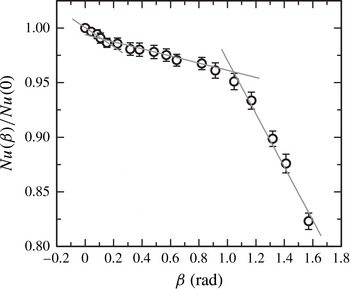
The value of
 $\mathit{Nu}$
as a function of the tilt angle
 ${\it\beta}$
is shown in figure 8. This indicates that cell tilting causes a pronounced reduction of
 $\mathit{Nu}$
. In the range of
 $0\leqslant {\it\beta}\leqslant 0.15\ \text{rad}$
, the reduction of
 $\mathit{Nu}$
is approximately 1.4 % and the decay slope is
 $8.57\times 10^{-2}\ \text{rad}^{-1}$
. This result is significantly different from those reported by Chillà et al. (Reference Chillà, Rastello, Chaumat and Castaing2004) and Weiss & Ahlers (Reference Weiss and Ahlers2013) in cylindrical cells with
 ${\it\Gamma}=0.5$
. Chillà et al. (Reference Chillà, Rastello, Chaumat and Castaing2004) found that
 $\mathit{Nu}$
decreased by 5 % for tilt angles as small as
 ${\it\beta}=0.026\ \text{rad}$
and the decay slope was
 $2\ \text{rad}^{-1}$
, while Weiss & Ahlers (Reference Weiss and Ahlers2013) found that a small value of
 ${\it\beta}$
could slightly enhance the heat transport. Comparatively, the dependence of
 $\mathit{Nu}$
is more or less similar to that in a cylindrical cell of
 ${\it\Gamma}=1$
, where the decay slope is smaller (
 $(3.1\pm 0.1)\times 10^{-2}\ \text{rad}^{-1}$
) (Ahlers et al.
Reference Ahlers, Brown and Nikolaenko2006). In the range of
 $0.15\leqslant {\it\beta}\leqslant 1.05\ \text{rad}$
, the decay slope of
 $\mathit{Nu}$
becomes smaller, and it is fitted as
 $3.27\times 10^{-2}\ \text{rad}^{-1}$
. Coincidentally, this decay slope is close to that in the cylindrical cell of
 ${\it\Gamma}=1$
over a smaller
 ${\it\beta}$
range (Ahlers et al.
Reference Ahlers, Brown and Nikolaenko2006). When
 ${\it\beta}$
further increases (
 $1.05\leqslant {\it\beta}\leqslant {\rm\pi}/2\ \text{rad}$
),
 $\mathit{Nu}$
decays quickly with the slope of
 $0.24\ \text{rad}^{-1}$
, which is approximately eight times larger than that for small
 ${\it\beta}\ ({\leqslant}1.05\ \text{rad})$
. Compared to the level case,
 $\mathit{Nu}$
is weakened only by approximately 5 % at
 ${\it\beta}=1.05\ \text{rad}$
, but the reduction reaches approximately 18 % at
 ${\it\beta}={\rm\pi}/2\ \text{rad}$
.
The normalized Nusselt number
 $\mathit{Nu}({\it\beta})/\mathit{Nu}(0)$
as a function of the tilt angle
 ${\it\beta}$
. The three grey lines are least-squares linear functions for
 $0\leqslant {\it\beta}\leqslant 0.15\ \text{rad}$
,
 $0.15\leqslant {\it\beta}\leqslant 1.05\ \text{rad}$
and
 $1.05\leqslant {\it\beta}\leqslant {\rm\pi}/2\ \text{rad}$
, with slopes
 $-8.57\times 10^{-2}$
,
 $-3.27\times 10^{-2}$
and
 $-0.24\ \text{rad}^{-1}$
, respectively.

Combined with the variance of flow dynamics at different values of
 ${\it\beta}$
, the transition at
 ${\it\beta}=0.15\ \text{rad}$
can be observed in the dependences of both
 $\mathit{Re}$
and
 $\mathit{Nu}$
on
 ${\it\beta}$
. However, the heat transport of thermal convection is still reduced, even though the LSC speed is highest, which suggests that the evolution of thermal structures must be considered in understanding the heat transport. The transition at
 ${\it\beta}=1.05\ \text{rad}$
cannot be discerned in the dependence of
 $\mathit{Re}$
on
 ${\it\beta}$
, but seems to be obvious in the dependence of
 $\mathit{Nu}$
on
 ${\it\beta}$
. As shown in figure 2, there are totally different flow patterns when the cell is at
 ${\it\beta}<1.05\ \text{rad}$
and
 ${\it\beta}\geqslant 1.05\ \text{rad}$
, which may be responsible for the variance of
 $\mathit{Nu}$
. Further work, such as an instantaneous
 $\mathit{Nu}$
measurement, is needed in order to understand the dependence of
 $\mathit{Nu}$
on
 ${\it\beta}$
.
4. Summary
In this paper, we carried out an experimental investigation of the flow dynamics and heat transport in turbulent RBC within a rectangular cell (
 ${\it\Gamma}_{x}=1$
and
 ${\it\Gamma}_{y}=0.25$
), at almost constant
 $\mathit{Pr}\ (\mathit{Pr}\simeq 6.3)$
and
 $\mathit{Ra}\ (\mathit{Ra}\simeq 4.42\times 10^{9})$
, over a wide range of tilt angles (
 $0\leqslant {\it\beta}\leqslant {\rm\pi}/2\ \text{rad}$
).
With the velocity field measured by PIV, the influence of cell tilting on the LSC pattern has been examined. It indicates that the LSC pattern changes gradually from oblique ellipse-like to square-like as
 ${\it\beta}$
increases from 0 to 0.64 rad. When
 ${\it\beta}$
increases further, the flow in the bulk region becomes complicated, e.g. two large backflows occur at
 ${\it\beta}=1.17\ \text{rad}$
. The LSC pattern is sensitive to the symmetry of the system. In the level case, the LSC is at about a quarter width (
 $(r/r_{b})_{p}\simeq 0.5$
) of the cell. It moves abruptly towards the boundary (
 $(r/r_{b})_{p}\simeq 0.83$
) as the cell is slightly tilted (
 ${\it\beta}=0.04\ \text{rad}$
). With increasing
 ${\it\beta}$
, the LSC velocity reaches a maximum at
 ${\it\beta}=0.15\ \text{rad}$
. While the LSC width progressively decreases with
 ${\it\beta}$
, two transitions at
 ${\it\beta}=0.15\ \text{rad}$
and
 ${\it\beta}=1.05\ \text{rad}$
occur, depending on different reduction slopes. Oscillations have been found in both temperature and velocity signals for almost all
 ${\it\beta}$
and they are strongest at around
 ${\it\beta}\simeq 0.48\ \text{rad}$
.
By using three velocities to characterize the LSC, including the maximum velocity
 $V_{m}$
, the velocity amplitude of the LSC
 $V_{ap}$
, and the one induced from oscillation period
 ${\it\tau}_{o}$
, the dependence of
 $\mathit{Re}$
on
 ${\it\beta}$
has been found to follow similar trends. With increasing
 ${\it\beta}$
,
 $\mathit{Re}$
first increases until it reaches its maximum at the transition angle
 ${\it\beta}=0.15\ \text{rad}$
, after which it gradually decreases.
Cell tilting causes a pronounced reduction in
 $\mathit{Nu}$
. From 0 to 0.15, 1.05 and
 ${\rm\pi}/2\ \text{rad}$
, the reduction of
 $\mathit{Nu}$
is 1.4 %, 5 % and 18 %, respectively. Over the ranges
 $0\leqslant {\it\beta}\leqslant 0.15\ \text{rad}$
,
 $0.15\leqslant {\it\beta}\leqslant 1.05\ \text{rad}$
and
 $1.05\leqslant {\it\beta}\leqslant {\rm\pi}/2\ \text{rad}$
, the decay slope is
 $8.57\times 10^{-2}$
,
 $3.27\times 10^{-2}$
and
 $0.24\ \text{rad}^{-1}$
, respectively. The transition angles
 ${\it\beta}=0.15\ \text{rad}$
and
 ${\it\beta}=1.05\ \text{rad}$
can also be observed in the description of the LSC character; however, the dependence of
 $\mathit{Nu}$
on
 ${\it\beta}$
is different from that of
 $\mathit{Re}$
, which may suggest that detailed measurements of the temperature field are needed in future studies.
Acknowledgements
We gratefully acknowledge W. Wang for valuable discussions. This work was supported by China NSF grants (41176027, 41476167 and 41406035), the Strategic Priority Research Program of the Chinese Academy of Sciences (XDA11030302) and LTO grant (LTOZZ1304).