







1. Introduction
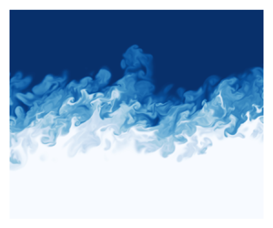
Many turbulent mixing problems can be characterized by a sharp interface separating two regions of flow, e.g. the flame surface in both premixed and non-premixed flames, which separates fresh from burnt fuel (premixed) and fuel from oxidizer (non-premixed), or the turbulent/non-turbulent (T/NT) interface which separates turbulent, rotational flow from the irrotational, quiescent background in turbulent shear flows. An important similarity between these seemingly disparate problems is that the interface can be described by an isosurface of a scalar field. For example, the flame surface in premixed combustion can be described by an isosurface of a progress variable (typically temperature or species mass fraction) coinciding with the peak reaction rate (Candel & Poinsot Reference Candel and Poinsot1990), while the flame surface in non-premixed reactions is typically described by an isosurface of the mixture fraction corresponding to the stoichiometric mixture of fuel and oxidizer (Peters Reference Peters1988). Moreover, the T/NT interface can be typically demarcated by a ‘small’ value of the vorticity magnitude (da Silva et al. Reference da Silva, Hunt, Eames and Westerweel2014).
The kinematics of these interfaces is directly related to important quantities for engineering design and optimization. For instance, knowledge of the flame surface area allows the net fuel consumption to be computed (Marble & Broadwell Reference Marble and Broadwell1977). Similarly, the entrainment rate of ambient fluid into the turbulent core of a jet or wake is proportional to the surface area of the T/NT interface (Wolf et al. Reference Wolf, Lüthi, Holzner, Krug, Kinzelbach and Tsinober2012). Clearly, a fundamental understanding of isosurfaces embedded in turbulent flows is needed to properly characterize such systems with dynamic sources and sinks of isosurface area. With proper characterization, it may be possible to improve predictive models of these interfacial systems.
Unfortunately, experimental measurement of isosurfaces in turbulent flows is both difficult and expensive. Advances in experimental technology have allowed for impressive measurements of both the T/NT interface and flame surface, such as recent experiments by Balamurugan et al. (Reference Balamurugan, Rodda, Philip and Mandal2020) and Skiba et al. (Reference Skiba, Wabel, Carter, Hammack, Temme and Driscoll2018). However, even state of the art experiments typically measure only two-dimensional statistics, which cannot recover the fully three-dimensional behaviour of isosurfaces embedded in a turbulent flow. Direct numerical simulation, on the other hand, coupled with recent advances in computing power and numerical algorithms, allows for in-depth investigation into high-resolution, three-dimensional velocity and scalar fields. Despite being restricted to relatively simple geometries, direct numerical simulation (DNS) is a valuable tool for studying fundamental properties of turbulence such as interfacial dynamics.
Much of the literature surrounding the T/NT interface is focused on characterizing the topology and internal structure of the interface, with significant advances occurring in the last two decades. A comprehensive review is given by da Silva et al. (Reference da Silva, Hunt, Eames and Westerweel2014), where many important characteristics of the interface are discussed, such as the scaling of the viscous and turbulent sublayers, the relative importance of engulfment and nibbling on entrainment, and the effect of large-scale motions on the interface. Since then, others have examined how the interface thickness scales with Reynolds number (Silva, Zecchetto & da Silva Reference Silva, Zecchetto and da Silva2018), investigated the role of coherent structures on interface properties (Neamtu-Halic et al. Reference Neamtu-Halic, Krug, Mollicone, Reeuwijk, Van Haller and Holzner2020) and expanded the T/NT interface analysis to stratified (Watanabe et al. Reference Watanabe, Riley, de Bruyn Kops, Diamessis and Zhou2016) and compressible (Jahanbakhshi & Madnia Reference Jahanbakhshi and Madnia2018; Zhang, Watanabe & Nagata Reference Zhang, Watanabe and Nagata2018) flows.
Similarly, a number of studies have examined the structure (e.g. Sankaran et al. Reference Sankaran, Hawkes, Yoo and Chen2015; Wang et al. Reference Wang, Hawkes, Chen, Zhou, Li and Aldén2017) and topology (e.g. Wacks et al. Reference Wacks, Chakraborty, Klein, Arias and Im2016; Dopazo et al. Reference Dopazo, Martin, Cifuentes and Hierro2018) of the flame surface in premixed combustion. Significant focus has also been placed on the flame surface area per unit volume,  $\varSigma$, which, in combination with the premixed flame speed, is directly proportional to the rate of fuel consumption (Poinsot & Veynante Reference Poinsot and Veynante2005). Studies have examined the effects of turbulence intensity (Kim & Pitsch Reference Kim and Pitsch2007), differential diffusion (Chakraborty, Klein & Swaminathan Reference Chakraborty, Klein and Swaminathan2009) and detailed chemistry (Klein et al. Reference Klein, Herbert, Kosaka, Böhm, Dreizler, Chakraborty, Papapostolou, Im and Hasslberger2020) on the flame surface area density, among others.
While obviously beneficial for a global understanding of both the T/NT interface and flame surface, the studies listed above tend to focus on instantaneous snapshots of temporally or spatially developing flows (in the case of T/NT interface), or on integrated surface quantities in statistically stationary flows (flame surface). There has only been a single study, to the authors’ knowledge, that has presented both the spatial and temporal variation of the flame surface density (Kulkarni et al. Reference Kulkarni, Buttay, Kasbaoui, Attili and Bisetti2021). In this study of spherically expanding premixed flames, the flame surface area density is plotted as a function of the radial direction and at several instances in time (see Kulkarni et al. Reference Kulkarni, Buttay, Kasbaoui, Attili and Bisetti2021, figure 9), demonstrating that the flame surface area is distributed over a finite region of physical space, and that this distribution is expected to vary in time and/or space, depending on the flow conditions.
From the above discussion, it can be seen that an investigation of the spatial and temporal development of an isosurface embedded in a turbulent flow field is an important step towards understanding the behaviour of a broad class of turbulent mixing problems. In this paper, results are presented from a DNS of a passive scalar field evolving in a temporally developing mixing layer. Though phenomenological differences exist between the isosurface of a passive scalar field and the T/NT interface or the premixed flame surface discussed above, a passive scalar such as dye is commonly used to demarcate the T/NT interface (Westerweel et al. Reference Westerweel, Fukushima, Pedersen and Hunt2005), and there is evidence to suggest that premixed flames subjected to intense turbulence behave similarly to passive scalars (Savard & Blanquart Reference Savard and Blanquart2015). A computationally efficient, grid-based approach (Yurtoglu, Carton & Storti Reference Yurtoglu, Carton and Storti2018) for calculating surface integrals is utilized that allows for the isosurface properties, namely the isosurface area and isosurface area density, to be tracked throughout the temporal development of the mixing layer. The paper is organized as follows. Section 2 describes the computational methodology of the DNS, § 3 presents the basic mathematical background of isosurface area; § 4 provides typical velocity and scalar statistics to validate the simulation accuracy; § 5 details the primary results from the study, including the self-similar analysis of the isosurface area and isosurface area density; § 6 summarizes the conclusions and discusses potential future research.
2. Computational set-up
For the DNS presented below, a custom version of the code base MIRANDA is used. The software was developed at Lawrence Livermore National Laboratory (LLNL) and can perform both DNS and large-eddy simulation (LES) in high energy density applications. MIRANDA has been validated extensively and used for several other novel research cases such as the Rayleigh–Taylor, Kelvin–Helmholtz and Richtmeyer–Meshkov instabilities (Cook, Cabot & Miller Reference Cook, Cabot and Miller2004; Olson et al. Reference Olson, Larsson, Lele and Cook2011; Tritschler et al. Reference Tritschler, Olson, Lele, Hickel, Hu and Adams2014). The particular version utilized for this study is part of an ongoing effort to port MIRANDA to heterogeneous architectures, which contain both traditional central processing units as well as novel graphics processing units. This section will briefly outline the governing equations and numerical methods of MIRANDA, but interested readers are encouraged to consult Cook (Reference Cook2007, Reference Cook2009) for more details regarding MIRANDA, and Rieben et al. (Reference Rieben2020) for more information regarding the graphics processing unit porting effort.
2.1. Governing equations
MIRANDA solves the three-dimensional, compressible Navier–Stokes equations
 \begin{gather} \frac{\partial \rho}{\partial t} + \frac{\partial \rho U_i}{\partial x_i} = 0, \end{gather}
 \begin{gather}\frac{\partial \rho U_i}{\partial t} + \frac{\partial \rho U_iU_j}{\partial x_j} ={-}\frac{\partial P}{\partial x_i} + \frac{\partial {\boldsymbol{\mathsf{\tau}}} _{ij}}{\partial x_j}, \end{gather}
 \begin{gather}\frac{\partial E}{\partial t} + \frac{\partial (E+P)U_i}{\partial x_i} = \frac{\partial {\boldsymbol{\mathsf{\tau}}} _{ij}U_j}{\partial x_i} + \frac{\partial q_i}{\partial x_i}, \end{gather}
where  $\rho$ is the fluid density,
 $U_i$ is the velocity,
 $P$ is pressure,
 ${\boldsymbol{\mathsf{\tau}}} _{ij}$ is the ijth component of the viscous stress tensor,
 $E$ is the total energy (internal plus kinetic) and
 $q_i$ is the ith component of the conductive heat flux vector. For a Newtonian fluid, invoking Stokes’ hypothesis, the viscous stress tensor is given by
 \begin{equation} {\boldsymbol{\mathsf{\tau}}} _{ij} = 2\mu \left({\mathsf{S}}_{ij} - \frac{1}{3}\frac{\partial U_k}{\partial x_k}\delta_{ij}\right), \end{equation}
where  $\delta _{ij}$ is the Kronecker delta,
 $\mu$ is the dynamic viscosity and
 ${\mathsf{S}}_{ij}$ is the strain-rate tensor (Kundu & Cohen Reference Kundu and Cohen2002)
 \begin{equation} {\mathsf{S}}_{ij} = \frac{1}{2}\left(\frac{\partial U_i}{\partial x_j} + \frac{\partial U_j}{\partial x_i} \right). \end{equation}
The total energy  $E$ is given by
 \begin{equation} E = \rho(e + U_iU_i/2), \end{equation}
where  $e$ is the internal energy per unit mass, and the heat flux
 $q_i$ is given by Fourier's Law
 \begin{equation} q_i = \kappa \frac{\partial T}{\partial x_i}, \end{equation}
with  $\kappa$ as the thermal conductivity. To close the above equations, the gases are assumed to be perfect, i.e. the ratio of specific heats
 $\gamma =c_p/c_v$ is constant and equal for all species such that
 \begin{equation} P = (\gamma - 1)\rho e. \end{equation}
Finally, the advection–diffusion equation is solved for a passive scalar  $\varPhi$, with molecular diffusivity
 $D$,
 \begin{equation} \frac{\partial \rho \varPhi}{\partial t} + \frac{\partial \rho \varPhi U_i}{\partial x_i} = \frac{\partial }{\partial x_i}\left( D\frac{\partial \rho\varPhi}{\partial x_i}\right). \end{equation}
In subsequent sections, fluid velocities  $U_1,U_2,U_3$ in the
 $x_1,x_2,x_3$ directions will be freely interchanged with
 $U,V,W$, which represents velocities in the
 $x,y,z$ directions, respectively.
2.2. Numerical methods
Spatial derivatives in MIRANDA are estimated by a tenth-order, compact finite difference scheme (Lele Reference Lele1992). A five stage, fourth-order, low storage Runge–Kutta scheme is used for temporal integration of the governing equations (Kennedy, Carpenter & Lewis Reference Kennedy, Carpenter and Lewis2000). The conserved variables are dealiased each time step with an eighth-order, compact filter designed to remove the top 10 % of wavenumbers. An adaptive time step is used to ensure numerical stability, determined by
 \begin{equation} {\rm \Delta} t_{CFL} = {min}\left(\frac{|U|}{{\rm \Delta} x} + \frac{|V|}{{\rm \Delta} y} + \frac{|W|}{{\rm \Delta} z} + c_s \left[\frac{1}{{\rm \Delta} x^2} + \frac{1}{{\rm \Delta} y^2} + \frac{1}{{\rm \Delta} z^2}\right]^{1/2}\right)^{{-}1}, \end{equation}
where  $c_s=(\gamma RT)^{-1/2}$ is the speed of sound in the fluid, and
 ${\rm \Delta} x,{\rm \Delta} y,{\rm \Delta} z$ represents the grid spacing in the
 $x,y,z$ directions (see § 2.3). For the simulation results presented here, the Courant–Friedrichs–Lewy (CFL) number is set to 0.95.
MIRANDA was designed to be used in either a DNS or LES configuration; if no physical fluid diffusivities, i.e.  $\mu,\kappa,D$, are defined, then a ‘hyperdiffusivity’ is included in the relevant equations of motion (Cook Reference Cook2007). For the results presented here, the hyperdiffusivity has been disabled for all fluid properties, and constant parameters for
 $\mu$,
 $\kappa$ and
 $D$ have been defined explicitly (see § 2.3).
2.3. Simulation parameters
A turbulent, planar, temporal mixing layer is simulated for this study, which is a useful tool for analysing turbulence and mixing due to its relative simplicity, while also retaining many fundamental characteristics of turbulent mixing. As opposed to its spatial equivalent, the temporal mixing layer evolves in time, in which the mixed region of fluid grows outward towards the boundaries in a self-similar manner. The computational domain is a rectangular prism that consists of  $4096\times 1536\times 1024$ (
 $6.4\times 10^9$) grid points in the
 $x,y,z$ directions, respectively. The lengths of each dimension,
 $L_x$,
 $L_y$ and
 $L_z$, are
 $1600\delta _0$,
 $600\delta _0$ and
 $400\delta _0$, respectively, where
 $\delta _0$ is the momentum thickness of the mixing layer (defined in (4.2)) at
 $t=0$. Boundary conditions are periodicity in the streamwise (
 $x$) and spanwise (
 $z$) directions, with free-slip conditions at the top (
 $y = L_y/2$) and bottom (
 $y = -L_y/2$) boundaries, i.e.
 $V|_{y=L_y/2}=V|_{y=-L_y/2}=0$, in addition to 0 gradients in
 $y$ of horizontal velocities and the scalar
 $\varPhi$ at these boundaries. The initial mean streamwise velocity,
 $\langle U _0\rangle (y)$ is given by
 \begin{equation} \langle U_0\rangle(y) = \frac{{\rm \Delta} U}{2}\tanh\left(\frac{y}{2\delta_0}\right), \end{equation}
where the upper and lower stream velocities are given by  $U_+$ and
 $U_-=-U_+$, and the velocity difference
 ${\rm \Delta} U = U_+-U_-$. Initial mean velocities in the cross-stream and spanwise directions are set to zero, where the mean and fluctuating velocities are given by the Reynolds decomposition (see § 3.1). The initial momentum thickness,
 $\delta _0$, is
 $0.01$.
Three-dimensional, homogeneous, isotropic velocity fluctuations are imposed on the initial mean velocity field. The fluctuating velocity field is initialized by randomly assigning Fourier coefficients based on a model kinetic energy spectrum
 \begin{equation} E_0(k) = k^4\exp(-(k-k_p)^2/k_b^2), \end{equation}
where  $k$ corresponds to the wavenumber magnitude, and
 $k_p$ and
 $k_b$ are constants to adjust the peak and effective width of the energy spectrum in wavenumber space. For this study,
 $k_p = 4$ and
 $k_b = 1/\delta _0$. Further details of the velocity initialization procedure can be found in Mell et al. (Reference Mell, Nilsen, Kosály and Riley1994). A spatial filter is applied to the resulting velocity fluctuations to confine the initial turbulent motions to be near the region of shear. The maximum value of the streamwise fluctuating velocity autocorrelation,
 $\langle uu \rangle$, at
 $t=0$ is approximately
 $0.025{\rm \Delta} U^2$, which is comparable to the magnitude of the velocity fluctuations during the self-similar evolution of the mixing layer. This relatively strong disturbance is used to facilitate a shortened transition period to achieve fully developed turbulent flow. The Reynolds number based on the initial momentum thickness is
 $Re_0=\rho {\rm \Delta} U\delta _0/\mu =120$. Details regarding the turbulent flow field during the shear layer evolution are provided in § 4.2.
The passive scalar field is initialized to coincide with the mean velocity field at  $t=0$,
 \begin{equation} \langle \varPhi_0\rangle(y) = \frac{1}{2} + \frac{1}{2}\tanh\left(\frac{y}{2\delta_0}\right), \end{equation}
where the upper stream takes on a value of  $\varPhi =1$, the lower stream is
 $\varPhi =0$ and
 ${\rm \Delta} \varPhi =1$. No fluctuations were imposed on the mean scalar concentration, rather it was allowed to evolve with the turbulent flow field. The Schmidt number of the passive scalar,
 $Sc = \mu /\rho D$, is set to a constant value of 0.7 for the simulation.
Although MIRANDA solves the equations of motion for a compressible fluid, the simulation reported here is carefully designed to simulate an effectively incompressible flow. Based on the speed of sound in the fluid, the convective Mach number,  ${Ma} = {\rm \Delta} U/c_s$, is approximately
 $0.15$. This is well under the accepted threshold of
 ${Ma}=0.3$, below which compressible effects on flow dynamics become negligible. To further verify that the flow is effectively incompressible, the root mean square (r.m.s.) of the velocity divergence is consistently found to be three orders of magnitude less than the tangential strain-rate throughout the simulation. This demonstrates that it is safe to neglect the effects of compressibility on the flow dynamics. In addition, a thermal conductivity must be specified for the fluid in order to close the governing equations (§ 2.1 above). The Prandtl number,
 $Pr=c_p\mu /\kappa$ is set to a constant value of 0.7 to approximate atmospheric conditions. Despite the presence of thermal conduction in the governing equations, temperature deviations throughout the flow are less than
 $0.2\,\%$, indicating that the flow is effectively isothermal and incompressible.
3. Mathematical description
3.1. Reynolds averaged equations for a temporal mixing layer
Consider the turbulent flow field in a temporally developing shear layer with velocities  $U(x,y,z,t)$,
 $V(x,y,z,t)$,
 $W(x,y,z,t)$ and passive scalar
 $\varPhi (x,y,z,t)$. In this configuration, the flow is statistically homogeneous in the
 $x,z$ directions, which implies that for any quantity
 $Q$,
 $\partial \langle Q \rangle /\partial x = \partial \langle Q \rangle /\partial z = 0$, where
 $\langle Q \rangle$ is a probability average of
 $Q$. From ergodic theory, the probability averages are estimated by spatial averaging over the two homogeneous directions, i.e.
 \begin{equation} \langle Q\rangle(y,t) = \frac{1}{L_xL_z}\int_{{-}L_x/2}^{L_x/2}\int_{{-}L_z/2}^{L_z/2}Q(x,y,z,t)\, {\rm d}\kern 0.06em x \, {\rm d} z , \end{equation}
and the Reynolds decomposition is used to define the fluctuating quantity  $q(x,y,z,t) = Q(x,y,z,t) - \langle Q \rangle (y,t)$. With the simplifications provided by incompressible flow and statistical homogeneity in the streamwise and spanwise directions, the following equations for the mean momentum,
 $\langle U \rangle$, turbulent kinetic energy
 $k=1/2\langle u ^2 + v^2 + w^2\rangle$, mean scalar concentration
 $\langle \varPhi \rangle$, and mean scalar fluctuation
 $\langle \phi ^2\rangle$ can be obtained:
 \begin{gather} \frac{\partial \langle U\rangle}{\partial t} ={-}\frac{\partial \langle uv\rangle}{\partial y}, \end{gather}
 \begin{gather}\frac{\partial k}{\partial t} ={-}\frac{\partial \langle pv\rangle}{\partial y} - \frac{\partial \langle vk\rangle}{\partial y} - 2\langle uv\rangle\frac{\partial \langle U\rangle}{\partial y} - \varepsilon , \end{gather}
 \begin{gather}\frac{\partial \langle \varPhi\rangle}{\partial t} ={-}\frac{\partial \langle v\phi\rangle}{\partial y}, \end{gather}
 \begin{gather}\frac{1}{2}\frac{\partial \langle \phi^2\rangle}{\partial t} ={-} \frac{1}{2}\frac{\partial \langle v\phi^2\rangle}{\partial y} -\langle v\phi\rangle\frac{\partial \langle \varPhi\rangle}{\partial y} - \chi. \end{gather}
The dissipation-rate of turbulent kinetic energy is given by  $\varepsilon = 2\upsilon \langle {\mathsf{s}} _{ij}{\mathsf{s}} _{ij}\rangle$, where
 $\upsilon =\mu /\rho$ is the kinematic viscosity and
 ${\mathsf{s}} _{ij}$ is the strain-rate tensor of the velocity fluctuations. The scalar dissipation-rate is
 $\chi = 2D\langle \boldsymbol {\nabla }{\phi }\boldsymbol {\cdot }\boldsymbol {\nabla }\phi \rangle$. An important consequence of statistical homogeneity in the temporal shear layer is that the mean velocity in the cross-stream direction
 $y$ is equal to zero. From conservation of mass, using homogeneity in
 $x$ and
 $z$ and incompressibility, then
 \begin{equation} \frac{\partial \langle V\rangle}{\partial y} = 0, \end{equation}
which implies that  $\langle V \rangle$ is equal to a constant. Because the cross-stream velocity goes to zero at the free-slip boundaries, then
 $\langle V \rangle =0$ everywhere (note that the fluctuations are not zero, i.e.
 $v\neq 0$).
3.2. Isosurface considerations
Consider again the passive scalar field,  $\varPhi (x,y,z,t)$, described by (2.9) above. An isosurface of
 $\varPhi$ is defined as a two-dimensional surface where the scalar field takes on a constant value, i.e.
 $\varPhi =\varPhi _{iso}$. The isosurface is characterized by a surface normal vector
 \begin{equation} n_i ={-}\frac{1}{|\boldsymbol{\nabla} \varPhi|}\frac{\partial \varPhi}{\partial x_i}, \end{equation}
where  $|\boldsymbol {\nabla } \varPhi |= (\boldsymbol {\nabla }\varPhi \boldsymbol {\cdot }\boldsymbol {\nabla }\varPhi )^{1/2}$ is the magnitude of the gradient of the scalar field. Due to molecular diffusion, a passive scalar isosurface will propagate relative to the fluid in its surface normal direction at a speed given by (Gibson Reference Gibson1968)
 \begin{equation} w_{dif} = \frac{D}{|\boldsymbol{\nabla} \varPhi|}\frac{\partial ^2\varPhi}{\partial x_i^2}. \end{equation}
The diffusion velocity  $w_{dif}$, of a passive scalar surface depends only on molecular diffusivity, but there may be other effects in active surfaces, e.g. chemical reactions in premixed combustion, that enhances the speed of isosurface propagation.
The surface area corresponding to an isovalue  $\varPhi _{iso}$ can be defined as
 \begin{equation} A_{iso} = \int_{\partial \varOmega} \, {\rm d} {s} = \int_\mathcal{V} \varSigma' \, \mathrm{d}\mathcal{V}, \end{equation}
where the first equality represents the surface integral over the level set  $\partial \varOmega$ corresponding to
 $\varPhi =\varPhi _{iso}$ (Storti Reference Storti2010). In the second equality, the surface area is computed as a volume integral, where
 $\mathcal {V}$ is an arbitrary volume containing
 $\varPhi _{iso}$ and
 $\varSigma '$ is, by definition, the isosurface area density,
 $\varSigma '=|\boldsymbol {\nabla } \varPhi |\delta (\varPhi -\varPhi _{iso})$ (Pope Reference Pope1988; Trouvé & Poinsot Reference Trouvé and Poinsot1994). Because the surface area is an extrinsic quantity, it is useful to work instead with the mean isosurface area density,
 $\varSigma =\langle \varSigma '\rangle$, which is an intrinsic property given by (Vervisch et al. Reference Vervisch, Bidaux, Bray and Kollmann1995)
 \begin{equation} \varSigma =\langle |\boldsymbol{\nabla} \varPhi|\delta(\varPhi-\varPhi_{iso})\rangle = \langle |\boldsymbol{\nabla} \varPhi| \mid \varPhi=\varPhi_{iso}\rangle\mathcal{P}(\varPhi_{iso}). \end{equation}
Here  $\langle |\boldsymbol {\nabla } \varPhi | \mid \varPhi =\varPhi _{iso}\rangle$ is the average of
 $|\boldsymbol {\nabla } \varPhi |$ conditioned on the scalar isovalue
 $\varPhi _{iso}$, and
 $\mathcal {P}(\varPhi _{iso})$ denotes the probability density function of
 $\varPhi$ evaluated at
 $\varPhi _{iso}$. The numerical methodology utilized to extract the isosurface area density from the DNS data yields, in essence, a discrete form of
 $\varSigma '$; this is discussed in further detail in the Appendix (Appendix A). In brief, the resulting output is a three-dimensional, time dependent field that represents
 $\varSigma '(x,y,z,t)$. From statistical homogeneity in the
 $x$ and
 $z$ directions, the mean surface area density
 $\varSigma$ is a function of
 $y$ and
 $t$,
 \begin{equation} \varSigma(y,t) = \frac{1}{L_xL_z (m{\rm \Delta} y)}\int_{{-}L_x/2}^{L_x/2}\int_{y}^{y+(m{\rm \Delta} y)}\int_{{-}L_z/2}^{L_z/2}\varSigma'(x,y,z,t)\, {\rm d}\kern 0.06em x\, {\rm d} y\, {\rm d} z, \end{equation}
where  $m$ is an integer value that denotes the number of grid points included in the average for the
 $y$ direction. For
 $m=1$, this average reduces to the two-dimensional average defined in (3.1). The
 $y$ profiles of
 $\varSigma$ were compared for multiple values of
 $m$ and found to be insensitive of the value of
 $m$ as long as
 $m {\rm \Delta} y$ is small compared with typical length scales of the mean flow; for the present study, a value of
 $m=16$ is used.
Although subtle, the distinction between the mean isosurface area density  $\varSigma (y,t)$, as defined in (3.11), and the volume-averaged isosurface area density, say
 $\tilde {\varSigma }(t) = A_{iso}/L_xL_yL_z$, is crucial. Due to the inhomogeneity of the mixing layer configuration,
 $\varSigma (y,t)$ is an intrinsic quantity of the flow, whereas
 $\tilde {\varSigma }(t)$ depends on the volume chosen for integration. This is easily demonstrated by considering two domains with equal
 $L_x$ and
 $L_z$, but one is twice the length,
 $2L_y$, in the cross-stream direction. For the temporal mixing layer presented here, the surface area
 $A_{iso}$ would not change between the two cases, but the domain volume
 $L_xL_yL_z$ would double causing the ‘total’ isosurface area density,
 $\tilde {\varSigma }$, to differ by a factor of two. In contrast, the
 $y$-dependent isosurface area density,
 $\varSigma (y,t)$ would not differ between the two cases.
4. Baseline mixing layer statistics
In this section several canonical results from the temporal mixing layer simulation are presented and compared with previously published results; in particular these results come from the self-similar period of the mixing layer evolution.
4.1. Identification of the self-similar region
A key characteristic of the shear layer is the emergence of a self-similar period of evolution in which the flow varies continuously in time and space, but does so in such a way that the characteristic shapes of the flow variables are preserved. For the temporal mixing layer discussed here, the existence of self-similarity requires that quantities which depend on the two independent variables  $(y,t)$ can be expressed in terms of a single similarity variable. For the quantity
 $Q(y,t)$ to be self-similar, there must exist a non-dimensional quantity
 $\hat {Q}(\xi )$, such that
 \begin{equation} Q(y,t) = Q_0(t)\hat{Q}(\xi), \end{equation}
where  $\xi =y/h(t)$, and
 $Q_0(t)$ is a reference quantity used to scale
 $Q$. The quantity
 $h(t)$ is a measurement of the thickness of the mixed region of fluid, which is known to increase over time due to turbulent entrainment.
The momentum thickness,  $\delta _m$, is most commonly used to describe the width of the mixing layer, which for constant density flows is
 \begin{equation} \delta_m = \int_{-\infty}^{\infty}\left(\frac{1}{4}-\frac{\langle U\rangle^2}{{\rm \Delta} U^2}\right)\, {{\rm d} y}. \end{equation}
The ‘visual thickness’  $h$ can also be used to denote the width of the mixing layer, which is defined here as
 \begin{equation} h = y|_{\langle U\rangle = U_+{-} 0.1{\rm \Delta} U} - y|_{\langle U\rangle = U_-{+} 0.1{\rm \Delta} U}, \end{equation}
i.e. the distance between  $y$ values corresponding to the upper and lower 10 % of the mean velocity profile. This definition is not common in the literature, but it is arguably a better estimate of the integral scales of the flow (Baltzer & Livescu Reference Baltzer and Livescu2020). As such, the visual thickness is used herein as the characteristic length scale of the mixing layer width.
Mixing length scales can also be defined for the passive scalar field that are analogous to the definitions for the velocity field above for both the ‘scalar visual thickness’  $h_\varPhi$ and the ‘scalar width’
 $\delta _\varPhi$, that is
 \begin{equation} h_\varPhi = y|_{\langle \varPhi\rangle = 0.9} - y|_{\langle \varPhi\rangle = 0.1} \end{equation}
and
 \begin{equation} \delta_\varPhi = \int_{-\infty}^{\infty}\langle \varPhi\rangle(1-\langle \varPhi\rangle)\, {{\rm d} y}. \end{equation}
An important consequence of self-similarity is that the growth rate of the mixing layer width must be constant, i.e.  ${\rm d} h/ {\rm d} t=\mathrm {const.}$. This results in the well-established finding that the width of the mixing layer increases proportionally with time during the self-similar period of the temporal mixing layer (Tennekes & Lumley Reference Tennekes and Lumley1972). Because both
 $\delta _m$ and
 $h$ characterize the width of the mixing layer, the two widths are proportional and increase linearly in time, e.g.
 $h\propto \delta _m\sim t^1$. In particular, the mixing width
 $h$ is approximately
 $4.68\times \delta _m$ throughout the self-similar period. Furthermore, from a self-similar analysis of (3.4), it can be shown that the scalar mixing widths are proportional to the velocity mixing widths, e.g.
 $h\propto h_\varPhi$. The mixing widths for both the velocity and scalar fields, normalized by their initial values, are shown in figure 1 as a function of the non-dimensional time
 $t{\rm \Delta} U/h_0$, where
 $h_0$ is the visual thickness at the initial time. The mixing widths demonstrate a linear trend early in the development of the mixing layer, indicating the emergence of the self-similar regime in the flow. Although a consequence of self-similarity, the linear growth of
 $h$ is not sufficient to identify the self-similar period (Almagro, García-Villalba & Flores Reference Almagro, García-Villalba and Flores2017; Baltzer & Livescu Reference Baltzer and Livescu2020). Instead, the beginning of the self-similar period is identified by the collapse of the fluctuating velocity profiles, which are more sensitive to the flow conditions (discussed in § 4.2). For the present study, the self-similar period of the mixing layer was found to begin around
 $t{\rm \Delta} U/h_0\approx 250$ as demarcated in figure 1.
Evolution of mixing layer widths  $\delta _m$,
 $\delta _\varPhi$,
 $h$, and
 $h_\varPhi$, as defined in (4.2)–(4.5). Widths are normalized by their respective values at
 $t=0$. The mixing layer widths are expected to be proportional and to increase linearly with time during the self-similar period.

Another consequence of self-similarity is that the dissipation rates of turbulent kinetic energy,  $\varepsilon$, and scalar variance,
 $\chi$, attain a constant value when integrated across the shear layer (see the self-similar forms of
 $\epsilon$ and
 $\chi$ given by (3.3) and (3.5) to establish this). The integrated dissipation rates
 $\mathcal {E}$ and
 $\mathcal {X}$ are given by
 \begin{gather} \mathcal{E} = \int_{-\infty}^{\infty} \varepsilon(y,t)\, {{\rm d} y}, \end{gather}
 \begin{gather}\mathcal{X} = \int_{-\infty}^{\infty} \chi(y,t)\, {{\rm d} y}. \end{gather}
As shown by figure 2(a),  $\mathcal {E}$ does in fact reach an approximate steady state after the initial transient period associated with the transition to turbulence. The value of
 $\mathcal {E}$ during the self-similar period is found to be approximately
 $0.0048$, which is consistent with previous studies that have obtained a value between
 $0.004$ and
 $0.006$ (Rogers & Moser Reference Rogers and Moser1994; Almagro et al. Reference Almagro, García-Villalba and Flores2017; Baltzer & Livescu Reference Baltzer and Livescu2020). Similarly,
 $\mathcal {X}$ reaches an approximate steady state after the transition to turbulence, as shown by figure 2(b). The steady state value for
 $\mathcal {X}$ is approximately
 $0.012$.
Time history of the integrated dissipation-rate of (a) turbulent kinetic energy,  $\mathcal {E}$, normalized by
 ${\rm \Delta} U^3$, and (b) scalar variance,
 $\mathcal {X}$, normalized by
 ${\rm \Delta} \varPhi ^2{\rm \Delta} U$. Dotted lines of constant value are included as reference.

From these results, it is expected that the mixing layer will develop in a self-preserving manner over the range  $250\leq t{\rm \Delta} U/h_0\leq 580$, wherein the width of the mixed region of fluid increases linearly in time and the integrated rate of dissipation across the shear layer is constant. In the case of the present DNS, the simulation parameters were carefully tuned to achieve a significant increase in the mixing layer width during the self-similar period. A large increase in
 $h$ makes the self-similar scaling patterns more easily distinguishable from the inherent variation of the flow statistics. For the DNS presented here, the mixing layer width is found to increase by approximately 86 %, from
 $h/h_0\approx 22$ to
 $41$ during the self-similar period.
Note that this identification of the self-similar region is unique to the simulation described here; initial conditions have a significant impact on the early growth of unstable modes in the shear layer, based on the initial spectrum and magnitude of the background perturbations. As such, it is not expected that the onset of self-similarity will occur at the same non-dimensional times for two simulations with sufficiently distinct initial conditions (Rogers & Moser Reference Rogers and Moser1994; Baltzer & Livescu Reference Baltzer and Livescu2020).
It should also be noted that self-similar growth will not continue indefinitely in the simulations since, once the length scales of the flow become large enough, the flow will interact with the boundaries and break self-similarity. For the results presented here, self-similarity is found to hold for the entirety of the simulation, except for a small deviation in the spanwise velocity fluctuations,  $\langle w^2\rangle$, near the end of the simulation. However, the dissipation-rate and streamwise velocity correlations continue to demonstrate excellent self-similar behaviour up to the end of the simulation at
 $t{\rm \Delta} U/h_0=580$, when the visual thickness
 $h$ is approximately
 $30\,\%$ of the cross-stream domain length
 $L_y$.
4.2. Turbulence characterization
To ensure that all of the relevant length scales in the DNS are properly resolved, the grid spacing should be, at maximum,  $2.1$ times the Kolmogorov length scale (Pope Reference Pope2000), defined as
 \begin{equation} \eta = \left(\frac{\upsilon^3}{\varepsilon}\right)^{1/4}. \end{equation}
The value of  $\varepsilon$ is taken at the centreline of the mixing layer, corresponding to the peak of the turbulence fluctuations and dissipation rate. The ratio
 ${\rm \Delta} x/\eta$ throughout the present simulation is plotted in figure 3(a) as a function of the non-dimensional mixing layer time (
 $t{\rm \Delta} U/h_0$). The peak of the curve, which obtains a value of approximately
 ${\rm \Delta} x/\eta = 1.9$, occurs during the transition of the mixing layer into turbulence, where the smallest scales in the flow are formed. During the self-similar evolution of the velocity field (
 $t {\rm \Delta} U/h_0 > 250$)
 ${\rm \Delta} x/\eta$ is
 $<1.3$, indicating a well-resolved velocity field consistent with other simulations reported in the literature (Rogers & Moser Reference Rogers and Moser1994; Pantano & Sarkar Reference Pantano and Sarkar2002; Almagro et al. Reference Almagro, García-Villalba and Flores2017; Baltzer & Livescu Reference Baltzer and Livescu2020). The Batchelor scale,
 $\eta _B = \eta {Sc}^{-1/2}$, associated with the dissipation scales for the passive scalar, will be larger than the Kolmogorov scale
 $\eta$ since the Schmidt number is slightly less than unity. This ensures that the scalar field is always similarly (or more) resolved than the velocity field.
(a) Grid spacing of the DNS compared with the Kolmogorov scale,  $\eta$. (b) Evolution of the ratio of length scales
 $h/\lambda _g$,
 $h/\lambda _\phi$ and
 $h/\eta$. The length scales
 $\lambda _g$,
 $\lambda _\phi$ and
 $\eta$ are evaluated at the centreline of the mixing layer. The ratios
 $h/\lambda _g$ and
 $h/\lambda _\phi$ have been multiplied by a factor of 10 for visual clarity.

Turbulent flows are commonly characterized by the transverse Taylor length scale,  $\lambda _g$, defined as, for isotropic turbulence (Pope Reference Pope2000),
 \begin{equation} \lambda_g = \left(15\frac{\upsilon}{\varepsilon}\right)^{1/2}u' , \end{equation}
where the r.m.s. velocity is given by  $u'=\langle (u^2+v^2+w^2)/3\rangle ^{1/2}$. Although the mixing layer is obviously not isotropic,
 $\lambda _g$ is commonly used to characterize the turbulence in a mixing layer (Almagro et al. Reference Almagro, García-Villalba and Flores2017; Baltzer & Livescu Reference Baltzer and Livescu2020). Additionally, a Taylor length scale associated with the passive scalar field,
 $\lambda _\phi$, can be defined as (Donzis, Sreenivasan & Yeung Reference Donzis, Sreenivasan and Yeung2005)
 \begin{equation} \left\langle \frac{\chi}{6D}\right\rangle = \frac{\langle \phi^2\rangle}{\lambda_\phi^2}, \end{equation}
for an isotropic flow. Directional Taylor scales were calculated for the passive scalar, but were found to be approximately invariant with direction. As such, the definition in (4.10) will be used to characterize  $\lambda _\phi$. The Taylor length scales are evaluated at the centreline of the shear layer corresponding to the maximum values of turbulence and scalar fluctuations and dissipation rates.
The evolution of the ratios of the mixing layer width to the Kolmogorov and Taylor length scales are displayed in figure 3(b). The increase in  $h/\lambda _g$,
 $h/\lambda _\phi$ and
 $h/\eta$ over the self-similar period indicates an increasing scale separation between the integral and small scales of the flow. The integral Reynolds number,
 $Re ={\rm \Delta} Uh/\upsilon$ increases from approximately
 $12\ 000$ to
 $22\ 000$ over the self-similar period. The Taylor Reynolds number,
 $Re_\lambda = u'\lambda _g/\upsilon$, also increases due to the growth of
 $\lambda _g$, but to a lesser extent; the value of
 $Re_\lambda$ increases from approximately
 $115$ to
 $135$ over the self-similar period. Notably, the ratio
 $\lambda _g/\eta$ is found to increase over the self-similar period, commensurate with the increase in Taylor Reynolds number.
Because the Schmidt number in the present DNS is a constant value near unity, the Taylor length scales of the velocity and scalar fields are expected to be proportional and similar in magnitude during the self-similar period, i.e.  $\lambda _g\propto \lambda _\phi$. This is validated in the present DNS by the fact that the ratio
 $\lambda _g/\lambda _\phi \approx 1.5$ throughout the self-similar period.
4.3. Self-similar statistics
In the following analysis, the self-similar forms for  $\langle U \rangle$,
 $\langle u _iu_i\rangle$,
 $\langle uv \rangle$ and
 $\varepsilon$ are assumed to be
 \begin{gather} \langle U\rangle(y,t)={\rm \Delta} U\hat{U}(\xi), \end{gather}
 \begin{gather}\langle u_iu_i\rangle(y,t) = {\rm \Delta} U^2\hat{R}_{ii}(\xi) ,\quad \text{no sum on $i$} ,\ i=1,2\text{ or } 3 , \end{gather}
 \begin{gather}\langle uv\rangle(y,t) = {\rm \Delta} U^2\hat{R}_{uv}(\xi) \end{gather}
and
 \begin{equation} \varepsilon(y,t) = \frac{{\rm \Delta} U^3}{h(t)}\hat{\varepsilon}(\xi), \end{equation}
where  $\xi = y/h(t)$, as defined above.
To verify that the temporal mixing layer is developing as expected, self-similar profiles of the fluctuating velocities and the Reynolds stress from the present simulation are compared with several data sets from the literature in figure 4. Normalized, instantaneous profiles are averaged over a number of points in time in the self-similar period (defined in § 4.1) to create the solid line, with self-similar results from previous studies represented as symbols. The grey shaded region represents the values contained within  $\pm 1$ standard deviation of the time averaged profile. Profiles of the mean square fluctuating velocities,
 $\langle u _iu_i\rangle$ are plotted in figure 4(a–c), respectively, with the Reynolds stress,
 $\langle uv \rangle$, plotted in figure 4(d), all as functions of the normalized cross-stream direction,
 $y/h$.
Self-similar profiles of (a)–(c) fluctuating velocities, and (d) Reynolds stress in the present DNS compared with published data. The solid line represents the time-averaged  $y$ profile over the self-similar period. The grey, shaded region indicates the values contained in
 $\pm 1$ standard deviation from the self-similar average. Symbols represent profiles from previous studies, as follows: Baltzer & Livescu (Reference Baltzer and Livescu2020) are circles; Almagro et al. (Reference Almagro, García-Villalba and Flores2017) are squares; Bell & Mehta (Reference Bell and Mehta1990) are triangles; Rogers & Moser (Reference Rogers and Moser1994) are plus signs.

The self-similar profiles from the present DNS compare most favourably with the data from Baltzer & Livescu (Reference Baltzer and Livescu2020). There exist notable differences in the self-similar profiles, particularly between the present DNS data and those from Almagro et al. (Reference Almagro, García-Villalba and Flores2017). Several factors may contribute to the differences observed in the self-similar profiles, including Reynolds numbers near the mixing transition, the size of the simulation domain compared with the integral length scales (Baltzer & Livescu Reference Baltzer and Livescu2020), and the initial conditions used to induce turbulence in the mixing layer, which can result in non-universal self-similar development (Dimotakis & Brown Reference Dimotakis and Brown1976; Vreman, Geurts & Kuerten Reference Vreman, Geurts and Kuerten1997; Redford, Castro & Coleman Reference Redford, Castro and Coleman2012). Overall, the results of this comparison demonstrate that the self-similar development in the present simulation is comparable to published experimental and numerical simulation data.
In addition to the velocity field, the passive scalar field also evolves in a self-similar manner. The self-similar forms of the scalar field statistics  $\langle \varPhi \rangle$,
 $\langle \phi ^2\rangle$ and
 $\chi$ are assumed to be
 \begin{gather} \langle \varPhi\rangle(y,t) = {\rm \Delta} \varPhi \hat{\varPhi}(\xi), \end{gather}
 \begin{gather}\langle \phi^2\rangle(y,t) = {\rm \Delta} \varPhi^2 \hat{\phi}^2(\xi) \end{gather}
and
 \begin{equation} \chi(y,t) = \frac{{\rm \Delta} \varPhi^2{\rm \Delta} U}{h(t)}\hat{\chi}(\xi). \end{equation}
The self-similar forms of the fluctuating scalar concentration,  $\langle \phi ^2\rangle$, and the scalar dissipation-rate,
 $\chi$, are plotted in figure 5(a) and 5(b), respectively. Dashed lines represent normalized, instantaneous profiles of the scalar field statistics at several time points during the self-similar period. The solid line is the time averaged profile over the self-similar period. The agreement between the time-averaged profile and the instantaneous profiles demonstrate that
 $\langle \phi ^2\rangle$ and
 $\chi$ evolve in a self-similar manner.
Self-similar profiles of (a) the fluctuating scalar concentration,  $\langle \phi ^2\rangle$, normalized by
 ${\rm \Delta} \varPhi ^2$ and (b) the scalar dissipation-rate,
 $\chi$, normalized by
 $h/({\rm \Delta} U{\rm \Delta} \varPhi ^2)$. Dashed lines represent instantaneous
 $y$ profiles distributed uniformly throughout the self-similar period, and the solid line represents the time-averaged
 $y$ profile over the self-similar period. The grey, shaded region indicates the values contained in
 $\pm 1$ standard deviation from the self-similar average.

5. Scalar isosurface statistics
In the previous section, it was established that both the velocity and scalar fields of the present temporal mixing layer exhibit a robust period of self-similarity beginning at  $t{\rm \Delta} U/h_0\approx 250$. This section will explore the statistics of the passive scalar isosurfaces embedded within the flow. Because the scalar field simulated here is passive and not coupled, for example, to the flow dynamics nor the fluid chemistry, there is no ‘preferred’ scalar isosurface to analyse; rather than focus on a single isosurface of chemical or dynamical importance (i.e. the flame surface or T/NT interface), a wide range of isosurfaces available in the flow will be examined. This is intended to give a somewhat broad characterization of these isosurface behaviours in this turbulent flow. In total, the statistics of
 $21$ isosurfaces have been examined, ranging from
 $0.01\leq \varPhi _{iso}\leq 0.99$. For clarity, the following figures will only contain data from a small but representative subset of these isosurfaces,
 $\varPhi _{iso}=(0.05,0.25,0.5,0.75,0.95)$.
5.1. Isosurface area
The isosurface area,  $A_{iso}$, computed using the algorithm described in the Appendix (A) and normalized by the initial isosurface area,
 $A_0=L_xL_z$, is shown in figure 6 as a function of time for five different values of
 $\varPhi _{iso}$. The isosurface areas can be seen to increase steeply during the early simulation times, which is consistent with the behaviour of the scalar dissipation rate (figure 2) during the growth of unstable modes and subsequent transition to turbulence. In contrast to the scalar dissipation rate, however, the surface areas do not asymptote to constant values once the flow has transitioned to turbulence; on average,
 $A_{iso}$ continues to increase throughout the self-similar period for all isosurfaces examined. Isosurface area is also shown to depend strongly on the value of
 $\varPhi _{iso}$, with the largest values of
 $A_{iso}$ occurring for
 $\varPhi _{iso}=0.5$. This corresponds to the central region of the mixing layer where the peak values of fluctuating velocities exist (see figure 4). For isosurfaces towards the outside of the mixing layer, where
 $\varPhi _{iso}$ approaches values of 0 or 1, the surface area was found to be less than half of the surface area at
 $\varPhi _{iso}=0.5$.
Temporal evolution of isosurface area,  $A_{iso}$, normalized by initial area,
 $A_0$, for several values of
 $\varPhi _{iso}$. Due to the problem symmetry, isosurface evolution is mirrored around
 $\varPhi _{iso}=0.5$, i.e.
 $A_{\varPhi _{iso}} = A_{1-\varPhi _{iso}}$. Note that error bars denoting
 $\pm 1$ standard deviation of each data point are subsumed by the line markers.

From the problem configuration, the isosurfaces should exhibit symmetry about  $\varPhi _{iso} = 0.5$, i.e. the isosurfaces of
 $\varPhi _{iso}$ and
 $1-\varPhi _{iso}$ should be equivalent. Comparison between symmetric isosurfaces can be inferred from figure 6, which demonstrates approximate agreement between isovalues corresponding to
 $\varPhi _{iso}=0.95,0.05$ and
 $\varPhi _{iso}=0.75,0.25$. Symmetric isosurfaces sufficiently far away from
 $\varPhi _{iso}=0.5$ are largely contained on opposing sides of the computational domain, and are therefore interacting with distinct, quasi-independent regions of the turbulent flow. As such, the differences that do appear between symmetric isosurface properties give a clear indication of the statistical error in the simulation.
Some qualitative insight into the temporal development of the isosurface area can be achieved by visual inspection of the isosurface. In figure 7 is shown the isosurface  $\varPhi _{iso} = 0.95$ at (figure 7a) the beginning and (figure 7b) the end of the self-similar evolution of the flow. Several observations can be made regarding the development of the isosurface. First, the surface can be seen to translate in the
 $+y$ direction, as expected from the linear increase in the mixing layer width,
 $h$, during self-similar development. Second, it can be observed qualitatively that the characteristic size of features that comprise the interface have increased during the self-similar period. This is also expected, since the characteristic scales of the velocity and scalar field are known to increase over time. A final observation, related to the increase in the characteristic size of surface features, is that the extent of the isosurface has increased in the
 $y$ direction. That is, the range of
 $y$ values over which the surface is present has increased. This is thought to be due, once again, to the increase of large-scale motions that are of the order of the mixing width,
 $h$. In particular, fluid motions that are responsible for engulfing ambient fluid and transporting it to the centre of the mixing layer create large surface features in the cross-stream direction of the order of the mixing layer width.
Three-dimensional visualization of the  $\varPhi _{iso}=0.95$ isosurface at (a)
 $t{\rm \Delta} U/h_0 = 250$ and (b)
 $t{\rm \Delta} U/h_0=580$.

The above observations regarding the complexity and multi-faceted nature of the growth and development of  $A_{iso}$ during the self-similar period clearly require additional investigation to properly understand and characterize the temporal evolution. The aim of subsequent analysis of the isosurface area is to consider both why the surface area increases, and the rate at which the area increases during the self-similar period of the mixing layer.
5.2. Isosurface area density
In this section, the evolution of the mean isosurface area density,  $\varSigma (y,t)$ (as defined in (3.11)), is considered during the period of self-similar development. Instantaneous, cross-stream profiles of
 $\varSigma$ are shown in figure 8 at several times during the self-similar development for two separate isosurfaces,
 $\varPhi _{iso}=0.5$ (figure 8a) and
 $\varPhi _{iso}=0.95$ (figure 8b). The isosurface area density appears to take a roughly Gaussian shape and, for
 $\varPhi _{iso}=0.5$ in figure 8(a), there is a monotonic trend for the peak value to decrease and the width of the curve to increase. This is true for figure 8(b) as well, with the added trend of the peak translating in the positive
 $y$ direction. This translation in the
 $y$ direction is expected to occur as the width of the mixing layer increases, and can also be observed as a slight translation in the
 $+y$ direction in figure 7.
Unscaled cross-stream profiles of  $\varSigma (y,t)$ throughout the self-similar period of the mixing layer for (a)
 $\varPhi _{iso}=0.5$ and (b)
 $\varPhi _{iso}=0.95$.

Analysis of  $\varSigma$ is complicated by the fact that the characteristics of
 $\varSigma$ (i.e. the peak value
 $\varSigma _{max}$, the location of the peak
 $y_{max}$, and the width
 $\sigma$) depend not only on time but also on the value of
 $\varPhi _{iso}$. The temporal development of these three characteristics during the self-similar period are plotted in figure 9 for the same values of
 $\varPhi _{iso}$ as in figure 6. Recall that the isosurface development should be approximately symmetric around
 $\varPhi _{iso}=0.5$. Differences between isovalue behaviour (in particular, differences between
 $\varPhi _{iso}=0.95,0.05$ and
 $\varPhi _{iso}=0.75,0.25$) in the corresponding curves give some indication of the statistical error of the results.
Temporal development of unscaled  $\varSigma (y,t)$ characteristics during the self-similar period: (a) peak value
 $\varSigma _{max}$; (b) location of peak value,
 $y_{max}$; (c) characteristic width,
 $\sigma$, for several values of
 $\varPhi _{iso}$ as in figure 6. Note that error bars denoting
 $\pm 1$ standard deviation of each data point are subsumed by the line markers.

The peak location of an isosurface  $y_{max}$, shown in figure 9(b), is expected to translate in the
 $\pm y$ directions as the mixing layer widens over time, as observed in figure 8(b). This translation is a direct consequence of the increase in the mixing layer width. This is supported by the apparent linear evolution of
 $y_{max}$, which is proportional to the increase in mixing layer width. Notably, the location of
 $y_{max}$ for
 $\varPhi _{iso}=0.5$ remains at the centreline of the domain during the self-similar period, which is expected from the geometry of the temporal mixing layer.
The width of the  $\varSigma$ profiles, displayed in figure 9(c), is shown to increase during the self-similar period for all values of
 $\varPhi _{iso}$ examined in the study. The physical interpretation of the width of the profile,
 $\sigma$, may be related to integral scale motions in the flow. It is postulated that the vertical ‘extent’ of the isosurface (as discussed above in § 5.1) increases, in part, during the engulfment process where unmixed scalar is advected towards the centreline. This could result in an isosurface feature of the order of the integral scale (
 $h/2$), as a turbulent eddy transports fluid from outside the mixing layer to the centre. This explanation suggests that the increase in
 $\sigma$ during the self-similar period might be proportional to the integral scales
 $h$, which is supported by the somewhat linear increase in
 $\sigma$ during the self-similar period.
Finally, the peak value,  $\varSigma _{max}$, is shown to decrease in time during the self-similar period in figure 9(a). This is an interesting finding due to the fact that the integral of
 $\varSigma$ (i.e. the surface area) was found to increase over this period. This suggests that
 $\varSigma _{max}$ is decaying more slowly than
 $\sigma$ is increasing, resulting in a net increase of
 $A_{iso}$. From a physical perspective,
 $\varSigma _{max}$ is expected to be related to the complexity of the isosurface; larger values of
 $\varSigma _{max}$ correspond to smaller characteristic scales of the interface, resulting in a more complicated surface with increased area density. There is some evidence that the length scale defined by
 $\varSigma _{max}$ may be proportional to the wrinkling length in the Bray–Moss–Libby model for flame surface density (Bray, Libby & Moss Reference Bray, Libby and Moss1985; Kulkarni et al. Reference Kulkarni, Buttay, Kasbaoui, Attili and Bisetti2021).
It is expected that the temporal development of the  $\varSigma$ profiles is determined by the various flow properties of the mixing layer. Assuming that
 $y_{max}$ and
 $\sigma$ are both controlled by the integral scales of the flow, then both the peak location and the width of the curves should collapse when normalized by the mixing layer width,
 $h$. These empirical findings suggest that
 $\varSigma$ develops in a self-similar manner along with the velocity and scalar fields, such that
 \begin{equation} \varSigma(y,t) = \varSigma_0(t)\hat{\varSigma}(\xi), \end{equation}
where  $\xi =y/h$ is the same similarity variable defined above, and
 $\varSigma _0$ is the characteristic length scale associated with the peak value,
 $\varSigma _{max}$. The appropriate length scale which determines
 $\varSigma _0$ is not immediately clear. Through extensive empirical testing, consistent with the theoretical argument given below, it was found that the best self-similar collapse was achieved when
 $\varSigma _0(t) = \lambda _\phi ^{-1}$.
Cross-stream profiles of  $\varSigma$, normalized by
 $\lambda _\phi ^{-1}$, are displayed in figure 10(a) for
 $\varPhi _{iso}=0.5$ and in figure 10(b) for
 $\varPhi _{iso}=0.95$. Dashed lines represent instantaneous profiles taken throughout the self-similar region, with the solid black line corresponding to a time average of the instantaneous profiles. These data demonstrate an excellent collapse of the isosurface area density profiles and indicate that the profiles evolve in a self-similar manner. It is particularly interesting to note that the scaling applies to all isovalues examined in this study, regardless of the temporal variation of the peak value
 $y_{max}$. As suggested by figure 10(b), the non-dimensional location of the peak value,
 $y/h$, is constant throughout the self-similar region.
Self-similar profiles of  $\varSigma$, normalized by
 $\lambda _\phi ^{-1}$, for (a)
 $\varPhi _{iso} = 0.5$ and (b)
 $\varPhi _{iso}=0.95$. Dashed lines represent instantaneous
 $y$ profiles distributed uniformly throughout the self-similar period, and the solid line represents the time-averaged
 $y$ profile over the self-similar period,
 $t{\rm \Delta} U/h_0>250$. The grey, shaded region indicates the values contained within
 $\pm 1$ standard deviation from the self-similar average.

The introduction of the Taylor length scale in the self-similar scaling of  $\varSigma$ is anomalous when compared with typical scaling relations for the velocity and scalar fields (and the corresponding dissipation rates), which scale with the velocity difference,
 ${\rm \Delta} U$, scalar difference,
 ${\rm \Delta} \varPhi$, and mixing width,
 $h$. To gain a deeper understanding of the relationship between
 $\varSigma$ and
 $\lambda _\phi$, a rough, order-of-magnitude scaling argument is developed here that suggests a direct link between the two.
Consider again the definition of the mean isosurface area density  $\varSigma$ from (3.10) as the probability average of
 $|\boldsymbol {\nabla } \varPhi |\delta (\varPhi -\varPhi _{iso})$. The following analysis can be simplified by neglecting the
 $\delta (\varPhi -\varPhi _{iso})$ term, which removes the isosurface dependence from the scaling argument. It is clear that the properties of
 $\varSigma$ depend strongly on
 $\varPhi _{iso}$ (see figure 9), yet the scaling of these parameters appears to be similar over a wide range of isovalues. This is demonstrated in figure 10 in that, despite
 $\varSigma _{\varPhi _{iso}=0.5}$ and
 $\varSigma _{\varPhi _{iso}=0.95}$ taking on distinct profiles, they are both scaled similarly by
 $\lambda _\phi$ and
 $h$, suggesting that
 \begin{equation} \varSigma \propto \langle |\boldsymbol{\nabla} \varPhi|\rangle. \end{equation}
This is a relatively common simplification for LES models of premixed flames, and is referred to as the generalized surface area density (Boger et al. Reference Boger, Veynante, Boughanem and Trouvé1998). The explicit modelling assumption is typically used for ‘thin’ flames, where the isovalue does not significantly affect the isosurface area. While this is obviously not the case for the present simulation, it does suggest that there is a common scaling factor between differing isosurfaces.
Now, it can be shown that the mean of the magnitude of the scalar gradient,  $\langle |\boldsymbol {\nabla } \varPhi |\rangle$, and the r.m.s. of the scalar gradient,
 $\langle (\boldsymbol {\nabla }\varPhi )^2\rangle ^{1/2}$, should scale similarly, provided that
 $\langle (\boldsymbol {\nabla }\varPhi )^2\rangle$ follows a log-normal distribution (Wang Reference Wang2013). This can be demonstrated empirically from the current DNS data by comparing the self-similar development of these two quantities, as shown in figure 11. From this figure, it can be observed that both
 $\langle |\boldsymbol {\nabla } \varPhi |\rangle$ and
 $\langle (\boldsymbol {\nabla }\varPhi )^2\rangle ^{1/2}$ collapse nicely onto self-similar curves when scaled by
 $\lambda _\phi$, which suggests that both the r.m.s. of the scalar gradient and mean of the magnitude of the scalar gradient scale similarly in the present flow.
Self-similar profiles of (a)  $\langle (\boldsymbol {\nabla }\varPhi )^2\rangle ^{1/2}$ and (b)
 $\langle (\boldsymbol {\nabla }\varPhi ^2)^{1/2}\rangle$, both normalized by
 $\lambda _\phi ^{-1}$. Solid lines represent the time average over the entire self-similar period, and dashed lines are the instantaneous profiles at multiple different times during the self-similar period. The grey, shaded region indicates the values contained in
 $\pm 1$ standard deviation from the self-similar average.

The r.m.s. of the scalar gradient is closely related to the scalar dissipation-rate,  $\chi$, suggesting that
 \begin{equation} \varSigma \sim \langle |\boldsymbol{\nabla}\varPhi|\rangle \sim \left\langle \frac{\chi}{2D}\right\rangle^{1/2}, \end{equation}
and from the definition of the Taylor length scale of the scalar field in (4.10), this implies that
 \begin{equation} \varSigma \sim \left\langle \frac{\chi}{2D}\right\rangle^{1/2} \sim \frac{\phi'}{\lambda_\phi}, \end{equation}
where  $\phi '=\langle \phi ^2\rangle ^{1/2}$ is the r.m.s. of the fluctuating scalar field. For the mixing layer configuration,
 $\phi '$ takes on a self-similar form, and is relatively constant over the width of the shear layer (see figure 5a). Based on these observations, it can be argued that the mean isosurface area density of a passive scalar field in a turbulent mixing layer should scale with the inverse of the scalar Taylor scale,
 \begin{equation} \varSigma\sim\lambda_\phi^{{-}1}. \end{equation}
Despite the roughness of the scaling argument, when combined with the above data establishing self-similarity of  $\varSigma$, these results suggest that
 $\lambda _\phi$ should be used to scale isosurface area density in the turbulent shear layer.
This finding is contrary to some established viewpoints in the literature. For example, in the review article ‘Turbulent Mixing’ by Dimotakis (Reference Dimotakis2005, p. 340), it is stated that the isosurface area density should scale as  $\varSigma \sim \eta ^{-1}$, presumably because the isosurface area is expected to be characterized by the smallest length scale present in a turbulent flow. This assertion could be justified based on previous studies on the fractal nature of turbulent isosurfaces by Sreenivasan, Ramshankar & Meneveau (Reference Sreenivasan, Ramshankar and Meneveau1989), which found that the smallest scale associated with an isosurface is proportional to the Kolmogorov scale,
 $\eta$. Clearly, the present assertion that
 $\varSigma \sim \lambda _\phi ^{-1}$ disagrees with these studies. While there is not enough scale separation in the present study between
 $\lambda _\phi$ and
 $\eta$ to conclusively rule out a dependence on
 $\eta$, the combination of empirical and theoretical evidence presented above suggests that the previous conclusions by Dimotakis (Reference Dimotakis2005) and Sreenivasan et al. (Reference Sreenivasan, Ramshankar and Meneveau1989) may require further refinement. Furthermore, the results presented herein are qualitatively consistent with recent results from Driscoll et al. (Reference Driscoll, Chen, Skiba, Carter, Hawkes and Wang2020) and Kulkarni et al. (Reference Kulkarni, Buttay, Kasbaoui, Attili and Bisetti2021), wherein the Taylor length scale was found to be an important indicator of isosurface area density.
5.3. Implications of self-similarity and the Taylor scale
Although a thorough knowledge of  $\varSigma (y,t)$ is necessary to understand the fundamental behaviour of an isosurface in a turbulent flow, the desired output in many engineering applications is the surface area
 $A(t)$. Based on (5.5) and using the self-similarity of
 $\varSigma$, the scaling argument discussed in § 5.2 can be extended to include the normalized isosurface area.
Consider that the normalized isosurface area is equivalent to the integral of the mean isosurface area density in the cross-stream direction (see (3.9) and (3.11)),
 \begin{equation} \frac{A_{iso}}{A_0} = \int_\mathcal{V}\varSigma'\, {\rm d}\mathcal{V} = \int_{{-}L_y/2}^{L_y/2} \varSigma(y,t)\, {{\rm d} y}, \end{equation}
where  $A_0 = L_xL_z$ is the initial area of a planar isosurface. Substituting the self-similar form of
 $\varSigma$, defined in (5.1), into the above equation and changing variables of the integral yields
 \begin{equation} \frac{A_{iso}}{A_0} = \int_{{-}L_y/2}^{L_y/2} \varSigma_0(t)\hat{\varSigma}(\xi)\, {{\rm d} y} \propto \frac{h}{\lambda_\phi} \int_{{-}L_y/2h}^{L_y/2h} \hat{\varSigma}(\xi) \, {\rm d} \xi. \end{equation}
Because the shape of  $\hat {\varSigma }(\xi )$ does not vary, the integral over
 $\xi$ results in a constant value. Hence, if the self-similar scaling proposed in (5.5) holds, the normalized surface area is expected to scale as
 \begin{equation} \frac{A_{iso}}{A_0} \sim \frac{h}{\lambda_\phi}. \end{equation}
The scaling suggested by (5.8) can be directly tested using simulation data by scaling  $A/A_0$ with
 $\lambda _\phi /h$. If the scaling is correct, the resulting curve should tend towards a constant value in the self-similar region. In figure 12 is plotted the scaled area ratio,
 $A/A_0(\lambda _\phi /h)$, for the same values of
 $\varPhi _{iso}$ as in figure 6. During the self-similar period, the scaled area ratio appears to asymptote towards a constant value, although the curves continue to decline slightly. The difference in the scaled area ratio between the beginning and end of the self-similar period is found to be
 $\leq 10\,\%$ for isosurfaces in the range
 $0.2\leq \varPhi _{iso}\leq 0.8$. In contrast, when scaled by the Kolmogorov scale, the scaled area ratios
 $A/A_0(\eta /h)$ (for the same values of
 $\varPhi _{iso}$) decreases
 $\geq 20\,\%$ over the same time period. Overall, this suggests that for the DNS presented here,
 $\lambda _\phi /h$ is the most appropriate scaling factor for the area ratio
 $A/A_0$.
Temporal evolution of normalized isosurface area,  $A_{iso}/A_0$, scaled with the ratio of the Taylor to integral scales,
 $\lambda _\phi /h$, for several values of
 $\varPhi _{iso}$ as in figure 6. Note that error bars denoting
 $\pm 1$ standard deviation of each data point are subsumed by the line markers.

The variations observed in the scaled area ratio (e.g. the downturn in the area for  $\varPhi _{iso}=0.5$) may be due to a lack of statistical convergence of large-scale flow features at late times in the DNS, as the sample size of eddies on the integral scale naturally decrease during the flow field evolution. The decrease in the scaled area ratio could also be due to finite Reynolds number effects, considering the moderate
 $Re_\lambda$ in the present DNS. Finally, any deviations from self-similar behaviour would affect the observed scaling.
An additional implication of the self-similar scaling of  $\varSigma$ is found by invoking scaling laws regarding the ratios of length scales in a turbulent flow. In particular, by combining scaling laws for
 $\lambda /h$ and
 $\lambda _\phi /\lambda$ from Tennekes & Lumley (Reference Tennekes and Lumley1972), it can be argued that
 \begin{equation} \frac{A_{iso}}{A_0} \sim \frac{h}{\lambda_\phi} \sim (Re \, Sc)^{1/2}, \end{equation}
where  $Re={\rm \Delta} U h/\upsilon$ and
 $Sc=\upsilon /D$. This result may be of more general interest, since the proper scaling of the isosurface area in more general turbulent flows remains an open question. Recently, Kulkarni et al. (Reference Kulkarni, Buttay, Kasbaoui, Attili and Bisetti2021) studied the development of
 $\varSigma$ in spherically expanding flames and found that
 $\varSigma \ell \sim Re_\lambda ^{1.11}$, where
 $\ell$ is an integral scale of the flow. Despite significant differences between this study and the present DNS (such as variable density and chemical heat release), the proposed scaling for
 $\varSigma$ is comparable (recalling that
 $Re_\lambda \sim Re^{1/2}$ as
 $Re\rightarrow \infty$). Another recent study by Gauding et al. (Reference Gauding, Thiesset, Varea and Danaila2022) examined isoscalar sets in both forced and decaying homogeneous isotropic turbulence, and recovered the scaling
 $L\varSigma \sim Re _\lambda$, where
 $L$ is the integral scale and
 $\lambda$ is the Taylor length scale, which is consistent with the results presented here. In contrast, results from Shete & de Bruyn Kops (Reference Shete and de Bruyn Kops2020) of a passive scalar in forced, stationary, homogeneous, isotropic turbulence at very high Reynolds numbers (
 $Re_\lambda \approx 400$) suggested that
 $A/A_0$ scaled with the Taylor Reynolds number,
 $Re_\lambda ^{1/2}$, rather than the integral Reynolds number. According to the study by Gauding et al. (Reference Gauding, Thiesset, Varea and Danaila2022), this discrepancy could be related to differences in the fractal dimension of the isosurfaces computed by the two studies.
5.4. Parameterization of isosurface area density
Although the normalized profiles of the mean isosurface area density,  $\hat {\varSigma }(\xi )$, have been shown to be approximately constant throughout the self-similar period, the characteristics of the profiles exhibit a strong dependence on the isovalue
 $\varPhi _{iso}$. In particular, the peak value,
 $\hat {\varSigma }_{max}$, peak location,
 $\xi _{max}$, and width,
 $\hat {\sigma }$, are found to be functions of
 $\varPhi _{iso}$. The value of these characteristics are plotted in figure 13 for a total of
 $21$ isosurfaces in the range
 $0.01\leq \varPhi _{iso}\leq 0.99$. Note that, due to problem symmetry, values corresponding to isosurfaces
 $\varPhi _{iso}<0.5$ have been reflected across
 $\varPhi _{iso}=0.5$. Because symmetric isosurfaces are interacting with different regions of the flow, this gives an estimate of the error in the measurement.
Relevant features of the self-similar profiles of  $\hat {\varSigma }$, as a function of
 $\varPhi _{iso}$: (a) peak value
 $\hat {\varSigma }_{max}$; (b) offset location
 $\xi _{max}$; (c) characteristic width
 $\hat {\sigma }$. Circles represent data collected from the DNS during the self-similar region of flow, and dashed lines are best-fit approximations using the polyfit routine in NumPy. From symmetry, statistics corresponding to
 $\varPhi _{iso}<0.5$ have been reflected across
 $\varPhi _{iso}=0.5$ and plotted as open circles. The solid line in (b) is the self-similar profile of the mean scalar,
 $\langle \varPhi \rangle$, as a function of the similarity coordinate
 $\xi$.

A simple algebraic model can be constructed for these characteristic features. The peak location,  $\xi _{max}$, is well-approximated by a linear curve across almost all values of
 $\varPhi _{iso}$, while
 $\hat {\varSigma }_{max}$ and
 $\hat {\sigma }$ appear to have a quadratic dependence on
 $\varPhi _{iso}$, centred around
 $\varPhi _{iso}=0.5$. The variation of each of the three terms are estimated with the following equations, which are determined using a least-squares polynomial fit:
 \begin{gather} \hat{\varSigma}_{max} ={-}1.05\varPhi_{iso}^2 + 1.05\varPhi_{iso} + 0.20, \end{gather}
 \begin{gather}\xi_{max} = 1.20\varPhi_{iso} - 0.60, \end{gather}
 \begin{gather}\hat{\sigma} ={-}0.40\varPhi_{iso}^2+0.40\varPhi_{iso}+0.16. \end{gather}
From inspection, it seems reasonable to assume that the profiles of  $\hat {\varSigma }(\xi )$ are approximately Gaussian. Under this assumption,
 $\hat {\varSigma }$ takes the following form:
 \begin{equation} \hat{\varSigma}(\xi;\varPhi_{iso}) = \hat{\varSigma}_{max}\exp\left(-\frac{(\xi-\xi_{max})^2}{2 \hat{\sigma}^2}\right), \end{equation}
where  $\hat {\varSigma }_{max}$,
 $\xi _{max}$ and
 $\hat {\sigma }$ depend on the particular value of
 $\varPhi _{iso}$.
Using these modelled parameters, a family of curves for  $\hat {\varSigma }(\xi )$ were constructed for a range of isovalues and plotted in figure 14, along with the measured profiles calculated from the DNS data. For clarity, only five profiles of
 $\hat {\varSigma }$ are displayed, although the model given by (5.13) gives similar agreement for any isosurface chosen.
Profiles of  ${\hat {\varSigma }}$ from the DNS (solid lines) compared with the Gaussian model given by (5.13) (dashed lines) for
 $\varPhi _{iso}=0.05,0.25,0.5,0.75$ and
 $0.95$ (from left to right).

There is clear agreement between the modelled and measured profiles of  $\hat {\varSigma }$, suggesting that the Gaussian profile is a good approximation for the self-similar form of the mean isosurface area density. Isosurfaces near the boundaries (
 $\varPhi _{iso}\rightarrow 0,1$) exhibit some skewness that is not accounted for by the modelled parameters. Interestingly, the profiles are skewed towards the centre of the shear layer. This is probably due to the fact that the majority of surface area is produced in the middle of the shear layer (where the turbulent fluctuations are greatest), which causes the peaks to skew in that direction.
It is not immediately obvious why the peak location,  $\xi _{max}$, varies linearly across the range of
 $\varPhi _{iso}$. It might be expected for
 $\xi _{max}$ to follow the mean scalar profile, that is, for the value of
 $\xi _{max}$ for
 $\varPhi =\varPhi _{iso}$ to correspond to the value of
 $\xi$ associated with
 $\langle \varPhi \rangle =\varPhi _{iso}$. Indeed, this assumption is approximately correct for the range of isovalues
 $0.2\leq \varPhi _{iso}\leq 0.8$, as shown in figure 13(b). The solid line represents the mean scalar profile and is shown to agree with
 $\xi _{max}$ in the interior portion of the mixing layer. However, the values of
 $\xi _{max}$ deviate from the profile of
 $\langle \varPhi \rangle$ near the outer boundaries. This deviation may be explained by the reasoning given above for the slight skewness observed in the Gaussian profiles of
 $\hat {\varSigma }$ for
 $\varPhi _{iso}=0.05$ and
 $0.95$, which is that the production of isosurface area is greatest in the centre of the shear layer and could cause the peak location to skew towards
 $y=0$. This may also help to explain the quadratic dependence of
 $\hat {\varSigma }_{max}$ and
 $\hat {\sigma }$, which peak at the centreline of the mixing layer where the strongest turbulent fluctuations occur.
6. Conclusions and future work
Data from DNSs of a temporally developing mixing layer were shown to exhibit a robust period of self-similar behaviour for both the velocity and scalar fields that is consistent with analytical results and with data from previous simulations (Bell & Mehta Reference Bell and Mehta1990; Rogers & Moser Reference Rogers and Moser1994; Almagro et al. Reference Almagro, García-Villalba and Flores2017; Baltzer & Livescu Reference Baltzer and Livescu2020). A novel methodology described in the Appendix (A) was used to compute the isosurface area,  $A_{iso}$, and isosurface area density,
 $\varSigma (y,t)$, in a manner that is consistent with formal definitions in the literature (Pope Reference Pope1988; Vervisch et al. Reference Vervisch, Bidaux, Bray and Kollmann1995). The temporal development of
 $A_{iso}$ and
 $\varSigma$ were examined in detail in § 5, and it was demonstrated that
 $\varSigma$ develops in a self-similar manner, corresponding to the self-similar evolution of the velocity and scalar fields. For a given
 $\varPhi _{iso}$, cross-stream profiles of
 $\varSigma$ collapse onto a single curve when normalized by the Taylor length scale,
 $\lambda _\phi$, and plotted against the normalized coordinate
 $y/h$. This finding suggests that the isosurface area could be scaled in a similar fashion, and it was found that, for the mixing layer, the normalized isosurface area is expected to scale as
 $A_{iso}/A_0\sim (Re \, Sc)^{1/2}$. Finally, a simple mathematical model of the self-similar isosurface area density,
 $\hat {\varSigma }$, was developed for the range of isovalues studied here. Also,
 $\hat {\varSigma }$ demonstrated good agreement with a Gaussian profile, although some skewness is observed towards the outer boundaries of the mixing layer, which is thought to be caused by reduced levels of turbulence intensity away from the centreline.
The proper scaling in turbulent flows for the isosurface area and area density is an open question in the literature. The above results from both the DNS data and a scaling argument suggest that  $\lambda _\phi$ is an important factor in determining isosurface area density, and that the ratio,
 $h/\lambda _\phi$, is what determines the isosurface area. The scaling argument could be improved significantly, particularly by understanding how the conditioning of the averaging on the isosurface affects the self-similar scaling of
 $\varSigma$. Furthermore, due to a lack of scale separation (i.e. finite
 $Re_\lambda$), it is difficult to conclusively rule out
 $\eta$ as a scaling factor for
 $\varSigma$. Despite these concerns, the present results are consistent with recent studies by Driscoll et al. (Reference Driscoll, Chen, Skiba, Carter, Hawkes and Wang2020) and Kulkarni et al. (Reference Kulkarni, Buttay, Kasbaoui, Attili and Bisetti2021), where the Taylor length scale was found to be an important quantity in determining flame surface areas. In addition, a study by Gauding et al. (Reference Gauding, Thiesset, Varea and Danaila2022) also suggests that the surface area density scales with
 $\lambda _\phi$.
The presence of self-similarity in the velocity field of a temporal mixing layer is a well-established concept, but there have been no studies, to the authors’ knowledge, that have analysed the self-similarity of the isosurface area density. In fact, few studies in the literature have considered the isosurface area density as a function of position for inhomogeneous flows. The further use of the novel approach to understanding isosurface behaviour in complex flows developed in this paper is expected to improve our understanding of a broad class of mixing problems that can be described in terms of isosurfaces. For example, application of this methodology to the turbulent/non-turbulent interface and to flame surfaces could yield beneficial results.
Furthermore, the isosurface integration technique discussed in the Appendix (A) is useful not only for calculating isosurface area, but can be utilized to calculate the surface integral of any desired quantity. Consider the transport equation for isosurface area density (Trouvé & Poinsot Reference Trouvé and Poinsot1994; van Kalmthout & Veynante Reference van Kalmthout and Veynante1998), stated here as
 \begin{equation} \frac{\partial \varSigma}{\partial t} ={-}\frac{\partial }{\partial x_i}(\langle U_i\rangle_s\varSigma) - \langle n_in_j\frac{\partial U_i}{\partial x_j}\rangle_s\varSigma - \frac{\partial }{\partial x_i} (\langle w_{dif} n_i\rangle_s\varSigma) + \langle w_{dif} \frac{\partial n_i}{\partial x_i}\rangle_s\varSigma , \end{equation}
where the terms on the right-hand side correspond to advection, production, viscous diffusion, and destruction of surface area density, respectively. The average conditioned on the isosurface,  $\langle \rangle _s$, requires the evaluation of a surface integral of the argument over the isosurface (Pope Reference Pope1988), which has been shown to be possible using a simple, volumetric calculation without the need for surface interpolation or triangulation (Blakeley, Wang & Riley Reference Blakeley, Wang and Riley2019). A detailed study of the terms in the isosurface transport equation based on the present mixing layer results is currently in preparation.
Finally, it will be interesting to extend this approach to more complicated flow geometries. For example, studying a temporally developing jet, although similar to the temporal mixing layer, features additional complications regarding the isosurface area that will need to be addressed. One example is that, contrary to the mixing layer, as the jet develops in time, the fluid in the centre of the jet is mixed into the ambient flow and isosurfaces present at  $t=0$ may not persist indefinitely. This creates an additional factor to include when considering the temporal development of isosurface area density.
Acknowledgements
The authors would like to thank D. Storti for his insightful comments, and B. Cabot for his mentorship and assistance with the MIRANDA code. Direct numerical simulations were performed with the help of B. Cabot and A. Cook on the Lassen supercomputer at Lawrence Livermore National Laboratory. Lawrence Livermore National Laboratory is operated by Lawrence Livermore National Security, LLC, for the US Department of Energy, National Nuclear Security Administration under Contract DE-AC52-07NA27344.
Funding
Funding for B.C.B. was provided by LLNL and the High Energy Density Physics Fellowship program. J.J.R. was funded by the Office of Naval Research via grant N00014-19-1-2154.
Declaration of interests
The authors report no conflict of interest.
Appendix A. Computing isosurface integrals
Computing the area of an implicitly defined isosurface is a challenging problem that has been addressed by numerous researchers over many years. The most common methodology for estimating isosurface area is to apply algorithms, e.g. marching cubes (Lorensen & Cline Reference Lorensen and Cline1987), which identify the location of the surface and then use patches (commonly triangular) to recreate the surface. While generally effective, these methods are not guaranteed to converge to the true area (Zames Reference Zames1977; Kenmochi & Klette Reference Kenmochi and Klette2000), and can be computationally burdensome (Newman & Yi Reference Newman and Yi2006). Another method of computing isosurface area is a stochastic Monte Carlo method using surface crossing, as demonstrated by Liu et al. (Reference Liu, Yi, Zhang, Zheng and Paul2010) and Shete & de Bruyn Kops (Reference Shete and de Bruyn Kops2020). While these methods are able to achieve extremely accurate answers, they are often slow to converge and require extensive computing resources.
An alternative algorithm for computing isosurface area of implicitly defined surfaces on a discretized domain was proposed by Storti (Reference Storti2010) and detailed by Yurtoglu et al. (Reference Yurtoglu, Carton and Storti2018), which is utilized to compute isosurface areas in this study. In brief, the algorithm computes surface integrals as a sum of contributions from a stencil computation applied to the discrete data set without requiring interpolation to, or reconstruction of, the surface. This method can also be shown to converge to the true surface area based on a wavelet analysis, provided the implicit surface is continuous (Resnikoff & Raymond Reference Resnikoff and Raymond1998). Not only does this provide an accurate estimation of the surface area, the derivatives can be calculated efficiently on highly parallel systems using standard finite-difference techniques. A brief discussion will be included here; for further details regarding implementation and convergence, readers are encouraged to consult Yurtoglu et al. (Reference Yurtoglu, Carton and Storti2018).
To compute the area of an implicit isosurface, the occupancy function,  $X$, is defined as
 \begin{equation} X(\varPhi) = \begin{cases} 1, & \varPhi - \varPhi_{iso} \leq 0 \\ 0, & \varPhi - \varPhi_{iso} > 0 \end{cases}. \end{equation}
From the divergence theorem and properties of the surface normal vector defined in (3.7), the surface integral of the quantity  $Q$ over the boundary
 $\partial \varOmega$ defined by
 $\varPhi =\varPhi _{iso}$ can be converted to an integral over the volume contained in bounding box
 $\mathcal {V}$ (Storti Reference Storti2010),
 \begin{equation} \int_{\partial \varOmega} Q \, {\rm d} {s} ={-}\int_\mathcal{V}\frac{Q}{|\boldsymbol{\nabla} \varPhi|}\frac{\partial X}{\partial x_i}\frac{\partial \varPhi}{\partial x_i}\, {\rm d} {v}, \end{equation}
where  ${\rm d} {s}$ and
 ${\rm d} {v}$ are surface and volume elements, respectively. Note that for
 $Q=1$, this quantity reduces to the isosurface area
 $A_{iso}$, but any fluid quantity
 $Q$ can be integrated over the surface using the above expression. Discretizing (A2) yields the following expression for
 $A_{iso}$:
 \begin{equation} A_{iso} ={-}\sum_{i,j,k}\frac{\boldsymbol{\nabla} X_{i,j,k}\boldsymbol{\cdot} \boldsymbol{\nabla} \varPhi_{i,j,k}}{\sqrt{\boldsymbol{\nabla} \varPhi_{i,j,k} \boldsymbol{\cdot} \boldsymbol{\nabla} \varPhi_{i,j,k}}}{\rm \Delta} x{\rm \Delta} y{\rm \Delta} z, \end{equation}
where  $i,j,k$ represent indices of the discretized domain and the gradients are evaluated numerically using Daubechies wavelet connection coefficients at each grid point (which coincide with second- and fourth-order, central finite difference coefficients for genus 1 and 2 wavelets). Because the area computations require only stencil computations, the calculations are highly parallelizable and efficient for large, distributed domains.
Another reason to employ this particular algorithm is due to its similarity to the definition of isosurface area density. For an arbitrary bounding volume  $\mathcal {V}$ and letting
 $Q=1$, the integrands of (3.9) and (A2) can be equated, such that
 \begin{equation} |\boldsymbol{\nabla}\varPhi|\delta(\varPhi-\varPhi_{iso}) ={-}\frac{1}{|\boldsymbol{\nabla} \varPhi|}\frac{\partial X}{\partial x_i}\frac{\partial \varPhi}{\partial x_i}. \end{equation}
The relationship between the definitions becomes apparent by noting that the characteristic occupancy function,  $X$, can be rewritten in terms of the Heaviside function,
 $H$, such that
 $X(\varPhi ) = H[-(\varPhi -\varPhi _{iso})]$. Using the chain rule and the properties of the delta function (Pope Reference Pope2000), it can be shown that
 \begin{equation} \frac{\partial X(\varPhi)}{\partial x_i} = \frac{\partial }{\partial \varPhi}(H[-(\varPhi-\varPhi_{iso})]) \frac{\partial \varPhi}{\partial x_i} ={-}\delta(\varPhi-\varPhi_{iso})\frac{\partial \varPhi}{\partial x_i}. \end{equation}
Substituting this result for  $\partial X/\partial x_i$ into (A4) above, it can be established that the algorithm from Storti (Reference Storti2010) and Yurtoglu et al. (Reference Yurtoglu, Carton and Storti2018) is consistent with the formal definition of isosurface area density as discussed by Pope (Reference Pope1991), Trouvé & Poinsot (Reference Trouvé and Poinsot1994) and Vervisch et al. (Reference Vervisch, Bidaux, Bray and Kollmann1995).


 Open access

