


1. Introduction and model description
The primary aim of this paper is to study the transient and stationary behavior of two classes of autoregressive processes with reflection at zero. We show that these processes are connected via a duality relation, so that analysis of one of them provides results for the other, and vice versa.
Our first starting point is the well-studied INAR(1) process, which is defined by
 \begin{align*}A_{n+1}=a\circ A_n+J_{n}, \qquad n\in\mathbb{N}_{0},\end{align*}
with  $\mathbb{N}_{0} \coloneqq \mathbb{N}\cup\{0\}$
. Here,
 $(J_n)_{n\in\mathbb{N}_{0}}$
are i.i.d. (independent, identically distributed) non-negative integer-valued random variables, and the thinning operation
 $\circ$
is, as defined in [Reference Steutel and van Harn22], given by
 $a\circ X\coloneqq\sum_{k=1}^X U_k$
, where the random variables
 $U_k$
are i.i.d. Bernoulli random variables with mean
 $a\in[0, 1]$
. We refer, e.g., to [Reference Al-Osh and Alzaid1], [Reference Doukhan, Latour and Oraichi11], [Reference Latour17], and [Reference McKenzie18] for seminal contributions, and [Reference Davis, Holan, Lund and Ravishanker10] and [Reference Weiss23] for more background on integer-valued time series. We will generalize the INAR(1) process in two ways.
1. We allow for negative increments. To keep a non-negative process we reflect the process at zero:
with i.i.d. non-negative integer-valued random variables \begin{align*}A_{n+1}=\left(a\circ A_n+C_{n}-W_n\right)^{+}, \qquad n \in \mathbb{N}_{0},\end{align*}
$(C_n)_{n\in\mathbb{N}_{0}}$
, and i.i.d. geometrically distributed random variables
$(W_n)_{n\in\mathbb{N}_{0}}$
. Here we used the notation
$x^{+}\coloneqq\max\{x,0\}$
.
2. We allow the variables
$U_k$
that are used to define
$a\circ A_n$
to have a general discrete distribution with support in
$\mathbb{N}_0$
.





The resulting model has the potential to be used in any setting featuring a non-negative time series with an autoregressive correlation structure, and in addition it has obvious applications in, e.g., queueing and inventory theory. See the next section for a detailed introduction to the process.
The second starting point is the classical AR(1) process, which has also been extensively studied in the literature; see, e.g., the textbook treatment in [Reference Brockwell, Davis and Calder8]. It is given through the recursion
 \begin{align*}Z_{n+1}=a Z_n+I_{n}, \qquad n \in \mathbb{N}_{0},\end{align*}
the  $(I_n)_{n\in\mathbb{N}_{0}}$
being i.i.d. non-negative real-valued random variables, and we assume that
 $a \in [0, 1]$
. As in the INAR(1) case we propose a twofold generalization:
1. We allow for negative increments and reflect the process:
with i.i.d. real-valued non-negative
\begin{align*}Z_{n+1}=(aZ_n+Y_n-B_n)^{+}, \qquad n \in \mathbb{N}_{0}, \end{align*}
$(Y_n)_{n\in\mathbb{N}_{0}}$
, i.i.d. exponentially distributed random variables
$(B_n)_{n\in\mathbb{N}_{0}}$
, and
$a\in [0, 1)$
. This process was recently studied in [Reference Boxma, Mandjes and Reed7].2. We replace the multiplication by a with a more general construction using a Lévy subordinator.


Again, this enables us to set up a rather general class of stochastic processes, with abundant applications across various scientific disciplines (such as engineering, economics, and the social sciences), specifically suitable if the time series under study relates to intrinsically non-negative quantities. Notice that the boundary case  $a=1$
corresponds to the waiting time process in a conventional single-server queue.
Now that we have presented a brief account of existing models, we proceed by describing in greater detail the processes that we focus on in this paper.
1.1. Description of the INGAR+ process
The first process under consideration is an integer-valued generalized autoregressive process  $({A_n})_{n \in\mathbb{N}_{0}}$
, reflected at 0. Throughout this paper we refer to it as the INGAR+ process, being defined as follows. The process
 $({A_n})_{n\in\mathbb{N}_{0}}$
has values in
 $\mathbb{N}_{0}$
, and is given by the recursion
 \begin{align*}A_{n+1}=\left(\mathcal{R}_{n}({A_n})+C_{n}-W_n\right)^{+}, \qquad n \in \mathbb{N}_{0}, \end{align*}
with  $(C_n)_{n\in\mathbb{N}_0}$
and
 $(W_n)_{n\in\mathbb{N}_0}$
being two mutually independent sequences of i.i.d. non-negative integer-valued random variables. It is assumed that
 $W_n$
has a geometric distribution with success probability
 $p\in(0,1]$
, meaning that
 $\mathbb{P}(W_n=k)=p(1-p)^{k-1}$
for
 $k\in\mathbb{N}$
. Moreover, for
 $n\in\mathbb{N}_{0}$
,
 $m\in\mathbb{N}_{0}$
,
 \begin{align*}\mathcal{R}_{n}(m)\coloneqq\sum_{k=1}^{m}U_{n,k}\end{align*}
denotes the partial sum of m i.i.d. non-negative integer-valued random variables  $U_{n,k}$
(where we assume
 $\mathbb{P}(U_{n,k}=0)<1$
to avoid trivial situations). In our model the sequences
 $(U_{n,1})_{n\in\mathbb{N}_0}$
,
 $(U_{n,2})_{n\in\mathbb{N}_0}$
, … are assumed independent, and they are also independent of
 $(C_n)_{n\in\mathbb{N}_0}$
and
 $(W_n)_{n\in\mathbb{N}_0}$
. In what follows we use the compact notations U, C, and W for generic random variables with distributions equal to those of
 $U_{n,k}$
,
 $C_n$
, and
 $W_n$
, respectively. Similarly, we write
 $\mathcal{R}(m)=\sum_{k=1}^{m}U_k$
for generic random sums, with i.i.d.
 $(U_k)_{k\in\mathbb{N}_0}$
each having the distribution of U.
Throughout, we impose the stability condition
 \begin{align}\mathbb{E}\!\left(U\right)<1\quad\text{and}\quad \mathbb{E}\!\left(\log(1+C)\right)<\infty,\end{align}
which is shown in Theorem 5 below to be a sufficient condition for ergodicity. We remark that it turned out to be a delicate issue to identify a stability condition that is both sufficient and necessary; a short discussion of this issue is added at the end of Section 3.2.
We mention the following special cases:
1. Let the random variables
$U_{n,k}$
be i.i.d. Bernoulli random variables with
$\mathbb{P}(U_{n,k}=1)=a\in [0, 1]$
and let
$p=1$
(so that
$W_n=1$
almost surely). Then
$A_{n+1}=\left(a\circ A_n+C_n-1\right)^{+}$
and if we require that
$C_n\geq 1$
and we write
$\varepsilon_n=C_n-1$
, then we obtain
the defining recursion of the INAR(1) process, cf. [Reference Weiss23].
\begin{align*}A_{n+1}=a\circ A_n+\varepsilon_n, \qquad n \in \mathbb{N}_{0},\end{align*}
If we still assume
$C_n=\varepsilon_n+1\geq 1$
and instead of Bernoulli random variables allow generally distributed
$U_{n,k}$
, then we obtain
Such an extension of the INAR(1) process was proposed by [Reference Latour17]. Reference [Reference Ristić, Bakouch and Nastić21] discusses the case that the increments corresponding to
\begin{align*}A_{n+1}=\mathcal{R}_{n}(A_n)+\varepsilon_n, \qquad n \in \mathbb{N}_{0}. \end{align*}
$\mathcal{R}_{n}(\cdot)$
have a geometric distribution; see also [Reference Barreto-Souza4].2. A rich variety of highly general queueing processes can be embedded in the INGAR+ process. To start with, consider the M/G/1 queue, cf. [Reference Cohen9, Chapter II.5], and let
$A_n$
denote the number of customers waiting immediately after the beginning of the nth service. Let
$C_n$
denote the number of customers arriving during the nth service. Then we obtain the Lindley-type recursion
which is the
\begin{align*}A_{n+1}=\left(A_n+C_{n}-1\right)^{+}, \qquad n \in \mathbb{N}_{0},\end{align*}
$U_{n,k}\equiv 1$
and
$p=1$
case of the INGAR+ process.To illustrate the modeling flexibility of INGAR+, consider the following setup. Suppose that each customer requires a positive service time only with probability p and no service time with probability
$(1-p)$
, but every customer still has to wait in line until their turn. Additionally suppose that at service completion each next customer finding themself first in line but not requiring work leaves the system instantly. This means that the number of customers who leave the system between the nth and
$(n+1)$
st service completion equals the geometrically distributed number
$W_n$
(with parameter p), but obviously as long as
$A_n+C_{n}-W_n$
remains non-negative. We thus obtain the recursion
which is the
\begin{align*}A_{n+1}=\left(A_n+C_{n}-W_n\right)^{+}, \qquad n \in \mathbb{N}_{0},\end{align*}
$U_{n,k}\equiv 1$
case of the INGAR+ process.If, additionally, right after the beginning of a service all waiting customers decide, independently of each other, to stay (with probability a) or to leave (before being served, that is), we end up with
the INGAR+ case where the
\begin{align*}A_{n+1}=\left(a\circ A_n+C_{n}-W_n\right)^{+}, \qquad n \in \mathbb{N}_{0},\end{align*}
$U_{n,k}$
have a Bernoulli distribution. We conclude that our model covers systems with impatient customers as a special case.










1.2. Description of the GAR+ process
The second process we consider in this paper is a real-valued generalized autoregressive process  $(Z_n)_{n \in\mathbb{N}_{0}}$
, with the special feature that it is reflected at 0. We call the resulting object the GAR+ process; it is formally defined as follows. The process attains values in
 $\mathbb{R}^{+}=[0,\infty)$
and is defined by the stochastic recursion
 \begin{align}Z_{n+1}=\left(\mathcal{S}_n(Z_n)+Y_{n}-B_n\right)^{+},\qquad n \in \mathbb{N}_{0}. \end{align}
The components featuring in this recursion are defined as follows. In the first place,  $(B_n)_{n\in\mathbb{N}_0}$
and
 $(Y_n)_{n\in\mathbb{N}_0}$
are sequences of i.i.d. real-valued non-negative random variables, that are, in addition, independent of each other. It is assumed that
 $B_n$
has an exponential distribution with rate
 $\lambda>0$
, i.e.
 $\mathbb{P}(B_n\le x) =1-e^{-\lambda x}$
for
 $x\ge 0$
. We allow the
 $\lambda=\infty$
case where
 $B_n\equiv 0$
. As before, we write B and Y for generic random variables with distributions equal to those of
 $B_{n}$
and
 $Y_n$
, respectively.
The processes  $((\mathcal{S}_n(t))_{t\in \mathbb{R}^{+}})_{n\in\mathbb{N}_0}$
form a sequence of i.i.d. increasing Lévy processes (also referred to as subordinators), independent of
 $(B_n)_{n\in\mathbb{N}_0}$
and
 $(Y_n)_{n\in\mathbb{N}_0}$
; we write
 $(\mathcal{S}(t))_{t\in \mathbb{R}^{+}}$
for a generic stochastic process distributed as
 $(\mathcal{S}_n(t))_{t\in \mathbb{R}^{+}}$
. Recall that Lévy processes are stochastic processes with stationary independent increments [Reference Kyprianou16], and can be considered as the continuous-time counterpart of the random walk. In general, a Lévy process is a sum of a deterministic drift, a Brownian motion, and a pure jump process, but because we focus on subordinators there is no Brownian motion while the process’ jumps are positive. We let the associated Laplace–Stieltjes transform be
 $\mathbb{E}({\rm e}^{-s\mathcal{S}(t)})={\rm e}^{-\psi(s)t}$
, where the Laplace exponent is necessarily of the form
 \begin{align*}\psi(s)=a s+\int_0^\infty \left(1-{\rm e}^{-s u}\right)\,{\rm d}\nu(u) \end{align*}
for some  $a\ge 0$
; to see that it has this structure, recall the Lévy–Itō decomposition, and observe that increasing Lévy processes lack a Brownian term and contributions due to negative jumps. We assume that the Lévy measure
 $\nu$
is concentrated on
 $\mathbb{R}^{+}$
with the additional integrability constraint
 $\int_0^\infty (1\wedge y)\,{\rm d}\nu(y)<\infty$
, and exclude the trivial case where
 $\psi(s)\equiv 0$
, i.e.
 $\mathcal{S}(t)\equiv 0$
. In this model, we throughout impose the stability condition
 \begin{align}\mathbb{E}\!\left(\mathcal{S}(1)\right)<1\quad\text{and}\quad \mathbb{E}\!\left(\log(1+Y)\right)<\infty, \tag{S2}\end{align}
where  $\mathbb{E}(\mathcal{S}(1))$
is the average rate pertaining to
 $\mathcal{S}(\cdot)$
that can be calculated via
 \begin{equation*}\mathbb{E}\!\left(\mathcal{S}(1)\right)=a+\int_0^\infty u\,{\rm d}\nu(u).\end{equation*}
In Section 4.2 we will prove the sufficiency of (S2), and in addition equivalence with (S1) as a consequence of the duality introduced in the next section. Note that, since  $\psi^{\prime}(0)=\mathbb{E}(\mathcal{S}(1))<1$
and since
 $\psi$
is a concave function,
 \begin{align}\psi(s)<s,\qquad \text{for all}\ s>0.\end{align}
The GAR+ process covers the following special cases:
1. If we assume that
$\mathcal{S}(t) = at$
for some
$a\in[0, 1)$
and
$B_n\equiv 0$
(which can be achieved by picking
$\lambda=\infty$
), then (1) becomes
This describes a classical autoregressive process of AR(1) type; for more background, see, for instance, [Reference Brockwell, Davis and Calder8].
\begin{align*}Z_{n+1}=a Z_n+Y_{n}, \qquad n \in \mathbb{N}_{0}.\end{align*}
2. In the case where
$\mathcal{S}(t)=t$
the recursion (1) is equivalent to the classical Lindley recursion (see, e.g., [Reference Asmussen2, p. 92]):
This recursion records the waiting time at customer arrivals in an M/G/1 queue, with service times
\begin{align*}Z_{n+1}=\left(Z_n+Y_{n}-B_n\right)^{+}, \qquad n \in \mathbb{N}_{0}.\end{align*}
$Y_n$
and inter-arrival times
$B_n$
.This model was recently extended in [Reference Boxma, Mandjes and Reed7], where the case of
$\mathcal{S}(t)=at$
(with
$a \in [0, 1)$
; the abstract of [Reference Boxma, Mandjes and Reed7] incorrectly speaks of
$|a|<1$
) was studied, leading to the recursion
\begin{align*}Z_{n+1}=(aZ_n+Y_n-B_n)^{+}, \qquad n \in \mathbb{N}_{0}. \end{align*}
$Z_n$
could be interpreted as the workload in a queueing model just before the nth customer arrival. Such an arrival adds
$Y_n$
work, but also makes obsolete a fixed fraction
$1-a$
of the work that is already present. Importantly, our new GAR+ model covers the more general case: working with the thinning
$\mathcal{S}_n(Z_n)$
rather than
$aZ_n$
, a random part of
$Z_n$
is made obsolete (instead of a deterministic part).


For any non-negative integer-valued random variable X we introduce its ‘alternate probability-generating function’ (in short APGF, cf. [Reference McKenzie19]) as
 \begin{align*}G_{X}(z)&\coloneqq\mathbb{E}((1-z)^X),\qquad z\in[0, 1].\end{align*}
Note that the APGF slightly differs from the commonly used probability-generating function; we use it here, rather than the conventional generating function, for reasons that will become clear soon. Given a non-negative random variable X, its LST (Laplace–Stieltjes transform) is given by
 \begin{align*}\varphi_{X}(s)&\coloneqq\mathbb{E}({\rm e}^{-sX}),\qquad s\geq 0.\end{align*}
With these definitions in place, APGFs and LSTs are conveniently related to each other; see Theorem 1 below. The joint APGF and the joint LST of two random variables X and Y are defined in a similar manner:
 \begin{alignat*}{2}G_{X,Y}(z,w)&\coloneqq\mathbb{E}((1-z)^X(1-w)^Y), \qquad & & z,w \in [0, 1],\\[3pt] \varphi_{X,Y}(s,t)&\coloneqq\mathbb{E}({\rm e}^{-sX-tY}), & & s,t \geq 0.\end{alignat*}
In the following we write  $X=_{\rm d} Y$
if the two random objects X and Y have the same distribution.
1.3. Main contributions and organization of the paper
We conclude this introduction with a brief account of the results obtained, and an overview of the paper. We start in Section 2 by establishing a useful duality relation; see Theorem 1. Another main result of this section (Theorem 2) concerns the fact that this duality relation is well adapted to all operations that we use in our definition of reflected autoregressive processes, namely addition, reflection at zero, and the random sum and subordinator operations  $\mathcal{R}(\cdot)$
and
 $\mathcal{S}(\cdot)$
. Based on these results, for any GAR+ process we can explicitly construct its INGAR+ counterpart. In Section 3 we obtain expressions for the time-dependent (Theorem 4) and stationary (Theorem 5) APGFs corresponding to the INGAR+ process. In addition, moments and covariances are obtained. In Section 4 we exploit the duality relation of Section 2 to obtain expressions for the time-dependent (Theorem 10) and stationary (Theorem 11) LSTs of the GAR+ process, solely relying on the INGAR+ results of Section 3. We also obtain various results concerning the joint LST of
 $Z_n$
and
 $Z_{n+1}$
and moments. Section 5 contains a discussion and suggestions for further research.
2. Transforms and duality
In this section we establish a duality between the INGAR+ model and the GAR+ model. With this duality we can construct, for any given GAR+ process, an INGAR+ counterpart. Later on in this paper we will use the duality as a device to translate results for the INGAR+ model into results for the GAR+ model.
We introduce a family  $({\textbf{\textit{N}}}_{\boldsymbol{\gamma}})_{\gamma>0}$
of transformations that map non-negative random variables to non-negative integer-valued random variables as follows. Given a non-negative random variable X, let
 ${\textbf{\textit{N}}}_{\boldsymbol{\gamma}}({X})$
denote any random variable with a mixed Poisson distribution of the form
 \begin{align*}\mathbb{P}\!\left({\textbf{\textit{N}}}_{\boldsymbol{\gamma}}({X})=k\,|\,X=x\right)={\rm e}^{-\gamma x}\frac{(\gamma x)^k}{k!},\qquad k=0,1,2,\ldots;\end{align*}
see, e.g., [Reference Grandell13]. Consequently,
 \begin{align*}\mathbb{P}\!\left({\textbf{\textit{N}}}_{\boldsymbol{\gamma}}({X})=k\right)=\int_{[0,\infty)} {\rm e}^{-\gamma x}\frac{(\gamma x)^k}{k!}\,\mathbb{P}(X\in {\rm d}x).\end{align*}
Thus, a sample of  ${\textbf{\textit{N}}}_{\boldsymbol{\gamma}}(X)$
can be obtained by letting
 $(N(t))_{t\geq 0}$
be an independent Poisson process with rate
 $\gamma$
and setting
 ${\textbf{\textit{N}}}_{\boldsymbol{\gamma}}(X)=N(X)$
. Although
 ${\textbf{\textit{N}}}_{\boldsymbol{\gamma}}(X)$
actually denotes a class of random variables with a common distribution, we still write, with minor abuse of notation,
 $Y={\textbf{\textit{N}}}_{\boldsymbol{\gamma}}(X)$
to indicate that Y has the same distribution as any member of
 ${\textbf{\textit{N}}}_{\boldsymbol{\gamma}}(X)$
. The above transformation has been used by [Reference McKenzie19] to describe the similarity of INAR(1) and AR(1) processes.
Theorem 1. (Duality.) The APGF of the transformed variable  ${\textbf{\textit{N}}}_{\boldsymbol{\gamma }} ({X})$
is related to the LST of the original variable X through
 \begin{align}G_{{\textbf{\textit{N}}}_{\boldsymbol{\gamma }} (X)}(s)&=\varphi_{X}(\gamma s).\end{align}
In particular, given that the relevant expectations and/or variances exist,
 \begin{align}\hspace*{-20pt}\mathbb{E}({\textbf{\textit{N}}}_{\boldsymbol{\gamma }} (X))&=\gamma \, \mathbb{E}(X), \hspace*{20pt}\end{align}
 \begin{align}\textrm{Var}\!\left({\textbf{\textit{N}}}_{\boldsymbol{\gamma}}(X)\right)&=\gamma^2\textrm{Var}\!\left(X\right)+\gamma\mathbb{E}(X) .\end{align}
More generally, if Y is another non-negative random variable, not necessarily independent of X, and  ${\textbf{\textit{N}}}_{\boldsymbol{\gamma_1}}({X})$
as well as
 ${\textbf{\textit{N}}}_{\boldsymbol{\gamma_2}}({Y})$
are obtained by using two independent Poisson processes, then
 \begin{align}G_{{\textbf{\textit{N}}}_{\boldsymbol{\gamma_1}}({X}),{\textbf{\textit{N}}}_{\boldsymbol{\gamma_2}} (Y)}(s,t)=\varphi_{X,Y}(\gamma_1 s,\gamma_2 t).\end{align}
Proof. We prove only (6), as (3) is obviously a special case of it. This follows by observing that
 \begin{align*}&G_{{\textbf{\textit{N}}}_{\boldsymbol{\gamma_1}}({X}),{\textbf{\textit{N}}}_{\boldsymbol{\gamma_2}} (Y)}(s,t)=\mathbb{E}\big((1-s)^{{\textbf{\textit{N}}}_{\boldsymbol{\gamma_1}} (X)}(1-t)^{{\textbf{\textit{N}}}_{\boldsymbol{\gamma_2}} (Y)}\big)\\[3pt] &\quad =\sum_{k=0}^\infty \sum_{\ell=0}^\infty \int_0^\infty\int_0^\infty{\rm e}^{-\gamma_1 x}\frac{(\gamma_1 x)^k}{k!}{\rm e}^{-\gamma_2 y}\frac{(\gamma_2 y)^\ell}{\ell!}(1-s)^k(1-t)^\ell\,\mathbb{P}\!\left(X\in {\rm d}x, Y\in{\rm d}y\right)\\[3pt] &\quad = \int_0^\infty\int_0^\infty{\rm e}^{-\gamma_1 xs -\gamma_2 yt}\,\mathbb{P}\!\left(X\in {\rm d}x, Y\in{\rm d}y\right)=\mathbb{E}\big({\rm e}^{-\gamma_1 s X-\gamma_2 tY}\big)=\varphi_{X,Y}(\gamma_1 s,\gamma_2 t).\end{align*}
The claims (4) and (5) follow directly from (3), applying standard rules for deriving moments from the respective transforms.
We need the next proposition to establish a relation between (the transforms of) the random sum  $\mathcal{R}(\cdot)$
and subordinator
 $\mathcal{S}(\cdot)$
operations which were defined in Section 1.
Proposition 1. Let  $\nu$
be the Lévy measure as defined in Section 1, and let
 $\gamma>0$
. Then
 \begin{align*}G_{\Theta}(s)\coloneqq 1-\frac{\psi(\gamma s)}{\gamma}\end{align*}
is the APGF of a non-negative integer-valued random variable  $\Theta$
given by the probabilities
 \begin{align*}\theta_{0} & \coloneqq 1-\frac{\psi(\gamma)}{\gamma},\\ \theta_{k} & \coloneqq {a\textbf{1}_{\{k=1\}}+\frac{\gamma^{k-1}}{k!}\int_0^\infty {\rm e}^{-\gamma u} u^k\,{\rm d}\nu(u)},\qquad k=1,2,3,\ldots\end{align*}
Proof. We first show that the numbers  $\theta_{k}$
are indeed probabilities. Obviously
 $\theta_{0}\leq 1$
, and since
 $\gamma\geq \psi(\gamma)$
by (2) it follows that
 $\theta_{0}\geq 0$
, so
 $\theta_{0}$
is a probability. Moreover,
 $\theta_{k}\geq 0$
for
 $k\in\mathbb{N}_{0}$
and
 \begin{align*}\sum_{k=0}^\infty \theta_{k}&=1-\frac{\psi(\gamma)}{\gamma}+a+\sum_{k=1}^\infty \frac{\gamma^{k-1}}{k!}\int_0^\infty {\rm e}^{-\gamma u} u^k\,{\rm d}\nu(u)\\&=1-\frac{1}{\gamma}\bigg(\psi(\gamma)- a \gamma - \int_0^\infty \left(1-{\rm e}^{-\gamma u}\right) \,{\rm d}\nu(u)\bigg)=1.\end{align*}
The APGF of the non-negative integer-valued random variable  $\Theta$
is given by
 \begin{align*}G_{\Theta}(s)&=1-\frac{\psi(\gamma)}{\gamma}+(1-s)a+\sum_{k=1}^\infty(1-s)^k\frac{\gamma^{k-1}}{k!}\int_0^\infty {\rm e}^{-\gamma u} u^k\,{\rm d}\nu(u)\\&=1-\frac{\psi(\gamma)}{\gamma}+(1-s)a+\frac{1}{\gamma}\int_0^\infty (1-{\rm e}^{-\gamma u}-1+{\rm e}^{-s \gamma u })\,{\rm d}\nu(u)=1-\frac{\psi(\gamma s)}{\gamma},\end{align*}
thus establishing the claim.
As the next theorem shows, the introduced transformation is well adapted to all operations we use to define our autoregressive processes, namely addition, reflection at zero, and the random sum and subordinator operations  $\mathcal{R}(\cdot)$
and
 $\mathcal{S}(\cdot)$
.
Theorem 2. Let X be a non-negative random variable.
1. If Y is non-negative and independent of X, then
with the two random variables on the right-hand side being independent.
\begin{align*}{\textbf{\textit{N}}}_{\boldsymbol{\gamma}}(X+Y)=_{\rm d} {\textbf{\textit{N}}}_{\boldsymbol{\gamma}}(X)+{\textbf{\textit{N}}}_{\boldsymbol{\gamma}}(Y), \end{align*}
2. If
$U_k=_{\rm d} \Theta$
for every
$k\in\mathbb{N}_0$
, where
$\Theta$
is as in Proposition 1, then (7)
\begin{align}{\textbf{\textit{N}}}_{\boldsymbol{\gamma}}(\mathcal{S}(X))=_{\rm d} \mathcal{R}({\textbf{\textit{N}}}_{\boldsymbol{\gamma}}(X)).\end{align}
3. Let B be exponential with rate
$\lambda>0$
, let W be a geometric random variable with
$\mathbb{P}(W=k)=p(1-p)^{k-1}$
,
$k\in\mathbb{N}$
,
$p\in (0,1]$
, and let both random variables be independent of X. Then, (8)
\begin{align}{\textbf{\textit{N}}}_{\boldsymbol{\lambda/p}}({(X-B)^{+}})=_{\rm d} ({\textbf{\textit{N}}}_{\boldsymbol{\lambda/p}}({X})-W)^{+}.\end{align}





Remark 1. Relation (7) is a special case of what is called discrete subordination (see [Reference Bendikov and Saloff-Coste5, Reference Mimica20]).
Proof.
1. This follows from (3):
where the second equality is due to the independence of X and Y.
\begin{align*}G_{{\textbf{\textit{N}}}_{\boldsymbol{\gamma}}(X+Y)}(s)=\varphi_{X+Y}(\gamma s)=\varphi_{X}(\gamma s)\varphi_{Y}(\gamma s)=G_{{\textbf{\textit{N}}}_{\boldsymbol{\gamma}}(X)}(s)G_{{\textbf{\textit{N}}}_{\boldsymbol{\gamma}}(Y)}(s),\end{align*}
2. We have, by the well-known formulas for subordination (in combination with (3)),
\begin{align*}G_{{\textbf{\textit{N}}}_{\boldsymbol{\gamma}}(\mathcal{S}(X))}(s)&=\varphi_{\mathcal{S}(X)}(\gamma s)=\varphi_{X}(\psi(\gamma s))=G_{{\textbf{\textit{N}}}_{\boldsymbol{\gamma}}(X)}(\psi(\gamma s)/\gamma)\nonumber\\[3pt] &=G_{{\textbf{\textit{N}}}_{\boldsymbol{\gamma}}(X)}(1-(1-\psi(\gamma s)/\gamma))=G_{\mathcal{R}({\textbf{\textit{N}}}_{\boldsymbol{\gamma}}(X))}(s). \end{align*}
3. Let
$\gamma \coloneqq\lambda/p$
. Using (A3) and (A1) in the appendix in the second and fourth equalities, and (3) in the third equality, we obtain
\begin{align*}\hspace*{42pt} G_{{\textbf{\textit{N}}}_{\boldsymbol{\lambda/p}}({(X-B)^{+}})}(s)&=\varphi_{(X-B)^{+}}(\lambda s/p)=\varphi_{X}(\lambda)+ p \frac{\varphi_{X}(\lambda s/p)-\varphi_{X}(\lambda)}{ p- s}\\[3pt] &=G_{{\textbf{\textit{N}}}_{\boldsymbol{\lambda/p}}({X})}(p)+p \frac{G_{{\textbf{\textit{N}}}_{\boldsymbol{\lambda/p}}({X})}(s)-G_{{\textbf{\textit{N}}}_{\boldsymbol{\lambda/p}}({X})}(p)}{p-s}\\[3pt] &=G_{({\textbf{\textit{N}}}_{\boldsymbol{\lambda/p}}({X})-W)^{+}}(s). \hspace*{152pt}\square \end{align*}


The main question of this section is: given a GAR+ process  $({Z_n})_{n\in\mathbb{N}_{0}}$
, can we explicitly construct an integer-valued counterpart, i.e. an INGAR+ process
 $({A_n})_{n\in\mathbb{N}_{0}}$
? (And, if yes, how?) To study this, let
 $\mathcal{S}_n(\cdot)$
,
 $Y_n$
, and
 $\lambda$
(defining the GAR+ process
 $({Z_n})_{n\in\mathbb{N}_{0}}$
) be given. In a naive construction one would take, for some value of
 $\gamma$
,
 \begin{alignat*}{2} K_n & = _{\rm d} {\textbf{\textit{N}}}_{\boldsymbol{\gamma}}(\mathcal{S}_n(Z_n)), \qquad & C_n & =_{\rm d}{\textbf{\textit{N}}}_{\boldsymbol{\gamma}}(Y_n), \\[3pt] W_n & =_{\rm d} {\rm Geom}(\lambda/\gamma), & A_{n+1} & \coloneqq (K_n+C_n-W_n)^{+}.\end{alignat*}
Then indeed, by Theorem 2,
 \begin{align*}A_{n+1}&=_{\rm d} \left({\textbf{\textit{N}}}_{\boldsymbol{\gamma}}(\mathcal{S}_n(Z_n))+{\textbf{\textit{N}}}_{\boldsymbol{\gamma}}(Y_n)-W_n\right)^{+}=_{\rm d} \left({\textbf{\textit{N}}}_{\boldsymbol{\gamma}}(\mathcal{S}_n(Z_n)+Y_n)-W_n\right)^{+}\\[3pt] &=_{\rm d} {\textbf{\textit{N}}}_{\boldsymbol{\gamma}}(\left(\mathcal{S}_n(Z_n)+Y_n-B_n\right)^{+})=_{\rm d} {\textbf{\textit{N}}}_{\boldsymbol{\gamma}}(Z_{n+1}).\end{align*}
However, if we do not carefully select the appropriate Poisson transformations, the joint distribution of  $A_{n}$
and
 $A_{n+1}$
might be different from the required INGAR+-type bivariate relation
 \begin{align*}(A_{n},A_{n+1})=_{\rm d} \left(A_n,(\mathcal{R}_{n}(A_n)+C_n-W_n)^{+}\right) ,\end{align*}
and hence  $({A_n})_{n \in\mathbb{N}_{0}}$
would not necessarily qualify as an INGAR+ process. In the next theorem, we point out how
 $({A_n})_{n\in\mathbb{N}_{0}}$
should be properly defined.
Theorem 3. Let  $({Z_n})_{n\in\mathbb{N}_{0}}$
be a GAR+ process as in (1). Suppose that the conditions (S1) and (S2) hold. Then, for every
 $\gamma>\lambda$
there is an INGAR+ process
 $(A)_{n\in\mathbb{N}_{0}}$
with
 \begin{align*} A_{n+1}=\left(\mathcal{R}_{n}(A_n)+C_{n}-W_n\right)^{+} \end{align*}
such that
1.
$A_{n+1}=_{\rm d} {\textbf{\textit{N}}}_{\boldsymbol{\gamma}}(Z_{n+1})$
2.
$\mathcal{R}_{n}(A_n)=_{\rm d} {\textbf{\textit{N}}}_{\boldsymbol{\gamma}}(\mathcal{S}_n(Z_n))$
and the i.i.d. summands
$U_{n,k}$
,
$k\in\mathbb{N}_{0}$
, have the same distribution as
$\Theta$
in Proposition 13.
$C_{n}=_{\rm d} {\textbf{\textit{N}}}_{\boldsymbol{\gamma}}(Y_{n})$
4.
$W_{n}$
has a geometric distribution with
$\mathbb{P}(W_n=k)=\tfrac{\lambda}{\gamma}(1-\tfrac{\lambda}{\gamma})^{k-1}$
,
$k\in\mathbb{N}$
.





Proof. We will explicitly construct the process  $(A_n)_{n\in\mathbb{N}_{0}}$
and start with any realization of
 $A_0$
having the same distribution as
 ${\textbf{\textit{N}}}_{\boldsymbol{\gamma}}(Z_0)$
. Suppose that we already constructed
 $A_1, A_2, \ldots, A_{n}$
in accordance with 1–4. Let
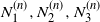 ${N_{1}^{(n)}},{N_{2}^{(n)}},{N_{3}^{(n)}}$
be independent Poisson processes with intensity
 $\gamma$
(and independent of everything else). It follows from (7) and
 $A_{n}=_{\rm d} {\textbf{\textit{N}}}_{\boldsymbol{\gamma}}(Z_{n})$
that
 $\mathcal{R}_{n}(A_n)$
has the same distribution as
 ${\textbf{\textit{N}}}_{\boldsymbol{\gamma}}(\mathcal{S}_n(Z_n))$
. Hence, there is a probability space on which
 $A_n$
and i.i.d.
 $(U_{n,k})_{k=1,2,\ldots}$
(with distribution necessarily equal to that of
 $\Theta$
) exist such that
 $\sum_{k=1}^{A_n}U_{n,k}={N_{1}^{(n)}}(\mathcal{S}_n(Z_n))$
almost surely. Let
 $C_n={N_{2}^{(n)}}(Y_n)$
and
 $W_n={N_{3}^{(n)}}((1-\lambda/\gamma)B_n)$
. Since
 \begin{align*}G_{W_n}(s)=\varphi_{B_n}\bigg(\bigg(1-\frac{\lambda}{\gamma}\bigg)\gamma s\bigg)=\frac{\lambda}{\lambda+\left(\gamma-\lambda\right) s}=\frac{\lambda/\gamma}{\lambda/\gamma+(1-\lambda/\gamma)s},\end{align*}
it follows that  $W_n=_{\rm d}\textrm{Geom}\!\left(\lambda/\gamma\right)$
as required. To complete the construction we define
 \begin{align*}A_{n+1}=({N_{1}^{(n)}}(\mathcal{S}_n(Z_n))+C_{n}-W_n)^{+}.\end{align*}
Then 2–4 are fulfilled and, applying (8), we see that  $A_{n+1}=_{\rm d} {\textbf{\textit{N}}}_{\boldsymbol{\gamma}}(Z_{n+1})$
, too.
As an example, suppose that  $\mathcal{S}_n(t)=at$
with
 $a\in [0, 1)$
, where the GAR+ process is given by
 \begin{align*}Z_{n+1}=(aZ_n+Y_n-B_n)^{+}, \qquad n \in \mathbb{N}_{0},\end{align*}
as studied in [Reference Boxma, Mandjes and Reed7]. Since  ${\textbf{\textit{N}}}_{\boldsymbol{\gamma}}(aX)=_{\rm d} a\circ {\textbf{\textit{N}}}_{\boldsymbol{\gamma}}(X)$
, it follows that the discrete counterpart is given by the INGAR+ process
 \begin{align*}A_{n+1}=\left(a\circ A_n+C_{n}-W_n\right)^{+}, \qquad n \in \mathbb{N}_{0},\end{align*}
a generalized INAR(1) process.
Remark 2. Note that not every integer-valued non-negative random variable appears as an image under the transformation  ${\textbf{\textit{N}}}_{\boldsymbol{\gamma}}$
. For example, every random variable
 ${\textbf{\textit{N}}}_{\boldsymbol{\gamma}}(X)$
with X non-negative has an infinite support, in fact
 $\mathbb{P}({\textbf{\textit{N}}}_{\boldsymbol{\gamma}}(X)=k)>0$
for every
 $k\in\mathbb{N}_{0}$
. It follows that there are INGAR+ processes which cannot be obtained as counterparts from a GAR+ process using the above construction. Hence, while it is possible to derive results for general GAR+ processes from those of the corresponding INGAR+ processes, the converse does not always work. In the forthcoming section we therefore first investigate INGAR+ processes, and in Section 4 apply these results to GAR+ processes via the duality.
3. The INGAR+ model
In this section we analyze the INGAR+ model, the main objective being to uniquely characterize its time-dependent and stationary behavior. Recall that the INGAR+ model is defined by the recursion
 \begin{align}A_{n+1}\coloneqq\left(\mathcal{R}_{n}({A_n})+C_{n}-W_n\right)^{+},\end{align}
with  $(\mathcal{R}_{n}(\cdot))_{n\in\mathbb{N}_{0}}$
,
 $(C_n)_{n\in\mathbb{N}_{0}}$
, and
 $(W_n)_{n\in\mathbb{N}_{0}}$
as introduced earlier; in particular,
 $W_n$
has a geometric distribution with success probability p. It requires a direct verification to see that the APGF of the random sum
 $\mathcal{R}_{n}(A_n)$
is given by
 $G_{A_n}(\Psi(s))$
, where
 $\Psi(s)\coloneqq 1-{G_{U}}(s)$
. The function
 $\Psi(\cdot)$
is increasing and concave with
 $\Psi(0)=0$
. We will make frequent use of the iterates
 \begin{align*}\Psi^{(0)}(s)=s,\quad \Psi^{(k)}(s)=\Psi(\Psi^{(k-1)}(s)),\qquad k=1,2,\ldots \end{align*}
The time-dependent behavior of  $A_n$
is studied in Section 3.1, and the stationary behavior in Section 3.2. Joint APGFs and moments are derived in Section 3.3.
3.1. Time-dependent analysis
A specific type of functional difference equation naturally appears in the analysis of the INGAR+ and GAR+ models. The following lemma gives a solution of this difference equation, for a sufficiently general setup. The proof is standard, in that it follows directly by iterating the equation (and is therefore omitted).
Lemma 1. Suppose that, for a given initial value  $f_0$
, a sequence of functions
 $f=(\kern2pt f_n)_{n\in\mathbb{N}_{0}}$
is defined by
 \begin{align}f_{n}(s)&=\pi(s)f_{n-1}(\Psi(s))-\varrho(s)f_{n-1}(\Psi(p))+\kappa,\qquad n\geq 1,\end{align}
for functions  $\pi(\cdot)$
and
 $\varrho(\cdot)$
and a constant
 $\kappa$
. Then
 \begin{align}f_{n}(s)&=f_{0}(\Psi^{(n)}(s))\prod_{i=0}^{n-1} \pi(\Psi^{(i)}(s))\nonumber\\[3pt] &\qquad +\kappa\sum_{i=0}^{n-1}\prod_{j=0}^{i-1} \pi(\Psi^{(j)}(s))-\sum_{i=1}^{n} f_{n-i}(\Psi(p))\varrho(\Psi^{(i-1)}(s))\prod_{j=0}^{i-2} \pi(\Psi^{(j)}(s)), \end{align}
for  $n\in \mathbb{N}_0$
. The values of
 $f_{j}(\Psi(p))$
follow recursively by inserting
 $s=\Psi(p)$
into (11).
We apply the above lemma in order to obtain the APGFs  $G_{A_n}(\cdot)$
,
 $n=1,2,\dots$
, when
 ${G_{A_0}(\cdot)}$
is given. Define
 \begin{align}\Pi_n(s)\coloneqq \prod_{k=0}^{n-1}\frac{pG_{C}(\Psi^{(k)}(s))}{p-\Psi^{(k)}(s)},\qquad\Gamma_n(s)\coloneqq \frac{\Psi^{(n)}(s)}{p-\Psi^{(n)}(s)} \,\Pi_n(s),\end{align}
with empty products to be defined equal to one. Whenever the infinite product  $\lim_{n\to\infty}\Pi_n(s)$
converges we simply write
 $\Pi_\infty(s)$
for its value. The following result provides the APGFs
 $G_{A_n}(\cdot)$
in terms of the functions
 $\Pi_n(\cdot)$
and
 $\Gamma_n(\cdot)$
featuring in (12).
Theorem 4. For  $n=0,1,\ldots$
and
 $s\in[0, 1]$
,
 \begin{align}G_{A_{n}}(s)&=G_{A_0}(\Psi^{(n)}(s))\,\Pi_{n}(s) -G_{C}(p)\sum_{j=0}^{n-1}G_{A_{{n-j-1}}}(\Psi(p))\,\Gamma_{j}(s).\end{align}
The values of  $G_{A_{n}}(\Psi(p))$
follow recursively by inserting
 $s=\Psi(p)$
into (13); see Remark 4.
Proof. By rearranging relation (A1) in the appendix, we obtain, from (9),
 \begin{align}G_{A_{n+1}}(s)&=\frac{p}{p-s}\,G_{\mathcal{R}_{n}(A_n)+C_n}(s)-\frac{s}{p-s}\,G_{\mathcal{R}_{n}(A_n)+C_n}(p)\nonumber\\[4pt] &=\underbrace{\frac{pG_{C}(s)}{p-s}}_{\pi(s)} G_{A_{n}}(\Psi(s))-\underbrace{\frac{sG_{C}(p)}{p-s}}_{\varrho(s)}G_{A_{n}}(\Psi(p)).\end{align}
This function is of the type (10) with  $\kappa = 0$
.
Remark 3. Since (13) is a consequence of the purely arithmetic Lemma 1, there are no issues in relation to convergence. Relation (13) is true for all  $s\in[0, 1]$
. Note that the first term of the difference on the right-hand side has the same singularities as the second term (which are the values s for which
 $p = \Psi^{(k)}(s)$
for some k). It can be verified that these singularities are removable; each singularity in the first term of the right-hand side of (13) is compensated by that same singularity in the second term of the right-hand side. In this respect, observe that
 $s=p$
is a removable singularity in (14).
Remark 4. Inserting  $s=\Psi(p)$
into (13) shows that
 \begin{align}G_{A_{n}}(\Psi(p))&=G_{A_0}(\Psi^{(n+1)}(p))\,\Pi_{n}(\Psi(p))-G_{C}(p)\sum_{j=0}^{n-1}G_{A_{n-j-1}}(\Psi(p))\,\Gamma_{j}(\Psi(p)).\end{align}
With this relation, the constants  $G_{A_{n}}(\Psi(p))$
can be found recursively.
3.2. Stationary analysis
Now we turn to the stationary analysis. In the analysis, an important role is played by  $\xi$
, denoting the limit as
 $n\to\infty$
of the probability that
 $\mathcal{R}_{n}(A_{n})+C_n-W_n$
is strictly smaller than zero, i.e.
 \begin{align*}\xi=\lim_{n\to \infty}\mathbb{P}\!\left(W_n> \mathcal{R}_{n}(A_{n})+C_n\right),\end{align*}
whenever it exists.
Theorem 5. If (S1) holds, then the INGAR+ process  $(A_n)_{n\in\mathbb{N}_{0}}$
is positive recurrent. The stationary APGF is given by
 \begin{align*}G_{A}(s)&=\Pi_\infty(s)-\xi\,\Sigma(s),\end{align*}
where  $\Sigma(s)\coloneqq\sum_{n=0}^\infty \Gamma_{n}(s)$
and
 \begin{align}\xi=G_{C}(p)\,G_{A}(\Psi(p))=\frac{G_{C}(p)\,\Pi_\infty(\Psi(p))}{1+G_{C}(p)\,\Sigma(\Psi(p))}.\end{align}
Proof. Let the process  $(A^{+}_n)_{n\in\mathbb{N}_{0}}$
be defined by
 $A^{+}_0=A_0$
and
 $A^{+}_{n+1}=\mathcal{R}_{n}(A^{+}_n)+C_n$
. Then
 $(A^{+}_n)_{n\in\mathbb{N}_{0}}$
is a Galton–Watson branching process with immigration. As follows from [Reference Heathcote14, Reference Heathcote15], under (S1) this process is positive recurrent and, since it majorizes
 $(A_n)_{n\in\mathbb{N}_{0}}$
, the same follows for our INGAR+ process.
To determine the APGF of the stationary distribution we use the generating functions
 \begin{align*}A(r,s)=\sum_{n=0}^\infty r^n G_{A_n}(s),\ B(r,s)=\sum_{n=0}^\infty r^n \beta_n(s),\ D(r,s)=\sum_{n=0}^\infty r^n \Gamma_n(s),\quad r\in(-1,1),\end{align*}
where  $\beta_n(s)\coloneqq\ G_{A_0}(\Psi^{(n)}(s))\,\Pi_{n}(s).$
It follows from (15) that
 \begin{align*}G_{A_{n}}(\Psi(p))&=\beta_n(\Psi(p))-G_{C}(p)\sum_{j=0}^{n-1}G_{A_{n-j-1}}(\Psi(p))\,\Gamma_j(\Psi(p)),\end{align*}
and hence, after standard algebraic manipulations,
 \begin{align*}A(r,\Psi(p))=\frac{B(r,\Psi(p))}{1+G_{C}(p)\,rD(r,\Psi(p))}.\end{align*}
Under condition (S1) we have  $\mathbb{E}(U)<1$
and
 $\Psi^{(n)}(s)=O(\mathbb{E}(U)^n)\downarrow 0$
as
 $n\to\infty$
; see [Reference Athreya and Ney3, Theorem 11.1]. It follows that the product
 \begin{equation*}\prod_{k=0}^{n-1}\frac{p}{p-\Psi^{(k)}(s)}\end{equation*}
tends to a finite non-zero limit as  $n\to\infty$
. Moreover,
 $\prod_{k=0}^{\infty}G_{C}(\Psi^{(k)}(s))$
is the LST of the limit distribution of the Galton–Watson process
 $(A^{+}_n)_{n\in\mathbb{N}_{0}}$
; see, e.g., [Reference Heathcote14]. Hence,
 $\beta_n(s)$
tends to a finite non-zero limit
 $\Pi_\infty(s)$
. The convergence of
 $\beta_n$
together with
 $\Psi^{(n)}(s)=O((\mathbb{E}(U))^n)\downarrow 0$
implies the convergence of
 $\sum_{k=0}^n \Gamma_k(s)$
to
 $\Sigma(\Psi(s))$
as
 $n\to\infty$
. Hence, using Abel’s theorem, we obtain
 \begin{align*}G_{A}(\Psi(p))&=\lim_{r\uparrow 1}(1-r)A(r,\Psi(p))=\frac{\displaystyle \lim_{r\uparrow 1}(1-r)B(r,\Psi(p))}{\displaystyle 1+G_{C}(p)\lim_{r\uparrow 1}rD(r,\Psi(p))}=\frac{\Pi_\infty(\Psi(p))}{1+G_{C}(p)\,\Sigma(\Psi(p))},\end{align*}
and
 \begin{align*}G_{A}(s)&=\lim_{r\uparrow 1}(1-r)A(r,s)=\lim_{r\uparrow 1}(1-r)\;B(r,s)-\lim_{r\uparrow 1}\;(1-r)G_{C}(p) D(r,s)A(r,\Psi(p))\\[3pt] &=\Pi_\infty(s)-G_{A}\,(\Psi(p))\,G_{C}(p)\,\Sigma(s).\end{align*}
It remains to prove that  $\xi_n= \mathbb{P}(W_n> \mathcal{R}_{n}(A_{n})+C_n)$
indeed converges to
 $G_{C}(p)G_{A}(\Psi(p))$
as
 $n\to\infty$
. According to (A2) in the appendix and the recurrence relation (9) we obtain
 \begin{align*}\xi_n &=G_{\mathcal{R}_{n}(A_{n})+C_n}(p)=G_{C}(p)\,G_{A_n}(\Psi(p)).\end{align*}
Claim (16) thus follows by sending n to  $\infty$
.
Remark 5. Condition (S1) is clearly not necessary in the case where  $U\equiv 1$
. In this case the INGAR+ process
 $A_{n+1}=\left(A_n+C_{n}-W_n\right)^{+}$
is a reflected random walk and, as is well known,
 $\mathbb{E}(C)<\mathbb{E}(W)$
ensures positive recurrence. However, it is not obvious how necessary conditions can be derived in the general INGAR+/GAR+ setting. To illustrate the complications one encounters in studying the
 $\mathbb{E}(U)=1$
case, assume that, additionally,
 $\textrm{Var}\!\left(U\right)<\infty$
. One can show that in this case
 $\Psi^{(k)}(s)\sim 1/k$
as
 $k\to\infty$
; see [Reference Athreya and Ney3, Theorem 11.1]. This implies that both main terms in (13), i.e.
 \begin{align*}&G_{A_0}(\Psi^{(n)}(s))\,\Pi_n(s)\:\:\:\mbox{and}\:\:\:G_{C}(p)\sum_{j=0}^{n-1}G_{A_{n-j-1}}(\Psi(p))\,\Gamma_n(s),\end{align*}
tend to infinity as  $n\to\infty$
. It follows that it is not clear whether their difference tends to zero, tends to a finite non-zero limit, or does not converge at all.
Remark 6. In passing, we have also shown that
 \begin{equation*}A(r,s)= B(r,s)-G_{C}(p)\,A(r,\Psi(p))\,rD(r,s) = B(r,s)-G_{C}(p)\frac{B(r,\Psi(p))\,rD(r,s)}{1+G_{C}(p)\,rD(r,\Psi(p))},\end{equation*}
as revealed by the proof of Theorem 5.
In the case  $A_0=\ell$
, we have that B(r, s) equals
 $B(r,s\,|\,\ell)$
, given by
 \begin{equation*} B(r,s\,|\,\ell)\coloneqq \sum_{n=0}^\infty r^n \big(1-\Psi^{(n)}(s)\big)^\ell \Pi_n(s).\end{equation*}
The fact that this is a power in  $\ell$
will be exploited in the proof of Theorem 9.
3.3. Moments and covariance structure
In this subsection we include various results concerning the moments and covariance structure of the INGAR+ process  $({A_n})_{n\in\mathbb{N}_{0}}$
. As before,
 $\xi_n$
is defined by
 $\mathbb{P}(W_n> \mathcal{R}_{n}(A_{n})+C_n)$
, which we have seen to equal
 $G_{C}(p)\,G_{A_n}(\Psi(p)).$
Theorem 6. The mean and the variance of the INGAR+ process fulfil the following recursions:
 \begin{align}\hspace*{-30pt}\mathbb{E}\!\left(A_{n+1}\right)& = \mathbb{E}\!\left(U\right)\mathbb{E}\!\left(A_n\right)+\mathbb{E}\!\left(C\right)-\frac{1-\xi_n}{p},\hspace*{50pt}\end{align}
 \begin{align}\textrm{Var}\!\left(A_{n+1}\right)& = \textrm{Var}\!\left(A_n\right)\mathbb{E}\!\left(U\right)^2+\mathbb{E}\!\left(A_n\right)\textrm{Var}\!\left(U\right)+\textrm{Var}\!\left(C\right)\nonumber\\[3pt] &\quad -\frac{2\xi_n}{p}\left(\mathbb{E}\!\left(A_n\right)\mathbb{E}\!\left(U\right)+\mathbb{E}\!\left(C\right)\right)+\frac{(1-\xi_n)(1-p+\xi_n)}{p^2}. \end{align}
In stationarity,
 \begin{align}\mathbb{E}\!\left(A\right) & = \frac{\mathbb{E}\!\left(C\right)-{\displaystyle \frac{1-\xi}{p}}}{1-\mathbb{E}\!\left(U\right)},\end{align}
 \begin{align}\textrm{Var}\!\left(A\right)& = \frac{\mathbb{E}\!\left(A\right)\textrm{Var}\!\left(U\right)+\textrm{Var}\!\left(C\right)-{\displaystyle \frac{2\xi}{p}}\left(\mathbb{E}\!\left(A\right)\mathbb{E}\!\left(U\right)+\mathbb{E}\!\left(C\right)\right)+{\displaystyle \frac{(1-\xi)(1-p+\xi)}{p^2}}}{1-(\mathbb{E}\!\left(U\right)\!)^2}.\end{align}
Proof. We start by multiplying (14) by  $p-s$
; recalling that
 $\xi_n=G_{\mathcal{R}_{n}(A_{n})+C_n}(p)$
, we obtain, by differentiating with respect to s,
 \begin{align}-G_{A_{n+1}}(s)+(p-s)G^{\prime}_{A_{n+1}}(s)=pG^{\prime}_{C}(s) G_{A_{n}}(\Psi(s))+pG_{C}(s) G^{\prime}_{A_{n}}(\Psi(s))\Psi^{\prime}(s)-\xi_n.\end{align}
Letting  $s\to 0$
we obtain
 \begin{align*}-1-p\mathbb{E}\!\left(A_{n+1}\right)&=-p\mathbb{E}\!\left(C\right) -p \mathbb{E}\!\left(A_n\right)\mathbb{E}\!\left(U\right)-\xi_n,\end{align*}
from which (17) follows. Moreover, taking another derivative in (21) and letting  $s\to 0$
we obtain
 \begin{align*}p\big(\mathbb{E}(A_{n+1}^2)-\mathbb{E}(A_{n+1})\big)+2\mathbb{E}\!\left(A_{n+1}\right)&= p\big(\mathbb{E}(C^2)-\mathbb{E}(C)\big)+2p\mathbb{E}\!\left(C\right)\mathbb{E}\!\left(A_n\right)\mathbb{E}\!\left(U\right) \\[3pt] &\quad + p\big(\mathbb{E}(A_n^2)-\mathbb{E}(A_n)\big)\mathbb{E}\!\left(U\right)^2- p\mathbb{E}\!\left(A_n\right)\big(\mathbb{E}(U)-\mathbb{E}(U^2)\big),\end{align*}
which leads to (18). The stationary mean (19) and variance (20) follow by letting n tend to infinity and solving  $\mathbb{E}(A)$
and
 $\textrm{Var}(A)$
, respectively.
Besides the mean and variance of  $A_n$
, we can use similar techniques to obtain insight into the process’ correlation structure. Our next objective is to evaluate the joint APGF of
 $A_n$
and
 $A_{n+1}$
. This joint APGF
 $G_{A_n,A_{n+1}}(s,t)$
is expressed in terms of the (univariate) APGF of
 $A_n$
, which is given by Theorem 4. We restrict ourselves to
 $t \neq p$
; the result for
 $t=p$
follows in an elementary way by taking a limit.
Theorem 7. For  $t\not=p$
,
 \begin{align}G_{A_n,A_{n+1}}(s,t)&=\frac{p}{p-t}\,G_{C}(t)\,G_{A_n}(1-(1-s)G_{U}(t))\nonumber\\[3pt] &\quad -\frac{t}{p-t}\,G_{C}(p)\,G_{A_n}(1-(1-s)G_{U}(p)). \end{align}
Proof. By conditioning, we obtain
 \begin{align*}G_{A_n,A_{n+1}}(s,t)&=\mathbb{E}\big((1-s)^{A_n}(1-t)^{\left(\mathcal{R}_{n}(A_n)+C_{n}-W_n\right)^{+}}\big)\\[3pt] &=\mathbb{E}\Big((1-s)^{A_n}\mathbb{E}\big((1-t)^{\left(\mathcal{R}_{n}(A_n)+C_{n}-W_n\right)^{+}} \mid \mathcal{R}_{n}(A_n),C_n\big)\Big).\end{align*}
By (A1) in the appendix it follows that, for every  $k\in\mathbb{N}_{0}$
, provided that
 $p\not=t$
,
 \begin{align*}\mathbb{E}\big((1-t)^{(k-W_n)^{+}}\big)=\frac{p}{p-t}(1-t)^{k}-\frac{t}{p-t}(1-p)^k.\end{align*}
Hence, for  $p\not=t$
,
 \begin{align*}\mathbb{E}\Big((1-&s)^{A_n}\mathbb{E}\big((1-t)^{\left(\mathcal{R}_{n}(A_n)+C_{n}-W_n\right)^{+}} \mid \mathcal{R}_{n}(A_n),C_n\big)\Big)\\[3pt] &=\mathbb{E}\big((1-s)^{A_n}\frac{p}{p-t}(1-t)^{\mathcal{R}_{n}(A_n)+C_{n}}-(1-s)^{A_n}\frac{t}{p-t}(1-p)^{\mathcal{R}_{n}(A_n)+C_{n}}\big)\\[3pt] &=\frac{p}{p-t}G_{C}(t)\,G_{A}\big(1-(1-s)G_{U}(t)\big)-\frac{t}{p-t}G_{C}(p)\,G_{A}\big(1-(1-s)G_{U}(p)\big),\end{align*}
where we used the fact that
 \begin{align*}\mathbb{E}\big((1-s)^A(1-t)^{\mathcal{R}(A)}\big)&=\mathbb{E}\big((1-s)^A\mathbb{E}\big((1-t)^{\mathcal{R}(A)} \mid A\big)\big)=\mathbb{E}\big((1-s)^AG_{U}(t)^A\big)\\[3pt] &=G_{A}(1-(1-s)\,G_{U}(t)).\end{align*}
□
Theorem 8. The covariance of  $A_n$
and
 $A_{n+1}$
is given by
 \begin{align}&\textrm{Cov}\!\left({A_n},{A_{n+1}}\right)=\mathbb{E}\!\left(U\right)\textrm{Var}\!\left(A_n\right)-\frac{\xi_n}{p}\mathbb{E}\!\left(A_n\right)-\frac{1}{p}G_{C}(p)G_{U}(p)G^{\prime}_{A_n}(\Psi(p)).\end{align}
Proof. To derive an expression for  $\mathbb{E}(A_n\,A_{n+1})$
, we first take the derivative of (22) with respect to s, to obtain
 \begin{align*}\frac{\partial}{\partial s}G_{A_n,A_{n+1}}(s,t)&=\frac{p}{p-t}G_{C}(t)G^{\prime}_{A_n}(1-(1-s)G_{U}(t))\,G_{U}(t)\nonumber\\[3pt] &\quad +\Big(1-\frac{p}{p-t}\Big)G_{C}(p)G^{\prime}_{A_n}(1-(1-s)G_{U}(p))\,G_{U}(p).\end{align*}
Then, taking the derivative with respect to t yields
 \begin{align*}\frac{\partial^2}{\partial t\partial s}G_{A_n,A_{n+1}}(s,t)&=\frac{p}{(p-t)^2}G_{C}(t)\,G^{\prime}_{A_n}(1-(1-s)G_{U}(t))\,G_{U}(t)\\[3pt] &\quad +\frac{p}{p-t}G^{\prime}_{C}(t)\,G^{\prime}_{A_n}(1-(1-s)G_{U}(t))\,G_{U}(t)\\[3pt] &\quad-(1-s)\frac{p}{p-t}G_{C}(t)G^{\prime\prime}_{A_n}(1-(1-s)G_{U}(t))G^{\prime}_{U}(t)\,G_{U}(t)\\[3pt] &\quad +\frac{p}{p-t}G_{C}(t)\,G^{\prime}_{A_n}(1-(1-s)G_{U}(t))\,G^{\prime}_{U}(t)\\[3pt] &\quad -\frac{p}{(p-t)^2 }\,G_{C}(p)\,G^{\prime}_{A_n}(1-(1-s)G_{U}(p))\,G_{U}(p).\end{align*}
Letting  $s\downarrow 0$
and
 $t\downarrow 0$
we obtain
 \begin{align*}\mathbb{E}\!\left(A_n\,A_{n+1}\right)&=\mathbb{E}\!\left(A_n\right)\bigg(\mathbb{E}\!\left(C\right)-\frac{1}{p}\bigg)+\mathbb{E}\big(A_n^2\big)\mathbb{E}\!\left(U\right) -\frac{G_{C}(p)\,G^{\prime}_{A_n}(\Psi(p))\,G_{U}(p)}{p}. \end{align*}
Then,
 \begin{align*}\textrm{Cov}\!\left({A_n},{A_{n+1}}\right)=&\,\mathbb{E}\!\left(U\right)\mathbb{E}\big(A_n^2\big)+\mathbb{E}\!\left(A_n\right)\left(\mathbb{E}\!\left(C\right)-\frac{1}{p}\right)-\frac{1}{p}G_{C}(p)\,G_{U}(p)\,G^{\prime}_{A_n}(\Psi(p))\\[3pt] &-\mathbb{E}\!\left(A_n\right)\bigg(\mathbb{E}\!\left(A_n\right)\mathbb{E}\!\left(U\right)+\mathbb{E}\!\left(C\right)-\frac{1-\xi_n}{p}\bigg),\end{align*}
which can be checked to equal the right-hand side of (23).
We conclude this section by presenting the joint APGF of  $A_0$
and
 $A_N$
, where N is geometrically distributed, i.e.
 $\mathbb{P}(N=n) = r^n(1-r)$
for
 $n\in\mathbb{N}_0$
and
 $r\in[0, 1]$
. We assume that the process is stationary, i.e.
 $A_0$
has the stationary distribution characterized in Theorem 5 (which, evidently, also implies that
 $A_N$
follows the stationary distribution). This joint APGF, which can be seen as the discrete r-transform of the joint APGF of
 $A_0$
and
 $A_n$
(with
 $n\in\mathbb{N}_0$
), provides insight into the level of correlation within the INGAR+ process; in particular, by differentiation it allows the computation of the r-transform of the covariance between
 $A_0$
and
 $A_n$
. The results obtained may open the opportunity to get insight into structural properties of
 $\textrm{Cov}({A_0},{A_n})$
; cf. similar results for Lévy-fed queues [Reference Berkelmans, Cichocka and Mandjes6, Reference Glynn and Mandjes12]. Combining the above results, we obtain a representation for
 $G_{A_0,A_N}(t,s)=\mathbb{E}((1-t)^{A_0}(1-s)^{A_N})$
, as follows. First, observe that
 \begin{align*} G_{A_0,A_N}(t,s) &= (1-r)\sum_{n=0}^\infty r^n \sum_{\ell=0}^\infty \mathbb{E}((1-t)^{A_0}(1-s)^{A_n}\,|\,A_0=\ell)\,\mathbb{P}\!\left(A_0=\ell\right)\\[3pt] &= (1-r)\sum_{n=0}^\infty r^n \sum_{\ell=0}^\infty (1-t)^{\ell}G_{A_n}(s\,|\,\ell)\,\mathbb{P}\!\left(A_0=\ell\right),\end{align*}
where  $G_{A_n}(s\,|\,\ell)\coloneqq\mathbb{E}((1-s)^{A_n}\,|\,A_0=\ell)$
. Relying on Remark 6, and remarking that in A(r, s) only B(r, s) depends on the distribution of
 $A_0$
,
 \begin{align*}\sum_{n=0}^\infty r^n G_{A_n}(s\,|\,\ell) &= \sum_{n=0}^\infty r^n \big(1-\Psi^{(n)}(s)\big)^\ell \Pi_n(s) \\[3pt] & \quad - \frac{G_{C}(p)\,rD(r,s)}{1+G_{C}(p)\,rD(r,\Psi(p))}\sum_{n=0}^\infty r^n \big(1-\Psi^{(n+1)}(p)\big)^\ell \Pi_n(\Psi(p)).\end{align*}
Combining the above elements, and using that  $A_0$
obeys the equilibrium distribution, we arrive, after some algebra, at the following result.
Theorem 9. The joint APGF of  $A_0$
and
 $A_N$
(in stationarity) is given, with
 $G_A(\cdot)$
as determined in Theorem 5, by
 \begin{align*}&G_{A_0,A_N}(t,s)= (1-r)\sum_{n=0}^{\infty} r^n G_A\big(t +\Psi^{(n)}(s) -t \Psi^{(n)}(s)\big) \,\Pi_n(s) \\[3pt] &\quad - (1-r)\frac{G_{C}(p)\,rD(r,s)}{1+G_{C}(p)\,rD(r,\Psi(p))}\sum_{n=0}^\infty r^nG_A\big(t +\Psi^{(n+1)}(p) -t \Psi^{(n+1)}(p)\big) \,\Pi_n(\Psi(p)). \end{align*}
4. The GAR+ model
In this section we investigate the GAR+ model as specified in Section 1:
 \begin{align*} Z_{n+1}=\left(\mathcal{S}_n(Z_n)+Y_{n}-B_n\right)^{+},\end{align*}
with the random objects  $(\mathcal{S}_n(\cdot))_{n\in\mathbb{N}_{0}}$
,
 $(B_n)_{n\in\mathbb{N}_{0}}$
, and
 $(Y_n)_{n\in\mathbb{N}_{0}}$
as introduced earlier; in particular, we have
 $\mathbb{P}(B_n\le x)=1-e^{-\lambda x}$
for
 $x\ge 0$
. Recall that
 $(\mathcal{S}(t))_{t\in \mathbb{R}^{+}}$
is a Lévy subordinator with Laplace exponent
 $\psi$
.
This section has the same structure as the previous one, but, as it will turn out, we will greatly benefit from the the duality property that was described in Section 2, facilitating direct translation of the INGAR+ results into their GAR+ counterparts. The time-dependent behavior of  $Z_n$
is addressed in Section 4.1, while the stationary behavior is covered by Section 4.2; joint LSTs and moments are derived in Section 4.3. While our approach heavily relies on the duality, it is of course also possible to derive the results for GAR+ from scratch, by an iterative approach similar to the one we developed to analyze the INGAR+ model.
4.1. Time-dependent analysis
By Theorem 3 there is a dual INGAR+ process
 \begin{align*}A_{n+1}=\left(\mathcal{R}_{n}({A_n})+C_{n}-W_n\right)^{+},\end{align*}
when choosing
 \begin{align*}&A_n=_{\rm d} {\textbf{\textit{N}}}_{\boldsymbol{\gamma}}(Z_n),&\mathcal{R}_{n}(A_n) & =_{\rm d} {\textbf{\textit{N}}}_{\boldsymbol{\gamma}}(\mathcal{S}_n(Z_n)) \quad\text{(i.e.}\ U_{n,k} =_{\rm d} \Theta\text{)},\\[3pt] &C_n=_{\rm d} {\textbf{\textit{N}}}_{\boldsymbol{\gamma}}(Y_n),&W_n & =_{\rm d} \mbox{Geom}(p).\end{align*}
This identification enables us to translate INGAR+ results to their GAR+ counterparts, as we will show below. Since  $\varphi_{Z_n}(s)=G_{A_n}(\gamma s)$
by (3), we can express the results for generating functions in terms of Laplace transforms. Also, note that
 $\Psi(s)=1-G_{U}(s)=\psi(\gamma s)/\gamma$
and it follows that
 $\psi^{(k)}(s)=\gamma\Psi^{(k)}(s/\gamma)$
and
 $\Psi^{(k)}(s)=\psi^{(k)}(\gamma s)/\gamma$
. Define
 \begin{equation*}\Pi^{\ast}_n(s)\coloneqq\prod_{k=0}^{n-1}\frac{\lambda\varphi_{Y}(\psi^{(k)}(s))}{\lambda-\psi^{(k)}(s)} , \qquad \Gamma^\ast_n(s)\coloneqq\frac{\psi^{(n)}(s)}{\lambda-\psi^{(n)}(s)}\,\Pi^{\ast}_n(s).\end{equation*}
The following theorem immediately follows from the duality relations of Section 2 (see, in particular, Theorem 3) and Theorem 4.
Theorem 10. For  $n=0,1,\ldots$
and
 $s\in[0, 1]$
,
 \begin{align}\varphi_{Z_{n}}(s)&=\varphi_{Z_0}(\psi^{(n)}(s))\,\Pi^{\ast}_n(s)-\varphi_{Y}(\lambda)\sum_{j=0}^{n-1}\varphi_{Z_{n-j-1}}(\psi(\lambda))\,\Gamma^\ast_j(s).\end{align}
The values of  $\varphi_{Z_{n}}(\psi(\lambda))$
follow recursively by inserting
 $s=\psi(\lambda)$
into (24).
4.2. Stationary analysis
Regarding the stationary behavior, we will mimic Theorem 5. First, we show that the stability conditions (S1) and (S2) are equivalent here, if  $A_n$
,
 $\mathcal{R}_{n}(A_n)$
,
 $C_n$
, and
 $W_n$
are as defined above.
Proof. Since  $U=_{\rm d}\Theta=_{\rm d} \mathcal{S}(1)$
we have that
 $\mathbb{E}(U)<1$
is equivalent to
 $\mathbb{E}(\mathcal{S}(1))<1$
. Moreover, using integration by parts,
 \begin{align}\mathbb{E}\!\left(\log(1+Y)\right)=\int_0^\infty \log(1+y)\,\mathbb{P}\!\left(Y\in {\rm d}y\right)=\int_0^\infty \frac{1}{1+y}\mathbb{P}\!\left(Y>y\right)\,{\rm d}y.\end{align}
Note that, for any given  $\varepsilon>0$
,
 \begin{align*}\frac{1}{1+y}\sim \frac{1-{\rm e}^{-\varepsilon y}}{y} \end{align*}
as  $y\to\infty$
. Hence, the integral on the right-hand side of (25) is finite if and only if
 \begin{align*}\int_0^\infty \frac{1-{\rm e}^{-\varepsilon y}}{y}\mathbb{P}\!\left(Y>y\right)\,{\rm d}y=\int_0^\varepsilon \frac{1-\varphi_ Y(s)}{s}\,{\rm d}s\end{align*}
is finite for some  $\varepsilon>0$
(where the last equality is a consequence of the observation that
 ${(1 - {\rm e}^{-\varepsilon y})}/{y} = \int_0^{\varepsilon} {\rm e}^{-sy} \,{\rm d}s$
). This finiteness condition is, by our duality, equivalent to
 \begin{equation*}\int_0^\varepsilon \frac 1 s \left(1-G_ C(s)\right) {\rm d}s<\infty\end{equation*}
for some  $\varepsilon>0$
. But, due to [Reference Heathcote15], this condition is equivalent to
 $\mathbb{E}(\log 1+C)<\infty$
.
The following theorem immediately follows from the duality relations of Section 2 (see, in particular, Corollary 3) and Theorem 5.
Theorem 11. If (S2) holds then the GAR+ process  $(Z_n)_{n\in\mathbb{N}_{0}}$
is positive recurrent. The limit stationary LST is given by
 \begin{align*}\varphi_{Z}(s)&=\Pi^{\ast}_\infty(s)-\eta\Sigma^\ast(s),\end{align*}
where  $\Sigma^\ast(s)\coloneqq\sum_{n=0}^\infty\Gamma^\ast_n(s)$
and
 \begin{align*}\eta=\mathbb{P}\!\left(Z=0\right)=\varphi_{Y}(\lambda)\varphi_{Z}(\psi(\lambda))=\frac{\varphi_{Y}(\lambda)\Pi^{\ast}_\infty(\psi(\lambda))}{1+\varphi_{Y}(\lambda)\Sigma^\ast(\psi(\lambda))}. \end{align*}
4.3. Moments and covariance structure
In this subsection we focus on deriving explicit formulas for moments and joint LSTs.
Theorem 12. The mean and the variance of the GAR+ process fulfil the following recursions:
 \begin{align*}\mathbb{E}\!\left(Z_{n+1}\right)& = \mathbb{E}\!\left(\mathcal{S}(1)\right)\mathbb{E}\!\left(Z_n\right)+\mathbb{E}\!\left(Y\right)-\frac{1-\eta_n}{\lambda}, \\[3pt] \textrm{Var}\!\left(Z_{n+1}\right)& = \textrm{Var}\!\left(Z_n\right)\mathbb{E}\!\left(\mathcal{S}(1)\right)^2+\mathbb{E}\!\left(Z_n\right)\textrm{Var}\!\left(\mathcal{S}(1)\right)+\textrm{Var}\!\left(Y\right) \\[3pt] & \quad - \frac{2\eta_n }{\lambda}\left(\mathbb{E}\!\left(Z_n\right)\mathbb{E}\!\left(\mathcal{S}(1)\right)+\mathbb{E}\!\left(Y\right)\right)+\frac{(1-\eta_n)(1+\eta_n)}{\lambda^2}, \end{align*}
where  $\eta_n=\mathbb{P}(Z_{n+1}=0)=\mathbb{P}(B_n>\mathcal{S}_n(Z_n)+Y_n)=\varphi_{Y}(\lambda)\varphi_{Z_n}(\psi(\lambda))$
. In stationarity,
 \begin{align*}\mathbb{E}\!\left(Z\right) & = \frac{\mathbb{E}\!\left(Y\right)-{\displaystyle \frac{1-\eta}{\lambda}}}{1-\mathbb{E}\!\left(\mathcal{S}(1)\right)},\\[3pt] \textrm{Var}\!\left(Z\right) & = \frac{\mathbb{E}\!\left(Z\right)\textrm{Var}\!\left(\mathcal{S}(1)\right)+\textrm{Var}\!\left(Y\right)-{\displaystyle \frac{2\eta }{\lambda}}\left(\mathbb{E}\!\left(Z\right)\mathbb{E}\!\left(\mathcal{S}(1)\right)+\mathbb{E}\!\left(Y\right)\right)+{\displaystyle \frac{(1-\eta)(1+\eta)}{\lambda^2}}}{1-\mathbb{E}\!\left(\mathcal{S}(1)\right)^2}.\end{align*}
Proof. Just translate Theorem 6 via the duality. Note that
 \begin{align*}\mathbb{E}\!\left(A_n\right) & = \gamma\mathbb{E}\!\left(Z_n\right), & \mathbb{E}\!\left(C\right) & = \gamma \mathbb{E}\!\left(Y\right),\\[3pt] \textrm{Var}\!\left(A_n\right) & = \gamma^2\textrm{Var}\!\left(Z_n\right)+\gamma\mathbb{E}\!\left(Z_n\right), & \textrm{Var}\!\left(C_n\right) & = \gamma^2\textrm{Var}\!\left(Y_n\right)+\gamma\mathbb{E}\!\left(Y_n\right),\\[3pt] \mathbb{E}\!\left(U\right) & = \mathbb{E}\!\left(\mathcal{S}(1)\right), & \textrm{Var}\!\left(U\right) & = \mathbb{E}\!\left(\mathcal{S}(1)\right)+\gamma\textrm{Var}\!\left(\mathcal{S}(1)\right)-\mathbb{E}\!\left(\mathcal{S}(1)\right)^2.\end{align*}
Moreover, since  $\lambda=\gamma p$
and
 $\psi(\gamma p)/\gamma =\Psi(p)$
, we have
 \begin{align*}\hspace*{82pt}\eta_n&=\varphi_{Y_n}(\lambda)\varphi_{Z_n}(\psi(\lambda))=G_{C_n}(p)G_{A_n}(\psi(\gamma p)/\gamma)=\xi_n. \hspace*{76pt}\square \end{align*}
We continue by discussing various results concerning the correlation structure of the  $(Z_n)_{n\in\mathbb{N}_{0}}$
process. We start by evaluating the joint LST of
 $Z_n$
and
 $Z_{n+1}$
, expressing it as
 $\varphi_{Z_n,Z_{n+1}}(s,t)$
in terms of the (univariate) LST of
 $Z_n$
, which is characterized through Theorem 5. We only cover the case
 $t\not=\lambda$
; if
 $t=\lambda$
the result follows by L’Hôpital’s rule.
Theorem 13. For  $t\not=\lambda$
,
 \begin{align}\varphi_{Z_n,Z_{n+1}}(s,t) = \frac{\lambda }{\lambda-t}\varphi_{Y}(t)\varphi_{Z_n}(s+\psi(t))-\frac{t}{\lambda-t}\varphi_{Y}(\lambda)\varphi_{Z_n}(s+\psi(\lambda)).\end{align}
Proof. By conditioning, we obtain
 \begin{align*}G_{Z_n,Z_{n+1}}(s,t)& = \mathbb{E}\big({\rm e}^{-sZ_n}{\rm e}^{-t\left(\mathcal{S}_n(Z_n)+Y_{n}-B_n\right)^{+}}\big) \\[3pt] & = \mathbb{E}\Big({\rm e}^{-sZ_n}\mathbb{E}\big({\rm e}^{-t\left(\mathcal{S}_n(Z_n)+Y_{n}-B_n\right)^{+}}\,|\,Y_n,\mathcal{S}_n(Z_n)\big)\Big).\end{align*}
By (A3), for every  $z\in\mathbb{R}$
,
 \begin{align*}\varphi_{(z-B)^{+}}(t)= \frac{\lambda {\rm e}^{-tz}- t {\rm e}^{-\lambda z}}{\lambda-t}{\rm e}^{-tz},\qquad \lambda\not=t,\end{align*}
so that
 \begin{align}\nonumber\mathbb{E}\Big({\rm e}^{-sZ_n}&\mathbb{E}\big({\rm e}^{-t\left(\mathcal{S}_n(Z_n)+Y_{n}-B_n\right)^{+}}\,|\,Y_n,\mathcal{S}_n(Z_n)\big)\Big) \\[3pt] & = \mathbb{E}\bigg(\frac{\lambda {\rm e}^{-sZ_n-t(\mathcal{S}_n(Z_n)+Y_n)} - t{\rm e}^{-sZ_n-\lambda(\mathcal{S}_n(Z_n)+Y_n)}}{\lambda-t}\bigg) \nonumber \\[3pt] & = \frac{\lambda}{\lambda-t}\varphi_{Y}(t)\,\mathbb{E}\Big({\rm e}^{-sZ_n-t\mathcal{S}_n(Z_n)}\Big)-\frac{t}{\lambda-t}\varphi_{Y}(\lambda)\,\mathbb{E}\!\left({\rm e}^{{-sZ_n-\lambda (\mathcal{S}_n(Z_n))}}\right).\end{align}
By the definition of  $\psi(\cdot)$
,
 \begin{align*}\mathbb{E}({\rm e}^{-s\mathcal{S}(X)})= \int_0^\infty {\rm e}^{-\psi(s)x}\,\mathbb{P}\!\left(X\in {\rm d}x\right)=\varphi_{X}(\psi(s)),\end{align*}
and
 \begin{align*}\mathbb{E}\Big({\rm e}^{-sZ_n-t\mathcal{S}_n(Z_n)}\Big)=\mathbb{E}\Big(\mathbb{E}\big({\rm e}^{-sZ_n-t\mathcal{S}_n(Z_n)} \mid Z_n\big)\Big)=\mathbb{E}\Big({\rm e}^{-sZ_n-\psi(t)Z_n}\Big)=\varphi_{Z_n}(s+\psi(t)).\end{align*}
Now some elementary algebra shows that (27) equals (26), as desired.
Theorem 14. The covariance of  $Z_n$
and
 $Z_{n+1}$
is given by
 \begin{align*}\textrm{Cov}\!\left({Z_n},{Z_{n+1}}\right)&=\mathbb{E}\!\left(\mathcal{S}(1)\right)\textrm{Var}\!\left(Z_n\right)-\frac{\eta_n}{\lambda}\mathbb{E}\!\left(Z_n\right)-\frac{\varphi_{Y}(\lambda)}{\lambda}\varphi^{\prime}_{Z_n}(\psi(\lambda)).\end{align*}
Proof. Note that the supposed straightforward approach via the duality and using the relation (6), which leads to  $\textrm{Cov}({A_n},{A_{n+1}})=\gamma^2\,\textrm{Cov}({{\textbf{\textit{N}}}_{\boldsymbol{\gamma}}(A_n)},{{\textbf{\textit{N}}}_{\boldsymbol{\gamma}}(A_{n+1})})$
, would yield a wrong result since a simple transformation
 $(A_n,A_{n+1})\mapsto({\textbf{\textit{N}}}_{\boldsymbol{\gamma}}(A_n),{\textbf{\textit{N}}}_{\boldsymbol{\gamma}}(A_{n+1}))$
does not preserve the dependence structure of the INGAR+ process. Instead, we used Theorem 13 and direct computations, analogous to those underlying Theorem 8.
The joint LST of  $Z_0$
and
 $Z_N$
, with N being geometrically distributed and the process being in equilibrium at time 0, can also be computed. As this amounts to paralleling the approach underlying Theorem 9, we omit this result.
5. Conclusion and suggestions for further research
We have introduced and analyzed two general classes of reflected autoregressive processes, INGAR+ and GAR+. In our approach a crucial role is played by a powerful duality relation that connects both classes of processes. We have shown that, despite the models’ general nature, a detailed analysis of the time-dependent and stationary behavior is possible. We started by analyzing the INGAR+ process, and subsequently we have used the duality relation to obtain the analogous results for the GAR+ process.
Various options for follow-up research arise. In this study the focus was primarily on transforms and moments, but one may wonder whether, in asymptotic regimes, the (time-dependent or stationary) distribution function can be explicitly given. The results in [Reference Boxma, Mandjes and Reed7] suggest potential scaling limits when approaching the stability limit (i.e.  $\mathbb{E}(U)\uparrow 1$
and
 $\mathbb{E}(\mathcal{S}(1))\uparrow 1$
for the INGAR+ and GAR+ model, respectively). In addition, one could try to derive the system’s tail behavior from the corresponding transforms; e.g. in the regime with heavy-tailed jumps in the upward direction, Tauberian techniques could be applied. We also aim to investigate some generalizations of the INGAR+ and GAR+ processes, allowing distributions for
 $W_n$
and
 $B_n$
that are more general than just the geometric and exponential distributions, respectively.
Other opportunities for future study concern multivariate extensions of the processes that we introduced. Such vector-valued counterparts are anticipated to be highly challenging, as for such models finding the distributions on the boundaries of the state space typically leads to severe complications.
Appendix A. The APGF and the LST
This appendix covers a set of technical results regarding the APGF of a non-negative integer-valued random variable X and the LST of a non-negative random variable Y,
 \begin{align*}&G_{X}(s)=\mathbb{E}\big((1-s)^X\big), \qquad \varphi_{Y}(s)=\mathbb{E}\big({\rm e}^{-sY}\big).\end{align*}
Most of the results are standard, but we have included them for completeness and easy reference.
Provided the first two moments exist, as  $s\to 0$
, the expansions
 \begin{align*}G_{X}(s) & = 1-\mathbb{E}\!\left(X\right)s+\frac{\mathbb{E}(X^2)-\mathbb{E}\!\left(X\right)}{2}s^2+o(s^2), \\[3pt] \varphi_{Y}(s) & = 1-\mathbb{E}\!\left(Y\right)s+\frac{\mathbb{E}(Y^2)}{2}s^2+o(s^2) \end{align*}
are valid. It follows that
 \begin{align*}\mathbb{E}\!\left(X\right) & = -G^{\prime}_{X}(0), & \mathbb{E}\!\left(Y\right) & = -\varphi^{\prime}_Y(0), \\[3pt] \mathbb{E}\big(X^2\big)& = G^{\prime\prime}_{X}(0)-G^{\prime}_{X}(0), & \mathbb{E}\big(Y^2\big) & = \varphi^{\prime\prime}_{Y}(0), \\[3pt] \textrm{Var}\!\left(X\right) & = G^{\prime\prime}_{X}(0)-G^{\prime}_{X}(0)-G^{\prime}_{X}(0)^2, & \textrm{Var}\!\left(Y\right) & = \varphi^{\prime\prime}_{Y}(0)-\varphi^{\prime}_{Y}(0)^2 \end{align*}
Probabilities can be recovered from the APGF if the limit as  $s\to 1$
is considered:
 \begin{align*}\mathbb{P}\!\left(X=k\right)=\frac{(-1)^k}{k!}G_{X}^{(k)}(1-).\end{align*}
The following results are used several times in the paper; hence we have collected them in this appendix. Their proofs are omitted, as these results follow after straightforward calculations.
(i) If X is a non-negative integer-valued random variable and W is an independent geometric random variable with success probability
$p\in(0,1]$
, then
(A1)for
\begin{align}G_{(X-W)^{+}}(s)&=G_{X}(p)+p\frac{G_{X}(s)-G_{X}(p)}{p-s}=\frac{p}{p-s}G_{X}(s)-\frac{s}{p-s}G_{X}(p) \end{align}
$s\not=p$
, and
$G_{(X-W)^{+}}(p)=G_{X}(p)-pG^{\prime}_{X}(p)$
. Moreover,
(A2)
\begin{align}&\mathbb{P}\!\left(W>X\right)=G_{X}(p),\qquad \mathbb{P}\!\left(W\geq X\right)=\frac{1}{1-p}G_{X}(p)-\frac{p}{1-p}G_{X}(1).\end{align}
(ii) If X is a non-negative random variable and if B has an exponential distribution with parameter
$\lambda>0$
, independent of X, then
(A3)for
\begin{align}\varphi_{(X-B)^{+}}(s)&=\varphi_{X}(\lambda)+\lambda \frac{\varphi_{X}(s)-\varphi_{X}(\lambda)}{\lambda-s}= \frac{\lambda}{\lambda-s}\varphi_{X}(s)-\frac{s}{\lambda-s}\varphi_{X}(\lambda) \end{align}
$\lambda\not=s$
and
$\varphi_{(X-B)^{+}}(\lambda)=\varphi_{X}(\lambda)-\lambda \varphi^{\prime}_{X}(\lambda)$
. Moreover,
\begin{align*}\mathbb{P}\!\left(B>X\right)=\varphi_{X}(\lambda). \end{align*}



