2 Two-dimensional Stokes flow: perturbation expansion

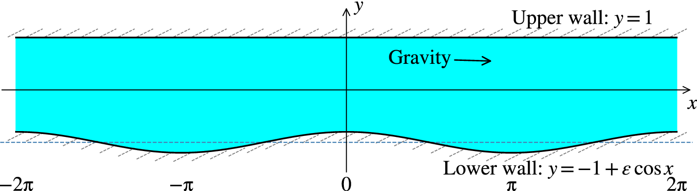
We consider incompressible steady Stokes flow of a viscous fluid in two dimensions, with gravitational body force along the channel. The problem is described by the continuity equation, and the Navier–Stokes equation with the convective terms removed. The system is nondimensionalised using the channel half-height H and other scalings as given in our recent paper [Reference Walters and Forbes15]. The upper wall is a flat surface located at $y=1$ , but the lower wall has a sinusoidal shape $f(x)$ with dimensionless period $2\pi $ and amplitude $\epsilon $ , and is centred at $y = -1$ . In this paper we choose $f(x)=~\cos x$ . A sketch of the dimensionless channel configuration is given in Figure 1. For convenience, we choose the channel to have aspect ratio $\pi $ (wall wavelength over channel width), but generalisation to different ratios is straightforward, and is pursued at the end of Section 4.

Figure 1

A schematic of the 2D channel with $-1+\epsilon \cos x<y<1$ and $\pi $ -periodic in x. Gravity points along the channel in the $+x$ direction.

In 2D flow, there are two velocity components u and v, and P denotes pressure. Conservation of mass requires

$$ \begin{align*} u_x + v_y = 0, \end{align*} $$

and the two components of the linearised Navier–Stokes equation, appropriate for slow Stokes flow of a viscous fluid, are

(2.1) $$ \begin{align} u_{xx} + u_{yy} & = P_x - 2 , \end{align} $$

(2.2) $$ \begin{align}v_{xx} + v_{yy} & = P_y. \end{align} $$

The viscous no-slip boundary condition on the upper wall in Figure 1 is simply

$$ \begin{align*} u=0 , v=0 \quad\textrm{on } y=1, \end{align*} $$

and on the lower wall

$$ \begin{align*} u=0 , v=0 \quad\textrm{on } y = -1 + \epsilon \cos x. \end{align*} $$

Notice that the gravitational body force along the channel is chosen to be $2$ in our nondimensionalisation, to give the simple form (2.5) for the Poiseuille profile. This body force term is also equivalent to an applied mean pressure gradient $dP/dx=-2$ .

This system is now subjected to a perturbation expansion in the small parameter $\epsilon $ , which is the amplitude of the lower wall function:

(2.3) $$ \begin{align}\begin{aligned} u&=u_0+\epsilon u_1+\epsilon^2 u_2+\cdots,\\ v&=v_0+\epsilon v_1+\epsilon^2 v_2+\cdots,\\ P&=P_0+\epsilon P_1+\epsilon^2 P_2+\cdots. \end{aligned} \end{align} $$

The lower boundary conditions also must be expanded in terms of $\epsilon $ :

(2.4) $$ \begin{align}\begin{aligned} & u(x,-1+\epsilon \cos x)=0, \\ & u_0(x,-1)+\epsilon u_1(x,-1) +\epsilon \cos x \frac{\partial u_0}{\partial y}(x,-1)+\cdots=0, \end{aligned}\end{align} $$

and similarly for v. The upper boundary conditions are simply $0=u_n=v_n$ on $y=1$ at every order n.

Applying the zeroth-order boundary conditions, $u=v=0$ on $y=-1$ , the zeroth-order solution is straightforward, yielding the parabolic profile flow

(2.5) $$ \begin{align}\begin{aligned} u_0&=1-y^2,\\ v_0&=0,\\ P_0&=0. \end{aligned}\end{align} $$

Matching terms at $\mathcal {O}(\epsilon )$ , the first-order system is

$$ \begin{align*} u_{1,x}+v_{1,y}&=0,\\ u_{1,xx}+u_{1,yy}&=P_{1,x},\\ v_{1,xx}+v_{1,yy}&=P_{1,y}, \end{align*} $$

with lower boundary conditions from (2.4):

(2.6) $$ \begin{align}\begin{aligned} u_1(x,-1)&=-2\cos x,\\ v_1(x,-1)&=0. \end{aligned}\end{align} $$

The continuity equation may be satisfied in the usual way, by defining velocity components at each order in terms of a stream function $\psi $ , such that

$$ \begin{align*} u_n=\frac{\partial \psi_n}{\partial y},\quad v_n=-\frac{\partial \psi_n}{\partial x}. \end{align*} $$

Then, subtracting the x-derivative of (2.2) from the y-derivative of (2.1), we arrive at the biharmonic equation

$$ \begin{align*} \frac{\partial^4 \psi_n}{\partial x^4}+2\frac{\partial^4 \psi_n}{\partial x^2 \partial y^2}+\frac{\partial^4 \psi_n}{\partial y^4}&=0, \end{align*} $$

subject to $u_n=v_n=0$ on $y=1$ (these top wall boundary conditions are zero for every mode m at each order n),with $u_n$ and $v_n$ specified on $y=-1$ . At each order n, we isolate each mode m such that $u_n=\sum _m U_{n,m}$ , $v_n=\sum _m V_{n,m}$ , and we write the solution as

$$ \begin{align*} U_{n,m}&=\cos(mx)F_{n,m}(y),\\ V_{n,m}&=\sin(mx)G_{n,m}(y), \end{align*} $$

where $G_{n,m}'=m F_{n,m}$ to satisfy continuity. That is, $\psi _{n,m}=\cos (mx) G_{n,m}(y)/m$ , $m>0$ . Incorporating the top wall boundary conditions, we may write a general solution for $F_{n,m}$ and $G_{n,m}$ in the forms

(2.7) $$ \begin{align}\begin{aligned} F_{n,m}&=(m A_{n,m} (1-y) \cosh[m(1-y)]\\ &\quad+(A_{n,m}+B_{n,m}(1-y)) \sinh[m(1-y)] )/\cosh(2m),\\ G_{n,m}&=(-B_{n,m}(1-y) \cosh[m(1-y)]\\ &\quad+(B_{n,m}/m-m A_{n,m}(1-y)) \sinh[m(1-y)] )/\cosh(2m), \end{aligned} \end{align} $$

where the constants $A_{n,m}$ and $B_{n,m}$ are determined from the boundary conditions for $U_{n,m},V_{n,m}$ on $y=-1$ . The constant denominator term is included to improve numerical stability.

To illustrate the procedure, we first solve for $u_1$ . On $y=-1$ , we have $u_1=-2\cos (x)$ , as in (2.6). We therefore look for a solution $u_1(x,y)=\cos (x) F_1(y)$ , leading to

$$ \begin{align*} F_1^{IV}-2F_1^{II}+F_1=0. \end{align*} $$

Using the general solution and applying the lower boundary conditions (2.6), we find

(2.8) $$ \begin{align}\begin{aligned} A_{1,1}&= \frac{\sinh (4)-4 \cosh^2 (2)}{4-\sinh ^2(2)},\\ B_{1,1}&=\frac{2\sinh (4)}{4-\sinh ^2(2)}. \end{aligned} \end{align} $$

These constants define $u_1$ and $v_1$ , noting that only the single mode $m=1$ is nonzero.

Now the bulk flux through the channel may be calculated at any x, by integrating u from bottom to top. The bulk flux should be independent of x. This provides a useful check for the algorithm, where we can examine the flux at each cosine mode, to confirm that for $m>0$ , the flux at that mode is zero:

(2.9) $$ \begin{align} Q=\int_{y=f(x)}^{y=1} u\, dy. \end{align} $$

Suppose that $q(y)=\int u \,dy$ is an antiderivative of the velocity component u. Then

(2.10) $$ \begin{align} Q&=q(1)-q(-1+\epsilon \cos(x))\nonumber\\ &=\int^1_{-1} u_0 \,dy + \epsilon \int^1_{-1} u_1 \,dy - \epsilon \cos(x) u_0(x,-1)+\mathcal{O}(\epsilon^2). \end{align} $$

Therefore at zeroth order, the contribution to the flux in (2.9) is

$$ \begin{align*} Q_0&=\int_{-1}^1 u_0\, dy = 4/3. \end{align*} $$

At first order, the $\epsilon ^1$ terms in (2.10) evaluate to zero, so the first-order contribution to the flux is zero ( $Q_1=0$ ).

Employing the coefficients $A_{1,1},B_{1,1}$ from (2.8) in the general form (2.7), the velocity components at first order are

$$ \begin{align*} u_1&=\cos x [A_{1,1} (1-y) \cosh(1-y)+(A_{1,1}+B_{1,1}(1-y)) \sinh(1-y) ]/\cosh(2), \\ v_1&=\sin x [-B_{1,1} (1-y) \cosh(1-y)+(B_{1,1}-A_{1,1}(1-y)) \sinh(1-y) ]/\cosh(2). \end{align*} $$

By taking the y-derivative (signified using prime notation), and setting $y=-1$ , on simplification we obtain derivatives on the lower boundary (for the next order calculations)

$$ \begin{align*} u_1'|_{-1}&=\frac{4 (-1-8 e^4+e^8) \cos (x)}{1-18 e^4+e^8}, \\ v_1'|_{-1}&=2 \sin (x). \end{align*} $$

At second order, the boundary conditions on $y=-1$ are

$$ \begin{align*} u_2&=- f u_1'-\frac{f^2}{2}u_0"\\ &=- \cos^2(x) \, \bigg(\frac{4 (-1-8 e^4+e^8)}{1-18 e^4+e^8}-1\bigg)\,,\\ v_2&=-f v_1'=-2\sin(x)\cos(x)=-\sin(2x), \end{align*} $$

where $f(x)=\cos (x)$ is the lower boundary function. Since the boundary condition for $u_2$ involves the function $\cos ^2(x) = \tfrac 12+\tfrac 12 \cos (2x)$ , $u_2$ is expected to involve both a zeroth- and a second-order mode in x. Therefore we make the ansatz

$$ \begin{align*} u_2&=U_{2,0}+U_{2,2} \cos(2x),\\ v_2&= V_{2,2} \sin(2x). \end{align*} $$

Look at the mean component $U_{2,0}$ . The steady Stokes equations give

$$ \begin{align*} \partial_{yy}U_{2,0}= \partial_x P_{2,0}=0, \end{align*} $$

so the zero mode is a linear function: $U_{2,0}=A_{2,0}+B_{2,0} y$ . The upper boundary condition requires $A_{2,0}=-B_{2,0}$ , allowing us to write $U_{2,0}=A_{2,0}(1-y)$ . The lower boundary condition sets the value of this single constant $A_{2,0}$ , so that

$$ \begin{align*} U_{2,0}&= (1-y)\bigg(\frac{1+8 e^4-e^8}{1-18 e^4+e^8}+\frac{1}{4}\bigg)\,. \end{align*} $$

The mean flux term for this component is then

$$ \begin{align*} Q_{2,0}= \int_{-1}^1 (1-y)A_{2,0} \, dy = 2A_{2,0} =2\,\bigg(\frac{1+8 e^4-e^8}{1-18 e^4+e^8}+\frac{1}{4}\bigg)\,, \end{align*} $$

and total flux at second order is

$$ \begin{align*} Q_{2}&= \int_{-1}^1 U_{2,0} \, dy - \cos(x) u_1(-1)-\frac12 \cos^2(x) u^{\prime}_0(-1) = 2\frac{1+8 e^4-e^8}{1-18 e^4+e^8}+1. \end{align*} $$

We may now solve for the mode-2 components, using the same form:

$$ \begin{align*} F_{2,2}&=(2 A_{2,2} (1-y) \cosh[2(1-y)]+(A_{2,2}+B_{2,2}(1-y)) \sinh[2(1-y)] )/\cosh(4),\\ G_{2,2}&=(-B_{2,2}(1-y) \cosh[2(1-y)]+(B_{2,2}/2-2 A_{2,2}(1-y)) \sinh[2(1-y)] )/\cosh(4). \end{align*} $$

Applying boundary conditions gives the two equations for $A_{2,2}$ and $B_{2,2}$ .

This procedure may be automated. In general, the boundary conditions at order n are

(2.11) $$ \begin{align} u_n=-\sum_{m=1}^n \frac{f^m}{m!} \partial_y^m u_{n-m}. \end{align} $$

The flux is expanded as $Q=\sum _{n=0}^N \epsilon ^n Q_n$ and

(2.12) $$ \begin{align} Q_n = \int_{-1}^{1} u_n \, dy - \sum_{k=1}^{n} \frac{f^k}{k!} \partial_y^{k-1} u_{n-k}\bigg|_{y=-1}. \end{align} $$

We automated this task in Mathematica. This yielded large symbolic expressions for the flux, which was computable in a reasonable time up to order $\mathcal {O}(\epsilon ^{10})$ , but which required a long time to compute for order $\mathcal {O}(\epsilon ^{12})$ , and more so for $\mathcal {O}(\epsilon ^{14})$ . The same task was then automated to give numerical solutions in Fortran. With careful numerics, this returns the bulk flux up to $\mathcal {O}(\epsilon ^N)$ , where at $N=160$ the numerics still appear stable. After that point, the high-order derivatives introduce very large coefficient values that are difficult to control accurately, although we expect that further refinements would allow increase in N.

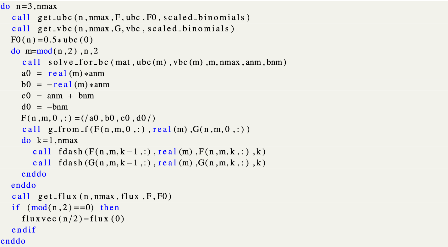
For clarity, we present the main loop for this algorithm for $n>2$ in Figure 2. First the boundary conditions are found for $u_n$ and $v_n$ , in terms of the modes up to n. The single coefficient for the mode-0 part of u is just $A_{n,0}=U^{BC}_0/2$ . Then the two coefficients $A_{n,m}, B_{n,m}$ are found for each mode, using the boundary conditions for that mode, and mat is the $2 \times 2$ matrix:

$$ \begin{align*} \textrm{mat}(m) = \bigg(\begin{matrix} 2 m+\tanh(2m) & 2 \tanh(2m) \\ -2 m \tanh(2m) & -2+\tanh(2m)/m \end{matrix}\bigg)\,. \end{align*} $$

Figure 2

The central loop of the algorithm for finding the coefficients for the $\epsilon $ expansion.

Figure 2 Long description

The code begins with an outer loop: do n equals 3, n max. Inside this loop, two functions are called: get underscore u b c and get underscore v b c, both taking arguments n, n max, F or G, u b c or v b c, F 0, and scaled underscore binomials. F 0 of n is then set to 0.5 times u b c of 0.

A nested loop follows: do m equals mod of n, 2, n, 2. Inside this loop:

- A call to solve underscore for underscore b c with arguments mat, u b c of m, v b c of m, m, n max, a n m, and b n m.

- Variable assignments: a 0 equals real of m times a n m; b 0 equals minus real of m times a n m; c 0 equals a n m plus b n m; d 0 equals minus b n m.

- F of n, m, 0, colon is assigned the array a 0, b 0, c 0, d 0.

- A call to g underscore from underscore f.

- A third nested loop: do k equals 1, n max, which calls f dash twice for F and G arrays using k minus 1 and k indices.

- The m loop ends with enddo.

After the m loop, a call to get underscore flux is made. An if statement checks if mod of n, 2 equals 0; if true, fluxvec of n over 2 is assigned flux of 0. The outer n loop concludes with enddo.

Four new constants $a,b,c,d$ are formed from the two coefficients $A_{n,m}, B_{n,m}$ such that $F=(a + b y)\cosh (m(1-y))+(c+d y)\sinh (m(1-y))$ . This allows differentiation and integration of F and G any number of times, as simple linear transformations of $a,b,c,d$ . These coefficients are stored for F, G and their derivatives. In fact, these derivatives involve coefficients that are multiplied by m for each succeeding derivative, which is numerically problematic. In the boundary condition calculations, however, the derivatives are divided by $m!$ , so the derivative coefficients are calculated and stored with this factor. This change greatly increased the numerical stability of the program. These coefficients are then used to calculate the flux at each order n.

The helper routines in Figure 2 are as follows. The call to get_ubc implements equation (2.11), assembling the u boundary condition at each Fourier mode by summing contributions from all lower-order solutions. The call to get_vbc does the same for v. Boundary conditions are solved using solve_for_bc, which solves the $2 \times 2$ system $\text {Mat}(m)(A_{n,m},B_{n,m})^T = (U^{bc}_{n,m},V^{bc}_{n,m})^T$ to find the two free constants in $U_{n,m}$ that satisfy the boundary condition at $y=-1$ . The $V_{n,m}$ coefficients are derived from the $U_{n,m}$ coefficients in g_from_f via the incompressibility constraint. All derivatives of F and G are computed in coefficient space using the fdash routine up to the highest order required. Finally, the flux is calculated using get_flux, which implements equation (2.12).

With $f = \cos x$ , the boundary condition (2.11) may be projected onto each Fourier mode m by expanding $f^k \cos (m'x)$ as a sum of $\cos (mx)$ terms. Using the identity

$$ \begin{align*} \cos^k(x) = 2^{-(k+1)}\sum_{j=0}^{k} \binom{k}{j}\cos((k-2j)x), \end{align*} $$

we have

$$ \begin{align*} \cos^k(x)\cos(m'x) = \sum_{m=0}^{\infty} C(k,m',m)\cos(mx), \end{align*} $$

where the coefficients $C(k,m',m)$ are obtained by collecting terms with the same argument. The boundary condition for each Fourier mode m of $u_n$ then becomes

$$ \begin{align*} U^{bc}_{n,m} = -\sum_{k=1}^{n-1}\sum_{m'=1}^{n-k} \frac{1}{k!}\partial_y^k U_{n-k,m'}\bigg|_{y=-1} C(k,m',m), \end{align*} $$

and analogously for $V^{bc}_{n,m}$ , with $\cos (m'x)$ replaced by $\sin (m'x)$ in the product with $f^k$ . scaled_binomials stores the precomputed coefficients for this sum. It holds the required values $S(m,j)=2^{-(m+1)}\binom {m}{j}$ .

Finally, we note that the parity constraint on the modes do m=mod(n,2),n,2, that is, at order n only modes of the same parity contribute, is a consequence of $f=\cos (x)$ containing a single Fourier mode. This constraint simplifies the computation in our case, but would not be appropriate for a more general boundary. The Fortran code is available on reasonable request to the first author.

All calculations are performed in coefficient space, making the routine very fast. For comparison, on a single-thread on an i7-7700K CPU, with $N\max =180$ , the program took less than a second at double precision, which gave numerically sensible results out to $\mathcal {O}(\epsilon ^{60})$ . At quad precision, the program took just under $10$ seconds, and gave numerically sensible results out to $\mathcal {O}(\epsilon ^{160})$ .

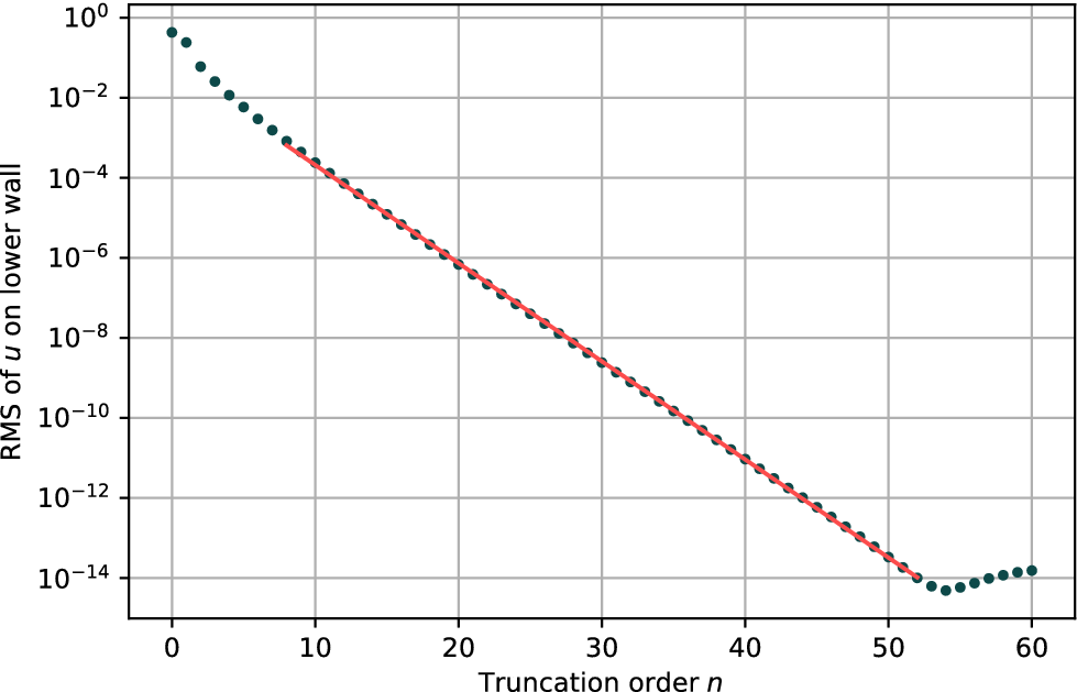
The convergence of the series is demonstrated in Figure 3, which shows the average root-mean-square (RMS) value of u on the boundary for the series solution truncated at order n. In this case, we chose $\epsilon =0.3$ , and used double-precision reals. The residual decays exponentially with truncation order, as expected for a convergent power series. After the initial points, a least-squares fit to our results showed that the error behaves as $RMS_{\text {error}}\approx \exp (-0.565 n)$ , and this is drawn using a red line in Figure 3.

Figure 3

The average RMS of the velocity component u on the lower wall as a function of order n, shown with blue dots. The lower boundary parameter was fixed at $\epsilon =0.3$ . The series shows exponential convergence down to the double-precision floor near $n=53$ , beyond which a small amount of floating-point noise accumulates. A linear fit to the central data points is shown as a red line, suggesting that the RMS error decays as $\exp (-0.565 n)$ .

Figure 3 Long description

The horizontal x-axis is labeled Truncation order n with a linear scale from 0 to 60. The vertical y-axis is labeled R M S of u on lower wall with a logarithmic scale ranging from 10 super 0 down to 10 super minus 14.

* From n equals 0 to 8, blue dots show a rapid initial decrease in R M S values from nearly 10 super 0 to 10 super minus 3.

* From n equals 8 to 53, the data points follow a strict downward linear trend on this semi-log plot. A solid red line is overlaid on these points, indicating a constant rate of exponential convergence.

* At n equals 53, the R M S reaches its minimum value near 10 super minus 14, which is the double-precision floor.

* Beyond n equals 53, the blue dots show a slight upward trend with scattered positioning, representing the accumulation of floating-point noise.

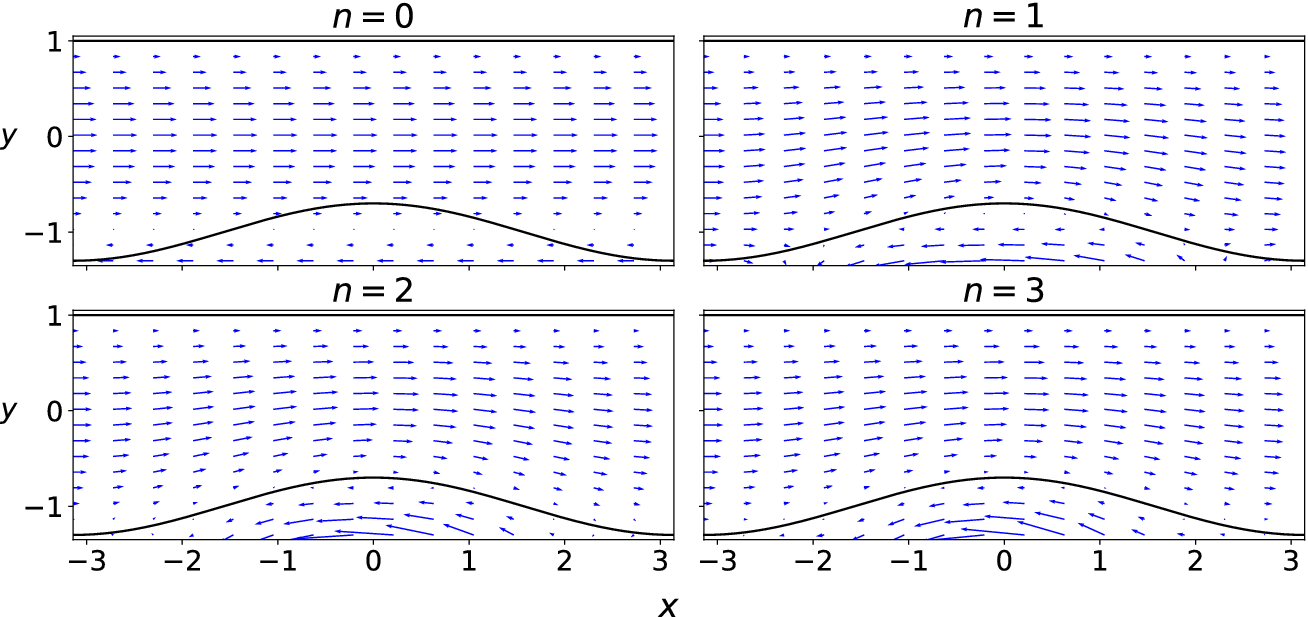
A quiver plot is shown in Figure 4, showing this convergence at the lowest orders. At $n=0$ , the flow is pure Poiseuille, passing straight through the lower wall. As each higher-order term is added, the flow is progressively adjusted in the channel and in the nonphysical region below the wall to enforce the no-slip condition.

Figure 4

Quiver plots of the velocity field for the series truncated at orders $n=0,1,2,3$ , showing the adjustment of the flow to correctly match the no-slip condition on the wavy wall. The lower boundary parameter was again fixed at $\epsilon =0.3$ . The flow field for $n>3$ is visually identical to the $n=3$ plot.

Figure 4 Long description

A four-panel grid of quiver plots. Each panel shares a horizontal x-axis ranging from negative 3 to 3 and a vertical y-axis ranging from negative 1 to 1. A flat boundary exists at y equals 1, and a sinusoidal wavy wall is centered at the bottom. Blue arrows represent velocity vectors.

* Top-left panel (n = 0): The velocity vectors are strictly horizontal and uniform across the channel. The arrows penetrate the wavy wall boundary, indicating the no-slip condition is not yet met.

* Top-right panel (n = 1): The vectors begin to tilt and follow the contour of the wavy wall. Small recirculating or counter-flow arrows appear in the trough regions below the wall peak.

* Bottom-left panel (n = 2): The flow field shows increased adjustment. The vectors above the wavy wall curve more distinctly to match the boundary shape, and the vectors below the wall peak are more pronounced in their opposite direction.

* Bottom-right panel (n = 3): The velocity field is now fully adjusted. The vectors perfectly tangent the wavy wall surface, and a clear secondary flow pattern is visible in the region below the peak, satisfying the no-slip condition on the complex boundary.

3 Numerical solution of the Stokes equations

We seek an accurate numerical solution for the steady Stokes equations to compare with the very high-order expansions of the previous section. We start by using spectral basis functions that meet the boundary conditions precisely. This is the no-slip-Chebyshev (NSC) basis described by the current authors [Reference Walters and Forbes15]. Also, we incorporate the conformally mapped equations described there, but with the nonlinear (inertial) terms removed. The steady Stokes equations are numerically stiff, but linear, so we choose to solve the large matrix equations using the generalised minimal residual (GMRES) method [Reference Saad9], to avoid storing and manipulating very large matrices.

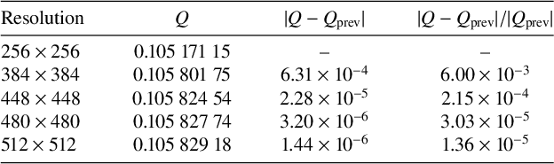
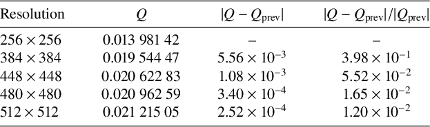
In summary, the numerical method uses a periodic Fourier basis in x and an NSC basis in y, a stream function to assert incompressibility, and a numerical conformal mapping to map the system to a rectangular computational region. A GMRES method is used with the residual forced below $10^{-10}$ , ensuring that the linear system was solved to high accuracy at each grid resolution. Grid convergence was then assessed by comparing the bulk flux Q across successive refinements (Tables 1 and 2). For $\epsilon <1.5$ , convergence is rapid, agreeing with the results from coarser grids to at least four significant figures. For higher values of $\epsilon $ , the results are converged to at least one significant figure with a $512\times 512$ grid. For maximum $\epsilon =1.95$ , approaching the pinch-off limit $\epsilon \to 2$ , the numerical solver struggles at lower grid resolutions, but comparing the $512\times 512$ results with a longer run on a $768\times 768$ grid, we found that the results agreed with the $512\times 512$ results to two significant figures, $Q = 2.7 \times 10^{-4}$ on both 512 and 768 grids. We consider this level of accuracy sufficient for comparison with the series expansion.

Table 1

Grid convergence of bulk flux Q at $\epsilon = 1.50$ . Each row shows the change relative to the previous refinement level.

Table 1 Long description

The table consists of four columns: Resolution, Q, absolute difference between Q and Q sub prev, and relative difference between Q and Q sub prev.

* Row 1: Resolution 256 times 256; Q is 0.105 171 15; differences are not applicable.

* Row 2: Resolution 384 times 384; Q is 0.105 801 75; absolute difference is 6.31 times 10 super minus 4; relative difference is 6.00 times 10 super minus 3.

* Row 3: Resolution 448 times 448; Q is 0.105 824 54; absolute difference is 2.28 times 10 super minus 5; relative difference is 2.15 times 10 super minus 4.

* Row 4: Resolution 480 times 480; Q is 0.105 827 74; absolute difference is 3.20 times 10 super minus 6; relative difference is 3.03 times 10 super minus 5.

* Row 5: Resolution 512 times 512; Q is 0.105 829 18; absolute difference is 1.44 times 10 super minus 6; relative difference is 1.36 times 10 super minus 5.

Table 2

Grid convergence of bulk flux Q at $\epsilon = 1.75$ . Higher grid refinement is needed for convergence of results in this very constricted channel.

Table 2 Long description

The table consists of four columns and five data rows.

Column headers are:

1. Resolution.

2. Q.

3. Absolute value of Q minus Q sub prev.

4. Absolute value of Q minus Q sub prev all over Q sub prev.

Data rows:

* Resolution 256 times 256: Q is 0.013 981 42. Differences are not applicable.

* Resolution 384 times 384: Q is 0.019 544 47. Absolute difference is 5.56 times 10 super minus 3. Relative difference is 3.98 times 10 super minus 1.

* Resolution 448 times 448: Q is 0.020 622 83. Absolute difference is 1.08 times 10 super minus 3. Relative difference is 5.52 times 10 super minus 2.

* Resolution 480 times 480: Q is 0.020 962 59. Absolute difference is 3.40 times 10 super minus 4. Relative difference is 1.65 times 10 super minus 2.

* Resolution 512 times 512: Q is 0.021 215 05. Absolute difference is 2.52 times 10 super minus 4. Relative difference is 1.20 times 10 super minus 2.

First the numerical conformal mapping was performed for $\epsilon =0$ to $\epsilon =1.95$ in steps of $0.05$ . The mapped lower wall location was compared with the analytic function $y=~\!\!\!-1+\epsilon \cos x$ , and the grid refined until agreement was satisfactory. For the mapping code, a $3200 \times 3200$ grid was used, generating 2400 mapping coefficients. At this resolution, the absolute maximum difference was near machine precision ( $10^{-12}$ ) up to $\epsilon =1.6$ , dropping to $8\times 10^{-4}$ for $\epsilon =1.95$ . For each value of $\epsilon $ , the 2400 coefficients that determine the mapping were stored to disk to be used by the GMRES Stokes solver. For the 40 values of $\epsilon $ these mappings took 420 minutes to complete (roughly $10$ minutes each).

4 Comparison of results

The purely numerical results (stars) are compared with the results of the perturbation expansion at various orders (dashed-dotted lines) in Figure 5. At the lowest approximation, $\mathcal {O}(\epsilon ^2)$ , the perturbation expansion agrees with the numerical data up to $\epsilon \approx 0.25$ . The higher-order terms improve this agreement up to $\epsilon =0.9$ . However, near $\epsilon =0.95$ , the series appears to diverge for all orders, the highest shown being $\mathcal {O}(\epsilon ^{180})$ . Therefore, diagonal Padé approximants were formed from the coefficients in order to model the flux beyond that point. These approximants are shown with solid lines. It may be seen that all the Padé approximants higher than the [3/3] visually match the numerical results.

Figure 5

The bulk flux at various amplitudes of the lower wall function, from straight channel ( $\epsilon =0$ ) to the point where the lower wall amplitude is just large enough to pinch off the opening ( $\epsilon =2$ ). The stars are the numerical results, for $\epsilon =0, 0.05, 0.1, \cdots , 1.95$ . The dashed-dotted lines are the results of the perturbation expansion, diverging near $\epsilon =0.95$ , with the highest-order results being the steepest at that point. The solid lines are the first six diagonal Padé approximants, based on the perturbation coefficients. The [4/4] to [6/6] approximants are visually indistinguishable.

Figure 5 Long description

The X axis represents Wall Amplitude epsilon from 0.00 to 2.00. The Y axis represents Bulk Flux Q from negative 0.2 to 1.4.

* Numerical results are shown as blue stars, starting at Q equals 1.33 when epsilon is 0 and decreasing smoothly to 0 as epsilon approaches 2.0.

* Perturbation expansion results are shown as dashed-dotted lines. These follow the numerical data until approximately epsilon equals 0.75, where they begin to diverge wildly. Near epsilon equals 0.95, these lines shoot vertically toward positive and negative infinity.

* Padé approximants are shown as solid colored lines.

* Padé 1/1 (blue) and 2/2 (orange) deviate from the numerical stars after epsilon equals 1.0.

* Padé 3/3 (green) shows a large upward curve after epsilon equals 1.5.

* Padé 4/4 (red), 5/5 (purple), and 6/6 (brown) are visually indistinguishable from each other and closely track the numerical stars across the entire range from 0 to 2.0.

* A horizontal dashed black line marks the Q equals 0 baseline.

Padé approximants $[m/n]$ are rational functions involving the first $m+n+1$ coefficients of a power series, whose Maclaurin expansion agrees with the original power series to order $m+n$ . Full details may be found in Baker and Graves-Morris [Reference Baker and Graves-Morris2]. The lowest-order Padé approximant uses the three lowest coefficients from the series $c_0, c_1, c_2$ in the form

$$ \begin{align*} c_0&=4/3,\\ c_1&=-\frac{-3+2 e^4+e^8}{1-18 e^4+e^8}\approx -1.544\,201\,551\,917\,25, \\ c_2&=\frac{n_{11}}{d_{11}}\approx 1.265\,778\,229\,812\,035,\\ n_{11}&=-45+1012 e^4+15\,572 e^8+26\,284 e^{12}-4566 e^{16}\\ &\quad -1652 e^{20}-3804 e^{24}-44 e^{28}+11 e^{32},\\ d_{11}&=16 (1-18 e^4+e^8)^2 (1-66 e^8+e^{16}),\\ Q_{11}&=\frac{c_0 c_1+(c_1^2-c_0c_2)\epsilon^2}{c_1-c_2\epsilon^2}\approx \frac{2.058\,935\,4-0.696\,854 \epsilon^2}{1.544\,202+1.265\,778 \epsilon^2}. \end{align*} $$

Even this simple ratio is surprisingly accurate, visually matching the numerical results up to about $\epsilon =0.75$ . At higher orders, the form of the exact coefficients quickly becomes unwieldy, but they can always be approximated by their numerical values to 16 significant figures as

(4.1) $$ \begin{align}\begin{aligned} c_3&\approx-1.145\,261\,858\,484\,969, \\ c_4&\approx1.114\,570\,034\,610\,418. \end{aligned}\end{align} $$

The [2/2] approximant uses the first five coefficients ( $c_0,c_1,c_2,c_3,c_4$ ) in the form

(4.2) $$ \begin{align}\begin{aligned} n_{22}&=c_0 (c_2^2-c_1 c_3)+(c_1(c_2^2-c_1c_3)+c_0(c_1c_4-c_2c_3))\epsilon^2 \\ &\quad+(c_0(c_3^2-c_2c_4)+c_1(c_1c_4-c_2c_3)+c_2(c_2^2-c_1c_3))\epsilon^4 ,\\ d_{22}&=c_2^2-c_1c_3+(c_1c_4-c_2c_3)\epsilon^2+(c_3^2-c_2c_4)\epsilon^4,\\ Q_{22}&=\frac{n_{22}}{d_{22}}\approx \frac{0.221\,761+0.105\,132\epsilon^2-0.076\,452\,7\epsilon^4}{0.166\,321+0.271\,473\epsilon^2+0.099\,173\,8 \epsilon^4}. \end{aligned} \end{align} $$

From Figure 5, we see that this is visually accurate up to about $\epsilon =1.1$ . Each Padé approximant is found by solving a small linear system involving the coefficients. By the time we have the [4/4] approximant, the results visually match the numerical results. Higher-order Padé approximants ( $n> 4$ ) agree very closely with the lower-order approximants and numerical results, with the higher-order approximants giving some small gains near $\epsilon =2$ , where the flux should be zero (the channel is pinched shut at $\epsilon =2$ ). These Padé approximants ameliorate the divergence of the series at $\epsilon =0.95$ , and are a very effective way to accurately approximate the bulk flux with very little computation time.

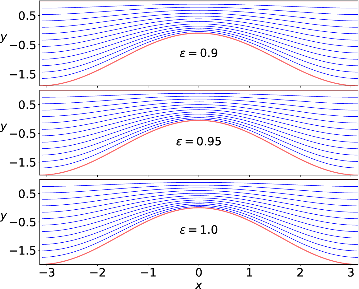
There is no obvious physical reason why the series diverges near $\epsilon =0.95$ . In Figure 6, the streamlines are plotted from the numerical data for wall amplitude $\epsilon =0.9,0.95,1$ . Apart from the small change in the wall shape, the flow may be seen to remain largely the same in each panel, showing no recirculation zones or topological changes across the divergence threshold, indicating that there is no obvious physical mechanism for the divergence of the perturbation expansion near $\epsilon =0.95$ .

Figure 6

Streamlines for values of $\epsilon $ near 0.95, where the perturbation series diverges. The flow appears largely unchanged, indicating that the divergence is not related to any physical mechanism.

Figure 6 Long description

The figure consists of three vertically stacked panels, each sharing an x-axis ranging from minus 3 to 3 and a y-axis ranging from minus 1.5 to 0.5.

* The top panel is labeled epsilon equals 0.9. It shows a thick red curve at the bottom representing a hump centered at x equals 0. Above this red curve, approximately 15 blue streamlines follow the contour of the hump, becoming flatter as they move higher in the y-direction.

* The middle panel is labeled epsilon equals 0.95. The visual structure is nearly identical to the top panel, with blue streamlines maintaining a smooth, laminar flow over the central red hump.

* The bottom panel is labeled epsilon equals 1.0. The streamlines and the red boundary curve remain consistent with the previous two panels, showing no signs of turbulence or structural change despite the increasing epsilon value.

In all three panels, the streamlines are densest near the peak of the hump at x equals 0 and spread out as they move toward the lateral boundaries at x equals minus 3 and x equals 3.

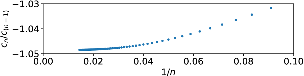
To investigate this further, we present a Domb–Sykes plot [Reference Domb and Sykes4] in Figure 7. This shows the ratio of the coefficients $c_n/c_{n-1}$ plotted against $1/n$ . The rationale for this is that for a series $\sum c_n \epsilon ^{2n}$ , the ratio $c_n/c_{n-1}$ converges to $1/\epsilon ^2_c$ , where $\epsilon ^2_c$ is the radius of convergence. The first ten points have been excluded while the series settles down, leaving the ratios for coefficients of $\epsilon ^{20}$ to $\epsilon ^{160}$ . It is apparent that the ratios are still not in the linear regime, but it may be seen that the curve will cross the axis somewhere near $-1.0485$ . This suggests a singularity near $\epsilon ^2 \approx -1/1.0485 \approx -0.95$ . This shows good agreement with the divergence of the series, seen in Figure 5 near $\epsilon \approx \sqrt {0.95}\approx ~0.97$ .

Figure 7

A Domb–Sykes plot of the ratios of the coefficients of the power series in $\epsilon ^2$ against $1/n$ . The ratios are converging near $-1.0485$ .

Van Dyke [Reference Van Dyke14] and Domb and Sykes [Reference Domb and Sykes4] argue further that both the intercept and slope of the Domb–Sykes plot yield information about the radius of convergence and the nature of the nearest singularity. In order to study these further, we next applied Aitken’s $\Delta ^2$ extrapolation method [Reference Aitken1] on the ratio data in an attempt to clarify the intercept and slope of the Domb–Sykes plot. We define the sequence of ratios $S_n=c_n/c_{(n-1)}$ and seek to estimate its limit as $n\rightarrow \infty $ . To estimate this limit, the Aitken transform computes a new sequence as

$$ \begin{align*} S^E_n&=\frac{S_{n+1}S_{n-1}-S_n^2}{S_{n+1}-2S_n+S_{n-1}}. \end{align*} $$

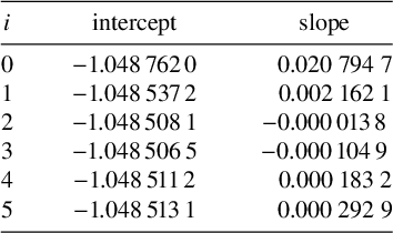
The extrapolated terms $S^E_n$ form a new sequence with two fewer terms. This procedure may be repeated with the new sequence $S^E$ . Five such extrapolations were performed and a linear fit applied to the last ten points to give an estimate of the intercept and slope at each level. The results are shown in Table 3 both for the original coefficient ratios, and also after extrapolation up to five times. The intercept appears to stabilise after only two extrapolations.

Table 3

Intercept and slope for the coefficient ratio data. The first column i indicates the number of repeated Aitken extrapolations used. The intercept appears stable after two extrapolations.

Table 3 Long description

The table consists of three columns labeled i, intercept, and slope.

* Row 1: i is 0, intercept is -1.048, 762, 0, slope is 0.020 794 7.

* Row 2: i is 1, intercept is -1.048, 537, 2, slope is 0.002 162 1.

* Row 3: i is 2, intercept is -1.048, 508, 1, slope is 0.000, 013, 8.

* Row 4: i is 3, intercept is -1.048, 506, 5, slope is -0.000, 104, 9.

* Row 5: i is 4, intercept is -1.048, 511, 2, slope is 0.000 183 2.

* Row 6: i is 5, intercept is -1.048, 513, 1, slope is 0.000 292 9.

For a singularity of the form $(\epsilon ^2+\epsilon _c^2)^\alpha $ , the coefficient ratio has the form $c_n/c_{n-1}\sim (1/\epsilon _c^2)(1-(1+\alpha )/n) $ so that the Domb–Sykes plot has a slope proportional to $\alpha +1$ . The zero slope suggested by the data in Table 3 would imply $\alpha =-1$ : a simple pole. This pole is located approximately at $\epsilon ^2=-1/1.048\,51=-0.953\,73$ , closely matching the visual estimate of the intercept and a zero in each of the Padé denominators. This also agrees well with the apparent radius of convergence limitation apparent in Figure 5. In terms of $\epsilon $ the singularity is therefore on the imaginary axis at $\pm \sqrt {0.954} i\approx \pm 0.977i$ . This suggests that the divergence of the series is not connected to any geometric feature of the physical channel, but reflects the analytic structure in the complex $\epsilon $ plane. Mathematically, therefore, the series (2.3) close to the nearest singularity behaves as $(\epsilon -0.977i)^{-1}(\epsilon +0.977i)^{-1}=(\epsilon ^2+0.954)^{-1}$ .

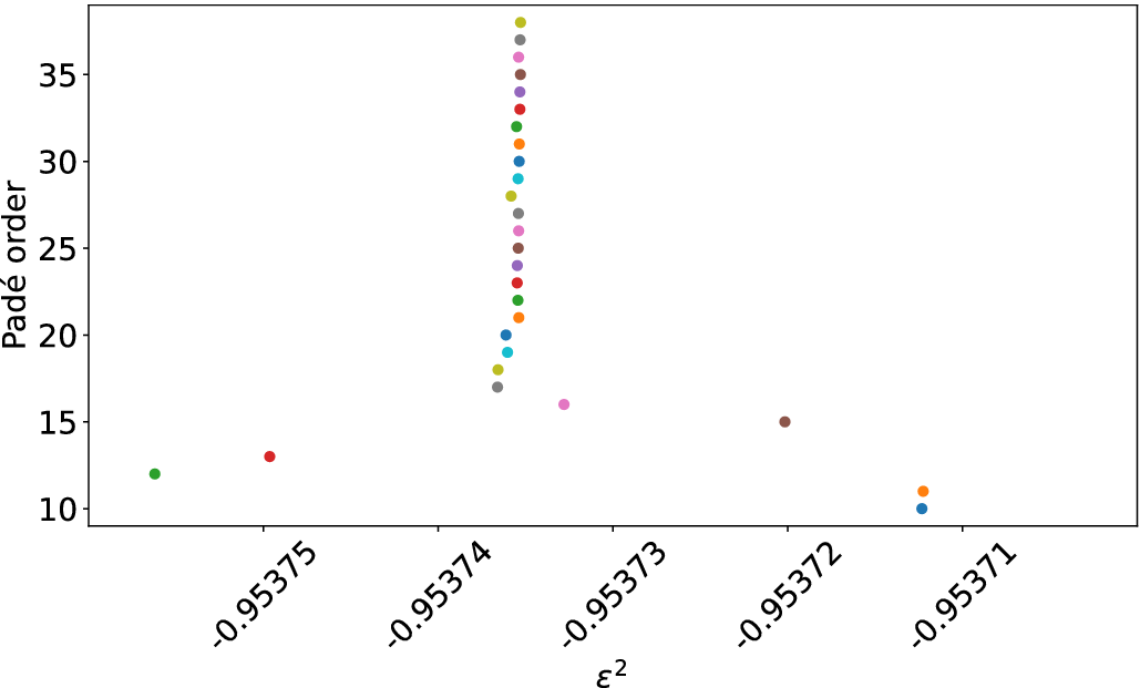
In addition to the visual inspection of the Domb–Sykes plot, and the use of Aitken extrapolation, a third check to locate the singularity is to investigate the zeros of the Padé approximants. We did this using the root-finding function for polynomials in the Python library numpy. We found that the denominator in each fraction has a zero near $-0.95$ . As the order of the approximants increases, these zeros converge to approximately $-0.953\,735\,3$ , shown in Figure 8. This agrees with the results of the Aitken extrapolation to five significant figures, providing strong support for this being the location of the singularity.

Figure 8

The Padé poles near $\epsilon ^2=-0.95$ , shown for Padé approximants from [10/10] to [38/38]. These converge near $-0.953\,735\,3$ .

Figure 8 Long description

The x-axis is labeled epsilon super 2 and ranges from negative 0.95375 to negative 0.95371. The y-axis is labeled Padé order and ranges from 10 to 35.

* At lower Padé orders (10 to 15), data points are scattered widely across the x-axis between negative 0.95375 and negative 0.95371.

* As the Padé order increases from 17 to 20, the points begin to cluster and move toward a central x-value.

* From Padé order 20 up to 38, the points form a nearly vertical line, converging tightly around an epsilon super 2 value of approximately negative 0.953735.

* The points are color-coded by order, showing a clear upward trend toward a singular vertical asymptote.

We now present a comparison with lubrication theory (LT). By converting the domain to $\epsilon /2(1+\cos (x))<y<1$ , we can compare directly with the results of Tavakol et al. [Reference Tavakol, Froehlicher, Holmes and Stone13]. To do so, we have converted our results from flux at constant pressure gradient to pressure drop for constant flux, via the relation $\Delta P_x/P_x=Q_0/Q_{\text {numerical}}$ . This relation holds in the Stokes flow linear regime, where the flux is linearly proportional to the pressure gradient. The new domain includes a zeroth-order term in the lower boundary, as well as the first-order term, so the expansion must now include all modes up to order n, not just those of the same parity. These changes mean that there are flux terms at all integer powers of $\epsilon $ , not just even powers.

With a significant amount of algebra, the bulk flux for this channel geometry was calculated by hand in a similar way to Section 2 out to order $\mathcal {O}(\epsilon ^2)$ , and found to be

$$ \begin{align*} Q=\frac{1}{6}- \frac{\epsilon}{4}+\frac{\epsilon^2}{4}\bigg(1-\frac{2-\sinh(2)}{4(1-\sinh^2 (1))}\bigg)+ \mathcal{O}(\epsilon^3)\end{align*} $$

The series was then expanded numerically to order $\epsilon ^{160}$ , and Padé approximants formed from the coefficients. The upper plot in Figure 9 shows the pressure drop as $\epsilon $ goes from 0 (straight wall) to 1 (channel pinched shut). The numerical solution is shown with stars. We see that the higher-order terms bring the perturbation expansion ever closer to the numerical solution, while the higher-order Padé approximants and the LT results are visually identical with the numerical solution.

Figure 9

Comparison of pressure drop with lubrication theory (LT) in a channel with lower wall at $y=\epsilon /2(1+\cos x)$ and upper wall at $y=1$ . The upper plot shows the numerical results (stars) with the perturbation expansion (light blue dashed lines) at order $\mathcal {O}(\epsilon ^1)$ to $\mathcal {O}(\epsilon ^{160})$ , the lubrication theory and its first and second corrections, and [20/20], [40/40], [60/60], [80/80] Padé approximants. In the lower plot, the residuals (difference with numerics) are shown. Kinks in the LT plots are due to points where the residual changes sign.

Figure 9 Long description

The image consists of two vertically stacked line graphs sharing a horizontal axis labeled Wall amplitude epsilon, ranging from 0.00 to 1.00. A legend to the right applies to both panels.

Top Panel: Normalised Pressure drop. The vertical axis is logarithmic, ranging from 10 super 0 to 10 super 4. Black stars represent Numerical data, showing an exponential increase as epsilon approaches 1.00. Light blue dashed lines represent perturbation expansions from order epsilon super 1 to epsilon super 160. Solid lines for L T sub 0 (black), L T sub 2 (blue), and L T sub 4 (red) follow the numerical trend closely until high epsilon values. Four shades of orange/red lines represent Pade [20/20], [40/40], [60/60], and [80/80] approximants, which maintain accuracy further into the high epsilon range.

Bottom Panel: Residual vs Numerics. The vertical axis is logarithmic, ranging from 10 super -10 to 10 super 2. This panel plots the difference between the models and the numerical results. The L T sub 0 (black), L T sub 2 (blue), and L T sub 4 (green) lines show higher residuals that increase with epsilon. The Pade approximant lines (shades of red) show significantly lower residuals, fluctuating near the 10 super -10 baseline before rising sharply as epsilon exceeds 0.75. Numerous light blue dashed lines fill the background, representing the residuals of the various perturbation orders.

The lower frame in Figure 9 shows the difference between the approximations and the numerical solution. The absolute value of this residual is plotted using a log scale. We see that the expansion is better for small $\epsilon $ , even at low order in $\epsilon $ , whereas the LT approximation is quite good even for high values of $\epsilon $ , and clearly improves as the correction terms are added. At the highest value of $\epsilon $ used in the numerical method (0.975), the perturbation expansion requires terms at order $\epsilon ^{80}$ to match the standard LT method, and at order $\epsilon ^{160}$ to match the first correction to LT, $\mathcal {O}(\delta ^2)$ , where $\delta $ is the maximum-width-to-half-wavelength aspect ratio, in this case $1/\pi $ . Note the difference to our earlier definition of aspect ratio, which was wavelength to mean width. The reason such high-order terms are required here is that the error decays only as $\epsilon ^n$ near the radius of convergence. However, the Padé approximants are again very effective in increasing the accuracy. The [20/20] approximant beats the LT approximation at $\epsilon =0.975$ , and the [40/40] matches the second correction to LT $\mathcal {O}(\delta ^4)$ . The [80/80] approximant is significantly more accurate than all other methods shown here.

Note that in this formulation we do not encounter an analytic singularity within the physical regime, as we did in Figure 5. Instead the ratio of the coefficients converges to 1, corresponding to the expected physical pinch-off of the channel, explaining the slow convergence of the perturbation series as $\epsilon $ approaches 1.

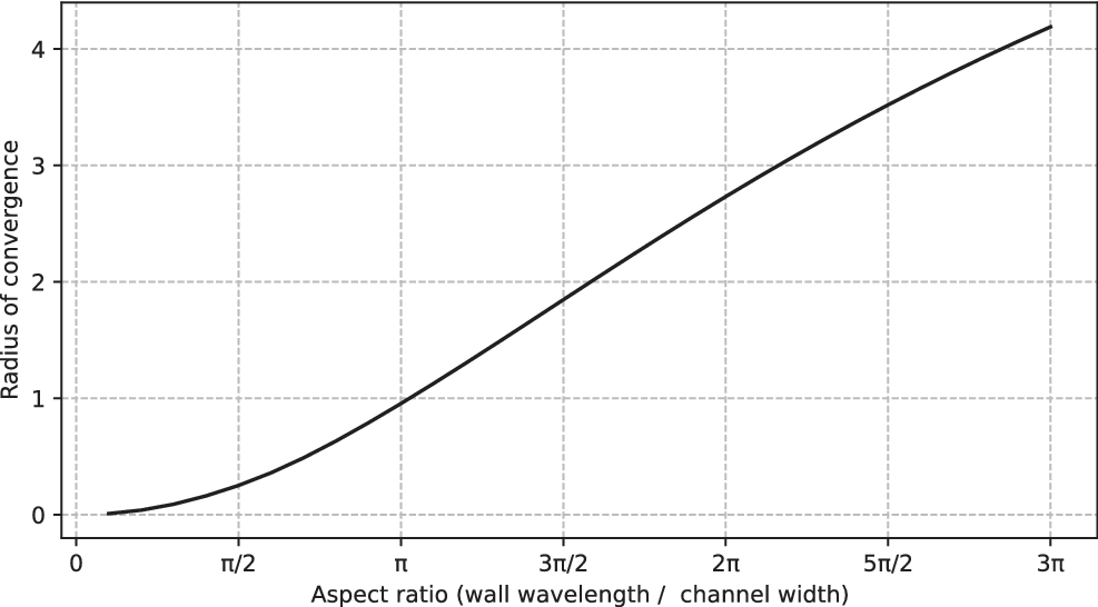
We conclude this section with an investigation into the effect of aspect ratio on the radius of convergence of the series. Reverting to our definition of aspect ratio as the wavelength divided by the mean channel width, the main study has been on a channel with aspect ratio $\pi $ . Keeping the mean channel width $-1<y<1$ , the wavelength has been varied as $-\alpha \pi <x<\alpha \pi $ and the lower wall is at $y=-1+\epsilon \cos (\alpha x)$ . Varying the value of $\alpha $ from 0.1 to 3, the radius of convergence was estimated from the asymptotic ratio of successive series coefficients, and then plotted in Figure 10. Note that once the radius of convergence is greater than 2, it is beyond the physical range, which should allow the series to converge for all physically meaningful values of the wall amplitude.

Figure 10

The effect of channel aspect ratio on radius of convergence of the series. The curve crosses the physically meaningful channel pinch-off point of $R=2$ near $1.6 \pi $ . For larger aspect ratios the series will converge for all physically sensible wall amplitudes.