2 Formulation of the problem

It will become clear that the theoretical framework to be developed in this study can be applicable for a quite wide range of MHD flows. However, it is advantageous to choose the flow configuration as simple as possible in order to concisely describe the main point of the theory and the computational methodology. The flow configuration we select for this purpose is plane Couette flow, a flow between two mutually moving parallel walls; see figure 1(a). Choosing the wall speed $U$ and the half-gap $h$ as the velocity and the length scales, respectively, the non-dimensional MHD equations can be written as

(2.1)$$\begin{eqnarray}\displaystyle & \displaystyle \frac{\text{D}\boldsymbol{u}}{\text{D}t}-(\boldsymbol{b}\boldsymbol{\cdot }\unicode[STIX]{x1D735})\boldsymbol{b}=-\unicode[STIX]{x1D735}p+\frac{1}{R}\unicode[STIX]{x1D6FB}^{2}\boldsymbol{u},\quad \unicode[STIX]{x1D735}\boldsymbol{\cdot }\boldsymbol{u}=0, & \displaystyle\end{eqnarray}$$

(2.2)$$\begin{eqnarray}\displaystyle & \displaystyle \frac{\text{D}\boldsymbol{b}}{\text{D}t}-(\boldsymbol{b}\boldsymbol{\cdot }\unicode[STIX]{x1D735})\boldsymbol{u}=\frac{1}{R_{m}}\unicode[STIX]{x1D6FB}^{2}\boldsymbol{b},\quad \unicode[STIX]{x1D735}\boldsymbol{\cdot }\boldsymbol{b}=0. & \displaystyle\end{eqnarray}$$

Here $\unicode[STIX]{x1D735}=(\unicode[STIX]{x2202}_{x},\unicode[STIX]{x2202}_{y},\unicode[STIX]{x2202}_{z})$ is the gradient in the Cartesian coordinates and $\text{D}/\text{D}t=\unicode[STIX]{x2202}_{t}+(\boldsymbol{u}\boldsymbol{\cdot }\unicode[STIX]{x1D735})$ is the material derivative. Note that for the magnetic field, the corresponding Alfvén wave speed is non-dimensionalised by the velocity scale. The first set of equations are the Navier–Stokes equations, which represent the conservation of momentum and mass, while the second set of equations are found from the Maxwell equations and Ohm’s law. Kinematic dynamo studies assume the smallness of the magnetic field $\boldsymbol{b}=(b_{x},b_{y},b_{z})$ so that the Lorentz force term $(\boldsymbol{b}\boldsymbol{\cdot }\unicode[STIX]{x1D735})\boldsymbol{b}$ is negligible in (2.1). In that case, the magnetic field is found from a linear analysis of (2.2), because the velocity $\boldsymbol{u}=(u_{x},u_{y},u_{z})$ and the pressure $p$ are determined from (2.1). As our interest here is the amplitude of the magnetic field, fully nonlinear analysis is necessary.

Figure 1.

(a) Configuration of dimensional plane Couette flow and its laminar solution. (b) The nonlinear steady plane Couette flow solution due to Nagata (Reference Nagata1990), Clever & Busse (Reference Clever and Busse1992). $R=236.4$. The box size is $[0,2\unicode[STIX]{x03C0}/\unicode[STIX]{x1D6FC}]\times [-1,1]\times [0,\unicode[STIX]{x03C0}]$, where $\unicode[STIX]{x1D6FC}=300/R\approx 1.27$. The solution is purely hydrodynamic, and corresponds to the green dot at $\unicode[STIX]{x1D716}=1.79\times 10^{-5}$ in figure 2. The streak structure is shown by the grey isosurface of zero streamwise velocity. The red and blue isosurfaces illustrate the streamwise vorticity by showing 70 % of the maximum and minimum values, respectively.

The magnetic and hydrodynamic Reynolds numbers are defined as $R_{m}=Uh/\unicode[STIX]{x1D702}$ and $R=Uh/\unicode[STIX]{x1D708}$, respectively, using the kinematic viscosity $\unicode[STIX]{x1D708}$ and Ohmic diffusivity $\unicode[STIX]{x1D702}$ of the fluid. The flow is assumed to be periodic in both $x\in [0,2\unicode[STIX]{x03C0}/\unicode[STIX]{x1D6FC}]$ and $z\in [0,\unicode[STIX]{x03C0}]$, with the streamwise wavenumber $\unicode[STIX]{x1D6FC}$. The box dimensions seen in figure 1(b) are close to those used in Hamilton et al. (Reference Hamilton, Kim and Waleffe1995), and as seen in that paper, typically only one streak is generated in the flow. The walls at $y=\pm 1$ are no-slip, and either perfectly conducting or insulating (Roberts Reference Roberts1964). Dynamos are self-excited MHD solutions, so any external magnetic effects must be switched off. We do not use the small-scale isotropic, non-helical external forcing term used in the majority of shear-driven dynamo studies (Yousef et al. Reference Yousef, Heinemann, Schekochihin, Kleeorin, Rogachevskii, Iskakov, Cowley and McWilliams2008a,Reference Yousef, Heinemann, Rincon, Schekochihin, Kleeorin, Rogachevskii, Cowley and McWilliamsb; Tobias & Cattaneo Reference Tobias and Cattaneo2013; Teed & Proctor Reference Teed and Proctor2017). Therefore, the only mechanism of energy input to the system is the shear due to the movement of the walls.

The system has the laminar Couette flow solution $\boldsymbol{u}=(y,0,0),\boldsymbol{b}=(0,0,0)$. There is no linear instability at all in this flow, unlike cylindrical (Willis & Barenghi Reference Willis and Barenghi2002) or spherical (Guervilly & Cardin Reference Guervilly and Cardin2010) Couette dynamo problems. The proof is simple. First, we note that Squire’s theorem is applicable even when magnetic effects are present, and thus it is sufficient to look for $z$-independent two-dimensional perturbation (Squire Reference Squire1933; Drazin & Reid Reference Drazin and Reid1981). Then from the Zel’dovich theorem (Zel’dovich Reference Zel’dovich1957), there is no exponentially growing magnetic perturbations. Finally, as shown by Romanov (Reference Romanov1973), there is no linear instability for purely hydrodynamic plane Couette flow.

Transition to turbulence nonetheless occurs by finite-amplitude perturbations (Nauman & Blackman Reference Nauman and Blackman2017). For the purely hydrodynamic case $\boldsymbol{b}\equiv \mathbf{0}$, the non-trivial steady solution found in Nagata (Reference Nagata1990) and Clever & Busse (Reference Clever and Busse1992) is responsible for this subcritical transition; here we reproduce the same solution in figure 1(b). The flow field of the solution is characterised by streaks – namely, inhomogeneity of the streamwise velocity swept by the streamwise vortices. A detailed description of the numerical code used can be found in Deguchi, Hall & Walton (Reference Deguchi, Hall and Walton2013) and Deguchi (Reference Deguchi2019b). The scheme first discretises (2.1) and (2.2) by means of the spectral method, and then Newton’s method is applied to find steady unstable solutions. To produce a reliable numerical result, up to 12 and 30 Fourier harmonics are taken in $x$ and $z$, respectively, while 70 Chebyshev modes are used in $y$.

3 Theoretical and numerical analyses

Figure 2.

Bifurcation diagram of the dynamo solution branches. Here $\unicode[STIX]{x1D6FC}_{0}\equiv \unicode[STIX]{x1D6FC}R_{m}=300$ and $P_{m}=1$. Red solid curve: perfectly conducting walls. Blue dashed curve: perfectly insulating walls. The green dot corresponds to the pitchfork bifurcation point where the red branch emanates from the kinematic dynamo action on top of the streaky field shown in figure 1(b). Panel ($a$) shows that both branches can be continued towards the infinite-Reynolds-number limit ($\unicode[STIX]{x1D716}=0$). The solutions for $\unicode[STIX]{x1D716}<0$ do not have any physical meaning; see (3.1).

The streak field for example seen in figure 1(b) is three-dimensional and hence can support a kinematic dynamo action, whose onset provides the bifurcation point of nonlinear dynamo solution branches. Throughout our computations the magnetic Prandtl number $P_{m}=R_{m}/R=\unicode[STIX]{x1D708}/\unicode[STIX]{x1D702}$ is fixed to be unity. Also the streamwise wavenumber is set to be $\unicode[STIX]{x1D6FC}=300/R$ for later convenience, unless otherwise specified. The bifurcation diagram shown in figure 2 can best illustrate the emergence of the dynamo solution branches. Here we measure the magnetic field amplitude by the maximum of $|\overline{B}_{x}|$, where $\overline{B}_{x}(y)$ is the streamwise magnetic field averaged in $x$ and $z$. The horizontal axis is

(3.1)$$\begin{eqnarray}\displaystyle \unicode[STIX]{x1D716}=R_{m}^{-2}. & & \displaystyle\end{eqnarray}$$

We shall shortly see that the introduction of this small parameter is the key to reaching our goals.

When the walls are perfectly conducting, the kinematic dynamo problem (2.2) possesses a real eigenvalue, which passes thorough zero at $R=236.4$; that is, the parameter used in figure 1(b). This solution corresponds to the green point at $\unicode[STIX]{x1D716}=1.79\times 10^{-5}$ in figure 2. The red curve is one of the dynamo solution branches produced by the pitchfork bifurcation at this point. The other dynamo solution branch exactly overlaps this curve because of the transformation $\boldsymbol{b}\rightarrow -\boldsymbol{b}$ mapping one solution to the other; equations (2.1) and (2.2) are invariant under this transformation because the magnetic field is a pseudo-vector in the MHD framework.

An alternative way to obtain a dynamo solution is by seeking nonlinear solutions to an externally magnetised system and then examining the limit of vanishing external magnetic field. This approach resulted in a successful strategy for perfectly insulating walls in the previous study (Deguchi Reference Deguchi2019a,Reference Deguchib); the corresponding dynamo solution branch is shown by the blue dashed curve in figure 2.

Having determined nonlinear dynamo solution branches, we will now continue them to the large-$R_{m}$ limit. Because of the choice $P_{m}=1$, this limit corresponds also to the large-$R$ limit. We begin the analysis by applying the long-wavelength rescaling

(3.2)$$\begin{eqnarray}\displaystyle x=R_{m}X & & \displaystyle\end{eqnarray}$$

with

(3.3)$$\begin{eqnarray}\displaystyle & \displaystyle (u_{x},u_{y},u_{z},p)=(U_{x},R_{m}^{-1}U_{y},R_{m}^{-1}U_{z},R_{m}^{-2}P), & \displaystyle\end{eqnarray}$$

(3.4)$$\begin{eqnarray}\displaystyle & \displaystyle (b_{x},b_{y},b_{z})=(B_{x},R_{m}^{-1}B_{y},R_{m}^{-1}B_{z}), & \displaystyle\end{eqnarray}$$

which makes the steady version of (2.1) and (2.2) take the form

(3.5)$$\begin{eqnarray}\displaystyle & \displaystyle (\boldsymbol{U}\boldsymbol{\cdot }\unicode[STIX]{x1D735})\boldsymbol{U}-(\boldsymbol{B}\boldsymbol{\cdot }\unicode[STIX]{x1D735})\boldsymbol{B}=-\unicode[STIX]{x1D735}_{\unicode[STIX]{x1D716}}P+P_{m}\triangle _{\unicode[STIX]{x1D716}}\boldsymbol{U},\quad \unicode[STIX]{x1D735}\boldsymbol{\cdot }\boldsymbol{U}=0, & \displaystyle\end{eqnarray}$$

(3.6)$$\begin{eqnarray}\displaystyle & \displaystyle (\boldsymbol{U}\boldsymbol{\cdot }\unicode[STIX]{x1D735})\boldsymbol{B}-(\boldsymbol{B}\boldsymbol{\cdot }\unicode[STIX]{x1D735})\boldsymbol{U}=\triangle _{\unicode[STIX]{x1D716}}\boldsymbol{B},\quad \unicode[STIX]{x1D735}\boldsymbol{\cdot }\boldsymbol{B}=0. & \displaystyle\end{eqnarray}$$

Here $\unicode[STIX]{x1D735}$ is redefined as $(\unicode[STIX]{x2202}_{X},\unicode[STIX]{x2202}_{y},\unicode[STIX]{x2202}_{z})$, and

(3.7a,b)$$\begin{eqnarray}\displaystyle \unicode[STIX]{x1D735}_{\unicode[STIX]{x1D716}}=(\unicode[STIX]{x1D716}\unicode[STIX]{x2202}_{X},\unicode[STIX]{x2202}_{y},\unicode[STIX]{x2202}_{z}),\quad \triangle _{\unicode[STIX]{x1D716}}=\unicode[STIX]{x1D716}\unicode[STIX]{x2202}_{X}^{2}+\unicode[STIX]{x2202}_{y}^{2}+\unicode[STIX]{x2202}_{z}^{2}. & & \displaystyle\end{eqnarray}$$

Note that no approximation has been made at this stage. In the rescaled coordinate, the flow is periodic in $[0,2\unicode[STIX]{x03C0}/\unicode[STIX]{x1D6FC}R_{m}]$, so we define the rescaled wavenumber $\unicode[STIX]{x1D6FC}_{0}=\unicode[STIX]{x1D6FC}R_{m}$, where $\unicode[STIX]{x1D6FC}_{0}=300$.

Figure 3.

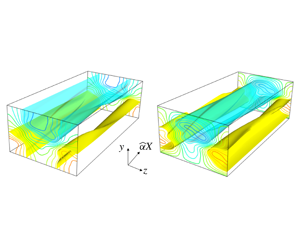
The streamwise magnetic field generated at infinite Reynolds number ($\unicode[STIX]{x1D716}=0$ in figure 2). $\unicode[STIX]{x1D6FC}_{0}\equiv \unicode[STIX]{x1D6FC}R_{m}=300$ and $P_{m}=1$. The box size is $[0,2\unicode[STIX]{x03C0}]\times [-1,1]\times [0,\unicode[STIX]{x03C0}]$. The yellow/blue surfaces are the isosurface of 50 % of the maximum/minimum, respectively. (a) Perfectly conducting walls. (b) Perfectly insulating walls.

The underlying motivation behind the scaling is somewhat similar to Prandtl’s boundary layer theory; more precisely, equations (3.5) and (3.6) at the limit $\unicode[STIX]{x1D716}\rightarrow 0$ are similar to the so-called ‘boundary region equations’, used in the boundary layer and microchannel flow studies (Kemp Reference Kemp1951; Fletcher Reference Fletcher1988; Hall Reference Hall1988; Rubin & Tannehill Reference Rubin and Tannehill1992; Deguchi et al. Reference Deguchi, Hall and Walton2013). With this scaling, some diffusive terms are still retained even at the large-Reynolds-number limit. This is because the driving mechanisms brought about by the shear are multiplied by the $x$ derivative, which is small from (3.2); hence the viscous–convective balance is always achieved. This diffusivity allows us to continue the solution branch across $\unicode[STIX]{x1D716}=0$, as shown in figure 2. In fact, the streamwise magnetic field shown in figure 3 suggests that the limiting flow field remains nicely smooth.

There is one minor technical remark that should be made here. If one uses the toroidal–poloidal potential decomposition for the flow field, some special care must be taken in the scaling of the potentials to avoid the singularity of the Jacobian matrix at $\unicode[STIX]{x1D716}=0$; see Deguchi et al. (Reference Deguchi, Hall and Walton2013). Alternatively, one can confirm that the initial guess created by a linear interpolation of nearby two solutions (at $\unicode[STIX]{x1D716}=10^{-12}$ and $-10^{-12}$, say) gives a very small residue with which the input data can be accepted as an accurate solution.

Figure 4.

The generated mean magnetic field for $\unicode[STIX]{x1D6FC}_{0}=300$. The solid curve is the limiting result (the same solutions as figure 3). The red points are the finite-Reynolds-number result at $R_{m}=R=3000$. (a) Perfectly conducting walls. (b) Perfectly insulating walls.

The streaky hydrodynamic flow structure is qualitatively unchanged from that shown in figure 1(b), while the examination of figure 3 indicates that the generated magnetic field also forms a streaklike structure. The dynamo solution inherits the two symmetries seen in the hydrodynamic plane Couette solution (Nagata Reference Nagata1990; Clever & Busse Reference Clever and Busse1992)

(3.8)$$\begin{eqnarray}\displaystyle [u_{x},u_{y},u_{z}](x,y,z) & = & \displaystyle [-u_{x},-u_{y},u_{z}](-x,-y,z+\unicode[STIX]{x03C0}/2)\nonumber\\ \displaystyle & = & \displaystyle [u_{x},u_{y},-u_{z}](x+\unicode[STIX]{x03C0}/\unicode[STIX]{x1D6FC},y,-z),\end{eqnarray}$$

with the same symmetries satisfied for the magnetic field. It is widely acknowledged in hydrodynamic studies that the latter shift–reflection symmetry is responsible for the sinusoidal meandering of the streak. The transformation (3.2) implies that, for large enough $R_{m}$, streamwise development of the flow is so slow that it may locally look almost two-dimensional. However, that streamwise modulation is nevertheless crucial in sustaining the dynamo mechanism because if it is absent there should be no dynamo solution from the parallel flow manifestation of Cowling’s antidynamo theorem (Cowling Reference Cowling1934).

The flow field quickly converges to the limiting result with increasing $R_{m}$. Figure 4 compares the mean magnetic field $\overline{B}_{x}$ of the limiting and finite-Reynolds-number solutions. Even at $R_{m}$ as low as order 10³, the two results are very close to each other. At higher $R_{m}$, of order 10⁴, the finite-Reynolds-number result is graphically indistinguishable from the limiting result.

Figure 5.

(a) The $\unicode[STIX]{x1D6FC}_{0}$ dependence of the limiting dynamo solutions ($\unicode[STIX]{x1D716}=0,P_{m}=1$). Red solid curve: perfectly conducting walls. Blue dashed curve: perfectly insulating walls. (b–d) Visualisation of the electric current strength $|\boldsymbol{j}|$ generated by the corresponding dynamo solutions indicated in (a). Grey transparent/green surface represents 50 %/60 % maximum value.

The reason for the rapid convergence can be explained by the formal asymptotic analysis. We first remark here that the large-Reynolds-number limit is a singular perturbation problem, where the ideal (diffusionless) problem may not produce the same result as the $R_{m}^{-1}\rightarrow 0$ limit of the diffusive problem. The diffusion effect is in fact not negligible when the flow develops a small-scale structure. This is the reason why the formal asymptotic analysis of high-Reynolds-number flows usually involves complicated matched asymptotic expansions.

Having said that, the rescaled system of (3.5)–(3.6) admits the regular asymptotic expansions

(3.9)$$\begin{eqnarray}\displaystyle & \displaystyle \boldsymbol{U}=\boldsymbol{U}_{0}(X,y,z)+\unicode[STIX]{x1D716}\boldsymbol{U}_{1}(X,y,z)+O(\unicode[STIX]{x1D716}^{2}), & \displaystyle\end{eqnarray}$$

(3.10)$$\begin{eqnarray}\displaystyle & \displaystyle \boldsymbol{B}=\boldsymbol{B}_{0}(X,y,z)+\unicode[STIX]{x1D716}\boldsymbol{B}_{1}(X,y,z)+O(\unicode[STIX]{x1D716}^{2}), & \displaystyle\end{eqnarray}$$

(3.11)$$\begin{eqnarray}\displaystyle & \displaystyle P=P_{0}(X,y,z)+\unicode[STIX]{x1D716}P_{1}(X,y,z)+O(\unicode[STIX]{x1D716}^{2}), & \displaystyle\end{eqnarray}$$

for small $\unicode[STIX]{x1D716}$. The crux of the argument is that, in our particular equilibrium invariant solutions, all the small-scale structures are screened out. As was mentioned in § 1, the solutions satisfy the MHD equations exactly within numerical accuracy, and hence, in this sense, there is no model reduction necessary to isolate large-scale coherent structures.

The leading-order solution $(\boldsymbol{U}_{0},\boldsymbol{B}_{0},P_{0})$ is what we found by letting $\unicode[STIX]{x1D716}\rightarrow 0$ in the rescaled system of (3.5)–(3.6). The correction to the leading-order part is of $O(\unicode[STIX]{x1D716})$, which is numerically very small even at moderately high $R_{m}$. Clearly, the scaling (3.4) and the asymptotic expansions (3.10) indicate that the streamwise magnetic field eventually becomes independent of $R_{m}$. Therefore, the generated magnetic field is, indeed, finite at the asymptotic limit.

The strength of the dynamo action gets stronger with decreasing $\unicode[STIX]{x1D6FC}_{0}$, as shown in figure 5(a). For large $\unicode[STIX]{x1D6FC}_{0}$, on the other hand, the dynamo becomes less effective; this observation is certainly consistent with Deguchi (Reference Deguchi2019a,Reference Deguchib), where theoretical and numerical evidence was given for the $O(\unicode[STIX]{x1D716}^{1/6})$ magnetic field generation at the shorter wavelength $\unicode[STIX]{x1D6FC}=O(1)$. Note also that in Deguchi (Reference Deguchi2019b) the asymptotic problem is solved with a regularisation effect whose strength is controlled by a parameter. On the other hand, the asymptotic problem obtained in this paper does not require such regularisation.

The electric current $\boldsymbol{j}=\unicode[STIX]{x1D735}\times \boldsymbol{b}$ produced by the dynamo mechanism is also $O(\unicode[STIX]{x1D716}^{0})$. In figure 5(b–d) we use the magnitude of it to see the $\unicode[STIX]{x1D6FC}_{0}$ dependence of the field structure of the dynamos. The green blobs enclosing the region where the strong current is generated are shortened in the streamwise direction for smaller $\unicode[STIX]{x1D6FC}_{0}$; compare figure 5(d) for $\unicode[STIX]{x1D6FC}_{0}=300$ and figure 5(c) for $\unicode[STIX]{x1D6FC}_{0}=200$. That streamwise concentration of the structure affects the decay of the streamwise Fourier coefficients, and hence the computation was double-checked using 18 streamwise Fourier modes. The convergence problem becomes even more serious on approaching the saddle-node point (b), because of the complicated field structure developed in all three directions. We are unable to determine if it is possible to round the saddle-node point. Note that, unlike finite-Reynolds-number computations, the solution branch of an asymptotically reduced problem may be terminated due to a mathematical singularity; see Dempsey et al. (Reference Dempsey, Deguchi, Hall and Walton2016) for example.

4 Summary and discussion

We have demonstrated that there are self-consistent, subcritical, nonlinear and three-dimensional dynamo solutions that persist at infinite hydrodynamic and magnetic Reynolds numbers. The homogeneous shear, which is used as an external base driving mechanism of the dynamos, presents as a large-scale background structure in many real-world problems (Ossendrijver Reference Ossendrijver2003; Monchaux et al. Reference Monchaux, Berhanu, Bourgoin, Moulin, Odier, Pinton, Volk, Fauve, Mordant and Pétrélis2007; Charbonneau Reference Charbonneau2014; Rincon Reference Rincon2019). Although such base flows may be stable with respect to small perturbations, finite-amplitude dynamos can be driven indirectly via the three-dimensional nonlinear mechanism. The key to the successful computation of the dynamos at the large-Reynolds-number limit is the method of invariant solutions, which allows us to isolate the large-scale structure without any ad hoc assumptions. The nonlinear dynamo solutions found are almost always unstable. As established in many previous purely hydrodynamic and magneto-hydrodynamic studies, at least for the transitional regime, such unstable solutions typically constitute a mathematically rational ‘backbone’ on which large-scale coherent structures in turbulence hang (Hamilton et al. Reference Hamilton, Kim and Waleffe1995; Waleffe Reference Waleffe1997; Hof et al. Reference Hof, van Doorne, Westerweel, Nieuwstadt, Faisst, Eckhardt, Wedin, Kerswell and Waleffe2004; Rincon et al. Reference Rincon, Ogilvie and Proctor2007; Gibson et al. Reference Gibson, Halcrow and Cvitanovic2008; Herault et al. Reference Herault, Rincon, Cossu, Lesur, Ogilvie and Longaretti2011; Kawahara et al. Reference Kawahara, Uhlmann and van Veen2012; Riols et al. Reference Riols, Rincon, Cossu, Lesur, Longaretti, Ogilvie and Herault2013; Willis et al. Reference Willis, Cvitanovic and Avila2013).

The finite-amplitude dynamo magnetic field generation at the large-$R_{m}$ limit has been conclusively determined for the first time, within a framework that is fully consistent to the asymptotic behaviour of the finite-$R_{m}$ results. The rapid convergence of the finite-Reynolds-number results towards the limiting result is justified by the asymptotic analysis. The numerical limiting process has been proved successful for the two popularly used magnetic boundary conditions on the walls. Thus we expect that the effective streaky magnetic field generation mechanism is robust against the flow configuration, so that a similar structure may also appear in various MHD flows.

There are some astrophysical flows where the present method could be applicable, but with some extensions. Threadlike structures reminiscent of the streak can for example be found in the observation of the Sun’s atmosphere (Okamoto et al. Reference Okamoto, Antolin, De Pontieu, Uitenbroek, van Doorsselaere and Yokoyama2015). For such atmospheric flows the effects of compressibility and stratification must be included to find quantitative features of the dynamos. Streaklike subcritical dynamos have also been observed in shear flows under Kepler rotation, and believed to play an important role in angular momentum transport of accretion disks (Rincon et al. Reference Rincon, Ogilvie and Proctor2007; Herault et al. Reference Herault, Rincon, Cossu, Lesur, Ogilvie and Longaretti2011; Riols et al. Reference Riols, Rincon, Cossu, Lesur, Longaretti, Ogilvie and Herault2013). At least it was numerically confirmed for moderate $R_{m}$ that the shear-driven dynamo obtained in Yousef et al. (Reference Yousef, Heinemann, Schekochihin, Kleeorin, Rogachevskii, Iskakov, Cowley and McWilliams2008a) works even for the rotating case (Yousef et al. Reference Yousef, Heinemann, Rincon, Schekochihin, Kleeorin, Rogachevskii, Cowley and McWilliams2008b). More recently, the existence of similar subcritical dynamos in global cylindrical coordinate simulations has been reported by Guseva et al. (Reference Guseva, Hollerbach, Willis and Avila2017). In cylindrical geometry, there is a maximal length scale in the streamwise (azimuthal) direction. This means that the cross-streamwise scale of the coherent structures must be small in order to apply the scaling of the dynamos discussed in this paper.

The present study focused only on $P_{m}=1$. The question therefore naturally arises as to how the magnetic field generation changes as that parameter varies. Within the asymptotic framework, $P_{m}$ is formally an $O(\unicode[STIX]{x1D716}^{0})$ quantity. Thus the range of $P_{m}$ within which the large-$R_{m}$ dynamos exist must be studied numerically in the future. The value of $P_{m}$ in plasma flows changes depending on the temperature and density; for example, the recent plasma experiment used noble gases to control $P_{m}$ within the range 0.2–12 (Collins et al. Reference Collins, Clark, Cooper, Flanagan, Khalzov, Nornberg, Seidlitz, Wallace and Forest2014). The tentative calculations suggest that certainly our limiting dynamo solutions exist for the relevant range of $P_{m}$. This result may motivate experimentalists to use a plasma flow as simple as that through a long straight pipe to generate a strong streaky magnetic field. Such experiments may help answering the question whether the invariant solutions remain relevant to turbulent dynamics at large $R_{m}$ and $R$, beyond the transitional regime.