


Introduction
One possible impact of human activity on the global climate system is change in the surface mass balance of the polar ice sheets, resulting in a change in the global sea level. We need to be able to give accurate estimates of the future surface mass balance of Antarctica because it is the largest ice sheet on Earth. In response to a warmer climate, the Antarctic ice sheet appears more likely to thicken than to thin (Reference Ohmura and WildOhmura and Wild, 1995). This may be because warmer air can transport more moisture to the continent, whereas the temperature is unlikely to rise enough to increase significantly ice melting and runoff, although changes in cyclone frequency, strength and position might be expected that may complicate the picture. The modified surface mass balance of Antarctica may thus partially offset a sea-level rise from the melting of temperate and other polar glaciers (including Greenland) and the thermal expansion of the oceans. However, uncertainties remain (Reference Houghton, Jenkins and EphraumsHoughton and others, 1995).
Atmospheric general circulation models (GCMs) can be used to predict the future surface mass balance of the polar ice sheets. In order for these predictions to be reliable, it is first necessary to be sure that the GCM produces a reasonable simulation of the current surface mass balance. Much progress has been made in recent years in this respect (e.g. Reference Tzeng, Bromwich and ParishTzeng and others, 1994), due in part to increased horizontal resolution as a consequence of increased computing power (Reference Genthon, Jouzel, Déqué, Desbois and DésalmandGenthon and others, 1994). However, even if a model produces a good estimate of the current surface mass balance, it need not necessarily be for the correct reasons. For example, Reference Connolley and KingConnolley and King (1996) report that in the United Kingdom Meteorological Office (UKMO) GCM, which produces a good estimate of the Antarctic surface mass balance, only 30% of the water vapor precipitated over a large sector of East Antarctica is advected by explicit transport at the resolved scales. The rest is carried onto the continent through horizontal diffusion, which is a numerical convenience introduced to prevent small-scale instabilities and which can be seen as a parameterization of sub-gridscale atmospheric dynamics. Reference Connolley and KingConnolley and King (1996) conclude that it is doubtful whether a predicted surface mass balance for future climates is credible.
In this study, we used the Laboratoire de Météorologie Dynamique (LMD) stretched-grid GCM (provisionally called LMDz, where ’z’ stands for ’zoom’) with a horizontal resolution of about 100km over a large part of Antarctica. This is quite a high resolution, the grid spacing of most GCMs usually being only about 300–400 km. This high resolution is achieved by locally refining the grid over the region of interest at the expense of the rest of the globe. The model is global, so the interaction between the high-resolution region and the rest of the globe is treated consistently but computational cost is reasonable compared to a model with equal grid spacing everywhere.
We compare the spatial pattern of the simulated surface mass balance (in water equivalent (w.e.) a−1) to the observations, and, in order to evaluate the credibility or the simulation, we examine the annual cycle of the modeled precipitation over the whole continent and over the high plateau of East Antarctica. Furthermore, the high frequency variability of the simulated precipitation in Antarctica is addressed, and a typical synoptic situation leading to significant snowfall is briefly discussed.
The Model
The model is a new version of the LMD gridpoint GCM. The physical parameterizations are essentially those of the LMD-GCM Cycle 5 (Reference PolcherPolcher and others, 1991; Reference Harzallah and SadournyHarzallah and Sadourny, 1995). The most important differences between the LMD-GCM Ciyele 5 and the GCM used in this study is the ability to stretch the grid horizontally, and the different parameterization of the horizontal diffusion of small-scale waves that may be subject to future improvement. There is no horizontal diffusion of water vapor in the model, so all moisture transport is by the resolved winds. Thus, the problem identified by Reference Connolley and KingConnolley and King (1996) in the UKMO GCM does not affect this model. Some of the parameterizations are further adapted for polar climate and high resolution, and are described by Reference Krinner, Genthon, Li and Le VanKrinner and others (1997).
The primitive equations are integrated on a grid of 64 equally spaced points in longitude and 72 points in latitude, which are concentrated over Antarctica. This yields a meridional resolution of about 100 km over Antarctica, and approximately 700 km at the North Pole. Due to the convergence of the meridians towards the poles, the zonal resolution becomes high in the polar regions even with a low number of gridpoints in longitude. Figure 1 shows the effective zonal and meridional resolution as a function of latitude. Note that, although the nominal zonal resolution becomes infinite at the Pole because the meridians converge, the effective zonal model resolution does not, because of the action of a numerical zonal wave filler close to the pole. This filtering is necessary because an infinitely fine grid requires a vanishing integration time-step as a consequence of the Courant-Friedrich-Levy stability criterion. The zonal filter thus limits the effective zonal resolution to about 100 km polewards of 82°S.
The model resolution in km as a function of latitude, (a) meridional resolution, (b) zonal resolution.

The simulation presented here covers the five years from September 1986 to August 1991. The model was spun-up for three months from a synoptic snapshot. AMIP (Atmospheric Model Intercomparison Project) (Reference GatesGates, 1992) boundary conditions for the sea-surface temperatures were used. Sea-ice fraction was obtained from SSM/I satellite data (NSIDC, 1992). This is the same simulation as that presented in Reference Krinner, Genthon, Li and Le VanKrinner and others (1997).
Results
The annual mean surface mass balance
Figure 2 shows the annual mean surface mass balance as simulated by the model, as well as observations by Reference Giovinetto and BentleyGiovinetto and Bentley (1985). The model captures well the shape and the extent of the large area with low accumulation below 5 cm a−1, although this region extends too far towards the Coast on the Lambert Glacier and the eastern edge of the Ross Ice Shelf. Low accumulation on the ice shelves is a feature both of the model and the observations. However, the model underestimates the mass balance in these areas. Due to the relatively high horizontal resolution, the strong accumulation gradient near the coast is well captured in the simulations, and the model even succeeds in reproducing the higher accumulation values at the foot of the Transantarctic Mountains on the Ross Ice Shelf.
The annual mean surface mass balance in cm a−1 w.e., (a) as simulated by the model, (b) after Reference Giovinetto and BentleyGiovinetto and Bentley (1985), interpolated onto the model grid.
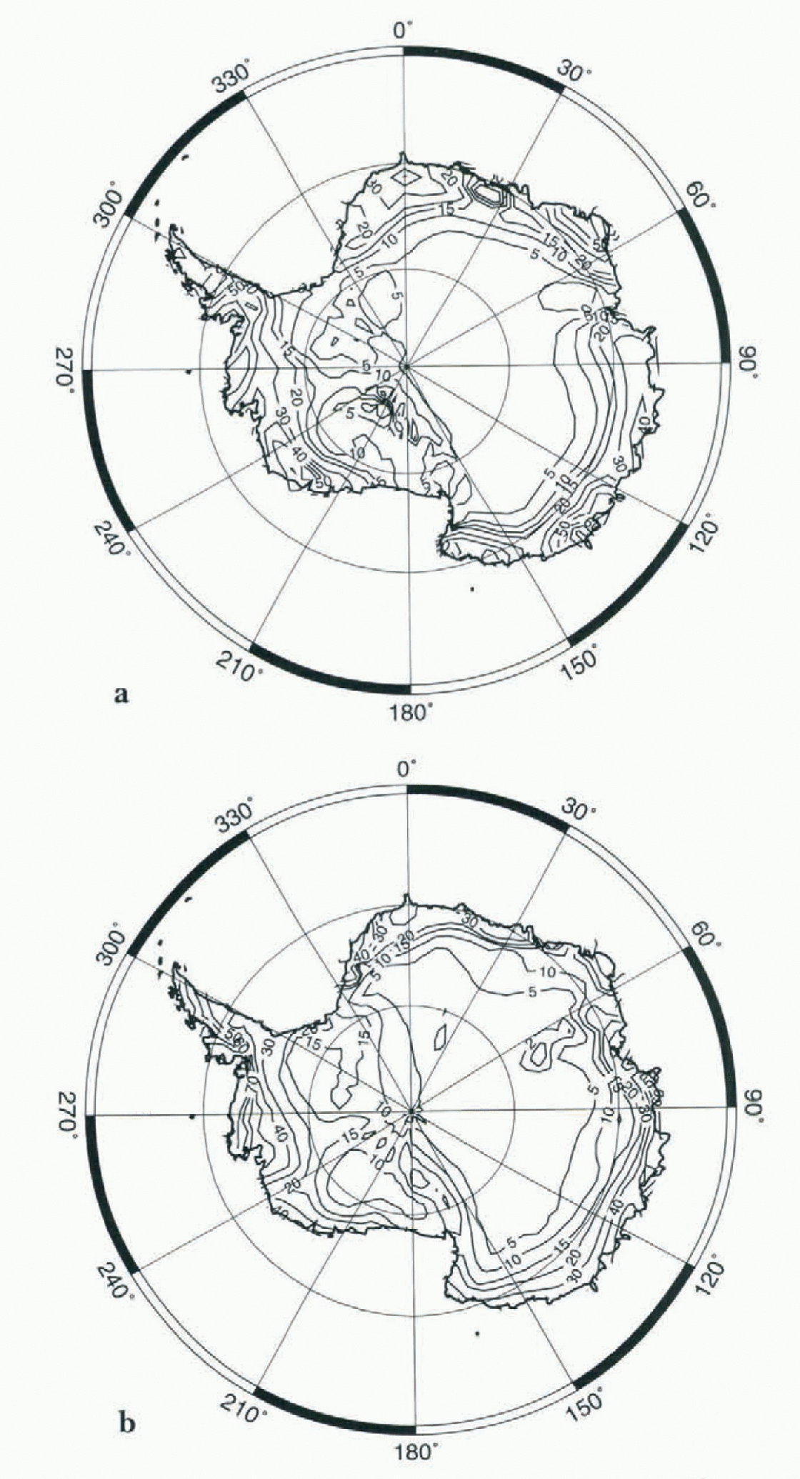
The zonal accumulation gradient over the Antarctic Peninsula is not sufficiently strong in the model. Because the Peninsula is relatively far north, the zonal resolution is only about 250 km. This means that the mountain ranges in this area are not resolved, leading to an underestimation of the orographic forcing of precipitation. However, the average accumulation over the Antarctic Peninsula is accurately reproduced.
As a whole, the general pattern of the surface mass balance is well simulated by the model. Including the ice shelves, the overall continental mean surface mass balance for the five years is 16.2 cm w.e. a−1 with the values for the individual years ranging from 16.0 to 16.4cm without any visible trend over the five years of the simulation. The value of 16.2 cm a−1 can thus be regarded as representative of the model climate. This compares favorably with the most recent estimations of the surface mass balance e.g. 15.4 cm a−1 by Reference Frolich and MorrisFrolich (1992) for the whole ice sheet). This estimation is based on the value of 14.3 cm a−1 given by Reference Giovinetto and BentleyGiovinetto and Bentley (1985) for the Antarctic excluding the Antarctica Peninsula. The uncertainty of these values is about 10%.
The annual cycle of the surface mass balance
Figure 3 displays the five-year mean monthly surface mass balance for the whole continent (Fig. 3a), and for the grid-points above 3000 m altitude, which thus belong to the East Antarctic plateau (Fig. 3b). In both cases, there is a clear minimum in summer, perhaps earlier on the Antarctic plateau than on the rest of the continent. For the continent as a whole, the snowfall maximum typically occurs in April or May with a broad maximum from February to October. In fact, developing the monthly time series of precipitation over the five years (Fig. 4a) shows there is often a secondary maximum between July and September, which is not visible in the five-year mean time series (Fig. 3a), because its timing is variable.
(a) Simulated monthly mean surface mass balance in mm month−1 fox the whole Antartic ice sheet. (b) Simulated monthly mean surface mass balance in mm month−1 for the gridpoints above 3000m. The diamonds show precipitation observations for the Vostok station from Reference Dolgin and PetrovaDolgin and Petrova (1977). The error bars denote the standard deviation between the individual five years of the simulation.

The monthly mean values of the accumulation for the individual 60 months of the five-year simulation in mm month−1. The time series begins in September 1986 and ends in August 1991, (a) for the whole of Antarctica, (b) for the gridpoints above 3000 m.
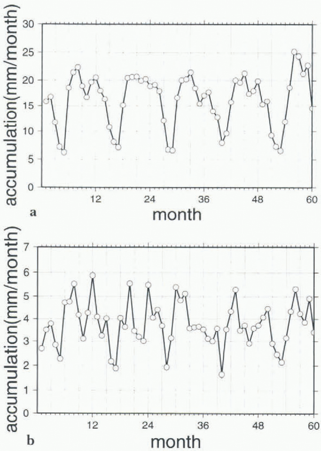
Above 3000m, when developing the same five-year monthly time series (Fig. 4b), there is strong semi-annual variation visible for most of the years, but again the timing of the individual peaks is variable, so that in the five-year mean time series (Fig. 3b), this signal becomes almost insignificant and only the annual cycle with a broad maximum in winter and a relatively sharp minimum in summer may be regarded as significant.
The monthly mean accumulation can be compared to precipitation observations from various Antarctic stations published by Reference Dolgin and PetrovaDolgin and Petrov (1977) and discussed by Reference BromwichBromwich (1988). For the high interior stations (Vostok and South Pole), the annual cycle seems to be reasonably simulated by the model, except that the maximum is probably a little early in the model and the summer minimum is too sharp. There is no sign of semi-annual variation in the observations.
However, the observations in central Antarctica, where the precipitation rates are low, are subject to significant uncertainty (Reference BromwichBromwich, 1988). The observed values from the East Antarctic coastal stations show the same seasonal trend, and Bromwich concludes that this kind of cycle — a maximum in winter and a minimum in summer – probably characterizes the entire East Antarctic ice sheet. However, Reference Budd, Reid and MintyBudd and others (1995), using the net atmospheric moisture convergence from the Gamma-Ray Astronomy at the South Pole (GASP) analyses, derived an annual cycle of the surface mass balance for the highest parts of Antarctica (above 2500m) with little systematic variation during the year, and maybe with a slight maximum in summer. On the other hand, as in this study, they found relatively high variability from year-to-year, and frequently the highest accumulation occurred around the equinoxes.
For the whole Antarctic ice sheet, the simulated annual cycle of the accumulation rate compares favorably to the annual cycle from the GASP (Reference Budd, Reid and MintyBudd and others, 1995) and the National Meteorological Center (NMC) (Reference YamazakiYamazaki, 1992) analyses, although it should be noted that the NMC analyses show a stronger semi-annual cycle than either the LMDz model or the GASP analyses. Note however that the NMC analyses were shown to be severely deficient in some respects (Reference Bromwich, Robasky, Cullather and vanWoertBromwich and others, 1995). Moreover, European Centre for Medium Range Weather Forecasting (ECMWF) analyses (Reference Bromwich, Robasky, Cullather and vanWoertBromwich and others, 1995) suggest a peak in July, and a broad maximum from April to September, which is again similar to the cycle simulated by LMDz.
Cyclonic activity in the Southern Ocean may be of considerable importance to precipitation occurrence in Antarctica. The continent is surrounded by a low pressure belt, which is commonly called the circumpolar trough (CPT). The depth and position of the CPT are linked to the strong latitudinal insolation gradients (Reference Loonvan Loon, 1967). In the LMDz GCM, as in many other GCMs (Reference Tzeng, Bromwich and ParishTzeng and others, 1993), the latitude of the CPT is generally underestimated bv several degrees (Reference Krinner, Genthon, Li and Le VanKrinner and others, 1997) compared to observations (Reference Xu, von Storch and van LoonXu and others, 1990). But these observations are drawn from various sources prior to 1981, so that, when comparing them to the LMDz simulations, one has to bear in mind that the differing time periods may be at least partly responsible for the differences. Note that the simulated latitude of the CPT compares well with the ECMWF analyses from 1985–91 (Reference Krinner, Genthon, Li and Le VanKrinner and others, 1997). The mean intensity of the CPT is also simulated well by the LMDz GCM, although it fails to reproduce the observed intensity of the semi-annual cycle. Note, however, that these cycles are subject to great inter-annual variability in the model, so that the details of the cycles may not be statistically robust (Reference Krinner, Genthon, Li and Le VanKrinner and others, 1997).
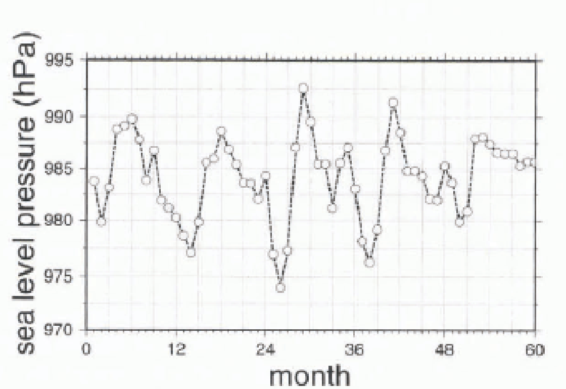
Figure 5 shows the five-year time series of the simulated depth of the CPT. There is a clear correlation between this time series and the five-year time series for the accumulation over the whole of Antarctica (Fig. 4a), although this correlation does not hold for all details (i.e. there are differences in the relative amplitudes of the minima and maxima). This is due to influences from other pertinent variables such as the latitudinal position of the CPT and the sea-ice extent.
The monthly mean values of the surface pressure of the CPT for the individual 60 months of the five-year simulation in hPa.
The accumulation over the Antarctic plateau above 3000 m seems to be more strongly influenced by the latitudinal position of the CPT (not shown), although the correlation is not clear since both signals are complicated and, again, other influences such as sea-ice extent and the intensity of the trough are important.
The short-term variability of precipitation
Figure 6a displays the 1990 time series of the simulated daily precipitation at the gridpoint that contains Dome C (123.0°E, 74.5°S, 3280m a.s.l.) in East Antarctica. The frequency of precipitation events is greatest during spring and autumn, and least in winter and summer. This is consistent with the Iivoycar time series of the monthly accumulation ahove 3000m presented in Figure 4b .
Daily values for 1990 for the gridbox representing Dome C. The LMDz model has a 360-day year, (a) precipitation in mm d−1. (b) surface pressure in hPa, (c) surface temperature in °C.
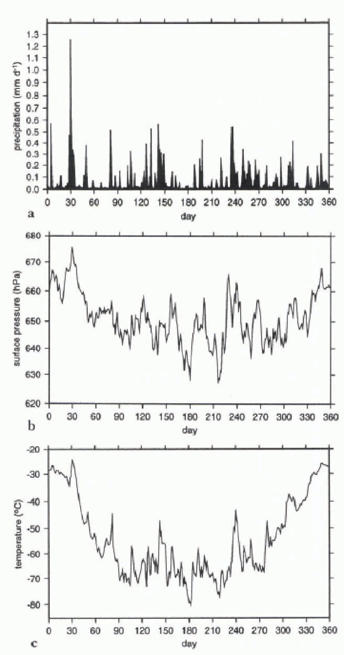
The model simulates very lew days with no solid precipitation. (Hereafter, “snowfall” will be used in the sense of “solid precipitation” that comprises precipitation of snow and ice crystals.) Rather, there is invariably at least a light snowfall background of about 0.005 mm d−1 (about 0.2 cm a−1), which thus accounts for about 5% of the annual accumulation. This background precipitation might correspond to the light ice-crystal precipitation often reported, even from clear skies that occurs during most of the year in the higher parts of Antarctica (Reference SchwerdtfegerSchwerdtfeger, 1984; Reference BromwichBromwich, 1988). Of course, clouds are diagnosed in the model when precipitation is simulated, but because of the very low temperatures these clouds can be optically so thin that the process can be identified as “clear sky” precipitation.
Even though mean precipitation has a definite minimum in summer (see the section entitled: The annual cycle of the surface mass balance), the largest single snowfall events occurs on day 30 of the year. Warmer air can contain more moisture, so that summer precipitation events, although rarer than in winter, can deposit a comparatively large quantity of water and contribute significantly to the annual surface mass balance. It is interesting to note that, during another simulated year, a similarly important single summer precipitation event was also simulated.
Both events are characterized by particular synoptic situation: a strong cyclone off the coast downslope of Dome C, and a relatively high-pressure area to the east of it (Fig. 7). The two systems together advect warm and moist air into the interior where precipitation then occurs. This air mass can even be traced to Vostok, where relatively high snow fall is simulated one day later than at Dome C. The synoptic situation discussed above is similar to the situation leading to intrusions of warm moist air into Antarctica and to subsequent precipitation in the interior as discussed by Reference BromwichBromwich (1988).
The simulated sea-level pressure (in hPa) on day 30 of 1990 minus the mean sea-level pressure for December, January and February for 1989 and 1990. Areas below-20 hPa are black, areas above +20 hPa are grey. Note the strong pressure gradient off the coast facing Dome C. The simulated sea-level pressure (in hPa) on day 30 of 1990 minus the mean sea-level pressure for December, January and February for 1989 and 1990. Areas below-20 hPa are black, areas above +20 hPa are grey. Note the strong pressure gradient off the coast facing Dome C. The simulated sea-level pressure (in hPa) on day 30 of 1990 minus the mean sea-level pressure for December, January and February for 1989 and 1990. Areas below-20 hPa are black, areas above +20 hPa are grey. Note the strong pressure gradient off the coast facing Dome C.
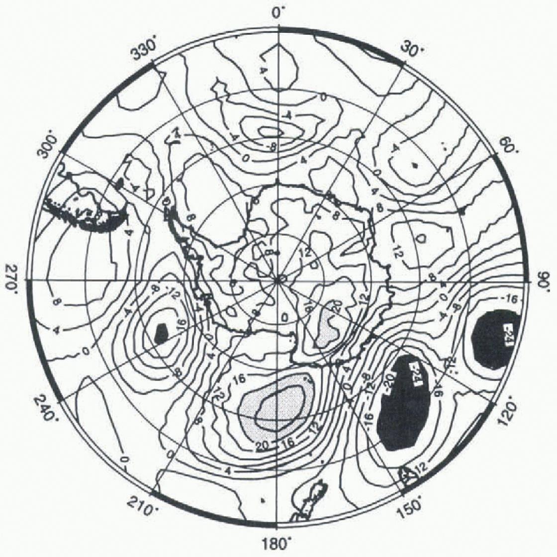
In most of the cases of high precipitation in the interior, a similar dipole situation off the coast can be observed. Note however that the low pressure does not intrude into the interior of Antarctica, although its anticyclonic counterpart to the east could help “push” it toward the interior. This is realistic, as it is well known that cyclones rarely penetrate into East Antarctica because of the blocking effect of the ice sheet (Reference MechosoMechoso, 1980).
In fact, the surface pressure at Dome C is particularly high and falling during the event, attaining its maximum one day before the precipitation (Fig. 6b). This is in agreement with the discussion by Reference BromwichBromwich (1988). At least in summer, precipitation in the interior occurs more often in association with high than with low surface pressure, although the correlation is not strong. In winter, there are sometimes snowfall episodes when the surface pressure over the whole interior of Antarctica drops by more than 10 hPa in one or two days, but that this is due to the intrusion of a cyclone is doubtful. On the other hand, and not surprisingly, there is a clear correlation between precipitation and temperature (Fig. 6c), pointing to the oceanic origin of the air masses that bring moisture into the continent. Note that Figures 6a and 6c reflect the increased cyclonic activity in winter and the relatively calm weather in summer.
Summary and Conclusions
The LMD stretched-grid GCM with a local horizontal resolution of 100km produces an accurate simulation of the surface mass balance of the Antarctic ice sheet, although the shell areas are too dry in the model and, due to a relatively low zonal resolution over the Antarctic Peninsula, the strong zonal variations of the mass balance in this region are not well captured. The model reproduces a maximum snow accumulation at the foot of the Transantarctic Mountains, but it underestimates the mass balance over the Amery Ice Shelf at the tongue of the Lambert Glacier. The total continental surface mass balance is 16.2 cm a−1, which compares favorably with estimates for the actual balance.
The seasonal cycle of precipitation shows a clear minimum in summer and a large maximum in winter, which is in keeping with observations. There is a large inter-annual variability of the secondary features of the annual cycle, but in most of the five years of the simulation, a semi-annual variation of the accumulation is visible. This may be linked to the semi-annual variation of the intensity of the circumpolar trough.
The short-term variability of snowfall in the model shows the clear influence of the cyclones off the East Antarctic coast, although, at least in summer, there is no sign of intrusion of these cyclones into the interior of the continent. Precipitation rarely drops to zero in the model. Rather, an almost permanent background snowfall accounts for about 5% of the total annual mean precipitation. This light, steady precipitation might be related to the occurrence of ice crystals in the lower atmosphere even during cloudless days.
Overall, the model produces a realistic simulation of the present-day precipitation in Antarctica. Further experiments with the model are planned, including an assessment of the dynamic aspects of cyclones. However, we are sufficiently confident to contemplate its use for the estimation of Antartic mass balance in other climates (e.g. ice ages and CO2 doubling experiments).
Acknowledgements
This research was supported by the Commission of the European Communities, Directorate General XII, under contract ENV4-CT95-0124 (Climate and Sea Level Change), and by the French Programme National d’Étude de la Dynamique du Climat. Computer time on a Cray C90 was provided by the Institut du Développement et des Ressources en Informatique Scientifique (CNRS) and by the Centre Grenoblois de Calcul Vectoriel (CEA). We are grateful to the Laboratoire de Météorologie Dynamique (ENS/CNRS) for providing the LMDz GCM, and P. Le Van and L. Li for their help. Comments and suggestions by D. Bromwich and two anonymous reviewers helped improve this work.



